Enhancing Sustainability in Watershed Management: Spatiotemporal Assessment of Baseflow Alpha Factor in SWAT

Abstract

The increasing frequency of extreme rainfall events poses significant challenges to sustainable water resource management, leading to severe natural disasters. To mitigate these challenges, understanding the hydrological characteristics of watersheds, especially baseflow, is critical for enhancing watershed resilience and supporting sustainable water quality and resource management. However, conventional watershed models often neglect the accurate simulation of baseflow recession. This study proposes a method for calculating and applying the alpha factor for each hydrologic response unit (HRU) in the Soil and Water Assessment Tool (SWAT), considering both temporal and spatial variability in baseflow. The study watershed has undergone significant development, increasing the need for effective water management strategies that promote long-term sustainability. The alpha factor was computed using BFlow2021, and its effectiveness was evaluated by comparing recession and baseflow estimates under different methods. The results indicate that incorporating monthly HRU-specific alpha factors significantly improves model predictions of recession characteristics, highlighting the need for a more spatially and temporally detailed approach in hydrological modeling. The proposed methodology can help clarify the connection between recession and baseflow and can be applied to ungauged stations, offering a valuable tool for sustainable watershed and water quality management.

1. Introduction

The occurrence of torrential rainfall caused by abnormal climate conditions and the disparity in regional rainfall distribution lead to severe natural disasters such as floods and droughts [1,2,3]. These phenomena threaten the water cycle system. Moreover, climate change and urbanization have increased the variability of runoff, decreased groundwater levels, and reduced baseflow, causing distortions in the water cycle [4]. Understanding the hydrological conditions of the watershed is important in addressing these issues. Various watershed modeling tools such as SWAT, Hydrological Simulation Program-FORTRAN (HSPF), and Storm Water Management Model (SWMM) are widely used for watershed management, both domestically and internationally [5,6,7,8,9]. However, existing watershed modeling studies present evaluation results using criteria that are very sensitive to greater values among observed and simulated data compared to low flow [10,11]. This means that inaccuracies in low flow regimes are often overlooked. It fails to accurately consider the characteristics of each hydrological component, with baseflow and low flows receiving relatively less attention than high flows and floods [12,13]. Therefore, there is a need to analyze and respond to baseflow, which significantly contributes to streamflow, accounting for over 40% of the annual average in many watersheds in South Korea [14].

Moreover, since baseflow delivers considerable loads of pollutants to the stream, in-depth research on baseflow and its associated pollutant loads is essential for sustainable water quality management in rivers [15,16]. Thus, baseflow estimation is a crucial component in water cycle analysis, contributing to both quantity and quality, and its variations and quantities over time must be assessed with proper goals [17,18]. For accessibility and convenience in estimating baseflow, various software programs like RECESS [19], RORA [20], BFlow [21], HYSEP [22], and WHAT [23] have been developed and used for various baseflow studies. Moreover, among watershed models, the SWAT has been widely assessed for its applicability across various watersheds, with various studies focusing on baseflow analysis [24,25]. Arnold and Allen [21] proposed calculating the alpha factor related to the recession by using long-term streamflow data in BFlow and then applying it to the SWAT groundwater module. Lee et al. [26] and Lee et al. [27] demonstrated the effectiveness of applying the alpha factor in SWAT, showing more accurate baseflow simulation results when SWAT was calibrated for recession periods using this factor. Moreover, Lee [28] proposed a methodology to apply a monthly alpha factor in SWAT to account for seasonal effects on baseflow regimes and demonstrated its validity. However, regarding the temporal variation of the alpha factor and its impact on streamflow and baseflow simulation in SWAT, the influence of spatial environmental heterogeneity within subbasins on the alpha factor and recession simulation also needs to be evaluated. Although SWAT is already designed to assign specific values for each hydrologic response unit (HRU), a method to calculate alpha factor values for each HRU considering spatial variations has not yet been developed. In other words, previous studies evaluated baseflow by applying a specific alpha factor to each HRU without considering temporal and spatial variations. Therefore, a study that applies the alpha factor in SWAT while considering both spatial and temporal variations is necessary to enhance the understanding of its impact on recession and baseflow. The objectives of this research are to suggest a strategy for assigning monthly alpha factors to each HRU, taking into account the spatial and temporal variations in recession characteristics, and to evaluate the effectiveness of this approach in improving the prediction of recession and baseflow. Figure 1 illustrates the procedure followed in this study. As shown in Figure 1, Case 1 evaluates recession and baseflow predictions in SWAT by applying the monthly average alpha factor, considering the monthly recession characteristics. Case 2, on the other hand, integrates the spatiotemporal characteristics of recession in SWAT. This involves prioritizing variables that influence the alpha factor, assigning difference values, and calculating the alpha factor for each HRU. After applying the calculated spatiotemporal alpha factors to each HRU in SWAT, predictions for recession and baseflow were presented.

2. Materials and Methods

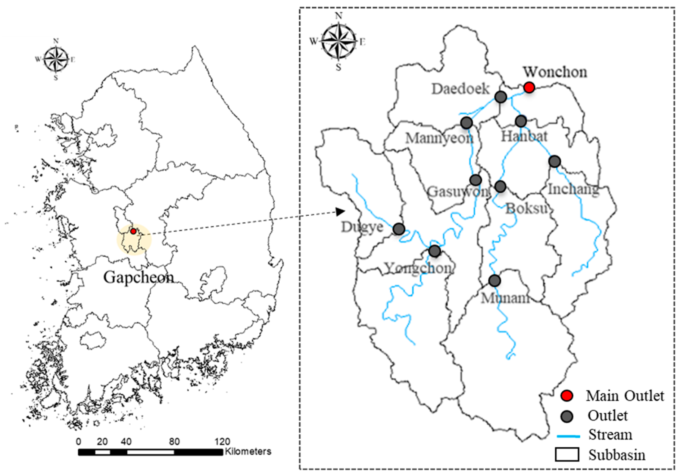
2.1. Study Watershed

The study area is the Gapcheon watershed, a subbasin of the Geum River watershed located in central South Korea, covering 602 km² (Figure 2). Moreover, the latitude is 36.37199° N, and the longitude is 127.3721° E. The Gapcheon watershed, home to approximately 1.5 million residents, has undergone significant development over the past two decades, necessitating effective water resource management [22]. In this study, land use consisted of 12.59% (75.76 km²) for urbanization, 9.31% (56.07 km²) for agriculture, 4.05% (24.39 km²) for pasture, 2.56% (15.42 km²) for paddy fields, 71.07% (428.00 km²) for forest, and 0.43% (2.59 km²) for water. Moreover, between 2008 and 2017, the study watershed received an average annual precipitation of 1231.7 mm (

Table 1. Annual precipitation and average temperatures (maximum/minimum).

Year	Annual Precipitation (mm)	Annual Temperature (°C)
		Maximum	Minimum
2008	1037.6	24.7	2.1
2009	1090.4	25.0	2.5
2010	1419.7	24.7	1.3
2011	1943.4	23.4	2.4
2012	1409.5	24.2	2.3
2013	1120.2	25.9	2.0
2014	1117.7	24.8	3.1
2015	822.7	25.4	2.7
2016	1228.4	26.4	2.6
2017	1127.5	25.3	2.3
Ave.	1231.7	25.0	2.3

), with 56.0% (689.4 mm) of the total precipitation occurring during the summer months (June to August), according to the Korea Meteorological Administration. The average annual temperature was 13.1 °C, with a maximum temperature of 25.0 °C and a minimum temperature of 2.3 °C. Streamflow data from ten monitoring stations: Gasuwon, Daedoek, Mannyeon, Dugye, Munam, Boksu, Yongchon, Inchang, Hanbat, and Wonchon were sourced from the Water Management Information System.

2.2. SWAT Overview and Input Data

SWAT is a continuous, long-term, semi-distributed model developed by the United States Department of Agriculture Research Service (USDA-ARS) to simulate at the watershed scale incorporating diverse management practices [29,30]. It achieves a balance between computational efficiency and the representation of watershed variability by using hydrologic response units (HRUs) as the foundational units for SWAT model calculations. HRUs are characterized by distinct soil combinations, land use, and slope categories within a subbasin. Additionally, in this setup, HRUs are assigned separately for each subbasin based on the specific soil, land use, and slope conditions in that subbasin. The thresholds for defining HRUs are applied in sequence to land use, soils within each land use category, and then to slopes in each combination of land use and slope [31,32]. The model simulates the hydrological cycle with hydrologic response units (HRUs) as a basic computational unit. SWAT also automatically estimates soil-related variables for each soil layer based on soil characteristic data stored in the model’s database [29]. For baseflow, SWAT assumes an aquifer system composed of both shallow and deep aquifers. The shallow aquifer contributes return flow to streams within the watershed, whereas the deep aquifer influences streams beyond the watershed boundaries [33].

Quantitative evaluation of baseflow using SWAT presents various water management strategies, including assessing the impacts of climate change on flow and baseflow variability, land use changes, and urban planning on the water cycle and analyzing the contribution of groundwater recharge and baseflow [34,35]. In this study, the Gapcheon watershed was divided into ten subbasins, considering streamflow monitoring stations, with the Wonchon station as the final outlet (Figure 2). SWAT requires various input data, including climate data, topographic data, and geographical information on land use and soil. As presented in

Table 2. Data used and corresponding sources.

Data Type	Name	Source
Meteorological data	Precipitation, wind speed, maximum and minimum temperature, relative humidity, and solar radiation	Korea Meteorological Administration (https://data.kma.go.kr/data/rmt/rmtList.do?code=400&pgmNo=570) (accessed on 15 October 2024)
Hydrological data	Daily streamflow	Water resource Management Information System (http://www.wamis.go.kr/wkw/flw_dubobsif.do) (accessed on 15 October 2024)
Spatial data	DEM	National Geographic Information Institute (https://www.ngii.go.kr/kor/content.do?sq=204) (accessed on 15 October 2024)
	Land use	Korea Ministry of Environment (https://egis.me.go.kr/req/intro.do) (accessed on 15 October 2024)
	Soil type	Korea Rural Development Administration (https://soil.rda.go.kr/soil/index.jsp) (accessed on 15 October 2024)

, the climate data were collected from the Daejeon station of the Korea Meteorological Administration (KMA) as daily data (maximum temperature, minimum temperature, humidity, wind, solar radiation, and precipitation), from 1 January 2008 to 31 December 2017. The streamflow data were obtained from the Water resource Management Information System (WAMIS), which provides daily streamflow records for ten stations (Gasuwon, Daedoek, Mannyeon, Dugye, Munam, Boksu, Yongchon, Inchang, Hanbat, and Wonchon) from 1 January 2008 to 31 December 2017. Moreover, the National Geographic Information Institute obtained the study watershed’s Digital Elevation Model (DEM) with a 10 m grid resolution. The Korea Ministry of Environment provided land use data in 2018, and the Korea Rural Development Administration obtained soil map data in 2017. The model analysis period spans eight years (2010–2017), with a 4-year warm-up period (2010–2013) based on the availability of complete streamflow data considering the period without missing streamflow data. SWAT involves numerous parameters associated with hydrologic processes, such as rainfall runoff, that require calibration to ensure accurate prediction. To calibrate streamflow predictions, we used SWAT-CUP, an automated calibration and uncertainty analysis tool, using the Sequential Uncertainty Fitting Ver.2 (SUFI-2) algorithm [36], which was selected from several available algorithms. Calibration was performed for all ten monitoring stations.

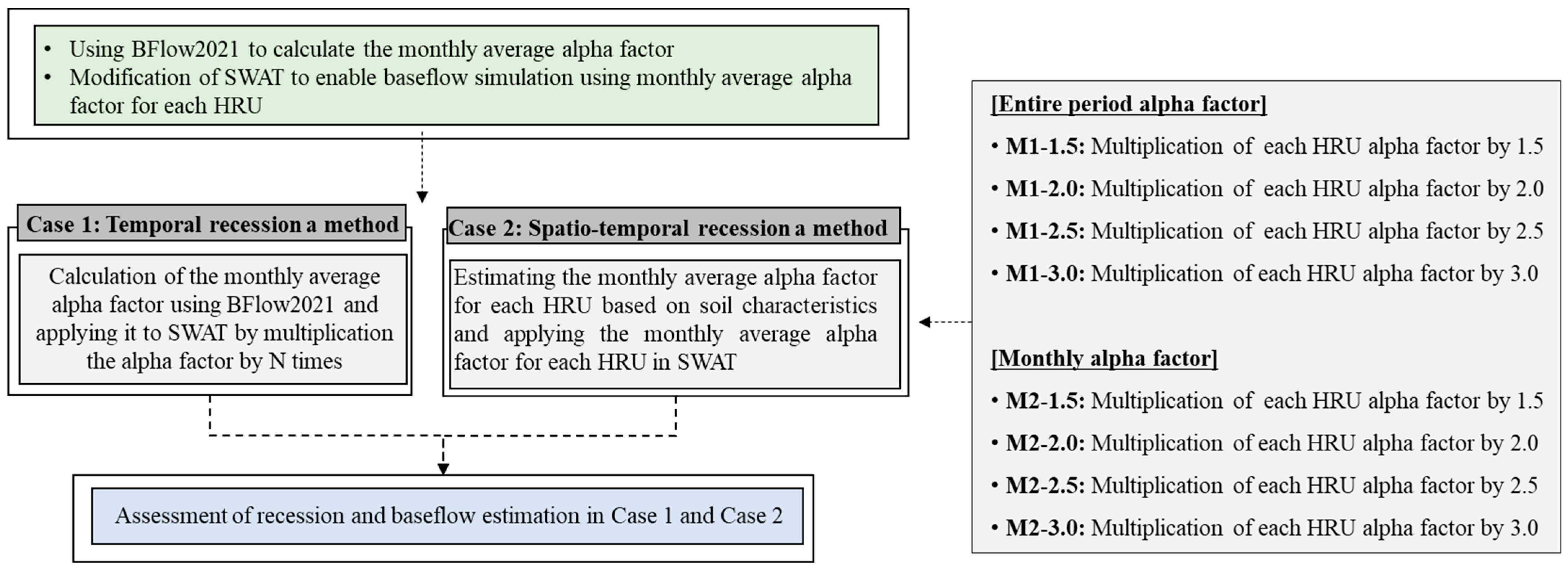
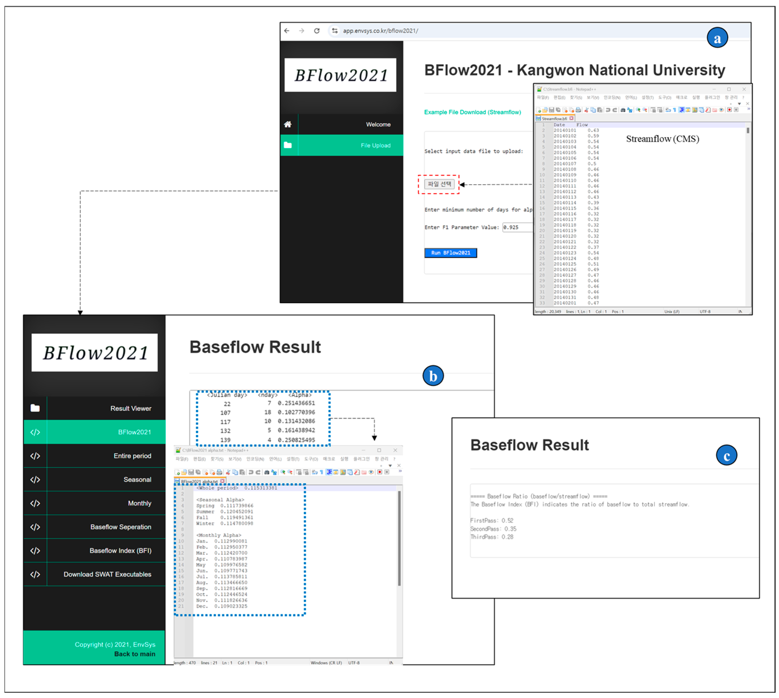
2.3. Calculating the Alpha Factor Considering Temporal and Spatial Variations

There are structural limitations in SWAT when it comes to improving baseflow prediction by identifying spatial recession characteristics for each HRU within the groundwater file. However, alpha factors related to the baseflow recession are sensitive to soil water holding capacity, area, and slope, and the distinct characteristics of each HRU within the groundwater file can be considered [37,38]. This means that when analyzing baseflow with SWAT, the soil water processes can impact baseflow. Part of the water recharged to the aquifer from the lowest soil layer moves to the deep aquifer, while the remainder recharges the shallow aquifer, where it is stored or contributes to baseflow into rivers [39,40,41]. In this regard, research is needed to consider the applicability of the alpha factor for each HRU soil column by incorporating recession characteristics into the baseflow analysis. Moreover, despite the spatial variability of these properties, no previous study has developed a method for calculating the alpha factor while accounting for these spatial heterogeneities, specifically, the HRU-specific alpha factor in SWAT. In response, this study proposes a method to calculate the HRU-specific alpha factor to consider the different recession characteristics of each HRU. In this study, calculations were performed using effective moisture content and soil layer depth data, taking into account the characteristics of the soil profiles. Soil properties and types were determined from the soil map for each subbasin to represent the soil characteristics. The calculations were made by multiplying the depth of each soil layer by the available water capacity (AWC) for each soil type and then summing the results to the soil depth and characteristics of each layer. AWC, which represents the available moisture content in each soil layer, is calculated by subtracting the moisture content at the permanent wilting point from the field capacity [42]. In this study, the total storage capacity was determined using soil type data. Since it pertains to the water storage potential in the deeper soil layers, smaller values reflect a reduced capacity for water retention. In contrast, larger values indicate higher water storage capacity, and they also have a more significant impact on the sensitivity of the alpha factor. Additionally, this study assumed that the alpha factor is more sensitive when the area of each HRU is large and the slope is gentle. Considering these factors, each HRU within the subbasin was classified, and alpha factor values were assigned accordingly.

2.4. Validation of the Effect of the Spatial and Temporal Alpha Factors on Recession Simulation

Given the temporal impact on recession characteristics demonstrated by Lee et al. [28], we set several scenarios (

Table 3. Diverse methods for comprehensive evaluation of the effectiveness of the spatial, temporal, and spatiotemporal alpha factor in simulating streamflow recession. ‘Entire’ denotes the alpha factor estimated over the entire observation period, while ‘Monthly’ refers to calculations performed on a monthly basis. Each method applies a specific multiplier, ranging from 1.5 to 3.0, to the optimal value to define the range of the alpha factor applied to the HRUs.

Section	Method	Temporal Extent	Spatial Extent	Multiplier
Case 1	Baseline	Monthly	Subbasin	2.0–3.0
Case 2	M1–1.5	Entire	HRU	1.5
	M1–2.0	Entire	HRU	2.0
	M1–2.5	Entire	HRU	2.5
	M1–3.0	Entire	HRU	3.0
	M2–1.5	Monthly	HRU	1.5
	M2–2.0	Monthly	HRU	2.0
	M2–2.5	Monthly	HRU	2.5
	M2–3.0	Monthly	HRU	3.0

) to comprehensively evaluate the effects of temporal and spatial variations on recession and baseflow simulation. For temporal influence assessment, we compared a single, long-term average alpha factor for the entire simulation period with monthly alpha factors. Baseflow is typically associated with aquifer characteristics, so the master recession curve (MRC) in a single exponential is utilized to calculate the alpha factor from BFlow. However, since BFlow provides users with a single alpha factor, it is essential to take into account the temporal characteristics of baseflow recession, given its distinct seasonal climate and substantial flow variations in South Korea. In other words, it is challenging to represent the complex streamflow characteristics using a single value for the whole period. To address this issue, the monthly alpha coefficients were calculated using BFlow2021, modified by Lee [28] (https://app.envsys.co.kr/bflow2021/) (accessed on 15 October 2024) (Figure 3). BFlow2021 enables users to automatically download the calculated monthly and seasonal alpha factors after inputting daily streamflow data.

For spatial influence evaluation, the HRU-specific alpha factor was calculated based on the proposed method by this study, as explained in the previous section. Lee et al. [26] and Lee et al. [27] stated that the alpha factor calculated from BFlow should be recalibrated to increase the accuracy of the recession simulation. However, Lee [28] found that multiplying the alpha factor from BFlow by 2.0–2.5 times showed a better match between observed and simulated recession, but only considering the temporal variations of the recession characteristics. Therefore, this study tested different multipliers from 1.5 to 3.0 to find an optimal value for the spatiotemporal alpha factor application. These multipliers were multiplied to the optimal alpha factor value calculated from BFlow2021 (long-term average and monthly values). Case 1 applies the monthly average alpha factor, estimated using BFlow2021, to the SWAT. This study proposed different methods (M1s, M2s) in Case 2 to determine the most effective way to apply the differential alpha factor at each HRU. By combining various conditions, a total of eight cases were compared, as shown in Table 3. The baseline model only considers the temporal variation in recession (monthly alpha factor), M1s only consider the spatial variation (HRU-specific alpha factor), and M2s apply the spatiotemporal variations (monthly, HRU-specific alpha factor). The numbers from 1.5 to 3.0 behind M1 and M2 represent multipliers to the optimal value to define the range of the alpha factor applied to HRUs within each subbasin. In this study, the SWAT was modified by adjusting the Fortran code to enable the application of the alpha factor across both spatial and temporal scales.

2.5. Assessment of Recession and Baseflow Estimation in Case 1 and Case 2

This study used SWAT-CUP to calibrate streamflow to evaluate baseflow and recession in nine subbasins and one watershed across both Case 1 and Case 2. Case 1 applied the monthly average alpha factor for each subbasin, considering the temporal recession method in this study. In contrast, in Case 2, the method applied from M1s to M2s (the previously mentioned) applied the monthly average alpha factor by HRU for each subbasin, considering the spatiotemporal recession method. After calibration using SWAT-CUP, the alpha factors for Case 1 and Case 2 were as fixed parameters and applied in SWAT to predict recession characteristics. In this study, the performance assessment for the model’s performance is evaluated using several metrics, including Nash–Sutcliffe Efficiency (NSE), the Coefficient of Determination (R²), the Index of Agreement (IOA), Percent Bias (PBIAS), and Mean Absolute Percentage Error (MAPE) [43] (Equations (1) to (5)). Baseflow reflecting recession characteristics was analyzed using Pass 1 of BFlow2021, which separated it from the observed streamflow in study watersheds. Moreover, the BFI, representing the contribution of baseflow to the streamflow, was computed for each of the study watersheds. To compare the observed streamflow with the baseflow calculated using BFlow2021, the streamflow simulated by SWAT (Case 1 and Case 2) was separated into baseflow using BFlow2021. In this study, to evaluate the improvement of the baseflow recession prediction in models in Case 1 and Case 2, the observed recession was extracted and compared with the simulated recession.

$$NSE=1-\left[{\displaystyle \frac{{\sum }_{i=1}^n{(y_{obs,i}-y_{sim,i})}^2}{{\sum }_{i=1}^n{(y_{obs,i}-{\overline{Y}}_{obs})}^2}}\right]$$

(1)

$$R^2={\displaystyle \frac{({\sum }_{i=1}^n(y_{obs,i}-{\overline{Y}}_{obs }){(y_{sim,i}-{\overline{Y}}_{sim }))}^2}{{\sum }_{i=1}^n{(y_{obs,i}-{\overline{Y}}_{obs})}^2\sum _{i=1}^n{(y_{sim,i}-{\overline{Y}}_{sim })}^2}}$$

(2)

$$IOA=1-\left[{\displaystyle \frac{{\sum }_{i=1}^n{(y_{obs,i}-y_{sim,i})}^2}{{\sum }_{i=1}^n{(\left|y_{sim,i}-{\overline{Y}}_{obs }\right|+\left|y_{obs,i}-{\overline{Y}}_{obs }\right|)}^2}}\right]$$

(3)

$$PBIAS=100\times \left[{\displaystyle \frac{{\sum }_{i=1}^n(y_{obs,i}-y_{sim,i}) }{{\sum }_{i=1}^n{y}_{obs,i}}}\right]$$

(4)

$$MAPE={\displaystyle \frac{100}{n}}{\sum }_{i=1}^n\left[{\displaystyle \frac{y_{obs,i}-y_{sim,i}}{y_{obs,i}}}\right]$$

(5)

where $y_{obs,i}$ (m³/s) is the observation, $y_{sim,i}$ (m³/s) is the simulation, ${\overline{Y}}_{obs}$(m³/s) is the mean of the observations, ${\overline{Y}}_{obs}$ (m³/s) is the mean of the simulations, and $n$ is the total number of observations.

3. Results and Discussion

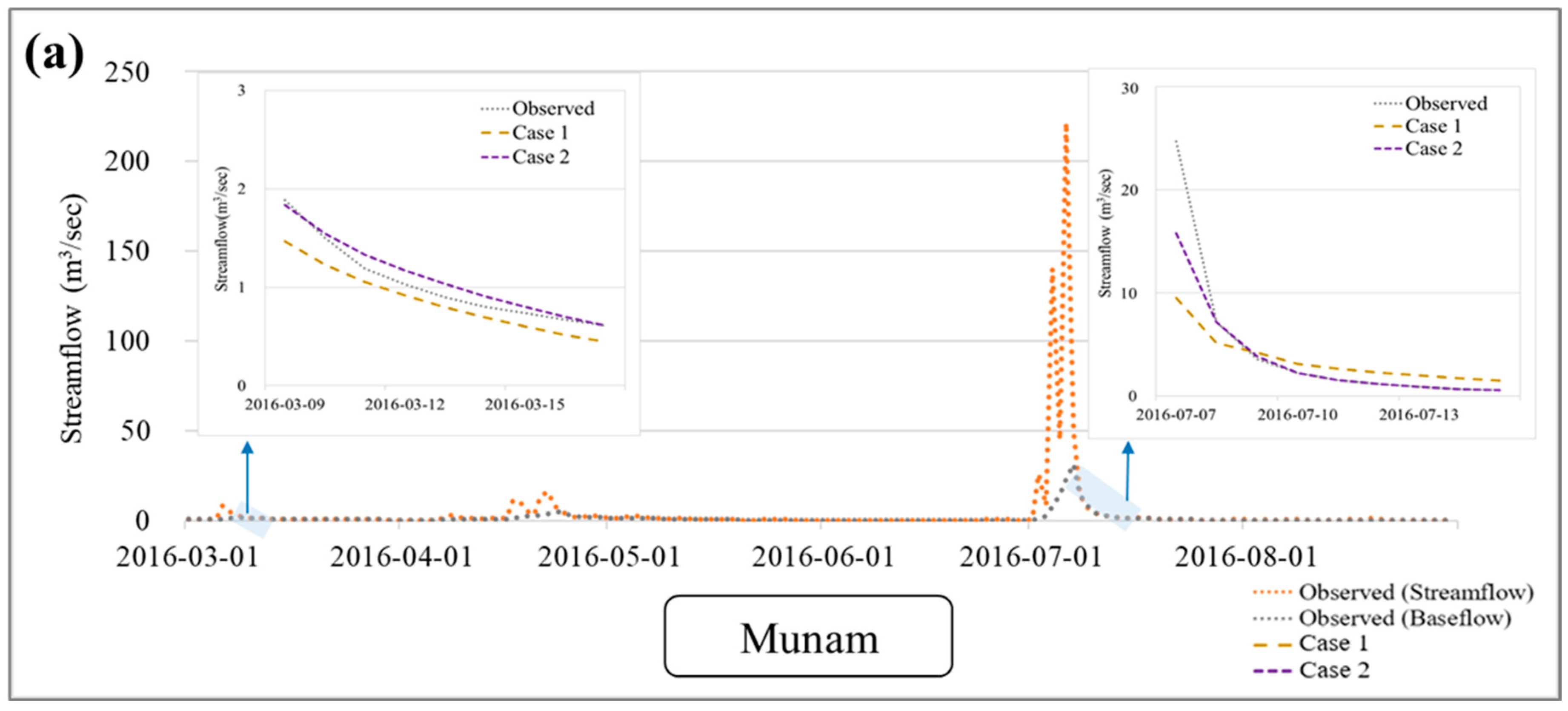
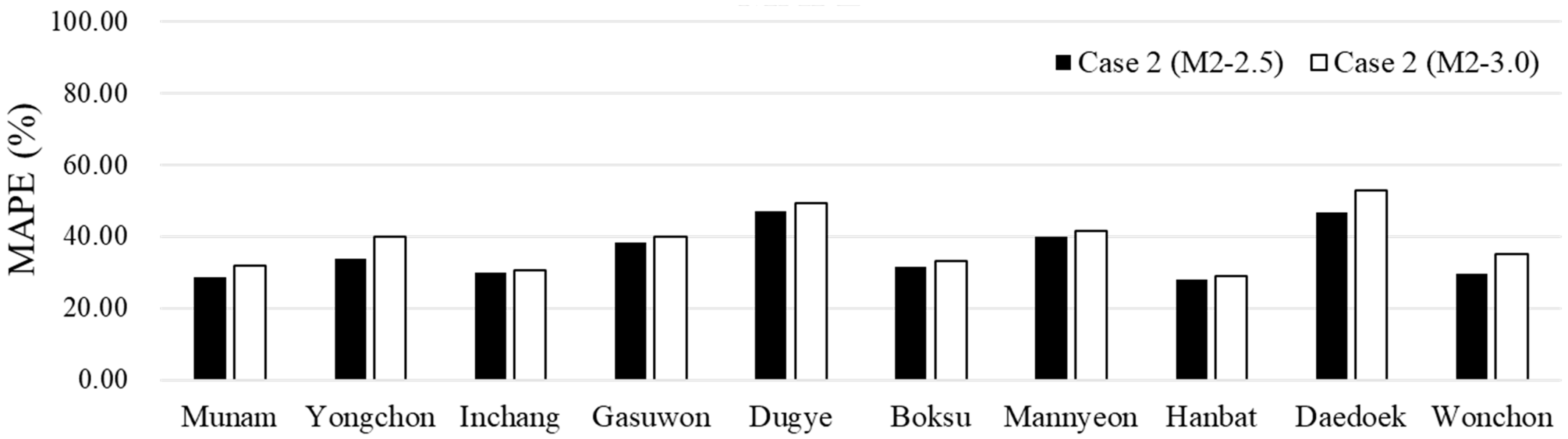
3.1. Comparison of Recession Estimation in Case 1 and Case2

Before evaluating the baseflow prediction of Case 1 and Case 2, it is necessary to assess whether the model accurately simulates streamflow results.

Table 4. Model performance results for daily streamflow of the study watersheds.

Study Watershed	NSE	R2	IOA	PBIAS (%)	MAPE (%)
Munam	0.56	0.56	0.84	9.51	68.97
Yongchon	0.57	0.58	0.83	21.54	66.17
Inchang	0.56	0.57	0.82	9.66	72.51
Gasuwon	0.62	0.63	0.88	−8.36	57.71
Dugye	0.73	0.78	0.93	35.26	65.47
Boksu	0.62	0.66	0.90	−8.82	68.63
Mannyeon	0.64	0.66	0.86	7.25	65.16
Hanbat	0.58	0.57	0.86	12.92	63.02
Daedoek	0.57	0.64	0.83	43.98	76.63
Wonchon	0.53	0.54	0.84	−0.63	67.32

presents the calibration results for the streamflow estimated using Case 1 in this study. For the SWAT calibration assessment by Moriasi et al. [43], the NSE was evaluated as ‘satisfactory’ (NSE > 0.5). Moreover, as the IOA approaches 1, it indicates a higher level of agreement between the model predictions and the observed data. The IOA results also indicate high streamflow simulation predictions for the nine subbasins and the one watershed. The remaining evaluation metrics, R² and PBIAS, also indicate that the model calibration was generally well performed. Specifically, for the Munam, Inchang, and Mannyeon watersheds, positive PBIAS values (9.51%, 9.66%, and 7.25%, respectively) indicate that the model shows a slight underestimation of the observed values. On the other hand, the Gasuwon watershed has a negative PBIAS of −8.36%, indicating that the model slightly overestimates the observed values. These PBIAS values, along with the R² values, support the conclusion that the model calibration achieved a reasonable level of accuracy. Moreover, Table 4 indicates that the provided explanation emphasizes the importance of using multiple evaluation metrics to assess model performance comprehensively. In the case of Dugye, while the NSE value of 0.73 indicates satisfactory calibration and is the highest among the ten study watersheds, and the IOA of 0.93 suggests a strong agreement between model predictions and observed data, these metrics alone do not provide the complete view of model accuracy. The high PBIAS of 35.26% reveals a significant bias in the model’s predictions, indicating that despite the satisfactory NSE and IOA values, the model either consistently overestimates or underestimates the observed values. This discrepancy highlights that even when metrics like NSE and IOA suggest good performance, a PBIAS can uncover areas where the model’s accuracy is lacking, reinforcing the need to use multiple metrics for a thorough evaluation of model performance.

Among the M1s that applied the average long-term alpha factor for each HRU, M1–2.5, which is the result of multiplying the optimal value by 2.5, showed better predictive performance. Although its overall prediction accuracy was lower compared to Case 1 in terms of comprehensive evaluation metrics, this indicates that Case 2 (M1–2.5) has a prediction trend more similar to the observed recession than other M1s. Moreover, when comparing the results from Case 1 (baseline) with M1–2.5, it was evaluated that there was no improvement at multiple stations, and the overall NSE and MAPE predictability decreased (

Table 5. Comparison of simulated recessions in Case 1 and Case 2 (M1–2.5) and observed recession.

Study Watershed	NSE		R2		IOA		PBIAS (%)		MAPE (%)
	Case 1	Case 2 (M1–2.5)	Case 1	Case 2 (M1–2.5)	Case 1	Case 2 (M1–2.5)	Case 1	Case 2 (M1–2.5)	Case 1	Case 2 (M1–2.5)
Munam	0.58	0.58	0.70	0.74	0.82	0.81	23.22	22.75	30.22	32.38
Yongchon	0.61	0.58	0.66	0.68	0.86	0.84	20.27	22.11	37.98	38.24
Inchang	0.64	0.64	0.87	0.87	0.84	0.83	23.52	21.95	32.38	29.89
Gasuwon	0.63	0.73	0.71	0.79	0.88	0.91	-28.19	-17.07	42.65	38.96
Dugye	0.57	0.52	0.58	0.54	0.85	0.86	-4.72	0.31	49.92	50.98
Boksu	0.66	0.64	0.86	0.86	0.85	0.83	19.01	18.92	32.94	32.73
Mannyeon	0.56	0.54	0.66	0.68	0.80	0.77	-8.53	-2.82	42.93	56.34
Hanbat	0.70	0.69	0.77	0.77	0.89	0.88	13.33	14.63	30.06	33.15
Daedoek	0.50	0.45	0.53	0.61	0.75	0.72	-47.10	-24.09	51.61	61.88
Wonchon	0.70	0.69	0.79	0.87	0.87	0.86	-3.50	-0.50	33.85	33.39

, Figure 4). In Figure 4, MAPE provides a clear and intuitive measure of the model’s prediction accuracy by expressing errors as a percentage. This makes it easier to understand the relative size of the prediction errors, regardless of the scale of the data. Unlike PBIAS, which can be sensitive to the sign and magnitude of the errors, MAPE focuses on absolute errors, offering a balanced view of model performance across different datasets. In other words, MAPE was indicated to the overall prediction accuracy without being overly affected by individual overestimations or underestimations. Additionally, the NSE values generally worsened across study watersheds (Dugye, Yongchon, Boksu, Mannyeon, Hanbat, Daedoek, and Wonchon), with the exception of Munam and Inchang, which remained unchanged. While the PBIAS values ideally should decrease as they approach zero, the outcomes were different: the PBIAS values for most watersheds, including Munam, Inchang, Gasuwon, Dugye, Boksu, Mannyeon, Daedoek, and Wonchon, actually decreased, indicating an improvement, whereas only Yongchon and Hanbat showed an increase. The lack of improvement in MAPE results and the significant estimation uncertainty are presumed to be due to applying a uniform alpha factor from the M1s distribution. In this context, MAPE, which is Mean Absolute Percentage Error, measures the accuracy of the model by quantifying how closely the predicted values align with the observed data. A lack of improvement in MAPE indicates that the model’s predictions are still showing considerable deviation from the actual values, suggesting that the use of a uniform alpha factor in the entire period may not be suitable for effectively predicting the variations within the recession. In other words, the methodology adopted from M1s is unsuitable for the intended simulations.

On the other hand, M2s, which apply the monthly alpha factor for each HRU, improved the predictions of the recession simulations compared to the baseline model, with a decrease in MAPE errors (

Table 6. Comparison of simulated recessions in Case 1 and Case 2 (M2–2.5) and observed recession.

Study Watershed	NSE		R2		IOA		PBIAS (%)		MAPE (%)
	Case 1	Case 2 (M2–2.5)	Case 1	Case 2 (M2–2.5)	Case 1	Case 2 (M2–2.5)	Case 1	Case 2 (M2–2.5)	Case 1	Case 2 (M2–2.5)
Munam	0.58	0.58	0.70	0.72	0.82	0.82	23.22	23.16	30.22	28.66
Yongchon	0.61	0.61	0.66	0.70	0.86	0.85	20.27	17.00	37.98	33.68
Inchang	0.64	0.65	0.87	0.87	0.84	0.84	23.52	22.20	32.38	29.88
Gasuwon	0.63	0.69	0.71	0.76	0.88	0.90	−28.19	−22.62	42.65	38.51
Dugye	0.57	0.60	0.58	0.68	0.85	0.88	−4.72	−18.40	49.92	46.94
Boksu	0.66	0.66	0.86	0.86	0.85	0.85	19.01	18.31	32.94	31.69
Mannyeon	0.56	0.57	0.66	0.68	0.80	0.80	−8.53	−8.05	42.93	40.08
Hanbat	0.70	0.72	0.77	0.78	0.89	0.89	13.33	10.79	30.06	27.88
Daedoek	0.50	0.53	0.53	0.53	0.75	0.75	−47.10	−36.78	51.61	46.88
Wonchon	0.70	0.74	0.79	0.84	0.87	0.90	−3.50	−8.47	33.85	29.48

, Figure 5). Moreover, the enhancement in model predictions was demonstrated in the results of other performance criteria. For NSE, predictions improved for all watersheds except for Munam, Yongchon, and Boksu, while for R², improvements were indicated in all watersheds except for Inchang, Boksu, and Daedoek. Table 6 shows that in the Dugye and Wonchon watersheds, the PBIAS values in Case 2 (M2–2.5) are worse than in Case 1, indicating increased bias in the simulated prediction results. The negative PBIAS in Case 2 indicates greater overestimation, warranting further supplement into potential causes, such as specific periods or conditions where the model may overestimate. However, in this study, other performance metrics such as NSE, R², and IOA show improvements in Case 2, suggesting that the model better predicts the overall spatial–temporal variability of the observed recession despite the increased bias. In other words, given that this study focuses on accurately simulating recession, the improved NSE, R², and IOA in Case 2 indicate better performance in this regard. This trade-off should be carefully considered in future studies when evaluating model performance.

Figure 6 shows the baseflow recession of a representative upstream and downstream point out of the ten stations. The performance trend in M2–2.5 showed similarities to the observation recession compared to Case 1. This indicates that the approach in Case 2, which incorporates spatial characteristics alongside the application of monthly alpha factor, is a more effective analysis method compared to the approach used in Case 1. When applying the alpha factor on an HRU basis, utilizing a methodology that maintains the ratio within each HRU at less than twice the average resulted in a lower improvement than Case 1. These findings suggest that Case 2 (M2–2.5), which typically involves the multiplication of the alpha factor by an average factor of 2.5, primarily enhances the simulation results of recession characteristics. These findings suggest that instead of applying a uniform alpha factor for the entire duration, it is advisable to consider applying monthly average alpha factor values.

An additional comparative analysis of the recession curve was conducted for M2–2.5 and M2–3.0 in Case 2. The only difference between M2–2.5 and M2–3.0 is that the maximum range for M2–3.0 was set to 3. As shown in

Table 7. Comparison of simulated recessions in Case 2 (M2–2.5, M2–3.0) observed recession.

Study Watershed	NSE		R2		IOA		PBIAS (%)		MAPE (%)
	M2–2.5	M2–3.0	M2–2.5	M2–3.0	M2–2.5	M2–3.0	M2–2.5	M2–3.0	M2–2.5	M2–3.0
Munam	0.58	0.54	0.72	0.62	0.82	0.80	23.16	13.93	28.66	31.82
Yongchon	0.61	0.58	0.70	0.64	0.85	0.86	17.00	13.59	33.68	39.94
Inchang	0.65	0.59	0.87	0.69	0.84	0.83	22.20	16.28	29.88	30.75
Gasuwon	0.69	0.52	0.76	0.66	0.90	0.86	−22.62	−26.51	38.51	40.05
Dugye	0.60	0.52	0.68	0.56	0.88	0.77	−18.40	6.30	46.94	49.41
Boksu	0.66	0.57	0.86	0.60	0.85	0.83	18.31	6.34	31.69	33.21
Mannyeon	0.57	0.63	0.68	0.73	0.80	0.84	−8.05	−21.04	40.08	41.57
Hanbat	0.72	0.52	0.78	0.53	0.89	0.84	10.79	8.77	27.88	29.12
Daedoek	0.53	0.50	0.53	0.68	0.75	0.79	−36.78	−55.47	46.88	52.94
Wonchon	0.74	0.65	0.84	0.70	0.90	0.87	−8.47	−10.32	29.48	35.17

and Figure 7, the improvement rate of MAPE in M2–3.0 was lower than in M2–2.5. Moreover, M2–2.5 presented results that showed a decrease in model predictability and increased uncertainty from the upstream to the downstream locations across different performance criteria. As a result, at the main outlet, Wonchon, M2–3.0 indicates a significant difference compared to M2–2.5. This means that the differences between M2–2.5 and M2–3.0 at Wonchon indicate that M2–3.0 results in a decline in performance across multiple metrics, including increased bias and error. These differences suggest that M2–2.5 provides more accurate predictions and a better fit for the observed recession in Wonchon. Therefore, M2–2.5 appears to be the preferable method for this watershed when the goal is to minimize overestimation and ensure more reliable recession predictions.

This indicates that a more extensive range for HRU-specific alpha factor application does not necessarily lead to selecting the optimal alpha factor application method. Moreover, the comparison assessment between M2–3.0 and Case 1 (baseline) did not show improved predictive performance across all study watersheds. These results are similar to the results observed when applying the optimal alpha factor range of 2.57, as proposed by Lee et al. [24] for the same study area in the Gapcheon watershed.

Additionally, Lee et al. [26] and Lee et al. [27] found that multiplying the alpha factor of BFlow in the SWAT groundwater input file (.gw) by 2.0 to 2.5 times the average HRU-specific alpha factor is the optimal range for improving SWAT’s recession and baseflow predictions for various study areas in South Korea. Therefore, the optimal range for applying the alpha factor in the study area was established, applied, and analyzed, and it was evaluated across M1s and M2s. This study established a suitable range for the alpha factor by considering various factors to reflect the spatiotemporal sensitivity characteristics. However, further refinement is needed to account for various soil factors, such as hydraulic conductivity and organic matter content. Future research should consider these aspects when estimating the monthly average alpha factor for each HRU.

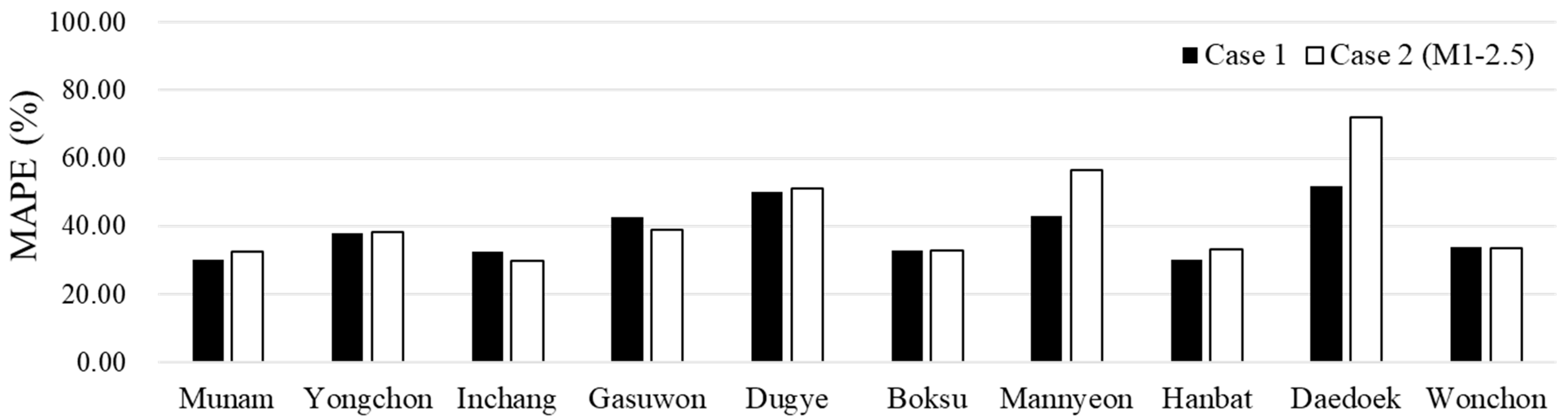
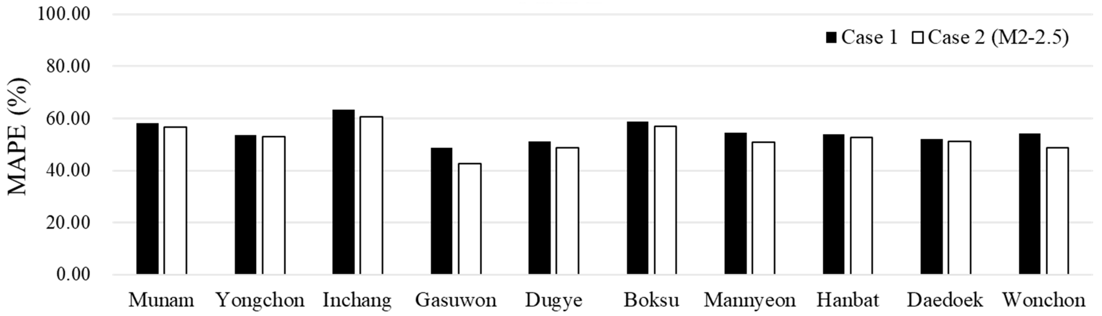
3.2. Comparison of Baseflow Estimation in Case 1 and Case 2

After evaluating the recession simulations from M1s to M2s in Case 2 compared to Case 1, the baseflow was evaluated for the optimal approach in Case 2 (M2–2.5) (

Table 8. Comparison of baseflow results for each case against observed baseflow after separating baseflow from both observed and SWAT streamflow using BFlow2021.

Study Watershed	NSE		R2		IOA		PBIAS (%)		MAPE (%)
	Case 1	Case 2 (M2–2.5)	Case 1	Case 2 (M2–2.5)	Case 1	Case 2 (M2–2.5)	Case 1	Case 2(M2–2.5)	Case 1	Case 2 (M2–2.5)
Munam	0.65	0.65	0.67	0.67	0.87	0.87	23.80	23.11	58.10	56.72
Yongchon	0.55	0.57	0.61	0.62	0.87	0.87	25.01	23.06	53.69	52.86
Inchang	0.64	0.64	0.68	0.68	0.88	0.89	31.31	31.12	63.35	60.68
Gasuwon	0.54	0.54	0.67	0.67	0.90	0.90	−4.61	−5.51	48.59	42.50
Dugye	0.53	0.54	0.57	0.57	0.85	0.86	17.49	17.44	51.31	57.06
Boksu	0.64	0.64	0.65	0.65	0.89	0.89	16.70	16.22	58.70	50.96
Mannyeon	0.62	0.61	0.63	0.62	0.88	0.88	−0.41	−1.13	54.64	52.77
Hanbat	0.53	0.54	0.60	0.60	0.87	0.87	27.32	27.14	53.78	51.10
Daedoek	0.52	0.52	0.54	0.54	0.83	0.83	20.93	20.07	52.07	51.10
Wonchon	0.67	0.68	0.67	0.68	0.89	0.90	4.80	1.41	54.26	48.69

). Similar to the trends observed in the simulations, the results of Case 2 (M2–2.5) showed improvement compared to Case 1 in baseflow results. In particular, in Case 2 (M2–2.5), there was a decrease in MAPE error rates, resulting in better results (Figure 8). Moreover, PBIAS exhibited trends similar to those observed in the data. The comprehensive results of recession and baseflow simulations indicate that when applying the monthly average alpha factor by HRU in SWAT, ensuring the reliability of model results requires an average application of more than 2.5 times the baseline value. This study improved the simulation analysis of baseflows at specific stations by differentially applying HRU-specific alpha factors rather than a uniform application across all HRUs.

The variation in alpha factor values across HRUs is influenced by a specific area, soil type, and slope, which dictate baseflow recession moves through the watershed. For instance, permeable soils may require a lower alpha factor to account for slower recession, while steeper slopes may necessitate higher values due to faster runoff. This differentiation across HRUs is key to improving model accuracy. Moreover, this method calculates the alpha factor through BFlow2021 based on measured flows and can also be applicable at ungauged stations. However, since this study focused on alpha factor application methods considering recession characteristics, other parts of the hydrograph were not fully accounted for. In other words, while the simulated recession showed high predictability, the baseflow predictions did not see significant improvement comparatively. Furthermore, in this study, the optimal approach, Case 2 (M2–2.5), involved using the monthly average alpha coefficient for each HRU to improve prediction modeling capabilities in both recession and baseflow simulations. In future studies, it is proposed that this approach be applied as training and validation data through machine learning to enhance the usability of the model for users. Machine learning can be trained using the available results from well-predicted watersheds in this study and then used to predict the hydrological behavior of ungauged stations with insufficient observational data. Through this, machine learning can be integrated into decision support systems, making them easy to use and accessible to non-experts. By providing easily interpretable results, machine learning-based models can assist water resource managers in making informed decisions. Moreover, incorporating machine learning into hydrological modeling presents an opportunity to enhance the predictive efficiency, accuracy, and user-friendliness of models.

4. Conclusions

The existing alpha factor calculation method in SWAT was limited by its inability to consider spatial–temporal variations, affecting its accuracy in predicting recession and baseflow. To address this, the study proposed a method to calculate and apply spatial–temporal alpha factors to improve SWAT’s predictability and accuracy, with a focus on recession and baseflow simulations. Case 1 indicates that it has been modified to BFlow2021 and SWAT to enable the application of monthly alpha factors, considering various streamflow conditions for temporal recession characteristics. However, applying HRU-specific alpha factors at ungauged stations remained a challenge. Case 2 aimed to overcome this by incorporating both spatial and temporal characteristics when calculating alpha factors. The alpha factor values for each HRU were prioritized according to factors reflecting soil characteristics, slope, and area. The alpha factor values were linearly set from M1s to M2s for each HRU. The optimal method was determined by comparing the spatial–temporal alpha factor application from M1s to M2s with the monthly average alpha factor (Case 1). Case 2 (M2–2.5), which considers the application of the monthly average alpha factor for each HRU, shows improvement and a reduction in error rates compared to Case 1, as indicated by the statistical metrics. Moreover, these results are crucial for developing watershed-based baseflow management standards and can be applied to ungauged stations. Since baseflow contributes to water quality issues like nitrate pollution, spatial and temporal baseflow predictions can aid in preemptive water quality management, and future research will validate this approach across various watersheds.

References

1. Wang, W.; Wang, S. Sustainable Stormwater Management for Different Types of Water-Scarce Cities: Environmental Policy Effect of Sponge City Projects in China. Sustainability 2024, 16, 5685. [Google Scholar] [CrossRef]
2. Lee, G.J.; Park, K.W.; Jung, Y.H.; Jung, I.K.; Jung, K.W.; Jeon, J.H.; Lee, J.M.; Lim, K.J. Analysis of flood control effects of heightening of agricultural reservoir dam. J. Korean Soc. Agric. Eng. 2013, 55, 83–93. [Google Scholar]
3. Miller, O.L.; Miller, M.P.; Longley, P.C.; Alder, J.R.; Bearup, L.A.; Pruitt, T.; Jones, D.K.; Putman, A.L.; Rumsey, C.A.; McKinney, T. How Will Baseflow Respond to Climate Change in the Upper Colorado River Basin? Geophys. Res. Lett. 2021, 48, e2021GL095085. [Google Scholar] [CrossRef]
4. Wu, G.; Zhang, J.; Li, Y.; Liu, Y.; Ren, H.; Yang, M. Revealing Temporal Variation of Baseflow and Its Underlying Causes in the Source Region of the Yangtze River (China). Hydrol. Res. 2024, 55, 392–411. [Google Scholar] [CrossRef]
5. Bicknell, B.R.; Imhoff, J.C.; Kittle, J.L., Jr.; Donigian, A.S., Jr.; Johanson, R.C. Hydrological Simulation Program—FORTRAN, User’s Manual for Version 11; U.S. Environmental Protection Agency, National Exposure Research Laboratory: Athens, GA, USA, 1997. [Google Scholar]
6. Gironás, J.; Roesner, L.A.; Rossman, L.A.; Davis, J. A new applications manual for the Storm Water Management Model(SWMM). Environ. Model. Softw. 2010, 25, 813–814. [Google Scholar] [CrossRef]
7. Tufekcioglu, M.; Yavuz, M.; Zaimes, G.N.; Dinc, M.; Koutalakis, P.; Tufekcioglu, A. Application of Soil Water Assessment Tool (SWAT) to suppress wildfire at Bayam Forest, Turkey. J. Environ. Biol. 2017, 38, 719–726. [Google Scholar] [CrossRef]
8. Koutalakis, P.; Vlachopoulou, A.; Emmanouloudis, D.; Zaimes, G.N. Simulation of torrent discharge using SWAT and evaluation by field survey in Thasos Island. J. Eng. Sci. Technol. Rev. 2017, 10, 7–10. [Google Scholar] [CrossRef]
9. Koutalakis, P.; Zaimes, G.N.; Loannou, K.; Lakovoglou, V. Application of the SWAT model on torrents of the Menoikio, Greece. Fresenius Environ. Bull. 2017, 26, 1210–1215. [Google Scholar]
10. Pushpalatha, R.; Perrin, C.; Le Moine, N.; Andréassian, V. A Review of Efficiency Criteria Suitable for Evaluating Low-Flow Simulations. Journal of Hydrology 2012, 420–421, 171–182. [Google Scholar] [CrossRef]
11. Parra, V.; Arumí, J.L.; Muñoz, E. Identifying a Suitable Model for Low-Flow Simulation in Watersheds of South-Central Chile: A Study Based on a Sensitivity Analysis. Water 2019, 11, 1506. [Google Scholar] [CrossRef]
12. Price, K.; Jackson, C.R.; Parker, A.J.; Reitan, T.; Dowd, J.; Cyterski, M. Effects of Watershed Land Use and Geomorphology on Stream Low Flows during Severe Drought Conditions in the Southern Blue Ridge Mountains, Georgia and North Carolina, United States. Water Resour. Res. 2011, 47, 1–19. [Google Scholar] [CrossRef]
13. Lei, Y.; Jiang, X.; Geng, W.; Zhang, J.; Zhao, H.; Ren, L. The Variation Characteristics and Influencing Factors of Base Flow of the Hexi Inland Rivers. Atmosphere 2021, 12, 356. [Google Scholar] [CrossRef]
14. Kang, H.; Hyun, Y.J.; Jun, S.M. Regional estimation of baseflow index in Korea and analysis of baseflow effects according to urbanization. J. Korea Water Resour. Assoc. 2019, 52, 97–105. [Google Scholar]
15. Choi, S.-H.; Kim, S.-H.; Kim, K. Assessment for the Possibility of Water-Ecosystem Restoration Applying LID Techniques in the Deokjin Park Area, Jeonju City. Econ. Environ. Geol. 2015, 48, 477–490. [Google Scholar] [CrossRef]
16. Lamichhane, M.; Phuyal, S.; Mahato, R.; Shrestha, A.; Pudasaini, U.; Lama, S.D.; Chapagain, A.R.; Mehan, S.; Neupane, D. Assessing Climate Change Impacts on Streamflow and Baseflow in the Karnali River Basin, Nepal: A CMIP6 Multi-Model Ensemble Approach Using SWAT and Web-Based Hydrograph Analysis Tool. Sustainability 2024, 16, 3262. [Google Scholar] [CrossRef]
17. Biagi, K.M.; Ross, C.A.; Oswald, C.J.; Sorichetti, R.J.; Thomas, J.L.; Wellen, C.C. Novel Predictors Related to Hysteresis and Baseflow Improve Predictions of Watershed Nutrient Loads: An Example from Ontario’s Lower Great Lakes Basin. Sci. Total Environ. 2022, 826, 154023. [Google Scholar] [CrossRef]
18. Cao, W.; Li, Q.; Xu, H.; Zhang, Z. Vegetation Dynamics Regulate Baseflow Seasonal Patterns of the Chaohe Watershed in North China. J. Hydrol. Reg. Stud. 2024, 53, 101797. [Google Scholar] [CrossRef]
19. Anderson, M.G.; Burt, T.P. Interpretation of Recession Flow. J. Hydrol. 1980, 46, 89–101. [Google Scholar] [CrossRef]
20. Rutledge, A. Computer Programs for Describing the Recession of Ground-Water Discharge and for Estimating Mean Ground-Water Recharge and Discharge from Streamflow Records: Update No. 98; U.S. Geological Survey: Reston, VA, USA, 1998. [Google Scholar]
21. Arnold, J.G.; Allen, P.M. Automated Methods for Estimating Baseflow and Ground Water Recharge from Streamflow Records. JAWRA J. Am. Water Resour. Assoc. 1999, 35, 411–424. [Google Scholar] [CrossRef]
22. Sloto, R.A.; Crouse, M.Y.; Eaton, G.P. HYSEP: A Computer Program for Streamflow Hydrograph Separation and Analysis; U.S. Geological Survey: Reston, VA, USA, 1996. [Google Scholar]
23. Kyoung, J.L.; Engel, B.A.; Tang, Z.; Choi, J.; Kim, K.S.; Muthukrishnan, S.; Tripathy, D. Automated Web GIS Based Hydrograph Analysis Tool, WHAT. JAWRA J. Am. Water Resour. Assoc. 2005, 41, 1407–1416. [Google Scholar] [CrossRef]
24. Luo, Z.; Shao, Q. A Modified Hydrologic Model for Examining the Capability of Global Gridded PET Products in Improving Hydrological Simulation Accuracy of Surface Runoff, Streamflow and Baseflow. J. Hydrol. 2022, 610, 127960. [Google Scholar] [CrossRef]
25. Duan, H.; Li, L.; Kong, Z.; Ye, X. Combining the Digital Filtering Method with the SWAT Model to Simulate Spatiotemporal Variations of Baseflow in a Mountainous River Basin. J. Hydrol. Reg. Stud. 2024, 56, 101972. [Google Scholar] [CrossRef]
26. Lee, J.; Kim, J.; Jang, W.S.; Lim, K.J.; Engel, B.A. Assessment of Baseflow Estimates Considering Recession Characteristics in SWAT. Water 2018, 10, 371. [Google Scholar] [CrossRef]
27. Lee, J.; Park, M.; Min, J.H.; Na, E.H. Integrated Assessment of the Land Use Change and Climate Change Impact on Baseflow by Using Hydrologic Model. Sustainability 2023, 15, 12465. [Google Scholar] [CrossRef]
28. Lee, J. Assessment of Baseflow Estimation Reflecting Spatio-Temporal Distribution of Alpha Factor in SWAT; Kangwon National University: Chuncheon, Republic of Korea, 2024. [Google Scholar]
29. Arnold, J. Spatial Scale Variability in Model Development and Parameterization. Ph.D. Thesis, Purdue University, West Lafayette, IN, USA, 1992. [Google Scholar]
30. Arnold, J.; Srinivasan, R.; Muttiah, R.; Williams, J. Large Area Hydrologic Modeling and Assessment, Part I: Model Development. JAWRA J. Am. Water Resour. Assoc. 1998, 34, 73–89. [Google Scholar] [CrossRef]
31. Neitsch, S.L.; Arnold, J.G.; Kiniry, J.R.; Williams, J.R. Soil and Water Assessment Tool Theoretical Documentation Version 2009; Texas Water Resources Institute: College Station, TX, USA, 2011. [Google Scholar]
32. Jiang, Z.; Lu, B.; Zhou, Z.; Zhao, Y. Comparison of Process-Driven SWAT Model and Data-Driven Machine Learning Techniques in Simulating Streamflow: A Case Study in the Fenhe River Basin. Sustainability 2024, 16, 6074. [Google Scholar] [CrossRef]
33. Arnold, J.; Allen, P.; Bernhardt, G. A Comprehensive Surface-Groundwater Flow Model. J. Hydrol. 1993, 142, 47–69. [Google Scholar] [CrossRef]
34. Ahiablame, L.; Chaubey, I.; Engel, B.; Cherkauer, K.; Merwade, V. Estimation of Annual Baseflow at Ungauged Sites in Indiana USA. J. Hydrol. 2013, 476, 13–27. [Google Scholar] [CrossRef]
35. Rumsey, C.A.; Miller, M.P.; Susong, D.D.; Tillman, F.D.; Anning, D.W. Regional Scale Estimates of Baseflow and Factors Influencing Baseflow in the Upper Colorado River Basin. J. Hydrol. Reg. Stud. 2015, 4, 91–107. [Google Scholar] [CrossRef]
36. Abbaspour, K.C. SWAT-CUP: SWAT Calibration and Uncertainty Programs—A User Manual. Eawag; Swiss Federal Institute of Aquatic Science and Technology: Dubendorf, Switzerland, 2015; pp. 1–100. [Google Scholar]
37. Wei, C.; Dong, X.; Ma, Y.; Zhao, W.; Yu, D.; Tayyab, M.; Bo, H. Impacts of land use types, soil properties, and topography on baseflow recharge and prediction in an agricultural watershed. Land 2023, 12, 109. [Google Scholar] [CrossRef]
38. Trotter, L.; Saft, M.; Peel, M.C.; Fowler, K.J.A. Recession constants are non-stationary: Impacts of multi-annual drought on catchment recession behaviour and storage dynamics. J. Hydrol. 2024, 630, 130707. [Google Scholar] [CrossRef]
39. Arnold, J.G.; Muttiah, R.S.; Srinivasan, R.; Allen, P.M. Regional estimation of baseflow and groundwater recharge in the upper Mississippi river basin. J. Hydrol. 2000, 227, 21–40. [Google Scholar] [CrossRef]
40. Zomlot, Z.; Verbeiren, B.; Huysmans, M.; Batelaan, O. Spatial distribution of groundwater recharge and baseflow: Assessment of controlling factors. J. Hydrol. Reg. Stud. 2015, 4, 349–368. [Google Scholar] [CrossRef]
41. Jameel, Y.; Stahl, M.; Michael, H.; Bostick, B.C.; Steckler, M.S.; Schlosser, P.; Geen, A.V.; Harvey, C. Shift in groundwater recharge of the Bengal Basin from rainfall to surface water. Commun. Earth Environ. 2023, 4, 14. [Google Scholar] [CrossRef]
42. Hong, S.Y.; Minasny, B.; Han, K.H.; Kim, Y. Lee; K. Predicting and mapping soil available water capacity in Korea. PeerJ 2013, 1, e71. [Google Scholar] [CrossRef]
43. Moriasi, D.N.; Gitau, M.W.; Pai, N.; Daggupati, P. Hydrologic and Water Quality Models: Performance Measures and Evaluation Criteria. Trans. ASABE 2015, 58, 1763–1785. [Google Scholar] [CrossRef]
Figure 1. Flowchart of study procedures.
Sustainability 16 09189 g001
Figure 2. Locations of streamflow observation stations in the Gapcheon watershed.
Sustainability 16 09189 g002
Figure 3. Overview and menu of BFlow2021: (a) Input menu, (b,c) Output menu [28].
Sustainability 16 09189 g003
Figure 4. Comparison of recessions of the MAPE in Case 1 and Case 2 (M1–2.5).
Sustainability 16 09189 g004
Figure 5. Comparison of recessions of the MAPE in Case 1 and Case 2 (M2–2.5).
Sustainability 16 09189 g005
Figure 6. Comparison of observed and simulated recession trends in the study watershed: (a) Munam, (b) Yongchon, (c) Hanbat, and (d) Wonchon.
Sustainability 16 09189 g006aSustainability 16 09189 g006b
Figure 7. Comparison of recessions of the MAPE in Case 2 (M2–2.5, M2–3.0).
Sustainability 16 09189 g007
Figure 8. Comparison of baseflow of the MAPE in Case 1 and Case 2 (M2–2.5).
Sustainability 16 09189 g008