The Spatio-Temporal Characteristics and Factors Influencing of the Multidimensional Coupling Relationship Between the Land Price Gradient and Industrial Gradient in the Beijing–Tianjin–Hebei Urban Agglomeration

Abstract

When considering an urban agglomeration as a unit, promoting the coupling and coordination of the land price gradient and industrial gradient is crucial for achieving regional integrated development. We selected the Beijing–Tianjin–Hebei Urban Agglomeration (BTHUA) as a case study; constructed a three-dimensional analytical framework involving static coupling, dynamic coupling, and spatial matching; theoretically clarified the coupling mechanism between the land price gradient and industrial gradient; and systematically assessed their spatial-temporal patterns and coupling characteristics. The results indicate that from 2012 to 2022, both the land price gradient and industrial gradient within the BTHUA exhibited a “core-periphery” spatial distribution, gradually forming an over-all pattern of “one core, multiple nodes, and multi-level rings.” For the Beijing–Tianjin–Hebei urban agglomeration, overall static coupling and spatial matching exhibit an evolutionary trajectory of “first rising, then declining.” By contrast, dynamic coupling remains relatively weak, exhibiting a corridor-shaped distribution along core and sub-core cities. All three indicators consistently show that core cities outperform peripheral cities. Nonlinear mechanism analysis based on the gradient boosting decision tree method showed that “second-nature” factors like economic development and public utilities significantly promote multidimensional coupling. Conversely, “first-nature” factors, such as geographic conditions, have limited impacts with threshold effects; surpassing these thresholds results in inhibitory effects. Based on the research findings, this study proposes that regional integration should serve as the guiding principle, emphasizing the cultivation of regional development corridors, the implementation of flexible and functionally aligned land supply policies, the strengthening of land use performance audits, and the reorientation of fiscal and financial policies toward structural and qualitative improvements. These measures can provide valuable references for promoting coordinated industrial development and balanced land allocation in urban agglomerations.

1. Introduction

Regional coordinated development is a critical policy strategy that balances efficiency and equity, addressing China’s major contemporary contradictions and facilitating high-quality development. Regional integration, essential for coordinated regional development, fundamentally involves eliminating institutional and market segmentation to encourage the optimal spatial allocation of factors and harmonize regional industries [1]. Urban agglomerations represent differentiated and hierarchical city systems, where market forces and government regulation jointly shape a tiered classification based on resource endowment, agglomeration scale, and spatial functions. This differentiation and hierarchy drive the evolution of urban agglomerations, causing spatial elements to undergo “agglomeration-diffusion” movements along paths of least resistance, reshaping regional industrial structures and spatially coordinating land resource development [2]. Thus, by using urban agglomerations as basic units and accounting for the evolutionary laws of urban systems, promoting rationalized regional industrial division, orderly industrial upgrading, and intensive land price and industrial gradients among cities off constitutes a key pathway to balanced industrial coordination and factor allocation [3].

However, China’s regional integration is currently hindered by significant practical challenges due to the spatial mismatch between land price gradients and industrial gradients. For example, with respect to BTHUA, the Outline of the Beijing–Tianjin–Hebei Coordinated Development Plan, issued in 2015, explicitly defined the spatial structure of the BTHUA as “one core with dual-city engines.” Beijing, as the core city, experiences high concentrations of land capital and high-value-added industries. Driven by spatial positive externalities, land prices in the surrounding regions are rising rapidly, yet industrial diffusion remains relatively slow. This situation leads to inflated land prices without adequate industrial support, divergence from cities’ actual development potential, and spatial mismatches between land price gradients and industrial gradients. Sub-core cities like Tianjin and Shijiazhuang exhibit notably lower land price and industrial gradients than Beijing. Their slow development limits the spillover effects from the primary growth pole, weakening their role as connecting spatial corridors, thus hindering regional integration. Moreover, local governments of small and medium-sized cities, driven by incentives from land-based finance and performance-based promotions, artificially suppress land prices and aggressively establish industrial parks to attract investment. Such policies further exacerbate resource misallocation, trigger involuted industrial competition, and reduce economies of scale, pushing regional integration into a vicious cycle [4,5]. The substantial disparities between land price and industrial gradients among cities highlight imbalances and inconsistencies in spatial resource allocation and industrial development within the BTHUA.

The misallocation of spatial resources, particularly in land use, and the challenge of achieving industrial balance through rational industrial layout, are central topics in studies of spatial equilibrium and disequilibrium, and they have long attracted extensive academic attention. At the empirical level, geographers have assessed current land resource allocation based on input-output efficiency, transportation accessibility, land intensification, and land price levels [6,7,8,9,10] and analyzed the evolution of spatial industrial upgrading and industrial relocation through perspectives like industrial upgrading, rational industrial layouts, and industrial division [11,12,13,14]. In addition, some scholars have explored the coupling and coordination between land allocation, industrial structure evolution, and systems such as ecological balance, social development, and energy efficiency [15,16,17]. At the theoretical level, land economists, building on Alonso’s rent–distance model—which posits that land rent declines with increasing distance from the urban center—have analyzed urban land resource allocation and demonstrated that distance from the city center or core functional areas is a critical determinant of land prices [18,19]. Regional economists have extended this framework to urban agglomerations, showing that, through agglomeration and diffusion mechanisms, the efficiency of regional resource allocation declines as the distance from the central city increases [20]. Urban economists, employing the hedonic price model, have examined the determinants of land and housing prices, demonstrating that geographic location and associated infrastructure exert significant influences on both land and housing values [21,22]. Economic geographers have proposed that inter-city cooperation and spatial spillover effects could reshape spatial factor allocation patterns, thereby influencing urban land allocation efficiency [23,24]. Moreover, scholars focusing on industrial sectors have found that long-term resource misallocation hinders industrial upgrading [25], whereas regional integration helps correct resource misallocation, promote technology spillovers, and improve governmental collaborative governance, thereby positively influencing industrial upgrading [26]. Empirically, regional economists have utilized linear regression, spatial econometrics, and difference-in-differences methods to examine the distribution logic and influencing mechanisms regarding industrial gradients in regional integration contexts [27,28]. Their findings suggest that the evolution of urban agglomeration integration promotes regional industrial upgrading and optimal division of industries [29]. Land economists have applied spatial econometric models to confirm that land prices display significant spatial autocorrelation and spillover effects [30,31]. Other scholars have investigated the influencing factors and underlying economic logic regarding urban land price changes [32,33], confirming theoretical hypotheses that regional integration generates spatial coordination effects, thereby enhancing regional land allocation efficiency [34]. Most existing studies address land allocation and industrial coordination within urban agglomerations separately, lacking a systematic approach integrating both issues within a single analytical framework. Furthermore, the empirical methodologies reported in the literature predominantly rely on linear regression models, limiting the effective identification of nonlinear mechanisms among influencing factors.

Given this background, we selected the BTHUA as a case study. We began by conducting a theoretical investigation of the evolutionary patterns and coupling mechanisms between land price gradients and industrial gradients. Then, based on land transaction and industrial data for each city in the BTHUA from 2012 to 2022, we analyzed the temporal changes and spatial distributions of land price and industrial gradients, further exploring their multidimensional coupling characteristics. Finally, we conducted an index system based on socioeconomic panel data pertaining to the BTHUA (2012–2022). The Gradient Boosting Decision Tree (GBDT) method was employed to investigate the influencing factors and nonlinear mechanisms affecting the multidimensional coupling between land price and industrial gradients. Compared to previous research, the novel contributions of this study are as follows: (1) We evaluate the coupling coordination status of land price and industrial gradients among cities in the BTHUA through static coupling, dynamic coupling, and spatial matching, providing a scientific basis for decision-making regarding regional integration. (2) We used the Gradient Boosting Decision Tree (GBDT) method to overcome the limitations of traditional linear regression models, effectively identifying key factors influencing the multidimensional coupling of land price and industrial gradients, and further revealing their nonlinear mechanisms.

2. The Logical Mechanism Underlying the Coupling Between Land Price Gradients and Industrial Gradients

Land price gradient refers to the spatial pattern where land prices decrease as distance from the central location increases under the monocentric assumption. From the perspective of factor allocation and development effectiveness, the land price gradient reflects the degree of spatial resource allocation coordination, primarily existing in forms such as intra-city and inter-city gradients [35]. The land price gradient theory originates from classical rent theory, location rent theory, and modern rent theory. Classical economists like Anderson and Ricardo clarified the objective existence of differential rent, based on natural land scarcity, cost-price relationships, input factors, and monopolies, laying foundations for later bid-rent and land price gradient theories [36,37,38]. Economic geographers like von Thunen and urban economists like Alonso built upon differential rent by incorporating factors such as land location, transportation costs, and accessibility, developing the location rent theory based on monocentric city models. They revealed a directional pattern of land prices progressively decreasing from center to periphery. This theory suggests that in monocentric cities, a location rent gradient exists, constrained by rent and transportation costs. Combined with marginal land effects, it establishes spatial equilibrium conditions, with urban actors maximizing land utility through bidding processes [39,40,41,42]. With expanding urban scales, rent theories were gradually applied to polycentric cities, urban agglomerations, and metropolitan areas. The land price gradient theories for such spaces trace back to modern rent theory developed by new economic geographers like Fujita, based on the “core-periphery” concept. This theory posits that agglomeration-induced surplus profits elevate rents in core areas, but excessively high land costs offset agglomeration economies. Consequently, this triggers spatial diffusion, facilitating urban evolution toward a polycentric structure [43,44]. Thus, land price gradients within and between polycentric cities result from spatial resource allocation and productivity adjustments, exhibiting both monocentric “core-periphery” gradients and polycentric ring-shaped patterns. Overall, as spatial units with integrated economic and social functions, urban agglomerations guide land capital towards sectors and regions with higher productivity and returns through spatial and factor structural reorganization. Due to agglomeration effects, central cities typically exhibit higher land capitalization levels than other cities. Through combined agglomeration and diffusion processes, sub-core cities gradually attain higher land prices than peripheral cities, forming descending gradients characterized as “central city—sub-core city—peripheral city,” ultimately evolving into urban agglomeration land price gradients consistent with modern rent theory.

Industrial gradient refers to the gradient distribution pattern in industrial structure and output efficiency arising from differences in regional economic development levels and factor endowments. Industrial gradients are outcomes of industrial agglomeration and division, as well as prerequisites for industrial transfer [45], reflecting the degree of industrial coordination. The theory of industrial gradients originates from the spatial evolution theory of industries, primarily encompassing industrial agglomeration, division, and transfer. The agglomeration theory suggests that clustering similar or related production activities within a defined spatial scale generates economies of scale through improved resource allocation, knowledge spillovers, enhanced industrial linkages, and shared infrastructure [46,47,48]. This theory provides a foundation for understanding industrial gradients, indicating that different industries vary spatially in their agglomeration types and intensity—typically characterized by high-level, high-density clusters in core areas, and sparse distribution at peripheries, thus creating distinct gradients. Urban industrial division theory holds that factor endowments, spatial functions, and comparative advantages foster specialized functions within cities, helping reduce resource waste, minimize excessive competition, lower production costs, and enhance overall spatial productivity [49,50]. Regional economists suggest that, with rising production costs, environmental regulations, and resource constraints, core cities increasingly specialize in producer services, while peripheral cities focus on manufacturing, creating differentiated gradients in industrial upgrading across regions [51,52,53,54]. As China’s urbanization and industrialization progress, economic and social development gradients have emerged from coastal to inland areas, rural to urban regions, and smaller cities to larger ones [55]; industrial development within urban agglomerations follows similar patterns. The theory of industrial transfer states that, under combined agglomeration and diffusion mechanisms, high-value industries concentrate in core cities characterized by higher returns, better infrastructure, and larger market scales. Due to spatial constraints, competition among firms displaces less competitive industries, which then relocate to underdeveloped cities within the region. Eventually, as regional industries reach dynamic equilibrium, industrial upgrading demonstrates a descending gradient from “core cities–sub-core cities–peripheral cities.” Overall, driven by industrial agglomeration, division, and transfer, core cities within urban agglomerations maintain long-term industrial gradient leadership due to scale economies and knowledge spillovers. Sub-core cities, functioning as primary destinations for industrial transfer and complementary areas to core cities, hold intermediate positions during spatial reorganization. Peripheral cities, limited by weak development and single-industry dependency, often face comparative advantage traps and industrial path-dependence, sustaining low-level gradients. Ultimately, urban agglomerations evolve into relatively balanced industrial gradients with clear specialization divisions and tightly integrated industrial and urban networks.

In summary, land price and industrial gradients within urban agglomerations follow a “core-periphery” evolution pattern. Hence, during regional integration, cities’ land price and industrial gradients should exhibit coupled coordination. The coupling mechanism can be analyzed through the lenses of “first nature” and “second nature.” “First nature” refers to geographic and locational factors untouched by human intervention, whereas “second nature” involves human-modified factors, including economic development, social conditions, infrastructure, and spatial scale resulting from agglomeration and diffusion mechanisms [56]. Geographical determinism emphasizes that the inherent differences in natural endowments and geography (“first nature”) fundamentally shape spatial economic patterns. Such differences define comparative advantages and factor mobility trends, contributing to the east–west gradient disparity in China’s regional development. Cities within urban agglomerations that benefit from favorable locations, ports, climate, and terrain often evolve into growth poles first, sustaining their industrial development and factor agglomeration advantages during spatial evolution. “Second nature” primarily drives economic geography patterns and its mechanisms can be analyzed from these perspectives: (1) Cumulative circular causation of benefits. High-capacity cities within urban agglomerations possess advantages like convenient transport, knowledge spillovers, and economies of scale. These factors enhance industrial productivity and land capital accumulation, creating self-reinforcing cycles. This “Matthew effect” continuously elevates industrial structures and land use efficiency, maintaining higher land price and industrial gradients relative to surrounding areas. Peripheral smaller cities, limited by weaker capabilities and ongoing attraction from larger cities, often fall into comparative advantage and late-development traps, maintaining low industrial and land price gradients. (2) Spatial agglomeration and diffusion mechanisms. Core cities initially serve as monocentric regional growth poles. Their locational advantages generate economies of scale and positive externalities, attracting more enterprises and factors, driving firms to enhance productivity amid intense competition. This environment gradually fosters high-value-added industrial clusters, with land values realized through bidding among high-value enterprises. However, once agglomeration costs in core cities exceed scale economies, industries and factors shift towards peripheral regions under market competition and governmental policy pressures. This diffusion moderately narrows development disparities between peripheral and core cities. Through alternating agglomeration and diffusion processes, urban agglomerations evolve towards an integrated model with coordinated industrial development and balanced factor prices, forming well-coupled land price and industrial gradients. (3) Factor substitution effects. With industrial upgrading, enterprises progressively substitute land inputs with capital, technology, and human resources. Consequently, land prices rise as land use intensity per unit area increases. Moreover, high-value-added industries, reliant more heavily on technology, capital, and skilled labor, have lower land demands and greater tolerance for high land prices, facilitating their concentration in core cities. Conversely, low-value-added industries depend significantly on labor and land, being cost-sensitive and thus more likely to cluster in peripheral cities with ample land supply and lower prices. Under combined factor substitution and differential endowment effects, urban agglomerations exhibit descending gradients of land price and industrial development from core to periphery, demonstrating coupled coordination.

3. Study Area and Data Sources

3.1. Overview of the Study Area

The BTHUA is located in the northern part of the North China Plain (Figure 1). It was among the first three officially approved urban agglomerations in China and serves as the most significant political, economic, scientific, educational, and cultural center in Northern China. It includes the two municipalities of Beijing and Tianjin, along with 11 prefecture-level cities in Hebei Province. By the end of 2024, the BTHUA had a permanent population of 109.25 million, accounting for 7.8% of China’s total. Its gross regional product reached CNY 11.54 trillion, representing 8.6% of the national GDP. The regional per capita GDP stood at CNY 105,600, about 10% higher than the national average of CNY 95,700. However, the BTHUA exhibits notable internal development imbalances. Beijing and Tianjin, occupying just 12.9% of the land area, host 32.47% of the permanent population and generate 58.81% of the region’s GDP. In addition, Beijing’s per capita GDP is 1.73 times that of Tianjin and 3.54 times that of Hebei, with this gap continuing to widen. In 2015, the “Outline of the Beijing–Tianjin–Hebei Coordinated Development Plan” was officially released. It was aimed at easing Beijing’s non-capital functions, unlocking the potential of its territorial space, and enhancing its spatial carrying capacity. While addressing the problems of “big-city disease,” another aim of the plan was to ensure coordination with Tianjin and cities in Hebei to jointly restructure spatial, industrial, and factor configurations, fostering a complementary, mutually beneficial model for coordinated regional development.

3.2. Data Sources and Processing

The land data used in this study, specifically the state-owned land transaction records, were obtained from the China Land Market website. Panel data were constructed for 13 cities in the BTHUA from 2011 to 2022, based on parcel-level information including location, transaction price per unit, area, supply method, and land use type. To ensure data quality and alignment with the research objectives, the raw land transaction data were processed as follows: (1) land price and area outliers were removed, (2) only samples associated with supply methods such as tendering, auction, and listing were retained. The administrative boundaries of cities are based on the standard map (Approval No. GS (2020)4628) from the Ministry of Natural Resources of China, available at http://bzdt.ch.mnr.gov.cn (accessed on 21 July 2025). Industrial and indicator data were collected from the China Urban Statistical Yearbook, the China Urban Construction Statistical Yearbook, the statistical yearbooks of individual cities, and their annual economic and social development bulletins. Spatial distances between cities were calculated using geographic coordinates. Terrain slope and elevation data were derived from DEM data provided by the Resource and Environment Science and Data Center of the Chinese Academy of Sciences, and processed using ArcGIS.

4. Research Methods

4.1. Index Construction

The industrial gradient reflects the proportion of a city’s industrial output relative to the regional total, illustrating the city’s industrial position within the region. Various methods exist to measure industrial gradients. For instance, Luo and Gao proposed the Industry Gradient Coefficient (IGC), calculated as the product of location quotient and comparative labor productivity [57,58]. However, city-level industrial labor data in China are only available up to 2019, which poses a constraint on applying the IGC method. Therefore, consistent with the logic underlying the construction of the industrial gradient coefficient, this study defines the coefficient as the product of the location quotient and the relative industrial growth rate. The calculation formula is as follows:

$${LQ}_{ij}={\displaystyle \frac{Y_{ij}}{\sum _j{Y}_{ij}}}/{\displaystyle \frac{\sum _i{Y}_{ij}}{\sum _i\sum _j{Y}_{ij}}}$$

(1)

To further evaluate the overall industrial gradient of a city, we referred to the research conducted by Tang et al. the shares of the primary, secondary, and tertiary industries in GDP are expressed as a three-dimensional vector $X_0=(x_1, 0, x_2,0,x_3,0)$ [59]. Subsequently, the angles ${\theta }_1$, ${\theta }_2$, ${\theta }_3$ are calculated between $X_0$ and the benchmark vectors representing the industrial hierarchy from lower to higher levels: $X_1$ = (1, 0, 0), $X_2$ = (0, 1, 0), $X_3$ = (0, 0, 1). These angles are then used as weights to compute the industrial gradient upgrading index. The specific algorithm is as follows:

$${\theta }_j=arccos\left({\displaystyle \frac{\sum _{i=1}^3{x}_{ij}*x_{i0}}{\left({\sum _{i=1}^3\left(x_{ij}^2\right)}^{1/2}\right)*\left({\sum _{i=1}^3\left(x_{i0}^2\right)}^{1/2}\right)}}\right),j=1,2,3$$

(2)

$$A{IGC}_i={IGC}_{i1}\times {\theta }_1+{IGC}_{i2}\times {\theta }_2+{IGC}_{i3}\times {\theta }_3$$

(3)

Here, $A{IGC}_{i1}$, $A{IGC}_{i2}$, $A{IGC}_{i3}$ represent the industrial gradient coefficients of the primary, secondary, and tertiary industries, respectively, while $A{IGC}_i$ denotes the industrial gradient upgrading index of city i.

The land price gradient reflects a city’s relative land price level within a given region, and it is comparable across space and time. Following the approaches employed by Chang and Zhang [60,61], we used micro-level land transaction data to calculate the unit price of land per square meter as a measure of regional land price, allowing us to compute the land price gradient coefficient (LGC) is computed. The specific calculation is as follows:

$${LGC}_i={\displaystyle \frac{p_{ij}/m_{ij}}{\sum _i{p}_{ij}/\sum _i{m}_{ij}}}$$

(4)

Here, $P_{ij}$ denotes the total transaction price of land use type j in city i, $m_{ij}$ represents the total transacted land area of land use type j in city i, $\sum _i{p}_{ij}$ is the total land value of the entire region, and $\sum _i{m}_{ij}$ is the total transacted land area of the region. LGC is a positive indicator—higher values indicate a steeper land price gradient of the city within the region.

4.2. Multidimensional Coupling Evaluation Models

This study adopts static coupling models, dynamic coupling models, and spatial matching models to evaluate and analyze the coupling level between land price gradients and industrial gradients across cities in BTHUA from three dimensions: level, speed, and spatial coordination.

4.2.1. Static Coupling Model

The static coupling degree index reflects the extent to which land price and industrial gradient levels are coupled within a specific period. Considering the differences in units and value ranges between the two systems, we first using Z-score normalization to eliminate dimensional inconsistencies and enhance comparability. The normalization formula is as follows:

$${NIGC}_{ij}={\displaystyle \frac{{AIGC}_i-{\mu }_i}{{\sigma }_i}}$$

(5)

$${NLGC}_{ij}={\displaystyle \frac{{LGC}_i-{\mu }_i}{{\sigma }_i}}$$

(6)

Here, ${NLQ}_{ij}$ and ${NLGC}_{ij}$ represent the normalized values of the industrial gradient and land price gradient for region j in period i, respectively; $A{LQ}_{ij}$ and ${LGC}_{ij}$ are the actual values of the industrial and land price gradients. The terms max and min refer to the maximum and minimum values within the sample.

Next, the static coupling index was used to quantify the degree of coupling between land price and industrial gradient levels. The specific calculation formula is as follows:

$${SCI}_{it}=2\times \sqrt{{\displaystyle \frac{N{LQ}_{ij}·N{LGC}_{ij}}{{(N{LQ}_{ij}+{NLGC}_{ij})}^2}}}$$

(7)

Here, ${SCI}_{it}$ denotes the static coupling index of city i in period t, with a value range of [0, 1]. A higher value indicates a better degree of coupling. The classification criteria of the index are shown in

Table 1. Classification of Static Coupling Degree Between Land Price Gradient and Industrial Gradient.

Indicator	Classification	Type
SCI	0 ≤ (SCI) < 0.3	Low Coordination
	0.3 ≤ (SCI) < 0.5	Medium-Low Coordination
	0.5 ≤ (SCI) < 0.7	Medium Coordination
	0.7 ≤ (SCI) < 0.9	Medium-High Coordination
	0.9 ≤ (SCI) ≤ 1	High Coordination

.

4.2.2. Dynamic Coupling Model

The dynamic coupling index captures the degree of coordination between the growth rates of land price gradients and industrial gradients in a given period. Compared to the static coupling index, it emphasizes the synchronization in both the rate and direction of change. The calculation formula is as follows:

$${DCI}_i=△LGC/△LQ-1={\displaystyle \frac{{LGC}_{im}-{LGC}_{im-1}}{{LGC}_{im-1}}}/{\displaystyle \frac{{AIGC}_{im}-{AICG}_{im-1}}{A{ICG}_{im-1}}}-1$$

(8)

Here, ${DCI}_i$ denotes the dynamic coupling index between the growth rates of the land price gradient and industrial gradient for city i. The closer ${DCI}_i$ is to 0, the stronger the coupling between the two systems. In this study, we consider two classification methods for the dynamic coupling index. The first, as shown in

Table 2. Dynamic Coupling Degree Categories between Land Price and Industrial Gradients.

Indicator	Classification	Type
DCI	0 ≤ Abs (DCI) < 0.2	High Coordination
	0.2 ≤ Abs (DCI) < 0.4	Medium-High Coordination
	0.4 ≤ Abs (DCI) < 0.6	Medium Coordination
	0.6 ≤ Abs (DCI) < 0.8	Medium-Low Coordination
	Abs (DCI) ≥ 0.8	Low Coordination

, classifies the levels of dynamic coupling to reflect the degree of coordination between the change rates of land price and industrial gradients. The second method, presented in

Table 3. Types of Coupling Dynamics.

Indicator	Classification	Type
DCI > 0	△LQ > 0; △LGC > 0	Double Growth
	△LQ < 0; △LGC < 0	Double Recession
DCI < 0	△LQ > 0; △LGC < 0	Land Recession
	△LQ < 0; △LGC > 0	Industrial Recession

, classifies change types to further capture whether land price and industrial gradients are jointly increasing or declining, based on the dynamic coupling index.

4.2.3. Spatial Matching Model

The spatial matching index reflects the degree of coupling between the spatial relative levels (or spatial ranks) of land price gradients and industrial gradients across cities during a given period. In accordance with the spatial matching model proposed by Shan et al. [62], this study evaluates the spatial consistency between land price gradients and industrial gradients. The calculation formula is as follows:

$${SME}_i={LGC}_i/{AIGC}_i-1$$

(9)

Here, ${SME}_i$ denotes the spatial matching index between the land price gradient and industrial gradient for city i. All the other variables are defined as in Equations (1) and (4). The closer ${SME}_i$ is to 0, the higher the degree of spatial matching between the two systems. The classification criteria for this index are shown in

Table 4. Classification of Spatial Matching Degree Between Land Price Gradient and Industrial Gradient.

Indicator	Classification	Type
SME	0 ≤ Abs (SME) < 0.1	High Matching
	0.1 ≤ Abs (SME) < 0.3	Medium-High Matching
	0.3 ≤ Abs (SME) < 0.6	Medium Matching
	0.6 ≤ Abs (SME) < 0.9	Medium-Low Matching
	Abs (SME) ≥ 0.9	Low Matching

.

4.3. Influencing Factor Analysis-Gradient Boosting Decision Tree (GBDT) Model

The Gradient Boosting Decision Tree (GBDT) is a machine learning algorithm developed by Friedman. It builds a strong predictive model by iteratively adding regression trees that fit the negative gradient of the loss function, constructing new trees in the direction of minimum residuals until convergence is reached [63]. This method is commonly used to explore nonlinear relationships among variables and has been widely applied in recent years in fields such as economic geography, public governance, and transportation planning [64,65,66]. Compared with traditional linear regression models, a GBDT reduces residuals through incremental iteration and stage-wise learning, thereby enhancing predictive accuracy and capturing nonlinear relationships among variables. Unlike other machine learning algorithms such as Support Vector Machines (SVM), AdaBoost, and Random Forests (R-Forests), a GBDT adopts a boosting strategy. It builds on regression tree principles and gradient boosting by using the negative gradient of the loss function from previous iterations to approximate residuals. In addition, a GBDT reduces overfitting by applying learning rate decay and limiting tree depth. It improves model accuracy, and it does not suffer from multicollinearity, and does not require a predefined kernel function. The specific formula for the algorithm is as follows:

$$F_t\left(X_i\right)={\sum }_{n=1}^t{T}_n\left(X_i\right)=F_{t-1}\left(X_i\right)+T_t(X_i)$$

(10)

Here, $F_t\left(X_i\right)$ represents the predicted value after the t-th iteration; $X_i$ denotes the explanatory variables affecting the coupling between the land price gradients and industrial gradients of city i; t is the current iteration step; n is the total number of boosting iterations; $F_{t-1}\left(X_i\right)$ is the set of predicted values from the previous t−1 iterations; and $T_t\left(X_i\right)$ denotes the regression tree function generated in the t-th iteration.

5. Results and Analysis

5.1. Spatio-Temporal Distribution Characteristics of Land Price and Industrial Gradients

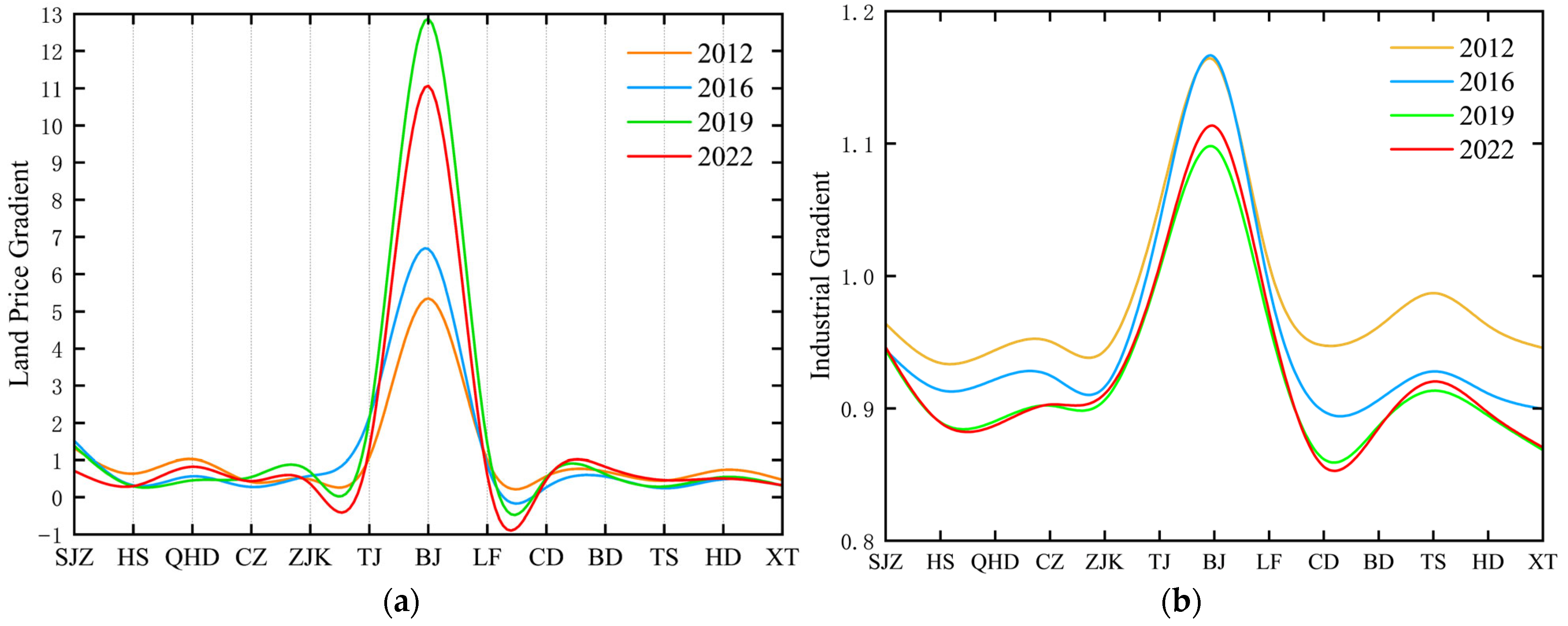
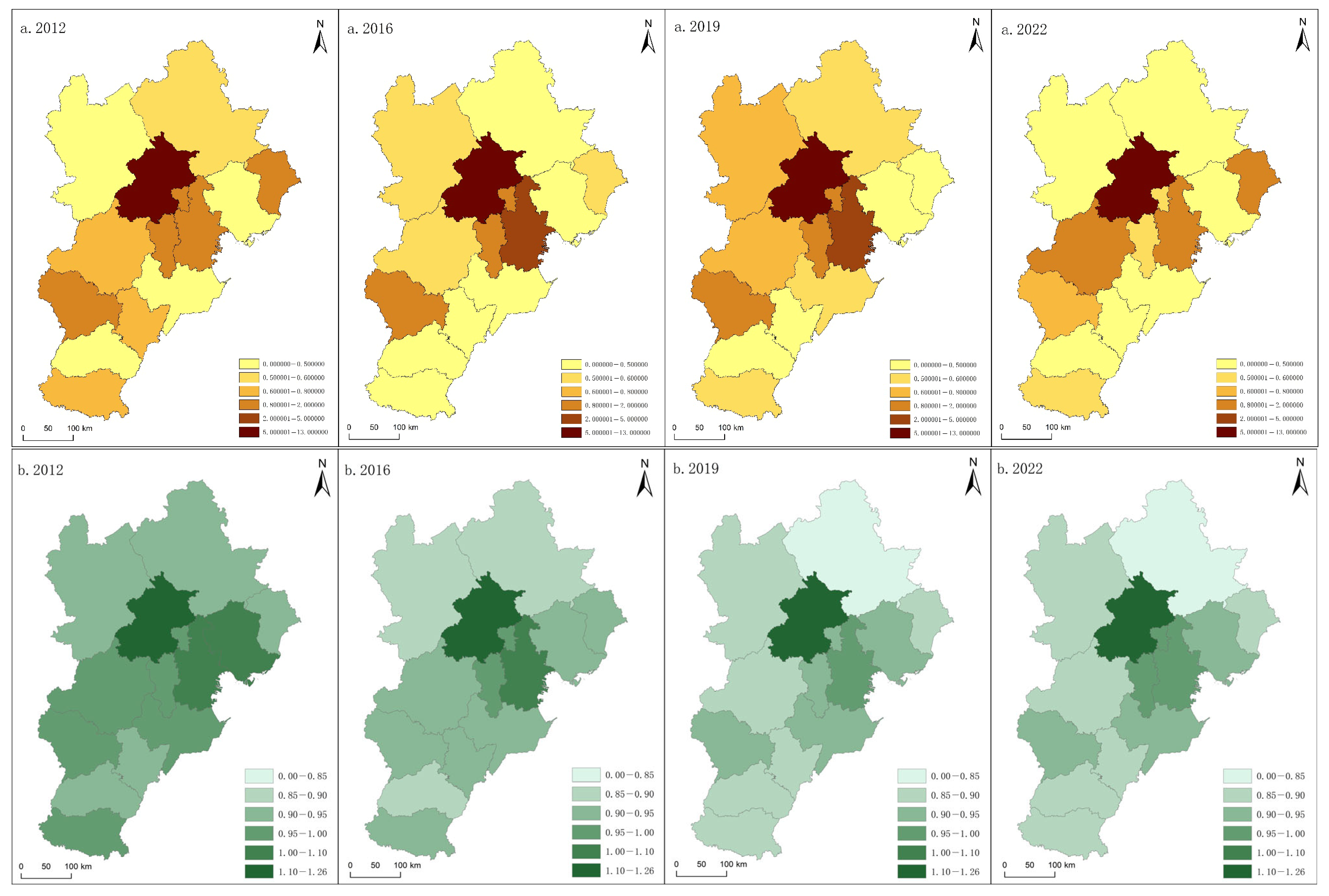
From a temporal perspective, land capital accumulation across cities in the BTHUA exhibited a dynamic pattern of concentration toward core cities such as Beijing and Tian-jin during 2012 to 2019. The disparity in land price gradients among other cities gradually narrowed, reflecting spatial imbalance in regional land price distribution—a pattern that began to ease after 2019 (Figure 2a). Specifically, Beijing’s land price gradient rose steadily from 2012 to 2019, with a slight decline observed thereafter. Both the gradient level and growth rate remained significantly higher than those of other cities in the region, placing Beijing securely in the top tier. Tianjin and Shijiazhuang, as sub-core cities, reached peak land price gradients around 2016, followed by a continuous decline, placing them in the region’s second tier. Langfang, Zhangjiakou, and Cangzhou showed an up-ward-then-downward trend in land price gradients in around 2019, whereas Qinhuangdao, Tangshan, and Baoding exhibited the opposite trend. The land price gradient range of Handan, Hengshui, Chengde, and Xingtai declined from [0.4, 1] to [0.3, 0.8] in 2012 to 2022.

During the study period, the industrial gradient of the BTHUA exhibited a typical “increasing-then-decreasing” pattern. However, the disparity in industrial gradient levels among cities narrowed, and the overall “slope” flattened gradually (Figure 2b). Specifically, Beijing maintained the highest industrial gradient in the urban agglomeration over the long term, showing a temporal trend of an initial decline followed by a rebound. Overall, its gradient decreased by 4.8%, reflecting industrial restructuring under the context of “downsized development” in large cities. The industrial gradients of Tianjin and Shijiazhuang peaked in 2016 and have since exhibited a steady downward trend, with cumulative declines of 4.69% and 1.84%, respectively. The trends observed in these three major cities suggest a gradual convergence in industrial structure between core and sub-core cities within the BTHUA. Among other cities in Hebei Province, traditional industrial and resource-based cities such as Cangzhou, Qinhuangdao, and Chengde experienced a year-by-year decline in industrial gradient indices. In contrast, cities adjacent to regional cores—such as Baoding and Langfang—exhibited decreases-then-increases industrial gradients.

Using a spatial contiguity weight matrix, we first apply the Global Moran’s I to test for spatial autocorrelation, and then employ the Local Moran’s I to analyze the spatial distribution characteristics of the land price and industrial gradients across cities in the BTHUA. The Global Moran’s I indices for both land price and industrial gradients fall within the range of [−1, 0], and the p-values for 2012 and 2022 exceed 0.1, indicating no significant spatial dependence. Nevertheless, the Local Moran’s I scatterplots still yield meaningful descriptive insights into spatial distribution patterns. For land price gradients, Tianjin, Qinhuangdao, and Langfang consistently fall within the H–H quadrant; Beijing and Shijiazhuang remain in the H–L quadrant; Hengshui and Cangzhou persist in the L–H quad-rant; and Chengde is consistently located in the L–L quadrant. Meanwhile, the clustering patterns of other cities vary substantially. This suggests that the local spatial structure of land price gradients in the BTHUA exhibits three dominant features: (i) a monocentric high-value cluster centered on Beijing; (ii) a sub-high-value ring represented by Tianjin and Langfang; and (iii) low-value zones located in the northern mountainous and south-eastern peripheral regions, represented by Chengde and Cangzhou (Figure 3a). For industrial gradients, both Beijing and Tianjin shift from the H–H to the H–L quadrant; Zhangjiakou and Shijiazhuang consistently occupy the H–L quadrant; Baoding, Handan, and Xingtai remain in the L–H quadrant; and Tangshan and Chengde are persistently located in the L–L quadrant. This indicates that the local spatial structure of industrial gradients in the BTHUA is characterized by three main patterns: (i) an intensifying trend of industrial agglomeration in core cities such as Beijing, Tianjin, and Shijiazhuang; (ii) a low-value industrial gradient belt formed by peripheral cities such as Handan and Xingtai; and (iii) traditional industrial and resource-based cities such as Tangshan and Chengde also embedded within the low-value belt (Figure 3b).

From a spatial perspective, in 2012, the BTHUA exhibited a spatial distribution pattern characterized by a high-value concentration of land price and industrial gradients in a single core, and dispersed low values across peripheral cities. Beijing had significantly higher land prices and a significantly higher position in the industrial hierarchy than all the other cities, serving as the sole core of the BTHUA. Although Tianjin’s land price and industrial levels were higher than those of the surrounding cities, the gap with Beijing remained substantial. Most other cities had relatively low land price and industrial gradient values, indicating a highly unbalanced spatial structure within the region. From 2012 to 2019, the spatial distribution of land price and industrial gradients in the BTHUA began evolving toward a multi-centered “point-axis” structure. Beijing and Tianjin emerged as dominant regional growth poles, with significantly higher gradient values than the other cities, forming a strong “dual-core” system. As the capital of Hebei Province, Shijiazhuang ranked highest in the province in terms of both land price and industrial gradients, serving as another key support point in the BTHUA. Among other peripheral cities, those closer to regional cores experienced faster growth in land and industrial gradients, enhancing the overall support capacity of the emerging “point-axis” urban system within the agglomeration. Overall, during this period, the BTHUA exhibited a spatial structure of “one core, one sub-core, and gradient diffusion.” However, the inter-city gap in gradient values widened, with visible segmentation between tiers. By 2022, the land price gradients in northern and southeastern cities of BTHUA had generally declined. A multi-nodal urban system centered on Beijing, Tianjin, and Shijiazhuang—along with ad-jacent peripheral cities—played an increasingly prominent supporting role in the regional structure. The BTHUA ultimately evolved a relatively balanced, polycentric, and concentric-ring spatial structure.

Overall, from 2012 to 2022, cities within the BTHUA exhibited a distinct core–periphery gradient pattern and a multi-centered, concentric spatial structure in both land price and industrial gradients. In terms of land price gradients, the highest value was observed in Beijing, while Tianjin and Shijiazhuang belonged to the second tier. The land prices in other cities gradually declined with an increase distance from the central cities, forming a spatial gradient pattern of “one core, multiple nodes, and multiple concentric tiers” (Figure 4a). Regarding industrial gradients, Beijing maintained a significantly higher level than the surrounding cities. Tianjin and Shijiazhuang served as major manufacturing hubs and secondary service clusters, with stable positions in the second tier of the industrial gradient. Together, these three cities formed the core support points for industrial development across the urban agglomeration. Langfang, Cangzhou, and Bao-ding—serving as intermediary cities—had lower industrial gradients than the central cities but higher gradients than the cities on the periphery. The combination of regional central cities and adjacent node cities formed a multi-centered, concentric industrial spatial structure within the region (Figure 4b).

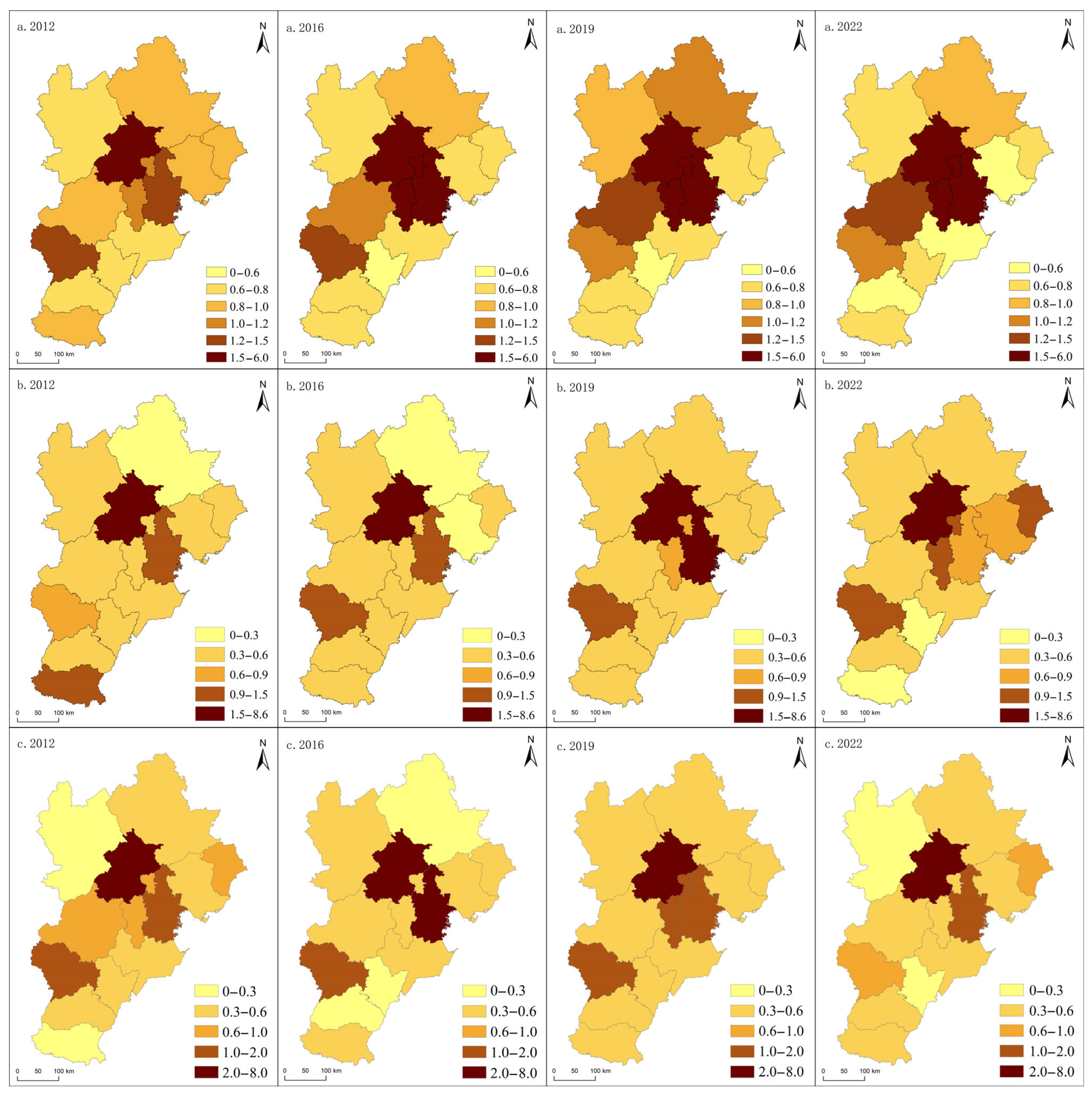
Based on land use categories, the land price gradients are divided into industrial, commercial service, and residential types for analysis. For industrial land price gradients, Beijing and Tianjin—acting as the dual engines of regional development—maintain high levels and generate spatial spillovers along the Beijing–Tianjin and Beijing–Baoding–Shijiazhuang corridors, forming a concentric spatial distribution pattern (Figure 5a). For commercial-service land price gradients, Beijing consistently holds the highest values, producing spillover effects along the Beijing–Tianjin corridor. As regional sub-centers, Tianjin and Shijiazhuang maintain relatively high values, while Tangshan has shown a steady upward trend since 2016. In contrast, other peripheral cities remain in low-value zones (Figure 5b). For residential land price gradients, the BTHUA exhibits a “single-core plus secondary-core” pattern, with Beijing and Tianjin functioning as dual high-value nodes. Before 2019, spillover effects extended along the Beijing–Tianjin and Beijing–Baoding–Shijiazhuang corridors, generating concentric high-value belts. After 2019, however, the residential land price gradients in peripheral cities broadly declined, exacerbating spatial imbalances (Figure 5c). Among the reporting years, in 2019, the number of residential land transactions totaled 9 in Beijing and 20 in Qinhuangdao, while the number of commercial-service land transactions in Qinhuangdao in 2022 totaled 24. These three cases represent small samples from a statistical perspective and differ substantially from other panel data observations. Accordingly, potential biases arising from these small sample sizes cannot be excluded, and the corresponding results should be interpreted with caution.

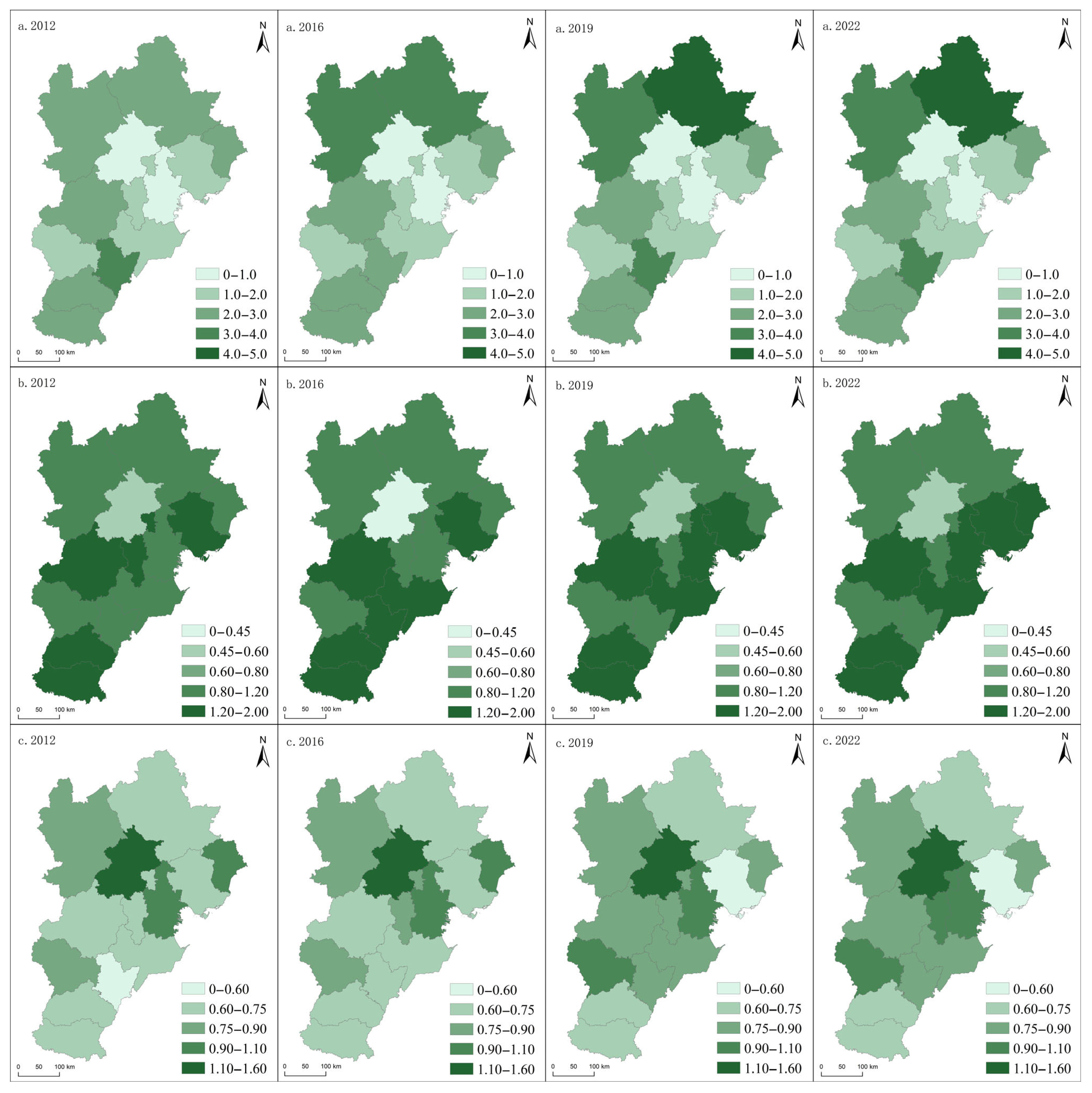
Based on the three-sector classification, we analyze the gradients of the primary, secondary, and tertiary industries separately. For the primary industry, the BTHUA exhibits an overall spatial pattern characterized by low values in the core and high values on the periphery. Specifically, the resource-rich Southern Hebei Plain and the northern mountainous areas jointly constitute a high-value belt in the primary industry. By contrast, due to industrial upgrading and rising factor costs, core and sub-core cities such as Beijing and Tianjin have long maintained low gradient values in the primary industry (Figure 6a). For the secondary industry, the BTHUA displays a ring-shaped high-value belt surrounding Beijing. Beijing itself remains at a medium-to-low level, whereas nearby cities such as Tianjin, Tangshan, and Baoding, along with southern peripheral cities, maintain persistently high gradient values. This pattern has gradually evolved into two advantageous belts of secondary industry: one along the eastern coastal port areas and the other in the southern plain (Figure 6b). Regarding the tertiary industry, the BTHUA reveals a spatial structure consisting of “one core, two sub-cores, and a concentric decline.” The northeastern and southern peripheral cities consistently remain in low-value zones (Figure 6c).

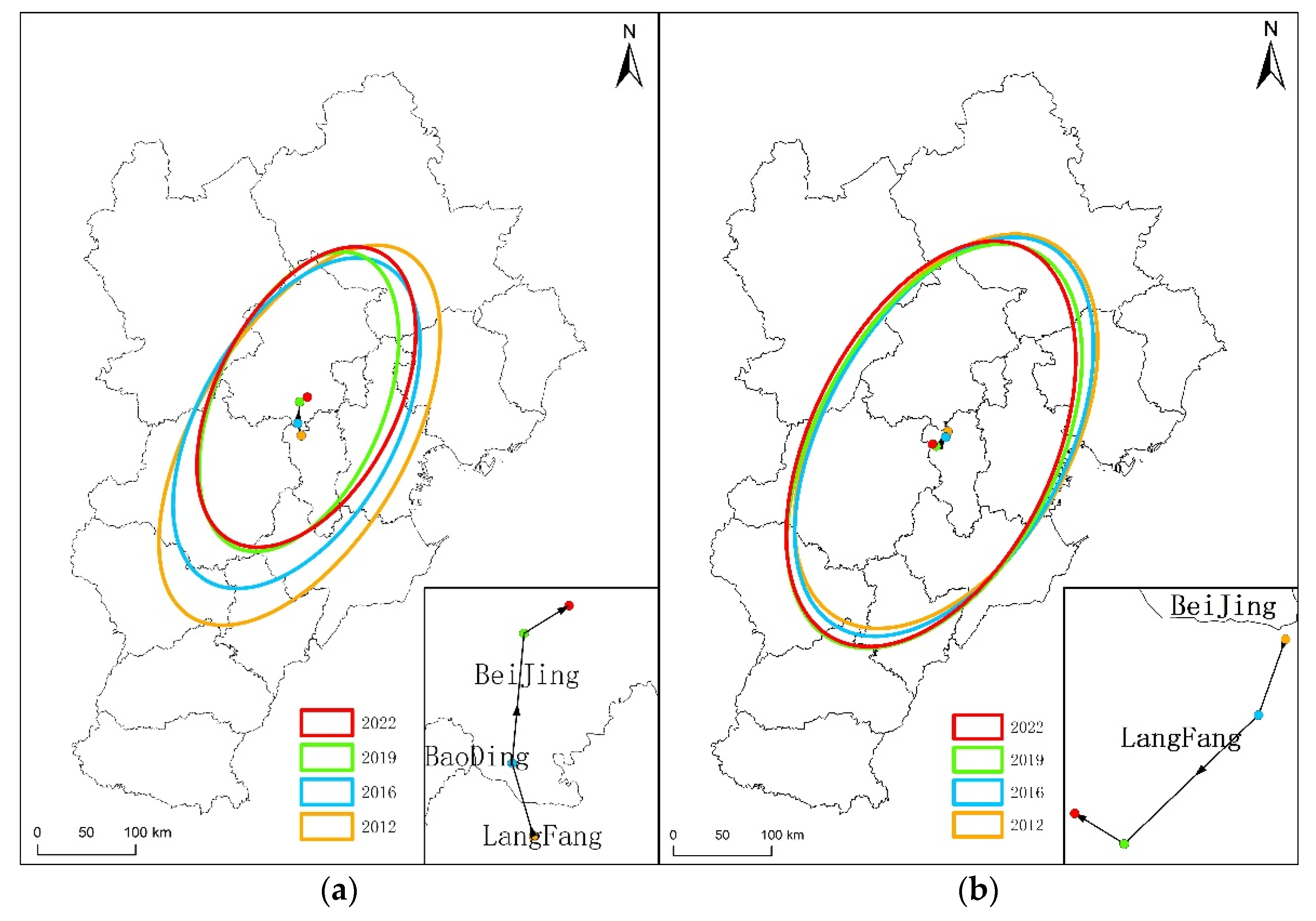
The standard deviation ellipse method was further applied to analyze the degree and direction of spatial concentration for land price and industrial gradients in the BTHUA. Regarding land price gradients, the ellipse area shrank by 39.61% between 2012 and 2019, followed by a 15.25% increase by 2022, indicating a phase of strong concentration in core cities followed by moderate diffusion. In terms of spatial orientation, the ellipse centroid continuously shifted toward Beijing from 2012 to 2022, indicating Beijing’s growing dominance and siphoning effect on regional land value (Figure 7a). For industrial gradients, the ellipse area in the BTHUA showed a mild decline followed by a rebound between 2012 and 2022 (Figure 7b), indicating that the region’s industrial agglomeration level remained relatively stable during the study period, with only gradual structural adjustments driven by the relocation of non-core functions from Beijing, functional reception by neigh-boring cities, and the emergence of new growth poles. As a result, the regional industrial center gradually shifted southward.

5.2. Spatio-Temporal Characteristics of the Multidimensional Coupling Between Land Price Gradients and Industrial Gradients

5.2.1. Spatio-Temporal Characteristics of Static Coupling

The static coupling degree between land price gradients and industrial gradients reflects the degree of coordination between land factor allocation and the spatial layout of industries within the urban agglomeration. A high level of coupling between the two indicates that the region has largely achieved spatial equilibrium between land and industry, where industrial development and land value reinforce each other in a virtuous cycle. In contrast, a low degree of coupling suggests a spatial mismatch between land resource allocation and industrial distribution. On one hand, this could manifest as inflated land prices unsupported by industrial fundamentals—a sign of a potential real estate bubble. On the other hand, it could reflect excessive land supply leading to depressed land values. Both scenarios point to uncoordinated regional development.

From a time-series perspective, the degree of static coupling between land price gradients and industrial gradients in most cities in the BTHUA showed a declining trend during the 2012–2019 period. Notably, Tangshan, Qinhuangdao and Hengshui experienced significant decreases. Between 2019 and 2022, cities such as Beijing, Tangshan, Baoding, Qinhuangdao, and Xingtai continued to see improvements in their static coupling levels, whereas most other cities experienced declines. The magnitude of change was particularly notable in Langfang, Hengshui, and Zhangjiakou (Figure 8). Moreover, the radar chart below reveals that from 2012 to 2019, core and sub-core cities such as Beijing, Tianjin, and Shijiazhuang, together with nearby cities such as Langfang, maintained high or moderately high levels of static coupling. After 2019, however, only Beijing and Tianjin sustained relatively high levels, whereas the static coupling levels of other cities declined. the curves in 2012, 2016, and 2019 appear relatively irregular, while the 2022 curve is notably smoother, indicating pronounced disparities in static coupling among cities in 2012, reflecting the significant spatial imbalance at that time. Although gradual further deteriorations were observed in the following years, signs of spatial improvement after 2019.

Using a spatial contiguity weight matrix, we apply the Global Moran’s I and Local Moran’s I to test the spatial autocorrelation of the static coupling between the land price and industrial gradients and analyze their spatial distribution patterns. The Global Moran’s I indices for the static coupling between the land price and industrial gradients fall within the range [0, 1], with p-values of 0.049 in 2012 and 0.078 in 2022, both below 0.1, indicating significant spatial dependence. The Local Moran’s I scatterplots further show that Beijing, Langfang, and Baoding consistently fall within the H–H quadrant; Shijiazhuang remains in the H–L quadrant; Tangshan, Zhangjiakou, Cangzhou, and Chengde persist in the L–H quadrant; and Xingtai and Handan remain in the L–L quadrant. Meanwhile, Tianjin and Qinhuangdao exhibit notable shifts in their spatial positions. These findings highlight several key features of the local spatial structure of static coupling in the BTHUA: (i) from 2012 to 2022, the spatial correlation of static coupling strengthened; (ii) a high-value belt centered on Beijing demonstrates spillover effects along the Beijing–Tianjin corridor; (iii) Shijiazhuang, as a regional sub-core, maintains relatively high static coupling, although its surrounding cities remain at low levels; and (iv) most peripheral cities display consistently low static coupling levels. Overall, the BTHUA contains a highly static-coupled corridor supported by the core and sub-core cities of Beijing, Tianjin, and Shijiazhuang, reflecting a pronounced polarization effect in the coordinated development of land prices and industries (Figure 9).

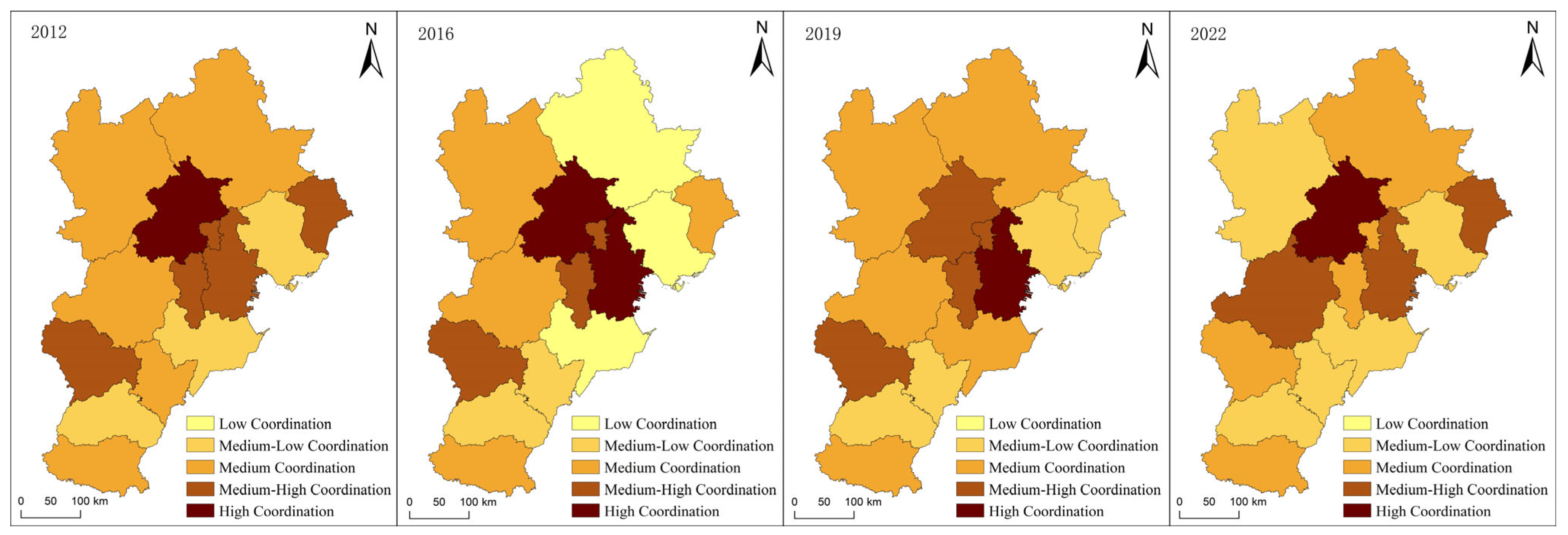
From a spatial perspective, the static coupling between land price gradients and industrial gradients in the BTHUA first increased and then declined over the study period. Cities with medium-high or higher levels of coupling exhibited a pronounced “core–periphery” pattern and a ring-shaped spatial distribution. Specifically, in 2012, the static coupling between land price and industrial gradients in the BTHUA formed a medium- to high-level distribution belt, with Beijing as the core and Tianjin and Shijiazhuang serving as supporting centers (Figure 10). Among the cities in this region, Beijing recorded coupling values of between 0.9 and 1.0, while Shijiazhuang fell within the 0.8–0.9 range. The coupling values for Tianjin, Langfang, and Qinhuangdao ranged from 0.7 to 0.8. These five cities were categorized as well-coupled, whereas the others remained at moderate or lower coupling levels. In 2016, the coupling levels still followed a “higher in the west, lower in the east” trend. The coupling values of core, sub-core, and eastern cities show an upward trend, with the supporting roles of regional core and sub-core cities—such as Beijing, Tianjin, and Shijiazhuang—becoming increasingly pronounced. By 2019, the levels of static coupling most cities further improved, with significantly reduced disparities be-tween them. In 2022, regional disparities in static coupling levels within the BTHUA widened once more, forming a concentric medium- to high-level coupling belt centered on Beijing and Tianjin.

Based on the relative magnitudes of land price and industrial gradients, cities can be categorized into four types: high coupling with a land gradient exceeding the industrial gradient (High-Land > Industry), high coupling with an industrial gradient exceeding the land gradient (High-Industry > Land), low coupling with a land gradient exceeding the industrial gradient (Low-Land > Industry), and low coupling with an industrial gradient exceeding the land gradient (Low-Industry > Land). We found that in cities with high levels of static coupling—such as Beijing, Tianjin, Shijiazhuang, and Langfang—the land price gradient exceeded the industrial gradient from 2012 to 2019, whereas after 2019 the industrial gradient gradually surpassed the land price gradient. In contrast, other cities exhibited low levels of static coupling, suffered negative impacts from persistently high land or industrial gradients, which hindered improvements in their coupling levels (Figure 11). An industrial gradient is relatively high, it may reflect land cost depressions that favor industrial diffusion and relocation within the urban agglomeration. On the other hand, it may lead to low land use efficiency and market distortion. Regional sub-centers such as Tianjin and Shijiazhuang have attracted mid- and low-end industries that have relocated from Beijing by offering relatively low land prices, thereby advancing industrial division and promoting spatial balance within the urban agglomeration. However, long-term reliance on “land cost depressions” risks giving rise to excessive siphoning effects on peripheral cities, trapping them in a “low land price–low industry” cycle of in-efficiency. Distorted land prices may further inhibit industrial upgrading in sub-center cities. Overall, the relative magnitudes of land and industrial gradients can generate both positive effects—such as mutually reinforcing spiral growth—and negative effects—such as resource misallocation and reduced spatial efficiency. The positive impacts are most pronounced in core cities like Beijing, Tianjin, and Shijiazhuang, while negative effects are more evident in smaller peripheral cities. In most cities, the industrial gradient exceeds the land price gradient.

5.2.2. Spatio-Temporal Characteristics of Dynamic Coupling

Next, using a spatial contiguity weight matrix, we again apply the Global Moran’s I and Local Moran’s I to test the spatial autocorrelation of the dynamic coupling between the land price and industrial gradients and analyze their spatial distribution characteristics. The Global Moran’s I indices for the dynamic coupling between the land price and industrial gradients fall within the range [−1, 0], with p-values of 0.047 in 2012 and 0.040 in 2022, both below 0.1, indicating significant spatial dependence. The dynamic coupling index is defined as a negative indicator. The Local Moran’s I scatterplots further show that Chengde consistently falls in the H–L quadrant; Beijing, Tangshan, Qinhuangdao, and Zhangjiakou re-main in the L–H quadrant; and Hengshui and Cangzhou persist in the L–L quadrant. Meanwhile, whereas other cities exhibit notable shifts in their clustering patterns. These findings indicate that the local spatial structure of dynamic coupling between the land price and industrial gradients in the BTHUA exhibits the following features: (i) from 2012 to 2022, the spatial correlation of dynamic coupling followed a convergent trend; (ii) the pattern combined dispersed distribution with axial diffusion. Two polarized belts emerge—one centered on Beijing and the other in Eastern Hebei—alongside a relatively balanced belt in southeastern Hebei represented by Hengshui and Cangzhou (Figure 12).

The degree of dynamic coupling between land price gradients and industrial gradients reflects the degree of coordination between land price growth and industrial structure adjustment within the urban agglomeration (Figure 13). Over the 2012–2022 period, the dynamic coupling levels in most cities in the BTHUA exhibited an overall inverted-U trend—rising first and then declining. From 2012 to 2016, the dynamic coupling degrees increased in ten cities including Tianjin, Langfang, Cangzhou, while they declined in Beijing, Baoding, Zhangjiakou. From 2016 to 2019, the dynamic coupling levels of Beijing, Xingtai, Baoding, and Qinhuangdao improved significantly, whereas those of six cities—including Tianjin, Tangshan, and Zhangjiakou—declined. In the remaining cities, changes in dynamic coupling levels were negligible. Between 2019 and 2022, Tianjin, Shijiazhuang, and Tangshan exhibited an upward trend in dynamic coupling. The dynamic coupling levels of seven cities, including Beijing, Chengde, Baoding, and Qinhuangdao, all show a downward trend.

In terms of spatial distribution, the dynamic coupling across cities in the BTHUA in 2012 displayed an overall “high in the west, low in the east” pattern, with five cities—Beijing, Zhangjiakou, Baoding, Shijiazhuang, and Hengshui—recording medium-high or higher levels of dynamic coupling. By 2016, cities along the southeastern corridor of the region experienced significant increases in dynamic coupling. Notably, Qinhuangdao, Hengshui, Tangshan, and Cangzhou moved up in the coupling classification, suggesting a spatial shift in the focus of coordination between land prices and industrial development—from west to east. In 2019, the dynamic coupling distribution of the BTHUA exhibited a highly coupled zone centered on Beijing and its surrounding cities, diffusing outward along the north–south axis in a progressively declining manner and forming a concentric spatial pattern. In 2022, the distribution of the dynamic coupling between land price and industrial gradients exhibited a belt-shaped pattern along the Beijing–Tianjin and Beijing–Baoding–Shijiazhuang corridors.

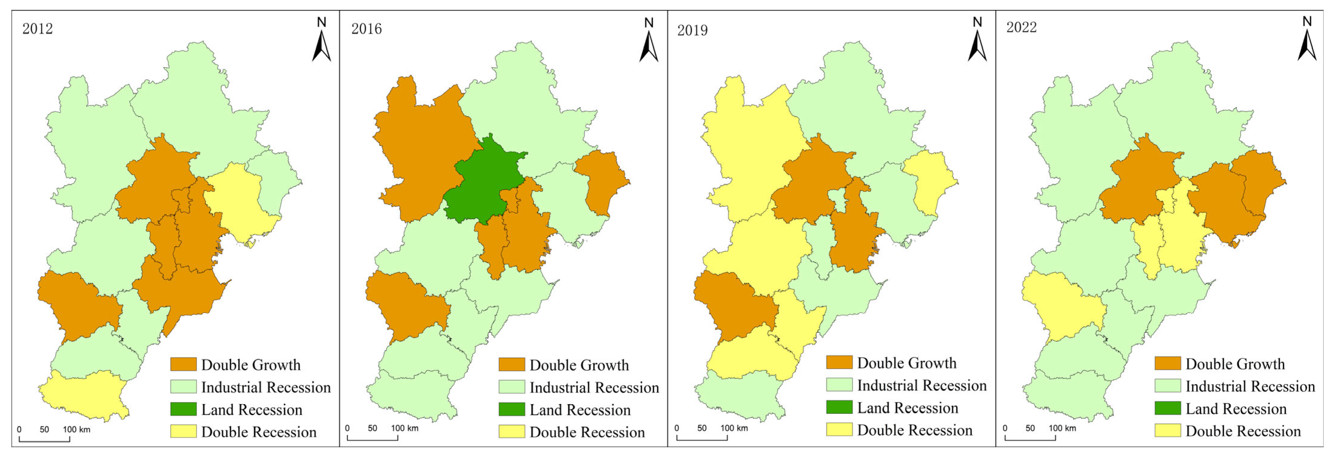
Based on the direction of change in land price and industrial gradients, cities can be classified into four types: industrial recession (a declining industrial gradient with a rising land price gradient), land recession (a declining land price gradient with a rising industrial gradient), double recession (both gradients declining), and double growth (both gradients increasing). The results of our analysis reveal that all the cities experienced a shift in development type, shedding light on the evolving relationship between land allocation and industrial development (Figure 14). From an evolutionary perspective, in 2012 core and sub-core cities such as Beijing and Tianjin were undergoing urban expansion and industrial upgrading, with both land price and industrial gradients showing syn-chromous growth. By contrast, peripheral cities such as Chengde, Zhangjiakou, and Xing-tai experienced an asymmetric trajectory—rising land price gradients but declining industrial gradients—whereas Tangshan and Handan exhibited simultaneous declines in both. In 2016, Beijing recorded a decline in its land price gradient, whereas most other cities continued to show rising gradients. At the same time, the industrial gradients of five cities—including Tianjin, Shijiazhuang, and Langfang—increased, whereas those of the remaining cities declined. In 2019, Beijing, Tianjin, and Shijiazhuang, as regional core and sub-core cities, sustained synchronous growth in both land price and industrial gradients. However, the number of cities experiencing simultaneous declines in both gradients in-creased. The industrial gradients of Tangshan, Chengde, Cangzhou, Handan, and Lang-fang turned negative, signaling the initial deterioration of land price–industry coordination in the BTHUA. In 2022, Tianjin, Shijiazhuang, and Langfang experienced simultaneous declines in both land price and industrial gradients, whereas Beijing, Tangshan, and Qinhuangdao registered synchronous growth in both. The remaining cities continued to exhibit negative growth in their industrial gradients. Overall, from 2012 to 2022, most BTH cities experienced synchronous gradient changes. Cities in double-recession trajectories were more likely to suffer prolonged industrial decline. Cities with higher dynamic coupling levels—such as Beijing, Qinhuangdao, and Langfang—were more likely to maintain parallel growth in both gradients. Additionally, cities surrounding Beijing were more prone to either land or industrial gradient recession. Both Tianjin and Shijiazhuang, as secondary regional centers, experienced land price gradient declines.

5.2.3. Spatio-Temporal Characteristics of Spatial Matching Degree

Next, using a spatial contiguity weight matrix, we apply the Global Moran’s I and Local Moran’s I to test the spatial autocorrelation of the spatial matching between the land price and industrial gradients and analyze their spatial distribution characteristics. The Global Moran’s I indices for spatial matching between the land price and industrial gradients fall within the range [−1, 0]. The p-value for 2012 is above 0.1, whereas the p-value (p = 0.047) for 2022 is below 0.1, indicating significant spatial dependence in 2022. The spatial matching index is defined as a negative indicator. The Local Moran’s I scatterplots further show that Beijing, Tangshan, Qinhuangdao, and Zhangjiakou fall within the L–H quadrant; Cangzhou and Hengshui are located in the L–L quadrant; and Chengde lies in the H–L quadrant. Meanwhile, the spatial distribution patterns of the other cities have shifted. These results indicate that the local spatial structure of spatial matching in the BTHUA has several notable features: (i) spatial matching radiates from the Beijing core toward Tianjin and Tangshan, forming highly matched “islands” anchored by these three cities; (ii) by 2022, cities in Southern Hebei, represented by Shijiazhuang, and those in Northwestern Hebei, represented by Zhangjiakou, formed a relatively balanced medium-level spatial matching belt (Figure 15).

The degree of spatial matching between land price and industrial gradients reflects the spatial equilibrium level within the urban agglomeration (Figure 16). In terms of temporal evolution, from 2012 to 2016, the degree of spatial matching in the BTHUA exhibited a divergent trend—rising in areas surrounding Beijing while declining in peripheral cities. The degree of spatial matching increased in the core cities of Beijing and Tianjin, as well as in nearby cities such as Baoding, Langfang, and Zhangjiakou. In contrast, cities in the northeastern and southern parts of the region experienced a decline. Between 2016 and 2019, under the coordinated development strategy of the region, most cities showed improvements in spatial matching. Notably, Zhangjiakou, Handan, Langfang, and Xingtai witnessed significant increases, while only Baoding saw a marked decline. From 2019 to 2022, spatial matching in the region declined again. Except for Qinhuangdao and Tangshan, all the other 11 cities experienced decreases, with Langfang and Handan seeing particularly sharp declines. Overall, from 2012 to 2022, the spatial matching between land price and industrial gradients in the BTHUA followed a time-varying trajectory of “initial increase, subsequent decline, renewed rise, and eventual decrease.”

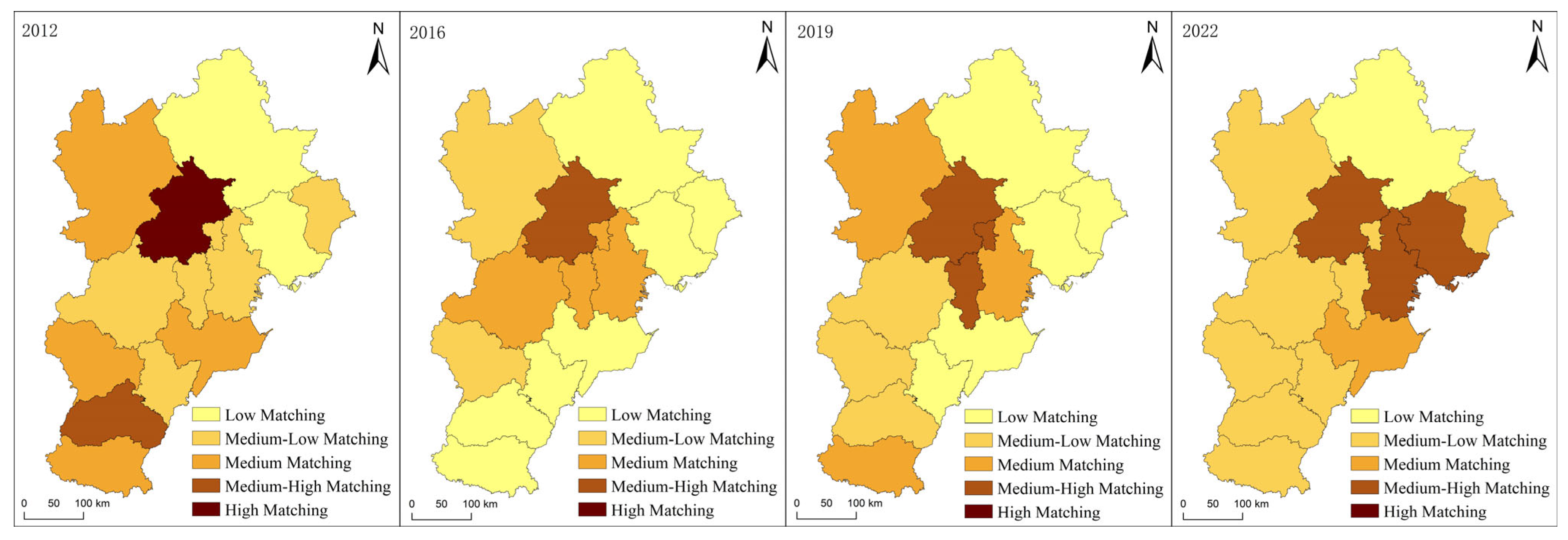
Spatially, in 2012, the medium- and high-level spatial matching between land price and industrial gradients in the BTHUA displayed a dispersed distribution, with Beijing and southern cities such as Shijiazhuang forming medium- to high-matching areas. In 2016, the spatial matching pattern demonstrated a trend of contraction toward core cities and their surrounding areas, primarily reflected in a medium- to high-level matching zone formed by Beijing, Tianjin, and their southern neighboring cities. In 2019, overall spatial matching improved in the BTHUA, with high-matching zones forming a “point-axis” pattern centered on Beijing and Tianjin and extending toward adjacent peripheral cities. While the disparities between most cities narrowed, the overall regional gap widened, indicating a Matthew effect in land-industry spatial balance. In 2022, the spatial matching between land price and industrial gradients declined in most cities of the BTHUA; nevertheless, the overall spatial matching remained low but relatively balanced. Medium- to high-level matching areas exhibited a corridor-shaped spatial pattern centered on Beijing and Tianjin.

Based on the relative strengths of the land price and industrial gradients as well as their spatial matching levels, cities can be categorized into four types: Land-Dominant High Coordination (LHC), Land-Dominant Low Coordination (LLC), Industry-Dominant High Coordination (IHC), and Industry-Dominant Low Coordination (ILC). As shown in Figure 17, the majority of the cities fall into the ILC category. These are typically traditional manufacturing cities, where local governments tend to expand the supply of industrial land in order to lower land costs for businesses, aiming to attract investment or maintain a competitive edge in manufacturing. The resulting oversupply of land and its inefficient use are major contributors to spatial resource mismatches. Moreover, owing to the limited capacity of the secondary sector, the low land price model constrains industrial upgrading, trapping regions in a spatially unbalanced development cycle of “low land prices–low matching.” Cities of the LLC type are mainly located near sub-core cities. Their land prices are positively influenced by the externalities of nearby high-price urban centers, while their industries are siphoned away by these cores, resulting in land-industry spatial mis-match. Among regions with high land–industry coordination, most are Industry -dominant cities—typically core or peri-core cities. These areas feature a high proportion of tertiary industries and stronger population and economic agglomeration. Because land prices are more sensitive to market demand, the land price gradient tends to respond more quickly than the industrial gradient under external shocks.

5.2.4. Robustness Check

To account for interannual fluctuations and extreme-value disturbances in the three coupling indicators—SCI, DCI, and SME—this study applies a three-year moving average to smooth the series, using a trailing window to adjust the endpoints. Compared with the original specification, the mean square error of each indicator is reduced under the three-year moving average approach (

Table 5. Mean Squared Errors of SCI, DCI, and SME.

City	MSE-SCI	MSE-DCI	MSE-SME
Beijing	0.00077	0.015512	0.138425
Tianjin	0.002169	0.013683	0.038244
Shijiazhuang	0.004751	0.017911	0.044073
Tangshan	0.01254	0.111707	0.068894
Qinhuangdao	0.004986	0.000756	0.059584
Handan	0.004094	0.002736	0.062661
Xingtai	0.002941	0.073021	0.066068
Baoding	0.007213	0.066271	0.065606
Zhangjiakou	0.009011	0.001694	0.062054
Chengde	0.002657	0.3928	0.065463
Cangzhou	0.016792	0.001405	0.068942
Langfang	0.005884	5.702432	0.055701
Hengshui	0.00926	0.000758	0.067463

). The regional average trends and spatial patterns remain consistent, and the spatial gradients exhibit no directional change, with only mi-nor fluctuations near critical thresholds observed in a few peripheral cities. Overall, the conclusions of this study are robust to the smoothing adjustment. The smoothed results are employed solely for robustness testing, while the baseline findings continue to depend on the original measurements.

6. Influencing Factors and Nonlinear Mechanisms of the Coupling Relationship

6.1. Variable Selection

This study explores the multidimensional coupling characteristics between land price gradients and industrial gradients across cities in BTHUA from three perspectives: development level, rate of change, and spatial matching. It further treats static coupling degree (SCI), dynamic coupling degree (DCI), and spatial matching efficiency (SME) as dependent variables, and investigates the key influencing factors and their nonlinear mechanisms.

Drawing on the literature on urban land price determinants [67,68] and regional industrial development drivers [69,70], we selected 15 variables from five key dimensions—geographical conditions, locational advantages, city size, public services and infrastructure, and economic development—as explanatory variables (

Table 6. Selection of Indicators and Variable Descriptions.

Influencing Factors	Indicator Name	Variable Symbol	Variable Description
Geographical Conditions	Average elevation	ln(ele)	Calculated as the mean elevation of each city based on DEM data
	Terrain slope	slope	Calculated as the mean terrain slope within each city’s administrative boundary using DEM data
	Urban area	ln(area)	Total administrative area of each city
Locational Conditions	Distance to coastline	ln(disc)	Straight-line distance from each city center to the nearest coastline
	Distance to core city	ln(dis)	Straight-line distance from each city to the core city
Urban Scale	Economic scale	ln (GDP)	Regional GDP
	Population scale	ln(pop)	Year-end resident population of each city
	Administrative level	adm	Assigned values from 1 to 4 by administrative hierarchy
Public Services and Infrastructure	Basic education	edu	Number of primary and secondary school students per 10,000 population
	Basic healthcare	hos	Number of hospital beds per 10,000 population
	Urban green coverage	green	Green coverage ratio in built-up areas
Economic Development	Average wage	ln(wage)	Average wage of employees in non-private urban units
	Fiscal expenditure	Ln (Fisc)	Total local general public budget expenditure
	Financial development	ln(finan)	Year-end total deposits and loans of financial institutions
	Number of patents granted	ln(pat)	Total number of patents granted annually

). The descriptive statistics are shown in

Table 7. Descriptive statistics.

Variable	Obs	Mean	Std	Min	Max	Variable	Obs	Mean	Std	Min	Max
SCI	143	0.556	0.227	0.009	0.999	Lnpop	143	6.581	0.557	5.711	7.634
DCI	143	0.429	1.491	0.001	13.817	Adm	143	1.538	0.993	1	4
SME	143	0.869	0.148	0.036	0.999	Edu	143	0.126	0.033	0.059	0.197
Lnele	143	4.789	1.539	2.397	7.134	Hos	143	44.329	6.553	27.323	59.912
Slope	143	7.696	4.420	2.180	16.271	Green	143	0.424	0.036	0.349	0.498
Lnarea	143	9.580	0.518	8.761	10.590	Lnwage	143	7.256	3.123	3.295	21.508
Lndisc	143	4.947	0.755	3.641	5.846	Lnfisc	143	15.711	0.913	14.291	18.129
Lndis	143	4.828	1.486	0.010	6.006	Lnfinan	143	18.566	1.132	16.941	21.848
lngdp	143	17.398	0.929	16.129	19.846	lnpat	143	8.494	1.489	5.313	12.220

.

6.2. Factor Analysis and Nonlinear Mechanisms

Based on the feature importance rankings derived from the GBDT model, the top nine most important indicators were extracted separately for each of the three dependent variables. Overall, “second nature” factors exerted a stronger influence on the multidimensional coupling degrees than “first nature” factors, as shown in

Table 8. Results of the GBDT.

SCI-Top9		DCI-Top9		SME-Top9
Variable	Influence	Variable	Influence	Variable	Influence
Lnwage	21.08%	Hos	33.51%	Lnfisc	39.40%
lnpop	17.24%	Lnwage	15.37%	Edu	16.59%
Lndisc	12.87%	lndis	12.69%	Lnpop	12.03%
Lnpat	8.18%	Green	9.89%	Lnfinan	10.54%
Lnarea	7.23%	Lngdp	9.13%	Hos	4.20%
Green	6.68%	Lnpat	7.78%	Lnpat	3.54%
Lndis	5.66%	Lnfisc	3.25%	Green	3.42%
Hos	4.97%	Edu	3.03%	Lngdp	3.11%
edu	4.33%	lnpop	2.99%	lnarea	3.03%

.

Among the influencing factors, economic development and the city size play the dominant roles in shaping the static coupling between land price gradients and industrial gradients. Geographic and locational conditions also exert significant impacts, while public services have a relatively limited effect. Further analysis of the partial dependence plots (PDPs) for the top nine explanatory variables, ranked by feature importance (Figure 18a), reveals several patterns. Firstly, the PDP curves for fiscal expenditure, financial development, pa-tent authorizations, and urban greening exhibit upward trends. Increases in fiscal expenditure enhance both the “hard power” of urban infrastructure and the “soft power” of social welfare, which raises the land value-added and attract high-value-added industries, thereby strengthening land–industry coupling. Greater financial development improves the capital allocation efficiency, and the profit-seeking behavior of capital facilitates the agglomeration of high-value-added industries. Under rapid urbanization and the fiscal reliance of local governments on land revenues, the capitalization of land is also promoted. Together, these processes reflect the coordinated interaction among land, capital, and industry in spatial agglomeration. Patent authorizations partly reflect a city’s innovation capacity. Knowledge and technology-intensive industries are more adaptable to high land prices and tend to cluster in core or sub-core cities with strong knowledge and technology spill-overs, thereby promoting higher gradient coupling. A high level of urban greening signals better urban quality, effectively increasing land rent premiums and enhancing the attractiveness of value-added industries. Moreover, investment in environmental governance raises land prices while simultaneously eliminating low-end, high-pollution, and energy-intensive industries. Secondly, the PDP curves for the urban population size, basic healthcare, and urban area show a “decline–increase” pattern. During rapid urbanization, land prices in small- and medium-sized cities rise rapidly in line with the economic cycle, but industrial development lags due to the siphon effect of core cities, creating spatial mismatch of “high land prices and low-end industries”. In large and mega-cities, land prices also rise rapidly, but faster and higher-quality industrial restructuring generates a virtuous cycle of “high factor prices and high industrial efficiency”. Weak healthcare systems indicate lower social welfare standards, reducing land value added and diminishing its attractiveness to firms and production factors. Conversely, strong healthcare systems attract high-quality labor and high-value-added industries, sustaining a high degree of coordination between land prices and the industrial structure. In smaller cities, limited land supply raises the land use costs for firms. In larger cities, continuous urban land expansion creates functionally differentiated, polycentric structures that attract diverse enterprises and, through combined market mechanisms and government regulation, generate land price gradients aligned with industrial gradients. Thirdly, the PDP curves for the distance from the core city and basic education exhibit a downward trend. A greater distance from the core city reduces transport accessibility and weakens spatial spillover effects. Consequently, the industrial structures of small and medium-sized cities on the inner peripheries of core areas are negatively affected, while land prices continue to rise under rapid urbanization, producing spatial mismatch consisting of “high land prices and low-level industries”. In China, the enrollment system linking household registration to school districts drives land prices upward through school district premiums and encourages the expansion of consumer-oriented services, but this provides limited stimulus for other industries. As a result, industrial upgrading progresses relatively slowly, and the static coupling between the land price and industrial gradients remains weak.

Economic development and public services are the primary drivers of the dynamic coupling between land price gradients and industrial gradients, whereas geographical conditions, locational attributes, and the city size play relatively limited roles. Further analysis based on the ranked importance of variables resulted in partial dependence plots (PDPs) of the top nine explanatory factors (Figure 19a), with several findings. Firstly, The PDP curves for basic healthcare, basic education, average wages, and patent authorizations exhibit down ward trends. Continuous improvements in healthcare and education strengthen urban human capital and foster the clustering of high-value-added industries. High-quality public services also raise land rent premiums, thereby enhancing the dynamic coupling between industrial and land price gradients. Rising average wages signal improvements in human capital and industrial upgrading, crowd out low-value-added industries, and accelerate structural transformation. Higher wages improve firms’ and residents’ adaptability to elevated land prices, but they also increase labor costs, pushing the industrial structure toward high-value-added activities. Higher wage levels further generate a population siphon effect from surrounding areas, raising the land demand and prices, and thereby amplifying the rates of change in both the industrial and land price gradients. Cities with high numbers of patent authorizations are typically regional centers with strong agglomerations of high-value-added industries. Their greater innovation capacity shortens the “technology diffusion–industrial restructuring–spatial reallocation” cycle, enabling industries to respond more rapidly to land price changes and thereby enhancing dynamic coupling. Secondly, the PDP curves for the urban economic scale, fiscal expenditure, and population size display upward trends. During urbanization, expansionary fiscal policies raise land prices by improving infrastructure and public services, whereas productivity gains and deeper specialization in industry typically require long-term operation and gradual up-grading. Moreover, incentivized by land-based fiscal revenues, local governments often prioritize land development and short-term performance projects such as municipal showcase initiatives. This exacerbates the tendency for land prices to change more quickly than the industrial structures, resulting in low dynamic coupling. Rapid population growth accelerates land capitalization. In China, land urbanization has generally outpaced population urbanization, causing land prices to rise more rapidly due to multiplier effects. Meanwhile, population concentration initially fuels consumer services and real estate rather than productive industries, whose slower adjustments lower dynamic coupling in such cities. Thirdly, the PDP curves for the distance from core cities and urban greening remain relatively stable. The distance to core cities shows little variation during the sample period, with insufficient temporal heterogeneity, producing a relatively flat impact on changes in land prices and the industrial structure. Improvements in environmental quality from urban greening affect industries heterogeneously. Moreover, because greening projects are often implemented simultaneously across cities, their marginal contributions are limited, resulting in a relatively stable impact.

Economic development and public services plays a central role in shaping the spatial matching between land price gradients and industrial gradients. The urban scale and geographic conditions also influence the dynamics, while locational factors have a limited impact. Further analysis based on feature importance ranking reveals the top nine predictors in the form of partial dependence plots (Figure 20a). Firstly, the PDP curves for fiscal expenditure, the urban population size, and urban greening exhibit downward trends. Higher fiscal expenditure improves and sustains advanced infrastructure and public services, deepens land capitalization, and strengthens the urban spatial capacity. Project-based industrial policies also support the orderly upgrading of industrial structures. Moreover, higher fiscal expenditure signals stronger governance and stable expectations, reduces market uncertainty, and thereby improves the spatial matching between the land price and industrial gradients. Core and sub-core cities with large populations benefit from a greater market scale and higher density of factor and product demand and supply. Under market mechanisms, their industrial structures and land prices quickly adjust to mutually consistent high levels. By contrast, peripheral cities with smaller populations often rely on low land prices to attract investment in resource-intensive or lower-end industries, thereby maintaining relatively low land price and industrial gradients. Urban greening, as an important component of spatial quality improvement and infrastructure development, is closely linked to land urbanization. Cities with higher environmental quality are more attractive to high-value-added industries. Moreover, greening functions as an ecological governance tool by discouraging low-value, high-pollution firms from clustering in high-price areas and pushing them toward peripheral low-price cities, thereby enhancing the spatial matching between land price and industrial gradients. Secondly, the PDP curves for basic education, patent authorizations, and the urban area show upward trends. Basic education in-creases land prices through the “school district premium” mechanism, while lagging industrial restructuring creates mismatches where land values rise more quickly than industrial upgrading. Cities with high patent authorizations numbers tend to generate strong knowledge and technology spillovers, fostering the clustering of knowledge- and technology-intensive industries. However, high-value-added firms are less dependent on land factors, delaying land price adjustments and resulting in lower spatial matching. Large cities with ample land supply often adopt low-price strategies to attract investment, driven by tax and ad-ministrative incentives, which may lead to mismatches between land price and industrial gradients. Thirdly, the PDP curves for financial development, basic healthcare, and the urban economic scale show a “decline–increase” pattern. Rising financial development reduces the financing costs for high-value-added industries, promotes industrial upgrading, and accelerates land capitalization, thereby improving the spatial matching between land and industrial gradients. However, once financial development exceeds a certain threshold, capital tends to flow into the real estate and financial sectors, crowding out the real economy, thereby misaligning the land price and industrial gradients and reducing spatial matching. Improvements in basic healthcare enhance public welfare and human capital, facilitating industrial clustering. Beyond a certain threshold, however, additional healthcare re-sources shift toward underdeveloped peripheral areas, raising local land prices while industrial development lags, thereby reducing spatial matching. When the urban economic scale is small, both industrial development and land capitalization are limited, and land price and industrial gradients match only within a low-value range. Medium-sized cities are often in a period of adjustment in either their land price or industrial gradients; therefore, and their spatial matching tends to fluctuate. In contrast, larger cities experience relatively stable industrial adjustment and land prices, resulting in higher spatial matching between industrial and land price gradients.

The gradient boosting decision tree (GBDT) model primarily aims to reduce bias. To verify the robustness of its predictive results, we further employ the random forest (RF) method, which emphasizes averaging, to perform cross-validation on the sample (

Table 9. Cross-validation results.

Variable	GBDT		RF
	Mean Cross-Validation R2	Cross-Validation R2	Mean Cross-Validation R2	Cross-Validation R2
SCI	0.669	0.172	0.687	0.164
DCI	0.038	0.243	0.125	0.243
SME	0.381	0.321	0.426	0.170

). In the comparative analysis of static coupling, the nonlinear effects of seven major variables—including fiscal expenditure, the population size, and financial development—exhibit identical or similar patterns across the two models, with the urban area being the only variable showing a divergent nonlinear mechanism. For dynamic coupling, the nonlinear effects of basic healthcare and the distance to core cities are consistent across both models, whereas the urban economic scale and the population size show differences in their nonlinear mechanisms. Other variables are not reported in the RF partial dependence plots due to differences in feature importance. In the case of spatial matching, the nonlinear effects of six variables—including fiscal expenditure, financial development, the urban economic scale, and basic education—are broadly consistent across the two models, with patent authorizations being the only variable to exhibit a different nonlinear mechanism. Overall, the robustness analysis indicates that the nonlinear mechanisms predicted by the GBDT model remain largely stable across methods, confirming the reliability of the results.

7. Discussion and Conclusions

In this study, we constructed a fundamental theoretical framework based on the coupling mechanism between land price gradients and industrial structure gradients. Drawing on land transfer data and industrial statistics for the BTHUA covering the period of 2012 to 2022, we quantitatively assessed the temporal evolution and spatial distribution characteristics of the land price and industrial gradients across cities. Furthermore, we measured the degrees of static coupling, dynamic coupling, and spatial matching between the two gradients. These analyses jointly reveal the multidimensional coupling relationship between industrial co-ordination and spatial coordination in the urban agglomeration. In addition, based on panel data on socioeconomic development in the region during the 2012–2022 period, we applied the Gradient Boosting Decision Tree (GBDT) model to identify the key factors influencing multidimensional coupling and to explore their nonlinear effects, and the robustness of the predictive results was verified using the random forest method. The findings could inform spatial coordination strategies and integrated development efforts within the urban agglomeration.

Based on the empirical findings and an analysis of the influencing factors, this study yields several conclusions. Firstly, from 2012 to 2022, the land price gradient in the BTHUA exhibited a temporal pattern consisting of “initial divergence followed by convergence”, while the industrial gradient showed “overall convergence with localized divergence”. Spatially, both gradients followed a “core-periphery” distribution, forming a concentric, multi-center spatial structure characterized by a dominant core, a secondary center, and outward diffusion. Secondly, from 2012 to 2019, the static coupling between the land price and industrial gradients improved overall, with Beijing and its adjacent cities exhibiting higher levels of coupling. Moreover, in most cities, the industrial gradient exceeded the land price gradient. In the core city and sub-core cities, the two gradients reinforced each other through positive feedback. In contrast, small and medium-sized peripheral cities were more vulnerable to mismatches between the two gradients. From 2012 to 2019, the distribution of high-value areas of dynamic coupling shifted from west to east. After 2019, the overall level of dynamic coupling declined, displaying a corridor-shaped distribution along the core and sub-core cities. Spatial matching showed a trend of converging and then diverging. Core cities were mainly characterized by high spatial matching with leading the land price gradients. Cities near the core typically exhibited low spatial matching despite having leading land price gradients. Peripheral manufacturing cities were often dominated by industrial gradients and exhibited low levels of spatial matching. Thirdly, In terms of influencing factors, “second nature” elements—namely economic development and public ser-vices—were the primary drivers of multidimensional coupling. “First nature” factors, such as geography and location, played a secondary role. Specifically, the effects of economic development and public services on static and dynamic coupling are predominantly positive, underscoring their facilitating roles. Economic development generally promotes spatial matching, whereas the impact of public services on spatial matching exhibits a threshold effect, becoming suppressive once the threshold is reached or exceeded. First nature factors also showed threshold effects, with negative impacts emerging once the thresholds were exceeded.

Within the Alonso–Muth–Mills rent theory framework, urban land price gradients are determined by accessibility, bid-rent competition, and congestion costs. From 2012 to 2019, the land price distribution in the BTHUA showed spatial agglomeration toward core areas, reflecting a “divergent” pattern. After 2019, under the combined influence of land market regulation policies and the market supply–demand dynamics, the land price gradients began to diffuse along regional corridors formed by core and sub-core cities, exhibiting a “convergent” pattern. Within the framework of new economic geography, economies of scale drive high-value-added industries to cluster in core areas. However, in our sample, over time, rising spatial costs from agglomeration shadows and the deepening regional division of labor encouraged diffusion toward peripheral cities, producing an overall pattern of “general convergence with localized divergence”. Under the combined forces of agglomeration and diffusion, edge cities adjacent to core areas faced dual pressures associated with land price spillovers and industrial siphoning. Consequently, their static coupling and the spatial matching between the industrial and land price gradients declined markedly after 2019. External shocks are also critical factors influencing regional industrial development and factor price dynamics. The international trade frictions of 2018–2019 heightened external uncertainties, hampered industrial development in coastal cities [71], and resulted in spatial mismatches and differentiation in static coupling, dynamic coupling, and spatial matching between land price and industrial gradients around 2019. The COVID-19 shock during 2020–2022 negatively affected both industrial development and factor supply–demand [72,73], prompting capital to increasingly shift toward safe assets [74]. Core cities, benefiting from public goods advantages and economies of scale, strengthened their economic resilience, enabling their industries and factor prices to maintain a degree of stickiness. In contrast, peripheral cities—especially those on the inner peripheries of core areas—experienced substantial land price shocks, with all three coupling indicators exhibiting pronounced declines.

According to rent theory and theories of industrial spatial evolution, the distribution of land prices and industrial structures during regional integration tends to follow a gradient pattern that decreases outward from the core city. When spatial equilibrium is achieved, this pattern typically resembles the Northam-style “S-shaped” curve in the spatial dimension: the land price and industrial structure gradients of core and sub-core cities are significantly higher than those of surrounding areas, reflecting strong and relatively stable multidimensional coupling. Large cities on the periphery often undergo rapid transformation in both land and industrial gradients, making them more susceptible to mismatches and hence lower coupling performance. In contrast, peripheral small and medium-sized cities exhibit low and slowly changing gradients, contributing to a relatively stable, albeit low-level, multidimensional coupling state. Moreover, land price gradients and industrial structure gradients are intrinsically linked through a coupling mechanism. Only firms that rely less on land input, generate high value-added output, and benefit significantly from economies of scale can survive the intense land rent competition in core urban areas. The agglomeration of high-end industries and quality production factors, in turn, reinforces elevated land prices. Therefore, as the spatial evolution of urban agglomerations advances, land price and industrial gradients mutually reinforce each other, generating a cumulative causal loop consisting of “high industry–high land prices–quality public goods–strong siphoning”. Based on theoretical insights and empirical observations, the current spatial distribution of the land price and industrial gradients in the BTHUA follows the classic core periphery pattern, with a discernible trend toward a polycentric ring-like structure. Furthermore, core cities exhibit high and increasingly stable levels of multidimensional coupling. However, adjacent peripheral cities are simultaneously subject to the positive externalities of land price spillovers and the negative impacts of industrial siphoning. The spatial mismatch between land and industrial gradients has constrained progress of the regional integration.

8. Policy Implications and Research Prospects

In light of these findings, this paper offers several policy recommendations. Firstly, in terms of spatial distribution, the multidimensional coupling between the land price and industrial gradients in the BTH region has evolved into a “node–corridor” pattern. Accordingly, in the later stages of urbanization, coordinated development in the BTH region should prioritize the cultivation of economic and functional corridors such as Beijing–Tianjin and Beijing–Baoding–Shijiazhuang. Guided by regional coordination, core cities should offload energy-intensive, low-value-added industries and surplus capacity, while sub-core cities such as Tianjin and peripheral cities in Hebei—organized in a multi-node structure—should absorb industrial and factor transfers. It is also essential to unify regional factor markets and establish integrated standards for qualification, environmental protection, and market access. Strengthening industrial cooperation, regional technological collaboration, and the sharing of public goods can help to remove administrative and market barriers and amplify spatial diffusion mechanisms. This approach can help alleviate to Beijing’s “megacity disease” while simultaneously promoting the coordinated development of corridor and peripheral cities, thereby improving the balance between land al-location and industrial distribution across the region. Secondly, extensive land supply policies and unrestrained urban expansion have caused many cities to experience spatial mismatches in terms of “inflated land prices and lagging industries.” To address this, land supply policies should be aligned with national territorial planning and comprehensive urban plans, emphasizing flexibility, a mix of leasing and sales, and functional adaptability. Phased and flexible land transfer policies should be implemented to diversify the land supply, lever-age the decisive role of factor markets, and guide enterprises to acquire land according to their needs. Moreover, urban stock land should be revitalized through an efficiency-oriented approach, supported by land use performance audits to prevent hoarding or inefficient use. The bid-rent mechanism in land markets should be reinforced to avoid re-source idleness and waste. At the same time, strict urban growth boundaries should be enforced, and public services and infrastructure in small- and medium-sized cities should be strengthened to enhance their spatial carrying capacities and improve the efficiency of land resource allocation. Thirdly, Factor analysis shows that “second-nature” elements have greater feature importance. Therefore, fiscal and financial policies should shift from scale expansion toward structural and qualitative improvements. Investment in productive industries and urban public goods can strengthen the spatial matching and static coupling between industry and land prices. Enhancing the spatial spillover effects of urban innovation capacity can promote regional industrial coordination through knowledge and technology diffusion, thereby improving the dynamic coupling in peripheral cities adjacent to core areas.

Looking forward, research on this topic can be further deepened and expanded along three directions: “mechanism identification–measurement substitution–spatial networking”. Within the paradigm of economic analysis, econometric methods can be used to ex-amine the causal effects of different factors on multidimensional coupling. Threshold models and difference-in-differences (DID) approaches may be applied to assess threshold effects and external shocks, while instrumental variable and regression discontinuity methods can be employed to address endogeneity. More precise and diversified measures of land price and industrial gradients can be developed using nighttime light data, spatial grid data, firm-level data, and innovation network data. Spatial general equilibrium models and flow-space models can also be introduced to characterize factor, knowledge, and firm flows within urban agglomerations, thereby enabling network-based evaluations of the coupling dynamics and their underlying mechanisms.

References

1. Guo, L.; Tang, M.; Wu, Y.; Bao, S.; Wu, Q. Government-led regional integration and economic growth: Evidence from a quasi-natural experiment of urban agglomeration development planning policies in China. Cities 2025, 156, 105482. [Google Scholar] [CrossRef]
2. Wang, D. Study on the Optimization of Industrials Land-Use Structure in the Urbanization Agglomeration: A Logical Mechanism Framework. Urban Dev. Stud. 2013, 20, 36–44. [Google Scholar]
3. Fu, H.; Wang, Y.; Mao, L.; Hong, N.; Wang, Z.; Zhao, S.; Liao, C. The spatial pattern and governance of Zhongyuan Urban-Rural system in its development trajectory. J. Geogr. Sci. 2022, 32, 1261–1280. [Google Scholar] [CrossRef]
4. Li, X.; Gao, X. Does “involutionary competition” affect the growth of urban total factor productivity?: An empirical study based on 239 prefecture-level cities. China Soft Sci. 2025, 40, 183–195. [Google Scholar]
5. Zhang, L.; Cheng, K.; Fan, Z. Industrial Land Allocation Reform and Urban Land Misallocation—Evidences from Micro Enterprises Land Stock Data. China Econ. Q. 2024, 24, 465–480. [Google Scholar] [CrossRef]
6. Yang, J.; He, J.; Chen, D. The Evolution of the Coupling Relationship Between Regional Integration and Land Use Efficiency in the Changzhong Urban Agglomeration. Urban Probl. 2019, 1, 63–69. [Google Scholar] [CrossRef]
7. Guan, Z.; Shao, Z.; Pan, P. Spatial-Temporal Evolution and Influencing Factors of Land Use Efficiency in Beijing-Tianjin-Hebei Urban Agglomeration. Chin. J. Environ. Manag. 2024, 16, 60–69. [Google Scholar] [CrossRef]
8. Li, Q.; Gao, W.; Jiang, W. Evolution Characteristics and Comprehensive Zoning of Territorial Space Efficiency in China. China Land Sci. 2025, 39, 92–104. [Google Scholar]
9. Huang, H.; Yang, J. Analysis of the Spatiotemporal Differentiation and Influencing Factors of Land Use Efficiency in the Beijing–Tianjin–Hebei Urban Agglomeration. Land 2024, 13, 1508. [Google Scholar] [CrossRef]
10. Li, C.; Gao, X.; He, B.-J.; Wu, J.; Wu, K. Coupling Coordination Relationships between Urban-industrial Land Use Efficiency and Accessibility of Highway Networks: Evidence from Beijing-Tianjin-Hebei Urban Agglomeration, China. Sustainability 2019, 11, 1446. [Google Scholar] [CrossRef]
11. He, C.; Zhu, S. The principle of relatedness in China’s regional industrial development. Acta Geogr. Sin. 2020, 75, 2684–2698. [Google Scholar] [CrossRef]
12. Boschma, R. The geographical dimension of structure change. In New Perspectives on Structural Change: Causes and Consequences of Structural Change in the Global Economy; Alcorta, L., Foster-McGregor, N., Verspagen, B., Szirmai, A., Eds.; Oxford University Press: Oxford, UK, 2021; pp. 172–187. [Google Scholar]
13. Chen, L.; Liu, X. A Study on the Converging Evolution of Industrial Structure among Cities in the Yangze River Delta Region and Its Influencing Factors. J. Soochow Univ. (Philos. Soc. Sci. Ed.) 2023, 44, 55–66. [Google Scholar] [CrossRef]
14. Kogler, D.F.; Evenhuis, E.; Giuliani, E.; Martin, R.; Uyarra, E.; Boschma, R. Re-imagining evolutionary economic geography. Camb. J. Reg. Econ. Soc. 2023, 16, 373–390. [Google Scholar] [CrossRef]
15. Zhu, C.; Zhang, X.; Wang, K.; Yuan, S.; Yang, L.; Skitmore, M. Urban–rural construction land transition and its coupling relationship with population flow in China’s urban agglomeration region. Cities 2020, 101, 102701. [Google Scholar] [CrossRef]
16. Wang, X.; Song, J.; Duan, H.; Wang, X. Coupling between energy efficiency and industrial structure: An urban agglomeration case. Energy 2021, 234, 121304. [Google Scholar] [CrossRef]
17. Xie, W.; Tian, S.; Ma, X.; Zhao, A. Effect of industrial agglomeration on the efficiency of urban productive land allocation: Evidence from China’s nine national-level urban agglomerations. Resour. Sci. 2024, 46, 814–828. [Google Scholar] [CrossRef]
18. Zhang, X.; Yu, H.; Hou, Y. How Does Administrative Division Reform Differentially Affect Land Resource Allocation. China Ind. Econ. 2025, 4, 80–98. [Google Scholar] [CrossRef]
19. Yin, Z.; Li, W.; Li, C.; Zheng, Y. The relationship between accessibility and land prices: A focus on accessibility to transit in the 15-min city. Travel Behav. Soc. 2025, 38, 100914. [Google Scholar] [CrossRef]
20. Cui, H.; Lui, Z. Spatial-temporal pattern and influencing factors of the urban green development efficiency in Jing-Jin-Ji region of China. Pol. J. Environ. Stud. 2021, 30, 1079–1093. [Google Scholar] [CrossRef] [PubMed]
21. Rosen, S. Hedonic Prices and Implicit Markets: Product Differentiation in Pure Competition. J. Political Econ. 1974, 82, 34–55. [Google Scholar] [CrossRef]
22. Wen, H.; Zhang, Y.; Zhang, L. Assessing Amenity Effects of Urban Landscapes on Housing Price in Hangzhou, China. Urban For. Urban Green. 2015, 14, 1017–1026. [Google Scholar] [CrossRef]
23. Liu, S.; Xiao, W.; Li, L.; Ye, Y.; Song, X. Urban land use efficiency and improvement potential in China: A stochastic frontier analysis. Land Use Policy 2020, 99, 105046. [Google Scholar] [CrossRef]
24. Zhang, W.; Wang, B.; Wang, J.; Wu, Q.; Wei, Y.D. How does industrial agglomeration affect urban land use efficiency: A spatial analysis of Chinese cities. Land Use Policy 2022, 119, 106178. [Google Scholar] [CrossRef]
25. Shao, S.; Yin, J.; Wang, H.; Yang, L. Induced Effect of Resource-based Industry Dependence on Zombie Firms. Econ. Res. J. 2021, 56, 138–154. [Google Scholar]
26. Li, L.; Ma, S.; Zheng, Y.; Ma, X.; Duan, K. Do regional integration policies matter? Evidence from a quasi-natural experiment on heterogeneous green innovation. Energy Econ. 2022, 116, 106426. [Google Scholar] [CrossRef]
27. An, S.; Fan, L. The Pattern, Mechanism and Development Direction of Industrial Chain Division of Beijing-Tianjin-Hebei Urban Agglomeration. J. Hebei Univ. Econ. Bus. 2024, 45, 57–65. [Google Scholar] [CrossRef]
28. Li, Y. Market Integration, Specialized Division of Labor, and Industrial Structure Upgrading: Evidence from 18 Urban Agglomerations in China. Stat. Decis. 2025, 41, 122–127. [Google Scholar] [CrossRef]
29. Ke, Y.; Wang, G.; Liu, Y. Does the Integration of Urban Agglomerations Promote the Improvement of Regional Industrial Structure. Economist 2022, 7, 62–75. [Google Scholar] [CrossRef]
30. Xing, Q.; Lu, Y.; Wang, J. Exploration on Spatial Non-stationary Pattern and Optimizing Measurement Technology Application of Urban Land Price. China Land Sci. 2023, 37, 28–40. [Google Scholar] [CrossRef]
31. Wang, Y.; Sun, B.; Zheng, T. Study on the Impact of Intercity Transportation Connectivity on the Gap of Urban Residential Land Prices: A Case Study of Megacity Regions in China. Urban Probl. 2023, 7, 62–72. [Google Scholar] [CrossRef]
32. Zhao, J.; Zhu, D.; Cheng, J.; Jiang, X.; Lun, F.; Zhang, Q. Does regional economic integration promote urban land use efficiency: Evidence from the Yangtze River Delta, China. Habitat Int. 2021, 116, 102404. [Google Scholar] [CrossRef]
33. Huang, Z.; Li, S.; Du, X. Spatial-Temporal Pattern and Influence Mechanism of Urban Land Prices under the Integrated Development of the Yangtze River Delta. China Land Sci. 2022, 36, 53–62. [Google Scholar] [CrossRef]
34. Sun, Y.; Wu, L.; Jin, X.; Fu, H.; Fan, Y.; Ma, G. Spatial synergistic effect of regional integration on urban land use efficiency in Yangtze River Delta urban agglomeration. Geogr. Res. 2024, 43, 2104–2120. [Google Scholar] [CrossRef]
35. Chen, Y.; van Dijk, T.; Shao, Y. How Urban Spaces Aect Urban Industry Choices? Case of the Spatial Evolution of Eindhoven, the Netherlands. Urban Plan. Int. 2024, 39, 137–144. [Google Scholar] [CrossRef]
36. Mei, W. Three Dimensions of Interpreting Marx’s Labor Theory of Value: A Textual Analysis Based on the London Notebooks. Jianghan Trib. 2023, 8, 23–30. [Google Scholar]
37. Marx, K.; Engels, F. Collected Works of Marx and Engels; People’s Publishing House: Beijing, China, 2008; p. 455. [Google Scholar]
38. Ricardo, D. On the Principles of Political Economy and Taxation; Yilin Press: Nanjing, China, 2011; pp. 26–28. [Google Scholar]
39. Thunen, J. The Isolated State in Relation to Agriculture and Political Economy; Wu, H., Translator; The Commercial Press: Beijing, China, 1986. [Google Scholar]
40. Alonso, W. Location and Land Use; Harvard University Press: Cambridge, MA, USA, 1964. [Google Scholar]
41. Mills, E.S. An aggregative model of resource allocation in a metropolitan area. Am. Econ. Rev. 1967, 57, 197–210. Available online: https://www.jstor.org/stable/1821621 (accessed on 28 June 2025).
42. Muth, R.F. Cities and Housing; University of Chicago Press: Chicago, IL, USA, 1969. [Google Scholar]
43. Fujita, M.; Ogawa, H. Multiple Equilibria and Structural Transition of Non-Monocentric Urban Configurations. Reg. Sci. Urban Econ. 1982, 12, 161–197. [Google Scholar] [CrossRef]
44. Helpman, E. The Size of Regions. In Topics in Public Economics: Theoretical and Applied Analysis; Cambridge University Press: Cambridge, UK, 1998; pp. 33–54. [Google Scholar]
45. Zhang, X. A Study on China–Vietnam Cross-Border Agricultural Economic Integration. Soc. Sci. Guangxi 2017, 39–45. [Google Scholar] [CrossRef]
46. Yu, Y.; Du, D.; Duan, D. Spatial distribution characteristics and influencing factors of technology-oriented enterprises in China. Geogr. Sci. 2025, 45, 518–530. [Google Scholar] [CrossRef]
47. Krugman, P. Increasing returns and economic geography. J. Political Econ. 1999, 99, 483–499. [Google Scholar] [CrossRef]
48. Kilkenny, M. The spatial economy: Cities, regions, and international trade. J. Reg. Sci. 2000, 40, 608–611. [Google Scholar] [CrossRef]
49. Zhang, J.; Sun, B.; Zhang, W. Functional division linkage pattern of urban agglomerations in China: A study from perspective of urban network. Geogr. Sci. 2025, 1–13. [Google Scholar] [CrossRef]
50. Wang, Z.; Peng, D. Spatial Structure of Urban Clusters, Industrial Division and Economic Growth Quality. J. Bus. Econ. 2024, 10, 36–49. [Google Scholar] [CrossRef]
51. Duranton, G.; Puga, D. From sectoral to functional urban specialization. J. Urban Econ. 2005, 57, 343–370. [Google Scholar] [CrossRef]
52. Wang, Y.; Sun, B.; Zhang, T. Urban producer service functions and geographical distance in Chinese city clusters: A perspective from network externalities. Geogr. Res. 2022, 41, 2418–2432. [Google Scholar] [CrossRef]
53. Sun, X.; Guo, X.; Wang, Y. Industrial Relocation, Elements Agglomeration and Regional Economic Development. J. Manag. World 2018, 34, 47–62+179–180. [Google Scholar] [CrossRef]
54. Kojima, K. The ‘Flying Geese’ Model of Asian Economic Development: Origin, Theoretical Extensions, and Regional Policy Implications. J. Asian Econ. 2000, 11, 375–401. [Google Scholar] [CrossRef]
55. Lu, M.; Xiang, K.; Li, P.; Li, J.; Zhong, Y. Specialization and Coordination: New Pattern, New Theory and New Path in China’s Regional Development. China Ind. Econ. 2023, 8, 5–22. [Google Scholar] [CrossRef]
56. Shan, J.; Xie, W.; Yang, K. Reshaping China’s spatial economic pattern under the goal of green transformation: Problem identification and path selection. China Soft Sci. 2023, 3, 85–95. [Google Scholar]
57. Luo, L.; Zhao, F. Industrial Layout Optimization and High-Quality Development of the Yangtze River Economic Belt: From the Perspective of Interregional Industrial Transfer. Reform 2019, 2, 27–36. [Google Scholar]
58. Gao, X.; Xu, R.; Shi, Y.; Yang, C. Does the industry gradient coefficient correctly reveal the direction of industry relocation? J. Manag. Sci. China 2025, 28, 1–16. [Google Scholar] [CrossRef]
59. Tang, M.; Li, Z.; Hu, F.; Wu, B. How does land urbanization promote urban eco-efficiency? The mediating effect of industrial structure advancement. J. Clean. Prod. 2020, 272, 122798. [Google Scholar] [CrossRef]
60. Chang, D.; Zhang, Z.; Yang, X.; Ma, Z. Ecological Environmental Space Control, Land Transaction Price and Green Development: A Quasi-natural Experiment Based on National Key Ecological Function Areas. J. Quant. Technol. Econ. 2025, 42, 69–90. [Google Scholar] [CrossRef]
61. Zhang, W.; Lin, L.; Zhu, Q.; Chen, D.; Ha, W. The effects of new satellite campuses on land prices—Evidence based on micro land transaction data in China. Appl. Geogr. 2025, 176, 103528. [Google Scholar] [CrossRef]
62. Shan, L.; Jiang, Y.; Liu, C.; Wang, Y.; Zhang, G.; Cui, X.; Li, F.; Yang, J. Exploring the multi-dimensional coordination relationship between population urbanization and land urbanization based on the MDCE model: A case study of the Yangtze River Economic Belt, China. PLoS ONE 2021, 16, e0253898. [Google Scholar] [CrossRef]
63. Friedman, J.H. Greedy function approximation: A gradient boosting machine. Ann. Stat. 2001, 29, 1189–1232. [Google Scholar] [CrossRef]
64. Wu, K.; Qiu, L.; Song, J.; Geng, Y. Spatial Pattern and Influencing Factors of Population Changes in Counties in the Process of Chinese-style Modernization and Urban-rural Integrated Development. Econ. Geogr. 2025, 45, 52–63. [Google Scholar] [CrossRef]
65. Stojić, A.; Stanić, N.; Vuković, G.; Stanišić, S.; Perišić, M.; Šoštarić, A.; Lazić, L. Explainable extreme gradient boosting tree-based prediction of toluene, ethylbenzene and xylene wet deposition. Sci. Total Environ. 2019, 653, 140–147. [Google Scholar] [CrossRef] [PubMed]
66. Tao, T.; Wang, J.; Cao, X. Exploring the non-linear associations between spatial attributes and walking distance to transit. J. Transp. Geogr. 2020, 82, 102560. [Google Scholar] [CrossRef]
67. Mo, Y.; Liu, Y.; Zhu, L. Spatial Differentiation Patterns and Influencing Factors of Urban Land Prices River Economic Belt. Resour. Environ. Yangtze Basin 2020, 29, 13–22. [Google Scholar]
68. Liu, X.; Xin, L. Spatial divergence of urban land prices in China from 2007 to 2019. Geogr. Res. 2022, 41, 1637–1651. [Google Scholar] [CrossRef]
69. Yang, L.; Wang, J.; Wu, Q. Study on the Impact of Spatial Mismatch of Industrial Land on Industrial Division of Labor in Urban Agglomeration of the Yangtze River Delta. China Land Sci. 2023, 37, 104–114. [Google Scholar] [CrossRef]
70. Huang, X.; Xu, H.; Ni, P.; Xu, X. Characteristics and Influencing Factors of Industrial Transfer in Yangtze River Delta. Econ. Geogr. 2023, 43, 124–132. [Google Scholar] [CrossRef]
71. Liu, Y.; Yan, Y. China’s Macro-economic Report 2019–2020—China’s Macro-economy in the Period of Structural Adjustment. Econ. Theory Bus. Manag. 2020, 1, 21–41. [Google Scholar]
72. Wang, X. Massive reserving land, rapid expansion, strong external shocks and default risk identification for real estate developers: Based on random forest model. J. Hainan Univ. (Humanit. Soc. Sci.) 2025, 1–11. [Google Scholar] [CrossRef]
73. Matthews, R.; Rutherford, B.N.; Edmondson, D.; Matthews, L. Uncertainty in industrial markets: The COVID-19 pandemic. Ind. Mark. Manag. 2022, 102, 364–376. [Google Scholar] [CrossRef]
74. Yilmazkuday, H. COVID-19 and housing prices: Evidence from U.S. county-level data. Rev. Reg. Res. 2023, 43, 241–263. [Google Scholar] [CrossRef] [PubMed]
Figure 1. Map of the BTHUA.
Sustainability 17 08153 g001
Figure 2. (a) Time Series of Land Price Gradient Across BTHUA (2012–2022). (b) Time Series Distribution of Industrial Gradient Across BTHUA (2012–2022).
Sustainability 17 08153 g002
Figure 3. (a) Moran scatterplots of land price gradients (2012–2022). (b) Moran scatterplots of industrial gradients (2012–2022).
Sustainability 17 08153 g003
Figure 4. (a) Spatial distribution of land price gradients in the BTHUA. (b) Spatial distribution of industrial gradients in the BTHUA.
Sustainability 17 08153 g004
Figure 5. (a) Spatial distribution of industrial land price gradients in the BTHUA. (b) Spatial distribution of commercial-service land price gradients in the BTHUA. (c) Spatial distribution of residential land price gradients in the BTHUA.
Sustainability 17 08153 g005
Figure 6. (a) Spatial distribution of primary industry gradient in the BTHUA. (b) Spatial distribution of the secondary industry gradient in the BTHUA. (c) Spatial distribution of the tertiary industry gradient in the BTHUA.
Sustainability 17 08153 g006
Figure 7. (a) Standard Deviation Ellipse of Land Price Gradient in the BTHUA. (2012–2022) (b) Standard Deviation Ellipse of Industrial Gradient in the BTHUA (2012–2022).
Sustainability 17 08153 g007
Figure 8. Temporal Characteristics of the Static Coupling Between Land Price Gradient and Industrial Gradient.
Sustainability 17 08153 g008
Figure 9. Moran scatterplots of the static coupling between land price gradients and industrial gradients in the BTHUA (2012, 2022).
Sustainability 17 08153 g009
Figure 10. Spatial Distribution of Static Coupling Between Land Price Gradient and Industrial Gradient in the BTHUA.
Sustainability 17 08153 g010
Figure 11. Classification of Static Coupling Degrees Between Land Price Gradients and Industrial Gradients in the BTHUA.
Sustainability 17 08153 g011
Figure 12. Moran scatterplots of the dynamic coupling between land price gradients and industrial gradients in the BTHUA (2012, 2022).
Sustainability 17 08153 g012
Figure 13. Spatial distribution of dynamic coupling between land price gradient and industrial gradient in the BTHUA.
Sustainability 17 08153 g013
Figure 14. Classification of dynamic Coupling Degrees Between Land Price Gradients and Industrial Gradients in the BTHUA.
Sustainability 17 08153 g014
Figure 15. Moran scatterplots of the spatial matching between land price gradients and industrial gradients in the BTHUA (2012, 2022).
Sustainability 17 08153 g015
Figure 16. Spatial Distribution of Spatial Matching Between Land Price Gradient and Industrial Gradient in the BTHUA.
Sustainability 17 08153 g016
Figure 17. Classification of Spatial Matching Degrees Between Land Price Gradients and Industrial Gradients in the BTHUA.
Sustainability 17 08153 g017
Figure 18. (a) The nonlinear mechanisms of SCI under the GBDT model. (b) The nonlinear mechanisms of SCI under the RF model.
Sustainability 17 08153 g018
Figure 19. (a) The nonlinear mechanisms of DCI under the GBDT model. (b) The nonlinear mechanisms of DCI under the RF model.
Sustainability 17 08153 g019
Figure 20. (a) The nonlinear mechanisms of SME under the GBDT model. (b) The nonlinear mechanisms of SME under the RF model.
Sustainability 17 08153 g020