Genetic Algorithm Based Band Relevance Selection in Hyperspectral Imaging for Plastic Waste Material Discrimination

Abstract

Hyperspectral imaging, in combination with microscopy, can increase material discrimination compared to standard microscopy. We explored the potential of discriminating pellet microplastic materials using a hyperspectral short-wavelength infrared (SWIR) camera, providing 100 bands in the 1100–1650 nm range, in combination with reflection microscopy. The identification of the most relevant spectral bands helps to increase system cost efficiency. The use of fewer bands reduces memory and processing requirements, and can also steer the development of sustainable, cost-efficient sensors with fewer bands. For this purpose, we present a genetic algorithm to perform band relevance analysis and propose novel algorithm optimizations. The results show that a few spectral bands (between 6 and 9) are sufficient for accurate (>80%) pixel discrimination of all 22 types of microplastic waste, contributing to sustainable development goals (SDGs) such as SDG 6 (‘clean water and sanitation’) or SDG 9 (‘industry, innovation, and infrastructure’). In addition, we study the impact of the classifier method and the width of the spectral response on band selection, neither of which has been addressed in the current state-of-the-art. Finally, we propose a method to steer band selection towards a more balanced distribution of classification accuracy, increasing its applicability in multiclass applications.

1. Introduction

In recent decades, the increase in plastic production paired with a throw-away culture has resulted in millions of tons of plastic ending up each year in our oceans and on land, where they can persist for hundreds of years before decomposing [1,2]. Addressing this significant environmental concern requires reducing non-essential single-use plastics and enhancing waste management and recycling systems. In this context, computer vision and hyperspectral imaging have become increasingly important tools in the recycling sector [3,4] as well as for monitoring pollution and identifying microplastics. Microplastics are defined as solid, polymer-based particles with all three dimensions larger than 1 nm and smaller than 5 mm. These particles contaminate marine, freshwater, and terrestrial environments and have even been detected in drinking water and food. As a result, human exposure to these substances is common, with potential health risks ranging from tissue inflammation and damage to reduced reproductive capacity [5,6].

A range of techniques for identifying microplastics is discussed in [7], such as Scanning Electron Microscopy [8] combined with Energy-dispersive X-ray Spectroscopy (SEM-EDS), Fourier Transform Infrared Spectroscopy (FTIR), Raman spectroscopy, and Near Infrared Spectroscopy (NIR). These established techniques are not only complex but also expensive and time intensive [9]. For this reason, the authors conclude that there is a need for more affordable and portable methods for distinguishing microplastics. Other researchers describe a macroscale Raman imaging approach [10] capable of scanning a 12 × 12 mm sample area containing microplastics within about 10 min. They successfully differentiated five types of plastics—polypropylene (PP), polyvinyl (PVC), polystyrene (PS), polyethylene (PE), and polymethyl methacrylate (PMMA)—from sea sand and dust particles, achieving a validation accuracy of approximately 100%. The microplastics analyzed were 100–500 µm beads, while the sand and dust ranged from 100–300 µm. This approach is much faster than traditional point-based Raman imaging and is also effective for samples with microplastics suspended in water or attached to a metallic mesh. One method in literature distinguishes microplastics using RGB images after staining the particles with Nile red fluorescent dye [11]. This approach considers particles between 50 and 1200 µm and achieves a high classification accuracy of 88% across seven types of microplastics and ten types of natural, non-plastic materials. However, it requires labor-intensive sample preparation due to the staining step.

Hyperspectral imaging (HSI) combines the benefits of computer vision with those of point spectroscopy by capturing images that provide both spatial and spectral data. This allows for the analysis of a material’s chemical composition and mapping its spatial distribution [12]. As a result, hyperspectral imaging is valued for being non-invasive, non-contact, and non-destructive. While FT-IR covers a broader spectral range (2500–25,000 nm), HSI typically operates within the visible (400–700 nm) and near-infrared (up to 2500 nm) regions. FT-IR only measures a single point at a time, while HSI allows for rapid imaging of large areas, making it a faster alternative to FT-IR. Thus, HSI acquisition can take only a few minutes with line scan systems [13] or less than a second with snapshot cameras [14]. In recent years, hyperspectral imaging has attracted significant attention for a wide range of applications [15].

Much of the research on detecting microplastic particles using hyperspectral imaging has focused on particles larger than 500 µm. For instance, four types of microplastics (PP, PE, PS, and EPS pellets) have been successfully imaged in the SWIR range (1000–2500 nm) and distinguished from organic substances [16]. Likewise, pellets larger than 1 mm—consisting of PP, PE, PET, and PS—alongside other debris have been imaged in the same SWIR range, resulting in reliable discrimination [17]. The same research group [18] highlighted that hyperspectral imaging within the SWIR range holds considerable promise for analyzing microplastics less than 5 mm, especially when compared to more complex and costly methods such as Raman and FT-IR. However, the authors note that current limitations in spatial resolution hinder effective analysis of the smallest microplastic particles. One study on the discrimination of marine plastic litter proposes the use of an HSI system [19]. Six plastic materials were targeted, and relevant absorption bands were provided for these six materials. Traditional pixel-based machine learning methods, such as SVM and ANNs, are sufficient for achieving accurate discrimination. Similarly, a review of hyperspectral imaging waste detection [20] including microplastics shows that most studies focused on the discrimination of three to a maximum of seven types of plastics. The review also summarizes the relevant absorption bands of the plastic materials addressed, which are mostly found in the 1070 to 1660 nm range, as in the marine litter study [19]. However, there is no experimental work in either of these papers to indicate whether the absorption bands in plastic or which subset of those can suffice to provide high discrimination accuracy.

This paper presents the use of Hyperspectral Imaging Systems (HSI) in combination with microscopy for the identification of 22 types of microplastic samples and a genetic algorithm to identify the most relevant spectral bands. The identified subsets of relevant bands can steer new spectral sensor development into compact multispectral cameras [14], paving the way for faster and cost-effective on-site microplastic inspection systems. One disadvantage of hyperspectral imaging is the so-called curse of dimensionality, where the high number of spectral bands (>100) leads to redundant information and significantly increased processing and memory requirements. This has hindered its industrial adoption, along with the equipment cost. In this respect, snapshot cameras [14] with fewer spectral bands and faster acquisition can provide accurate spectral discrimination while reducing both processing and memory requirements. For this reason, identifying an application-specific set of relevant spectral bands is crucial for steering the development of cost-effective camera systems. Therefore, the hyperspectral technique presented for the discrimination of microplastics with cost-efficient spectral devices could enable wider industrial adoption and contribute to Sustainable Development Goals (SDGs) such as ‘good health and well-being’, ‘clean water and sanitation’, or ‘industry, innovation, and infrastructure’, to name a few.

Considerable research effort has been directed toward developing methods for extracting the most relevant spectral bands. A comprehensive review of band selection methods across many hyperspectral imaging applications is provided in [21]. The most recent of these studies included spatial feature extraction methods (71 out of 799 research papers). This review found that spectral features were more informative than spatial features in most studies employing spatial features, whereas combining both feature types increased the predictive performance. There are three categories of wavelength/band selection techniques: filter, embedded, and wrapper methods. Filter methods implement feature importance scores to select the best wavelengths, such as regression methods and Variable Importance Projection [22]. Embedded methods integrate learning and feature selection, such as LASSO regression [23] and decision trees [24]. Wrapper methods are the most popular category and include successive projection algorithms (SPA) [25] and genetic algorithms (GA) [26]. These algorithms work by iteratively updating the wavelength subsets and fitting models to evaluate the performance of these subsets in each iteration.

The band selection algorithm presented in this paper is a Genetic Algorithm, a category of methods in which many authors have carried out relevant work. For instance, the authors in [27] evaluate a Genetic Algorithm for the compression of seven remote sensing images for the reference Indian Pines data set. Only a 26% band reduction is achieved since the purpose is to preserve as much information as possible while still compressing the data rate. Other authors aim at a much higher band reduction to enable future multispectral devices [28]. Their genetic algorithm, in combination with a support vector machine classifier, identifies six relevant wavelengths from 220 bands, achieving 90% accuracy in the identification of charcoal rot disease in soybean plants. While previous works rely on supervised approaches, another study [29] evaluates an unsupervised band selection approach based on a spectral-spatial genetic algorithm (SSGA). The purpose of this study is to classify hyperspectral images based on spectral and spatial information at the super pixel level. Compared to supervised GA, a subset of bands with higher performance in classification accuracy is extracted with a lower computation time. Moreover, bands with a more even distribution in the spectral range are obtained with SSGA than with traditional GA. In [30], an unsupervised approach based on segmented autoencoders is presented. For a fixed number of desired bands, the bands per segment are extracted from the Indian Pines data set. The results are comparable to those of state-of-the-art algorithms; however, the computational time required is considerable. More recently, other wrapper methods other than Genetic Algorithms have been developed [31,32]. An evolutionary algorithm, the Mayfly Optimization Algorithm (MOA) is presented [31], using crossover of potential solutions and mutation operations in a similar way to Genetic Algorithms, but with the advantage of being an unsupervised approach. However, the results obtained are not compared to any genetic algorithm but to non-evolutionary versions of this method (PSO Particle Swarm Optimization). For the applications considered, 13 optimal bands are found to retain accuracy similar to that of all bands in a multiclass problem. Other research uses deep reinforcement learning as a supervised technique for band selection [32]. Comparisons with dimension reduction methods such as Variable Importance Projection (VIP) and Random Forest (RF) are provided. The approach outperforms the reference methods when a higher number of bands (>10) is targeted. However, no indication of the computational requirements is provided. To address the typically high computational requirements of the approach in [32], a novel multi-agent deep reinforcement learning method is proposed for band selection [33]. Remote sensing data sets such as Indian Pines are used with a low number of training spectra (3–5% of the data, around 2000 pixels). The target set of selected bands is 2, 20, and 40 bands or more from the original 200 bands. Similarly, a deep-learning-based approach [34] is used for band selection in the Indian Pines dataset. Band subsets of 5, 10, 20, or 30 bands are also identified. A limitation of this approach is its high sensitivity to parameter initialization, which occasionally causes it to converge to a local optimum solution. Finally, an unsupervised deep reinforcement learning method for band selection [35] is proposed for the same data set. The approach outperforms 10 other unsupervised approaches used in the comparison, such as the successive projection algorithm (SPA) [25]. Moreover, the classification accuracy obtained by the best band subsets is compared with several classifiers: k-nearest neighbor, random forest, support vector machines, and multi-layer perceptron. Band subsets are targeted for 5 to 60 bands.

This paper presents a genetic algorithm for the optimal band subset selection in the application of microplastic material discrimination. Similar to the work in [28], we aim to find a subset of very few bands (<10 bands) that achieves over 90% band/data reduction. Our genetic algorithm outperforms the reference state-of-the-art algorithm and identifies a set of 6 to 9 bands retaining over 80%-pixel accuracy. A preliminary study of relevant bands was presented in our previous work [36]. In this paper, we extend the work by including novel experimental tests and analyses of the following:

• Impact of initialization scheme
• Impact of the classifier type on the resulting band selection
• Optimization approach to increase efficiency with advanced classifiers
• Impact of the width of the band response
• Method for steering band selection towards a more balanced accuracy between multiple classes.

To our knowledge, none of these aspects have been addressed in previous band-selection works. Additionally, we benchmark our GA with SPA, a highly performant band selection algorithm, and show how our algorithm outperforms SPA for all band subsets and classifiers considered.

2. Materials and Methods

2.1. Sample Materials

The 22 types of material pellets used in this study are presented in

Table 1. Microplastic material description.

Sample	Material	Form	Sample	Material	Form
ULDPE	Ultra low-density polyethylene	Pellet	EVA	20% Ethylene-vinyl acetate	Pellet
LDPE.1, LDPE.2	Low-density polyethylene	Pellet	ABS	Acrylonitrile-Butadiene-Styrene	Pellet
PP	Polypropylene	Pellet	EPS	Expanded polystyrene foam	Beads
LLDPE.1	Linear low-density polyethylene	Pellet	PS	Polystyrene	Pellet
LLDPE.2	Linear low-density polyethylene made with metallocene catalyst	Pellet	PA6	Nylon 6	Pellet
MDPE	Medium-density polyethylene	Pellet	PA66b	Nylon 6.6	Pellet
HDPE.1, HDPE.2	High-density polyethylene	Pellet	PVC.1	Polyvinyl chloride	Pellet
PEST	Polyester	Fabric	PVC.2	Polyvinyl chloride with phthalates	Pellet (flex)
PET.1	Polyethylene terephthalate	Pellet	CR	Crumb rubber from used tires	Particles
PET.2	Recycled polyethylene terephthalate	Pellet	CA	Cellulose acetate	Powder

. All materials are presented in pellet or particle form below 5 mm dimension, except for Cellulose Acetate (CA), which is in powder form, and PEST as fabric. All materials are pure, commonly used plastic from the Hawaii Pacific University kit (HPU Polymer Kit 1.0).

No specific sample preparation is required for imaging the pellet samples using the hyperspectral microscope setup. However, the samples used are pure materials, which may differ from real-world pellet samples that may have degraded or been covered with dirt. In this case, washing the materials to remove excessive dirt covering their surfaces is recommended.

2.2. Hyperspectral Imaging Setup

The imaging system used is composed of a Snapscan camera [12], which offers both high spatial resolution (up to 640 × 512 pixels) and high spectral resolution (101 bands) over the wavelength range of 1100 to 1650 nm. Figure 1 shows the camera coupled to a Seiwa reflection microscope [37] together with a picture of LDPE pellets, EPS beads, and CR particles. Owing to its internal translation stage, the camera performs scanning internally without the need for an external scanning movement, and full hyperspectral images can be acquired in less than 1 min.

The microscope has a broadband tungsten-halogen light source, covering the spectral range of our camera. A set of 22 microplastic pellets is placed under a 2.5× objective lens and imaged with the Snapscan SWIR on a reflection microscope. While microplastics are defined as plastic particles with diameters below 5 mm, we found that pellets of such size were almost suitable for spectral acquisition without the need for a microscope. However, in this study, to obtain a higher spatial resolution, a microscope with the lowest magnification objective of 2.5× was used. This allowed for one or two pellets per image and provided very homogeneous images with more than 150,000 pixels per pellet. With existing objective lenses of up to 20× or more, we could potentially image microplastics below 0.5 mm in diameter. In addition, the analysis could be performed with fewer pixels per pellet (e.g., 150 pixels). Therefore, microplastics with a diameter of 100 microns or lower could possibly be acquired with our imaging system, retaining enough spatial resolution for discrimination.

2.3. Genetic Algorithm Method for Band Selection

To find the most discriminative bands in our wavelength range, we use our developed Genetic Algorithm (GA) in combination with different classifier methods. The algorithm aims to find a near-optimal subset of bands that provides the highest mean classification accuracy in the test set. The Genetic Algorithm was implemented in MATLAB 2015 [38], while classifiers were implemented using PerClass software [39], which was integrated into MATLAB. All classifications relied on pixel-based approaches, meaning spatial information was not incorporated. We employed three types of classifiers: Linear Discriminant Classifier (LDC), Quadratic Discriminant Classifier (QDC) [40], and Random Forest (RF) [39]. To prepare the data, we applied various preprocessing methods, including none, Linear Discriminant Analysis (LDA) [40], and Median Filtering (MF) [41], the latter using a 5 × 5 pixel neighbourhood.

A genetic algorithm (GA) [42] is a search heuristic that is inspired by natural evolution. It uses a population of encoded candidate solutions (chromosomes) that evolve over generations. Each generation selects and modifies individuals based on fitness—through recombination and mutation—to create a new population for the next iteration. Typically, each generation of solutions enhances the quality of its members. The algorithm ends when it reaches a maximum number of generations (iterations) or attains a specified fitness threshold. In our previous algorithm work [43], a multi-objective genetic algorithm for resource scheduling, is taken as a starting point. However, for band selection, the algorithm is simplified to focus on a single objective, maximization of classification accuracy. A new chromosome description, now representing a subset of bands from the original dataset, and a new fitness function are defined in this work. This is described in the following subsections.

2.3.1. Representation of the Solution Domain

Solutions are often encoded as binary strings; however, we use a decimal representation. Each individual in the population is a possible band subset solution and is represented as a chromosome (string of decimals). The length of each chromosome is equal to the number of optimal bands that we aim to have in the hyperspectral system, e.g., four, nine, or 16 bands instead of the initial 100 bands. Each gene in the chromosome represents a different spectral band as a band position in the total set of bands. An example of a 9-band chromosome or individual solution, j, could be $B_j=(\mathrm{7,32,2},\mathrm{69,100,21,45,80,9})$, corresponding to 7th band, 32nd band … etc from the original 101 bands.

Before executing the GA, we set the target number of optimal bands. We then created an initial set of chromosomes/individual solutions, each with a size equal to the desired number of bands.

2.3.2. Initialization of GA Population

Typically, the chromosomes of the band subset solutions are randomly initialized. We also test an even initialization method, ensuring that initial band selections span the full spectral range. This approach aims to cover all wavelengths from the beginning and may improve convergence. Three initial individual solutions that spread the band selection over the full range are created by starting from the corresponding first, second, or third band and then evenly spacing each consecutive band by the required step size given in Equation (1).

$$step={\displaystyle \frac{TotBands}{desirednbofbands}}$$

(1)

$$B_1=(1,1+step,1+2\ast step,1+3\ast step,\dots )$$

$$B_2=(2,2+step,2+2\ast step,2+3\ast step,\dots )$$

$$B_3=(3,3+step,3+2\ast step,3+3\ast step,\dots )$$

For example, starting from our 100-band dataset and assuming a target set of 10 bands, the initialization would include the following solutions, in addition to random initializations:

$$B_1=(1, 11, 21, 31, 41, 51, 61, 71, 81, 91)$$

$$B_2=(2, 12, 22, 32, 42, 52, 62, 72, 82, 92)$$

$$B_3=(3, 13, 23, 33, 43, 53, 63, 73, 83, 93)$$

The optimal population size depends on the scenario; in our experiments, 10 or 20 individuals worked well. The algorithm was run 10 times with population sizes of 10, 20, and 30, and minimal differences in performance were observed, measured as the classification accuracy of the resulting band subset. The mean accuracy increase was barely 0.3% between population sizes 10 and 20, and no increase was observed from population sizes 20 to 30. Moreover, the standard deviation between runs was around 0.5%, which was higher than the variations between population sizes. For this reason, population sizes of 10 or a maximum of 20 individuals were selected.

2.3.3. Selection of Individuals According to Fitness Function

In each generation, the fittest solutions are selected to create the next population using elitist selection. For this purpose, a fitness function is used to evaluate the fitness level of each solution. To maximize the mean classification accuracy obtained, the fitness function in Equation (2) is defined as the mean accuracy reached for all material classes for any specific classifier and individual solution (band subset $B_j$), where N is the number of classes available:

$$Fitness\left(B_j\right)={\displaystyle \frac{\sum _{k=1}^{k=N}Accuracy\left(k\right)}{N}}for{B}_j\in \{1,\dots 101\}$$

(2)

Elitist selection is used, in which the fittest members of the population are chosen to form a new one. After crossover produces new child solutions, the fittest individuals are selected from both parents and children to form a new population.

2.3.4. Evolution: Crossover and Mutation

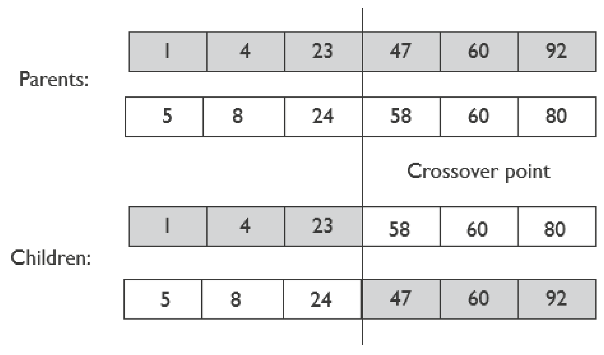
The crossover step creates a new generation of solutions from the initial population. For each child solution, a pair of parent solutions is selected, and single-point crossover is applied; that is, a random point on the parent chromosome is chosen, and segments before and after this point are swapped between parents to create two children. This is illustrated in Figure 2. This method allows child solutions to inherit characteristics (bands) from both parents.

Crossover is performed on a set percentage of the population, which is determined by the crossover rate. The crossover rate follows previous work and is set to 0.8 ([44]).

After generating new “parent” and “child” chromosomes, elitist selection retains the fittest individuals, maintaining a constant population size. This usually increases average fitness because only top performers are used for breeding. Next, during the mutation step, random genes are altered according to the mutation rate. We use a high mutation rate of 0.6 since this helps maintain diversity and prevent premature convergence [44]. Elitist selection is applied after mutation, ensuring that strong solutions are preserved so that inferior mutations do not replace better solutions.

The steps of the genetic algorithm are summarized in Figure 3.

2.3.5. Parameter Selection for Genetic Algorithm

The performance of the genetic algorithm relies strongly on parameter choices, particularly the crossover and mutation rates, which determine the portion of the population that undergoes these steps. High mutation rates help avoid premature convergence and local minima, as suggested in [44,45]. Similarly, [44] uses comparable crossover rates. In our work, smaller population sizes and fewer generations are required, likely aided by elitist selection to accelerate convergence.

Table 2. GA parameters.

Crossover rate	0.8
Mutation rate	0.6
Population size	10/20
Max generations	15–20

summarizes the parameters chosen for the evolution of the Genetic Algorithm. The selected parameter values are also close to those suggested in [46].

2.3.6. Fitness Function Modification for Multiclass Cases

In multiclass problems, such as ours with over 20 material classes, some materials are more challenging to discriminate than others. As a result, band subset selections may yield high overall discrimination but lower accuracy for certain classes. Maximizing a fitness function—often the mean classification accuracy—can advantage higher averages at the expense of underperforming classes. To guarantee a fairer discrimination accuracy over all material classes considered, we study the impact of different types of fitness functions:

• Default scheme:
  The fitness function computation is the mean classification accuracy for all material classes.
• Penalization scheme:
  This approach introduces a second term in the fitness computation to penalize the potential lack of equity in class accuracy caused by band selection. The first term in Equation (3) corresponds to the mean pixel accuracy per class (identical to Equation (2)), while the second term is the difference between the highest and lowest class classification accuracies, which is subtracted from the mean class accuracy. Both terms are divided by the total number of classes, N. Therefore, for any band subset $B_j$, the fitness is computed as:

  $$Fitness\left(j\right)= {\displaystyle \frac{\sum _{k=1}^{k=N}Accur\left(k\right)}{N}}-{\displaystyle \frac{({max}_{k=1\dots N}\left\{Accur\left(k\right)\right\}-{min}_{k=1\dots N}\left\{Accur\left(k\right)\right\})}{N}} for B_j\in \{1,\dots 101\}$$

  (3)
• Weight-based/prioritization scheme:
  Analysis shows that materials ABS, MDPE, ULDPE, LLDPE1, and LDPE2 (classes 11, 13, 19, 21, and 22) are the hardest to classify. About half of all materials reach high accuracy (>80%), but these five often fall below 50% when fewer bands are used. To improve performance, the fitness function assigns a weight of 1 to these challenging classes and 1/10 to others. The mean classification accuracy is then computed using Equation (4) by weighting the accuracy of all class materials by their corresponding class weight, W(k).

  $$\mathrm{W}\left(\mathrm{k}\right)=1fork\in \left\{\mathrm{11,13,19,21,22}\right\}$$

  $$\mathrm{W}\left(\mathrm{k}\right)=1/10fork \notin \left\{\mathrm{11,13,19,21,22}\right\}$$

  $$Fitness\left(j\right)={\displaystyle \frac{\sum _{k=1}^{k=NumClasses}W\left(k\right)\ast Accuracy\left(k\right)}{NumClasses}}for{B}_j\in \{1,\dots 101\}$$

  (4)
• Subset-based fitness computation 1:
  The band selection fitness is calculated using the classification accuracy for challenging materials ABS, MDPE, ULDPE, LLDPE1, and LDPE2 (classes 11, 13, 19, 21, and 22), as shown in Equation (5). This approach prioritizes accurate identification of these materials, while the classifier is still trained on all material classes.

  $$Fitness \left(j\right)={\displaystyle \frac{{\sum }_{k=\left\{\mathrm{11,13,19,21,22}\right\}}Accuracy\left(k\right)}{5}} for B_j\in \{1,\dots 101\}$$

  (5)
• Subset-based fitness computation 2:
  The band subset fitness is computed as the classification accuracy of the challenging materials, as given by Equation (5). The difference is that in this approach, the classifier model is only trained for these challenging classes.

2.3.7. Simulation of Broader Band Responses

Most studies on band relevance analysis rely on a high-spectral-resolution data set with hundreds of narrowband spectral responses. Similarly, we start from a 101-band data set with narrow spectral bands of 5 nm full-width-half-max (FWHM). In practice, however, we may want to extrapolate how the selection of the best narrow bands would translate to a sensor with fewer and broader bands. To study this, we mimic broader band responses by binning our spectral dataset over either three consecutive bands (33 bands of 15 nm width) or five consecutive bands (20 bands of 25 nm width). Figure 4 illustrates the band binning and the corresponding band numbering for the different bandwidth responses.

Table 3. Band conversion between data sets of different widths.

	To 5 nm Set F’ (101 Bands)	To 15 nm Set F’ (33 Bands)	To 25 nm Set F’ (20 Bands)
From 5 nm set F	F’= F	F’ = F/3	F’ = F/5
From 15 nm set F	F’ = 3 * F	F’ = F	F’ = ((3 * F) − 1)/5
From 25 nm set F	F’ = (5 * F) − 2	F’ = ((5 * F) − 2)/3	F’ = F

indicates the band conversion equation used to determine the central wavelengths F’ from the different initial data sets of central wavelengths F.

2.3.8. Benchmarking with Respect to State-of-the-Art Successive Projection Algorithm

We benchmark our Genetic Algorithm (GA) with respect to the Successive Projection Algorithm (SPA) [25] and use the more efficient algorithm implementation provided in [47]. In [34], the proposed deep learning band selection approach is compared with other band selection approaches, and the results show that SPA is the best-performing algorithm for some of the data sets. SPA starts from a given initial band and successively computes bands with minimum collinearity with the already selected bands. Therefore, for a low number of target bands (e.g., 3 and 4), we see that SPA is significantly influenced by the first band selection. For this reason, we test an approach in which the first band for SPA is provided by the GA selection of the best three bands. The aim is to initialize SPA with a known, relevant, and informative band instead of a random selection. We refer to this approach as GA-SPA. We also test the initialization of SPA using the relevant plastic absorption bands provided in [19].

3. Results and Discussion

In this section, the experimental results are presented by evaluating the impact of different parameters, such as population initialization, classifier method, and width of the spectral bands. Additionally, the adaptation of the fitness function in the multiclass scenario described in the previous section is evaluated.

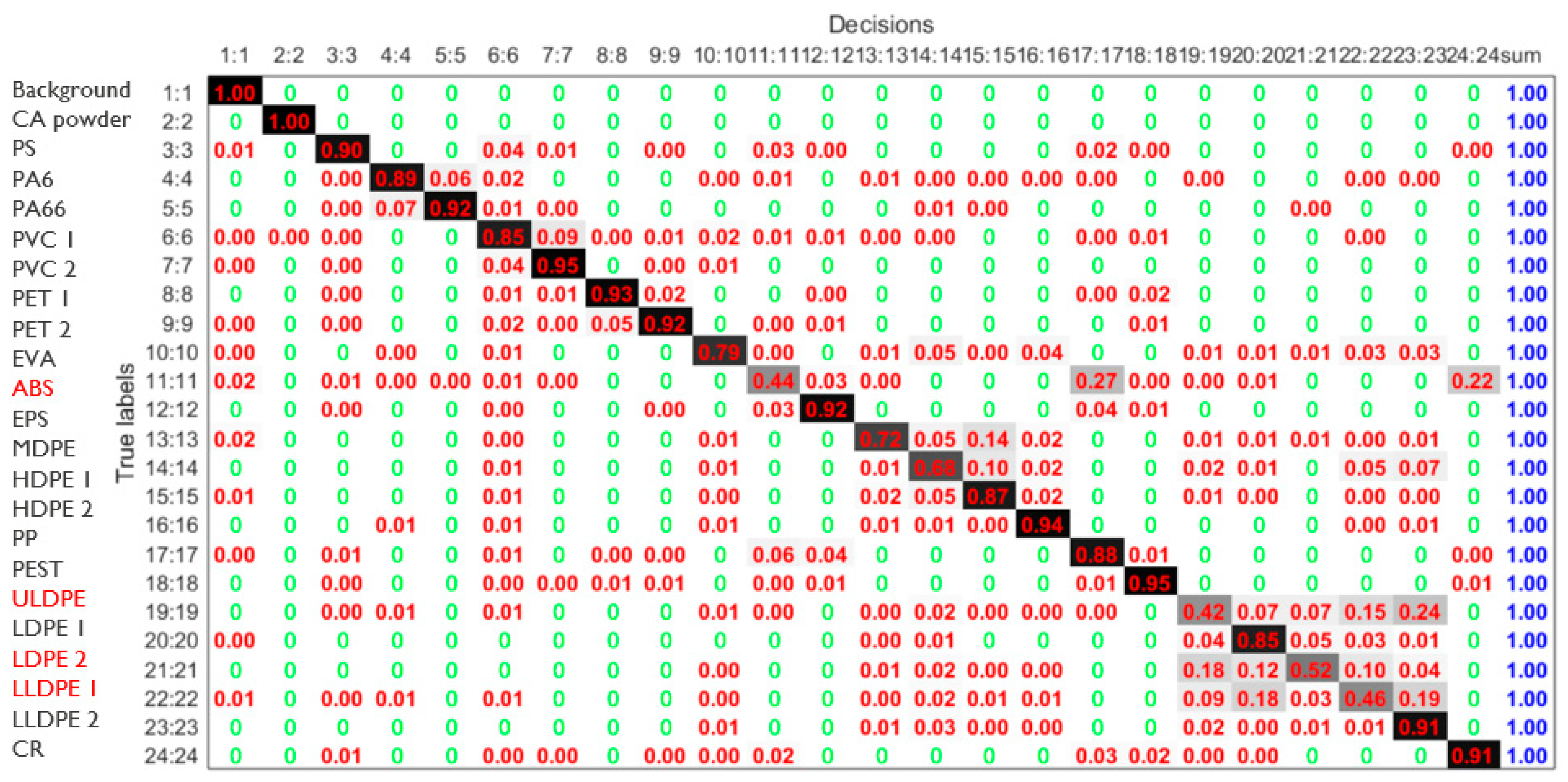
For the experimental work, a ROI is selected, covering around 60% of the microplastic beads, with 20% of the ROI pixels used for training and the remaining 80% for testing. This train/test set is used for all experimental comparisons of the different methods and parameters. Unless stated otherwise, the default classification method used is the quadratic discriminant classifier (QDC) with linear discriminant analysis (LDA) and median filtering 5 × 5 as a preprocessing step. Discrimination based on the initial 101 spectral bands of all tested materials is possible, achieving a mean pixel classification accuracy per material of 92%, with a minimum classification accuracy of 61% for LLDPE 1. After 15 GA iterations (population 10) on the train/test dataset and even population initialization, the resulting confusion matrix for the best nine bands achieved a mean pixel accuracy of 82.8% (see Figure 5).

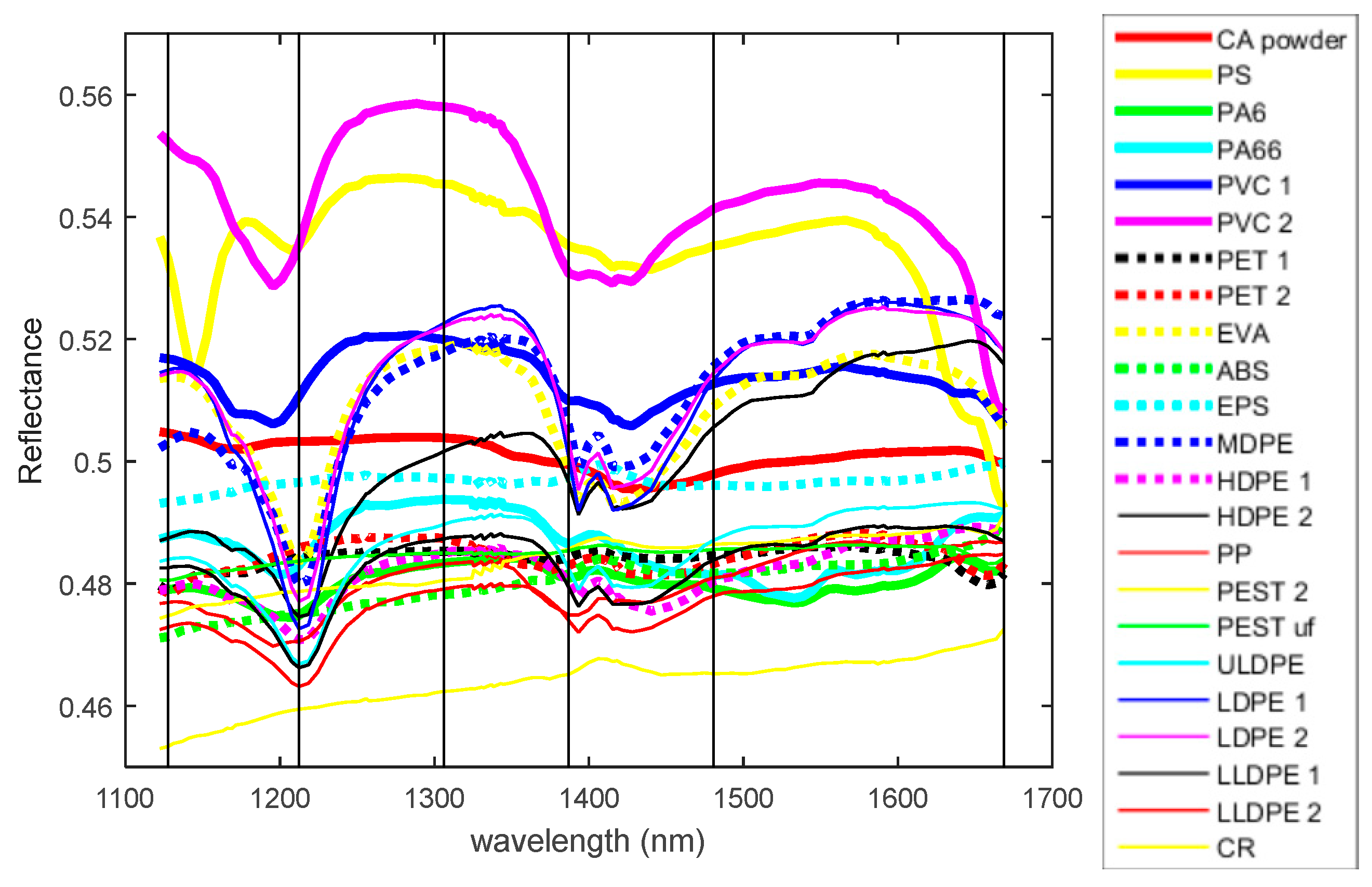
As mentioned in Section 2.3.6, the most challenging materials, reaching the lowest classification accuracies, are ABS, ULDPE, LDPE 2, LDPE 1, and MDPE. Figure 6 shows the mean spectral signatures of the different microplastic materials. We highlight with vertical lines the set of the best six bands found by the algorithm: 1.127, 1.212, 1.305, 1.386, 1.480, and 1.668 nm. As can be seen, they are quite evenly distributed over the spectral range.

Our set of the best nine bands, providing high accuracy for nearly all these 20 materials, includes 1.136, 1.218, 1.257, 1.330, 1.374, 1.393, 1.446, 1.514, and 1.668 nm (from an original range of 1100 to 1670 nm). Many of these bands coincide with those reported in the literature [19,20,48] as relevant absorption peaks in plastic materials.

Regarding sample morphology, the majority of samples are pellets, with four exceptions: EPS, PEST, CR, and CA. EPS consists of beads that share similar characteristics and homogeneity with pellets when observed under a microscope. PEST is in fabric form, and it was folded to offer more homogeneity. CR consists of homogeneous, flatter black rubber tire pieces, offering stable spectra. Only CA was in powder form, but it was equally homogeneous under the microscope. Although no clear effect of morphology could be observed in the acquired spectra, it would be interesting to assess the potential effect of material morphology (pellet, tissue, or powder) in a future study. We observed that all these non-pellet materials were easily discriminated, while the most challenging materials to discriminate were the few pellet types already mentioned.

Another aspect to be considered is that the samples used in this study are virgin samples, while real-world samples may be covered in dirt. Our experience in imaging larger plastic items shows that minor scratches or surface dirt rarely affect spectral-based discrimination unless the dirt forms a thick layer or covers the entire plastic surface. However, UV exposure and other types of degradation may alter the spectra of plastics, potentially reducing the model performance. While discrimination may still be feasible, training with degraded samples may be necessary to maintain optimal results.

3.1. Impact of Initialization with Even Distribution

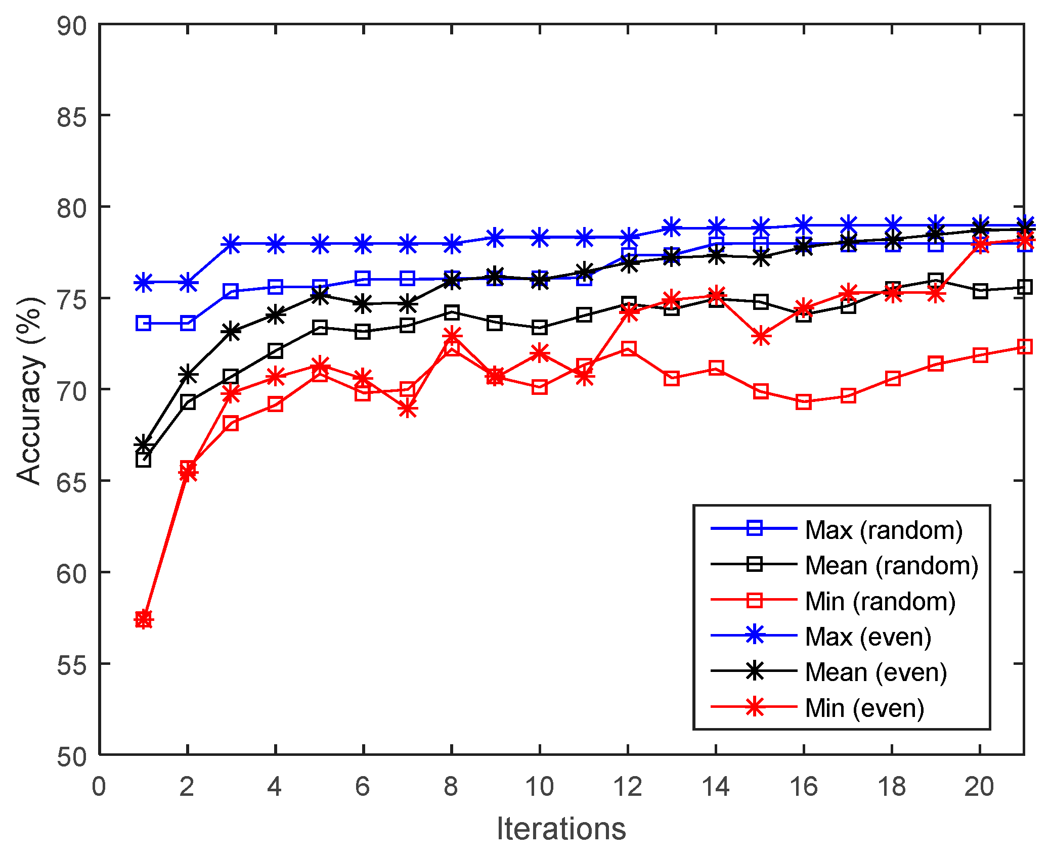
We start by comparing the potential impact of an initialization scheme that includes evenly distributed bands over the range with respect to a purely random initialization of the bands. Because larger populations of random solutions may have a higher chance of populating the entire band range, we compare both initialization methods for different population sizes. As a classifier method, a quadratic discriminant classifier (QDC) with LDA and median filtering 5 × 5 as preprocessing steps is used. Identical training and test sets are used for model building in all scenarios.

Table 4. Mean accuracy reached by random and evenly distributed initialization schemes.

Pop 10	Random init.	Distributed init.
Best three bands	61.5%	62.3%
Best six bands	78.1%	78.2%
Best nine bands	81.4%	82.9%
Pop 20	Random init.	Distributed init.
Best three bands	61.6%	61.6%
Best six bands	76.1%	78.3%
Best nine bands	82.4%	83.5%

shows the mean classification accuracies obtained for different target band sets. On average, higher mean classification accuracy is achieved when using an even initialization scheme, which corresponds to a better band selection made. We also study the convergence speed of the algorithm towards an optimal band selection. Figure 7 shows the fitness value (classification accuracy) of the 6-band selections obtained as a function of the algorithm iteration number. The highest (max) classification accuracy obtained within the population of band subsets is shown, together with mean values among band subsets and the worst band subset (minimum classification accuracy).

An even initialization of band subsets achieves higher average and maximum classification accuracies than random initialization, especially during early algorithm iterations. Random initialization only matches these results after iteration 12–14. Overall, even initialization speeds up convergence to optimal band selection and yields a higher mean accuracy across solutions.

Current works on Genetic Algorithms for band selection do not propose any other initialization strategy than random initialization [27,28,29,49]. Instead, we propose initializing the solution space with even band distributions. We have demonstrated that this approach speeds up convergence and reaches a band subset with higher classification accuracy.

3.2. Impact of Classifier Method on Band Selection

This section evaluates the effect of classifier choice on band selection. Since classifiers like linear, quadratic, or non-linear models may favor different optimal bands, we examine whether band selections tailored for one classifier work for others. We compare band selections and classification accuracies across different classifiers: Linear Discriminant Classifier (LDC), Quadratic Discriminant Classifier (LDA + QDC), and Random Forest (LDA+RF), considering both the method used for band extraction and for accuracy computation.

Table 5. Mean accuracy for different classifier models and band subset sizes.

Best Bands		LDC Model	LDA + QDC Model	LDA + RF Model
Best three bands	LDC generated	51.0%	59.2%	63.7%
	LDA + QDC generated	47.4%	62.1%	64.1%
	LDA + RF generated	49.5%	60.5%	66.3%
Best four bands	LDC generated	55.8%	66.8%	68.3%
	LDA + QDC generated	54.7%	69.5%	73.9%
	LDA + RF generated	54.9%	68.0%	71.9%
Best six bands	LDC generated	60.4%	76.7%	80.5%
	LDA + QDC generated	59.4%	78.2%	81.1%
	LDA + RF generated	58.5%	76.8%	80.0%
Best nine bands	LDC generated	62.9%	81.0%	78.9%
	LDA + QDC generated	62.0%	82.8%	83.1%
	LDA + RF generated	60.4%	82.3%	83.2%
Best 16 bands	LDC generated	66.3%	84.8%	78.7%
	LDA + QDC generated	62.7%	87.6%	83.3%
	LDA + RF generated	64.1%	85.2%	84.2%

Numbers in bold highlight the highest performance achieved.

shows the suitability of the band selection extracted by the genetic algorithm with classifier A (1st column, Table 5) when evaluated with classifier B (1st row, Table 5). A population size of 10 and 15 iterations is used for all classifier models. Identical train and test datasets are used for all classifier model building, and the random seed generation is fixed so that all random processes are identical for the different classifier models. Typically, more advanced classifier models, such as random forest (LDA + RF), result in higher classification accuracy than LDC or QDC classifiers. This is more noticeable when the number of bands selected is lower. In terms of execution cost, the LDC and QDC classifiers are comparable, but the RF classifier increases the execution time by a factor of roughly 23.

In addition, from the analysis in Table 5, we can observe the following:

• Band subsets generated by a particular classifier (LDC, QDC, or RF) tended to perform best when evaluated using the same classifier, as reflected by the highest classification accuracy (shown in bold).
• Band subsets selected using a quadratic classifier (QDC) yield higher accuracy for RF models than those selected by a linear discriminant classifier (LDC), likely because QDC better captures the non-linearity of RF. In some cases, QDC-selected bands even outperform or match the performance of band subsets generated specifically for RF.

We also tested the impact of a mixed approach, where the first 10 iterations were run with a simple classifier, such as LDC, and the next five iterations were run with another classifier (QDC or RF). The results are presented in

Table 6. Mean classification accuracy for pure and mixed approaches.

	LDC (15it)	LDA + QDC (15it)	LDA + RF (15 it)	LDA + QDC (10it + 5it)	LDA + RF (10it + 5it)
Best three bands	51.0%	62.1%	66.3%	60.6%	68.2%
Best four bands	55.8%	68.2%	74.3%	69.5%	76.2%
Best six bands	60.4%	78.2%	80.0%	76.2%	81.5%
Best nine bands	62.9%	82.8%	83.2%	81.7%	82.4%
Best 16 bands	66.3%	87.6%	84.2%	87.0%	82.4%

. This mixed approach provides comparable results (within 2%) with respect to a QDC pure approach (15 iter LDA + QDC). The speed-up obtained is marginal (~2% reduction in execution time). However, a mixed approach for the RF classifier achieves comparable or even slightly higher performance for a lower number of bands (<9), while reducing the total execution time of the genetic algorithm by 64%.

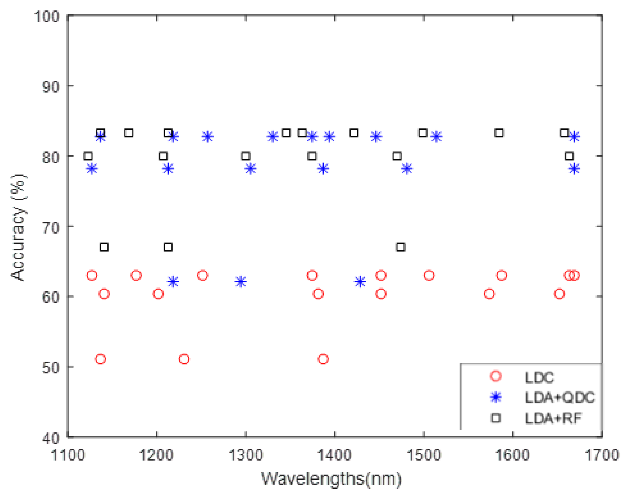
Figure 8 shows the final band selections generated by the GA with the different classifiers (LDC, QDC, and RF) and the resulting classification accuracy on the y-axis, corresponding to optimal 3, 6, and 9 band subsets. The best band selections found tend to spread across the full range for all classifiers and numbers of bands.

Within each classifier band selection, the bands selected in the 3-band subset tended to appear in the selected bands of the 6- and 9-subsets. Similarly, most of the bands in the 6-band subset also appear in the proximity of the 9-band selection. When comparing different classifiers, 3-band selections per classifier differ substantially; however, for higher band subsets, such as 6 or 9, more commonalities appeared in the band selection. The 1450–1540 nm range has the fewest band selections, as does the region around 1300 nm. Thus, band selection populates the regions 1120–1260 nm, 1340–1420 nm, and 1560–1660 nm. Most state-of-the-art works consider a single classifier, regardless of the band selection method [29,34,49]. Only [35] considered different classifier methods. However, band selection is performed in an unsupervised manner; therefore, the potential impact or suitability of the classifier method for a specific band selection is not evaluated.

In our work, the relationship between the classifier used in fitness computation and its effect on the final band selection was examined. Results presented in Table 5 indicate that the choice of classifier can influence which bands are identified as optimal for discrimination. Some plastic absorption bands tend to be selected as relevant, regardless of the classifier type. However, classifiers based on linear and non-linear relationships may require different information to perform optimally. As some absorption bands are relatively broad, the sets of optimal bands for different classifiers are similar but not identical (see Table 5). Consequently, using an optimal band subset derived from one classifier with a different classifier, results in slightly reduced classification accuracy.

3.3. Impact of Neighboring Band Selection

Spectral signatures in the SWIR range (1100–1700 nm) do not present sharp features for these materials, as the absorption bands are relatively broad. With 100 bands covering the 550 nm range (1100–1650 nm), there are consecutive bands every 5 nm, which could make the bands around a specific wavelength quasi-equivalent as a band selection. To verify this hypothesis, we replaced the algorithm-selected best subsets of bands “B” with adjacent bands within 5–20 nm. In other words, we replace the most adjacent band (B + 1, B − 1) with four bands away (B + 4, B − 4) and evaluate the suitability of the replaced set of bands in terms of discrimination accuracy. Replacing the optimal band subset with bands more than 10 nm away consistently reduces the classification accuracy, especially for subsets of only three or four bands. The farther the replacement bands are from the original selection, the greater the performance drop.

Table 7. Variation over mean accuracy (%) for bands adjacent to the optimal bands.

	Variation over Mean Pixel Accuracy (%) for LDA+QDC Classifier
	B	B + 1	B − 1	B + 2	B − 2	B + 3	B − 3	B + 4	B − 4
Best three bands	62.1%	+0.26	−1.52	−0.92	−3.08	−2.66	−5.36	−4.59	−7.43
Best four bands	68.2%	+0.17	+0.23	−1.48	−0.44	−3.83	−2.69	−5.94	−5.12
Best six bands	78.2%	−0.93	−1.32	−2.11	−1.86	−3.33	−2.42	−5.42	−3.13
Best nine bands	82.8%	+0.45	−0.72	−1.19	−1.60	−1.94	−2.44	−1.81	−3.32
Best 16 bands	87.6%	+0.33	−0.57	−1.05	−0.74	−0.85	−0.52	−1.86	−1.43

shows the results obtained when all bands are systematically replaced with the best band subset in the same way. We can see how replacing bands B by the directly next adjacent ones (B + 1, B − 1) provides slightly higher accuracies in 50% of the cases, but lower accuracy in the other 50% of the cases. Replacing the optimal band subset with bands more than 10 nm away consistently reduces the classification accuracy, especially for subsets of only three or four bands. The farther the replacement bands are from the original selection, the greater the performance drop.

Assessing the impact of selecting a neighboring band instead of the optimal band is crucial, as sensor fabrication processes frequently deviate from the central wavelength specifications. Consequently, it is relevant to evaluate in advance how this will affect the final system’s accuracy.

3.4. Impact of Width of Band Responses

The analysis presented so far was performed on 101 narrow spectral bands with a full width at half-maximum (FWHM) of 5 nm. We now mimic the impact of broader band responses by binning our spectral dataset over either three consecutive bands (33 bands of 15 nm width) or five consecutive bands (20 bands of 25 nm width). The GA is then run to find the best band selection starting from either the narrowband set (5 nm) or the broader-band sets (15 nm or 25 nm). Moreover, the performance of the narrowband dataset is evaluated on the broader band set, and vice versa. The results in terms of pixel accuracy achieved for the LDA+QDC classifier are shown in

Table 8. Mean pixel accuracy achieved with GA band selection.

		Accuracy on 5 nm Width	Accuracy on 15 nm Width	Accuracy on 25 nm Width
Best three bands	Selection from width = 5 nm	61.6%	64.3%	65.7%
	Selection from width = 15 nm	60.9%	64.3%	65.7%
	Selection from width = 25 nm	61.9%	63.8%	65.7%
Best six bands	Selection from width = 5 nm	78.9%	80.5%	81.5%
	Selection from width = 15 nm	76.6%	80.0%	82.4%
	Selection from width = 25 nm	76.0%	79.4%	81.8%
Best nine bands	Selection from width = 5 nm	83.5%	86.4%	88.0%
	Selection from width = 15 nm	82.3%	86.3%	88.2%
	Selection from width = 25 nm	82.8%	86.4%	88.8%

, and the optimal band sets are shown in

Table 9. Optimal bands for different spectral widths.

Original Bands	Best Three Bands	Best Six Bands	Best Nine Bands
101 bands of 5 nm	19-32-56	3-19-33-50-76-99	3-10-14-19-32-50-61-82-98
33 bands of 15 nm	7-11-19	5-7-11-19-25-33	2-4-7-13-17-21-23-28-33
20 bands of 25 nm	4-7-12	3-4-7-11-14-20	1-3-4-5-8-12-13-17-20

.

Spectral binning (wider bands) improves pixel classification accuracy; for example, 3-band grouping increases accuracy by 3%, with a further 1% gain using groups of five. This trend holds for the 6- and 9-band cases, where broader bands yield higher accuracy up to about 25 nm. Whether starting from narrow (5 nm) or wider band sets (15 or 25 nm), the optimal bands are generally consistent, although deviations increase when mapping broad bands back to narrow ones. Optimal bands selected from a dense set (100 bands at 5 nm each) also perform well on broader sets, but not always vice versa, because the central wavelength of a broader band may not match the true optimal narrow band.

Most current research [29,32,33,34,35] focuses on band selection from remote sensing applications with high-resolution spectral data sets (of at least 100 bands) and overlooks variations in spectral widths. In industrial contexts, where custom sensor development is feasible, diverse sensor configurations with varying numbers and widths of spectral bands are possible. Thus, it is important to assess how the width of a spectral band around a target wavelength impacts application outcomes. To our knowledge, this study is the first to simulate broadband responses from high-resolution narrowband data to compare optimal band selection across different spectral widths. Our findings show that a similar band selection can be achieved using either narrow or broad bands. However, translating selected bands from a narrow set to a broader band set is generally more straightforward than vice versa.

3.5. Impact of Prioritization Scheme to Steer Band Selection Towards More Balanced Multiclass Discrimination

We introduced several methods to achieve a more balanced classification accuracy across the material classes. In this respect, all the presented state-of-the-art methods [29,31,32,33,34,35] focus on maximizing average class accuracy (AA) or overall accuracy (OA), which can disadvantage harder-to-classify groups in multiclass data sets and limit the applicability of the solution found. To address this, we modified the fitness function to encourage even accuracy among all classes using the best 9-band, 6-band, and 3-band subsets.

Table 10. Impact of prioritization scheme on multiclass accuracy balance.

		Basic	Penalization	Weight	Subset 1	Subset 2
Best nine bands	Mean accuracy	83.3/45.5%	83.0/45.3%	82.5/46.1%	82.4/39.5%	81.8/44.2%
	Worst-4 accur	50.0%	50.3%	53.4%	51.0%	51.0%
	Materials < 50%	(2) abs, uldpe	(1) abs	(1) uldpe	(1) uldpe	(1) uldpe
Best six bands	Mean accuracy	78.4/34.0%	78.6/37.2%	77.2/34.2%	76.8/34.2%	76.1/28.8%
	Worst-4 accur	39.9%	41.77%	47.12%	47.1%	43.3%
	Materials < 50%	(4) lldpe1, abs, uldpe, ldpe2	(4) lldpe1, abs, uldpe, ldpe2	(2) uldpe, abs	(2) uldpe, abs	(2) uldpe, abs
Best three bands	Mean accuracy	60.8/8.8%	60.6/8.9%	60.7/9.3%	60.4/9.4%	59.6/12.7%
	Worst-4 accur	18.6%	19.6%	17.6%	17.3%	22.6%
	Materials < 50%	(8)	(7)	(8)	(7)	(6)

shows the classification accuracies obtained by the different approaches presented in Section 2.3.6 using the best 9-band, 6-band, and 3-band subsets.

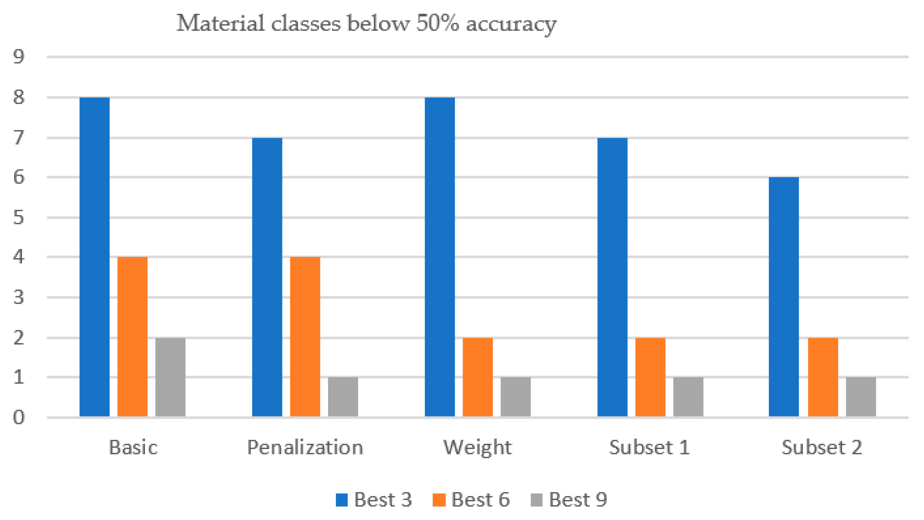
With respect to the basic method, the number of materials below 50% pixel accuracy is generally reduced (from 2 to 1 (9 bands), 4 to 2 (6 bands), and 8 to 6 (3 bands), which shows that the proposed methods succeed in improving the discrimination over the most challenging materials. This is illustrated in Figure 9.

Using these methods improves accuracy for the most challenging materials (such as LDPE1, ABS, ULDPE, LDPE2, and MDPE), with gains of 1–8% for the four toughest cases. This may come at the cost of a slightly lower overall mean accuracy. We can conclude that prioritizing metrics for difficult classes helps prevent their penalization during band selection.

3.6. Benchmarking with Successive Projection Algorithm (SPA)

Table 11. Comparison of GA and SPA approaches for different band numbers and classifier methods.

Method		LDC	LDA + QDC	LDA + RF	Band Number
Best three bands	SPA	41.9%	53.4%	56.7%	19-50-101
	GA-SPA	45.0%	60.1%	60.3%	18-32-101
	GA	47.4%	62.1%	64.1%	19-32-59
Best four bands	SPA	48.9%	66.7%	67.5%	19-42-50-101
	GA-SPA	51.1%	66.7%	70.0%	18-32-71-101
	GA	54.7%	69.5%	73.9%	2-19-72-100
Best six bands	SPA	54.0%	74.7%	76.8%	2-19-42-50-97-101
	GA-SPA	52.3%	71.9%	72.0%	18-32-42-71-96-101
	GA	59.4%	78.2%	81.1%	2-18-34-51-67-101
Best nine bands	SPA	60.0%	81.5%	79.9%	2-19-42-50-57-59-85-97-101
	GA-SPA	58.1%	80.9%	80.6%	2-4-18-32-42-59-71-96-101
	GA	62.0%	82.8%	83.1%	4-19-26-39-49-52-62-72-101
Best 16 bands	SPA	62.5%	86.3%	80.8%	2-4-12-14-19-32-40-42-50-57-59-60-85-97-99-101
	GA-SPA	63.2%	86.6%	81.8%	2-4-9-13-15-18-32-42-46-54-59-71-85-96-99-101
	GA	62.7%	87.6%	83.3%	1-9-15-19-21-32-38-44-50-56-62-68-71-89-95-101

compares the band selection obtained using different approaches: SPA, our GA, and the GA/SPA combined approach, where we initialize SPA with each of the best three bands found by our GA and show only the best-performing band selection. We evaluate the band selections using the average accuracy (AA) for our three classifiers: LDC, LDA + QDC, and LDA + RF. We also evaluated the initialization of SPA with relevant absorption bands in the literature [19,48], namely, 1212, 1289, and 1660 nm. However, initialization from our best GA bands provided better performance; therefore, we only reported the best results achieved. The combined approach GA-SPA improves accuracy over SPA for small band sets of three or four bands (2–7% increase). However, from six bands, it provides results similar to those of SPA or slightly decreases the accuracy. Our GA consistently achieves the best band selection in terms of accuracy for all three classifiers. GA outperforms SPA by 3.5–8.7% for small band subsets (3, 4, 6) and by 0.2–3.2% for larger sets (9, 16). Only in the 16-band LDC case does GA-SPA slightly surpass GA (by 0.5%). In all other scenarios, the GA outperforms both SPA and GA-SPA.

Both SPA and GA tend to produce band sets that are distributed over the entire spectral range of 1100 to 1660 nm, supporting the benefits of an even distribution initialization approach for GA. The main differences in band selection between SPA and GA occur for small band subsets (3, 4, and 6), which also correspond to the largest differences in accuracy. Since our GA outperforms the SPA approach in all cases, irrespective of the classifier used, this suggests that an unsupervised approach that minimizes collinearity may not necessarily be optimal in terms of discrimination capability.

Although less computationally intensive methods exist, such as the SPA implementation used for benchmarking, GAs are generally better suited for larger datasets. However, since band selection is typically performed once and can occur offline, maximizing discrimination has a higher priority than computational efficiency in these algorithms.

4. Conclusions and Outlook

We presented a genetic algorithm for band selection and applied it to a 22-class microplastic material discrimination case. The main conclusions of this paper are as follows:

• The proposed algorithm consistently outperforms the state-of-the-art benchmarked SPA algorithm, finding a subset between 6 and 9 bands with a classification accuracy above 80% for a set of 22 microplastic materials.
• The proposed initialization scheme with an even band distribution improves the convergence of genetic algorithms for band selection.
• Optimal band selection varies per classifier, with quadratic classifiers yielding better band selection results across different classifier models.
• Combining classifiers across algorithm phases can achieve better quality and efficiency trade-offs than a single advanced classifier.
• Replacing the optimal band subset with bands more than 10 nm away consistently reduces the classification accuracy, especially for subsets of only three or four bands.
• Similar band selection results were obtained from narrow or broader (up to 25 nm) band assumptions, although selections from narrower sets translated more easily to broader ranges.
• Our modified fitness computation scheme ensures a more balanced accuracy across material classes, thereby increasing the applicability of the algorithm.

Selecting an optimal band subset is essential for developing cost-effective multispectral sensors that accurately detect microplastic contamination while minimizing memory and processing requirements. Microplastics contaminate marine, freshwater, and terrestrial environments and the resulting human exposure to these substances causes potential health risks. Therefore, the development of cost-effective sensors for microplastic detection contributes to multiple SDGs: 3 (‘good health and well-being’), 6 (‘clean water and sanitation’) or 9 (‘industry, innovation, and infrastructure’). This study analyzes how sensor design factors, such as central wavelength shifts and bandwidth changes, and choices like classifier model selection affect detection accuracy, helping to predict real-world performance across varying imagers and models. We leave the assessment of the potential impact of real-world sample diversity in morphology and contamination degree on discrimination performance for future work.

References

1. Sustainable Production and Consumption. 2020. Available online: https://ec.europa.eu/jrc/en/research-topic/sustainable-production-and-consumption (accessed on 1 July 2024).
2. The World’s Plastic Pollution Crisis, Explained. Available online: https://www.nationalgeographic.com/environment/article/plastic-pollution (accessed on 1 July 2024).
3. Tomaselli, D. Automated Recycling System Using Computer Vision. ECE-498 Capstone Des. Proj. Advis. Prof. Cotter 2019. [Google Scholar]
4. Wang, Z.; Li, H.; Yang, X. Vision-based robotic system for on-site construction and demolition waste sorting and recycling. J. Build. Eng. 2020, 32, 101769. [Google Scholar] [CrossRef]
5. Thornton Hampton, L.M.; Bouwmeester, H.; Brander, S.M.; Coffin, S.; Cole, M.; Hermabessiere, L.; Mehinto, A.C.; Miller, E.; Rochman, C.M.; Weisberg, S.B. Research recommendations to better understand the potential health impacts of microplastics to humans and aquatic ecosystems. Microplast. Nanoplast. 2022, 2, 18. [Google Scholar] [CrossRef]
6. Mapping Exposure-Induced Immune Effects: Connecting the Exposome and the Immunome|EXIMIOUS Project|Fact Sheet|H2020|CORDIS|European Commission. Available online: https://cordis.europa.eu/project/id/874707 (accessed on 7 July 2024).
7. Tirkey, A.; Sheo, L.; Upadhyay, B. Microplastics: An overview on separation, identification and characterization of microplastics. Mar. Pollut. Bull. 2021, 170, 112604. [Google Scholar] [CrossRef]
8. Eduard, W.; Weinbruch, S.; Skogstad, A.; Skare, Ø.; Nordby, K.C.; Notø, H. Content of clinker and other materials in personal thoracic aerosol samples from cement plants estimated by scanning electron microscopy and energy-dispersive X-ray microanalysis. Ann. Work. Expo. Health 2023, 67, 990–1003. [Google Scholar] [CrossRef]
9. Primpke, S.; Christiansen, S.H.; Cowger, W.; De Frond, H.; Deshpande, A.; Fischer, M.; Holland, E.B.; Meyns, M.; O’Donnell, B.A.; Ossmann, B.E.; et al. Critical Assessment of Analytical Methods for the Harmonized and Cost-Efficient Analysis of Microplastics. Appl. Spectrosc. 2020, 74, 1012–1047. [Google Scholar] [CrossRef]
10. Sim, W.; Song, S.W.; Park, S.; Jang, J.I.; Kim, J.H.; Cho, Y.M.; Kim, H.M. Unveiling microplastics with hyperspectral Raman imaging: From macroscale observations to real-world applications. J. Hazard. Mater. 2024, 463, 132861. [Google Scholar] [CrossRef]
11. Meyers, N.; Catarino, A.I.; Declercq, A.M.; Brenan, A.; Devriese, L.; Vandegehuchte, M.; De Witte, B.; Janssen, C.; Everaert, G. Microplastic detection and identification by Nile red staining: Towards a semi-automated, cost-and time-effective technique. Sci. Total Environ. 2022, 823, 153441. [Google Scholar] [CrossRef]
12. Kamruzzaman, M.; ElMasry, G.; Sun, D.W.; Allen, P. Non-destructive prediction and visualization of chemical composition in lamb meat using NIR hyperspectral imaging and multivariate regression. Innov. Food Sci. Emerg. Technol. 2012, 16, 218–226. [Google Scholar] [CrossRef]
13. Gonzalez, P.; Pichette, J.; Vereecke, B.; Masschelein, B.; Krasovitski, L.; Bikov, L.; Lambrechts, A. An extremely compact and high-speed line-scan hyperspectral imager covering the SWIR range. In Image Sensing Technologies: Materials, Devices, Systems, and Applications V; SPIE: Bellingham, WA, USA, 2018; Volume 10656, p. 106560L. [Google Scholar] [CrossRef]
14. Blanch-Perez-del-Notario, C.; Luthman, S.; Lefrant, R.; Gonzalez, P.; Lambrechts, A. Compact high-speed snapshot hyperspectral imager in the SWIR range (1.1–1.65 nm) and its potential in sorting/recycling industry. In Algorithms, Technologies, and Applications for Multispectral and Hyperspectral Imaging XXVIII; SPIE: Bellingham, WA, USA, 2022; Volume 12094, pp. 47–55. [Google Scholar]
15. Khan, M.J.; Khan, H.S.; Yousaf, A.; Khurshid, K.; Abbas, A. Modern trends in hyperspectral image analysis: A review. IEEE Access 2018, 6, 14118–14129. [Google Scholar] [CrossRef]
16. Serranti, S.; Fiore, L.; Bonifazi, G.; Takeshima, A.; Takeuchi, H.; Kashiwada, S. Microplastics characterization by hyperspectral imaging in the SWIR range. SPIE Future Sens. Technol. 2019, 11197, 134–140. [Google Scholar]
17. Faltynkova, A.; Wagner, M. Developing and testing a workflow to identify microplastics using near infrared hyperspectral imaging. Chemosphere 2023, 336, 139186. [Google Scholar] [CrossRef]
18. Faltynkova, A.; Johnsen, G.; Wagner, M. Hyperspectral imaging as an emerging tool to analyze microplastics: A systematic review and recommendations for future development. Microplast. Nanoplast. 2021, 1, 13. [Google Scholar] [CrossRef]
19. Alboody, A.; Vandenbroucke, N.; Porebski, A.; Sawan, R.; Viudes, F.; Doyen, P.; Amara, R. A New Remote Hyperspectral Imaging System Embedded on an Unmanned Aquatic Drone for the Detection and Identification of Floating Plastic Litter Using Machine Learning. Remote Sens. 2023, 15, 3455. [Google Scholar] [CrossRef]
20. Tamin, O.; Moung, E.G.; Dargham, J.A.; Yahya, F.; Omatu, S. A review of hyperspectral imaging-based plastic waste detection state-of-the-arts. Int. J. Electr. Comput. Eng. 2023, 13, 3407–3419. [Google Scholar] [CrossRef]
21. Rogers, M.; Blanc-Talon, J.; Urschler, M.; Delmas, P. Wavelength and texture feature selection for hyperspectral imaging: A systematic literature review. Food Meas. 2023, 17, 6039–6064. [Google Scholar] [CrossRef]
22. Mahieu, B.; Qannari, E.M.; Jaillais, B. Extension and significance testing of Variable Importance in Projection (VIP) indices in Partial Least Squares regression and Principal Components Analysis. Chemom. Intell. Lab. Syst. 2023, 242, 104986. [Google Scholar] [CrossRef]
23. Tibshirani, R. Regression shrinkage and selection via the lasso. J. R. Stat. Soc. 1996, 58, 267–288. [Google Scholar] [CrossRef]
24. Robin Genuer, R.; Poggi, J.M.; Tuleau-Malot, C. Variable selection using random forests. Pattern Recognit. Lett. 2010, 31, 2225–2236. [Google Scholar] [CrossRef]
25. Araújo, M.C.U.; Saldanha, T.C.B.; Galvão, R.K.H.; Yoneyama, T.; Chame, H.C.; Visani, V. The successive projections algorithm for variable selection in spectroscopic multicomponent analysis. Chemom. Intell. Lab. Syst. 2001, 57, 65–73. [Google Scholar] [CrossRef]
26. Goldberg, D.E.; Holland, J.H. Genetic algorithms and machine learning. Mach. Learn. 1988, 3, 95–99. [Google Scholar] [CrossRef]
27. Saqui, D.; Saito, J.H.; Jorge, L.A.D.C.; Ferreira, E.J.; Lima, D.C.; Herrera, J.P. Methodology for Band Selection of Hyperspectral Images Using Genetic Algorithms and Gaussian Maximum Likelihood Classifier. In Proceedings of the 2016 International Conference on Computational Science and Computational Intelligence (CSCI), Las Vegas, NV, USA, 15–17 December 2016; pp. 733–738. [Google Scholar] [CrossRef]
28. Nagasubramanian, K.; Jones, S.; Sarkar, S.; Singh, A.K.; Singh, A.; Ganapathysubramanian, B. Hyperspectral band selection using genetic algorithm and support vector machines for early identification of charcoal rot disease in soybean stems. Plant Methods 2018, 14, 86. [Google Scholar] [CrossRef] [PubMed]
29. Zhao, H.; Bruzzone, L.; Guan, R.; Zhou, F.; Yang, C. Spectral-Spatial Genetic Algorithm-Based Unsupervised Band Selection for Hyperspectral Image Classification. IEEE Trans. Geosci. Remote Sens. 2021, 59, 9616–9632. [Google Scholar] [CrossRef]
30. Tschannerl, J.; Ren, J.; Zabalza, J.; Marshall, S. Segmented Autoencoders for Unsupervised Embedded Hyperspectral Band Selection. In Proceedings of the 2018 7th European Workshop on Visual Information Processing (EUVIP), Tampere, Finland, 26–28 November 2018; pp. 1–6. [Google Scholar] [CrossRef]
31. Moharram, M.A.; Sundaram, D.M. Adaptive feature selection for hyperspectral image classification based on Improved Unsupervised Mayfly Optimization Algorithm. Earth Sci. Inform. 2024, 17, 4145–4159. [Google Scholar] [CrossRef]
32. Ayna, C.O.; Mdrafi, R.; Du, Q.; Gurbuz, A.C. Learning-Based Optimization of Hyperspectral Band Selection for Classification. Remote Sens. 2023, 15, 4460. [Google Scholar] [CrossRef]
33. Feng, J.; Gao, Q.; Shang, R.; Cao, X.; Bai, G.; Zhang, X.; Jiao, L. Multi-agent deep reinforcement learning for hyperspectral band selection with hybrid teacher guide. Knowl.-Based Syst. 2024, 299, 112044. [Google Scholar] [CrossRef]
34. Rahman, M.; Teng, S.W.; Murshed, M.; Paul, M.; Brennan, D. BSDR: A Data-Efficient Deep Learning-Based Hyperspectral Band Selection Algorithm Using Discrete Relaxation. Sensors 2024, 24, 7771. [Google Scholar] [CrossRef]
35. Mou, L.; Saha, S.; Hua, Y.; Bovolo, F.; Bruzzone, L.; Zhu, X.X. Deep reinforcement learning for band selection in hyperspectral image classification. IEEE Trans. Geosci. Remote Sens. 2021, 60, 1–14. [Google Scholar] [CrossRef]
36. Blanch-Perez-del-Notario, C.; Azari, A.; Jayapala, M.; Lambrechts, A. Microplastic discrimination with hyperspectral imaging. In Proceedings of the 14th IEEE GRSS Workshop on Hyperspectral Image and Signal Processing, (WHISPERS), Helsinki, Finland, 9–11 December 2024; pp. 1–5. [Google Scholar] [CrossRef]
37. MS-200-SHORT-RV|SEIWA Optical. Available online: https://www.seiwaamerica.com/product/camera-tube/ms-200-twl/ms-200-short-rv (accessed on 21 August 2025).
38. Matlab. The Mathworks, Natick. 2019. Available online: https://mathworks.com (accessed on 20 June 2020).
39. PerClass BV 2008–2022, Delft, NL. Available online: http://perclass.com/perclass-toolbox/product (accessed on 15 January 2018).
40. Naes, T.; Isaksson, T.; Fearn, T.; Davies, T. A User-Friendly Guide to Multivariate Calibration and Classification; NIR Publications: Chichester, UK, 2004. [Google Scholar]
41. Gonzalez, R.C.; Woods, R.E. Digital Image Processing; Prentice-Hall: Eaglewood Cliffs, NJ, USA, 2002. [Google Scholar]
42. Holland, J. Genetic algorithms. Sci. Am. 1992, 267, 66–73. [Google Scholar] [CrossRef]
43. Blanch-Perez-del-Notario, C.; Baert, R.; D’Hondt, M. Multi-objective genetic algorithm for task assignment on heterogeneous nodes. Int. J. Digit. Multimed. Broadcast. 2012, 2012, 716780. [Google Scholar]
44. Camelo, M.; Donoso, Y.; Castro, H. MAGS—An approach using multi-objective evolutionary algorithms for grid task scheduling. Int. J. Appl. Math. Inform. 2011, 5, 117–126. [Google Scholar]
45. Iosifidis, Y.; Mallik, A.; Mamagkakis, S.; De Greef, E.; Bartzas, A.; Soudris, D.; Catthoor, F. A framework for automatic parallelization, static and dynamic memory optimization in MPSoC platforms. In Proceedings of the 47th Design Automation Conference, (DAC ’10), Anaheim, CA, USA, 13–18 June 2010; pp. 549–554. [Google Scholar]
46. Zomaya, A.Y.; Ward, C.; Macey, B. Genetic scheduling for parallel processor systems: Comparative studies and performance issues. IEEE Trans. Parallel Distrib. Syst. 1999, 10, 795–812. [Google Scholar] [CrossRef]
47. Han, M. Successive Projections Algorithm (SPA) for Variable Selection. 2024. Available online: https://mingqianghan.github.io/posts/2024/10/variable-selection-spa%20/ (accessed on 9 July 2025).
48. Tasseron, P.; Van Emmerik, T.; Peller, J.; Schreyers, L.; Biermann, L. Advancing floating macroplastic detection from space using experimental hyperspectral imagery. Remote Sens. 2021, 13, 2335. [Google Scholar] [CrossRef]
49. Chen, W.; Zhi, X.; Hu, J.; Yu, L.; Han, Q.; Zhang, W. Genetic Algorithm-Based Weighted Constraint Target Band Selection for Hyperspectral Target Detection. Remote Sens. 2025, 17, 673. [Google Scholar]
Figure 1. SnapScan SWIR camera with reflectance microscope (left) and plastic pellets (right).
Sustainability 17 08123 g001
Figure 2. Single-point crossover.
Sustainability 17 08123 g002
Figure 3. Scheme of genetic algorithm.
Sustainability 17 08123 g003
Figure 4. Binning of band responses to emulate broader bands. Central bands are highlighted in a different color.
Sustainability 17 08123 g004
Figure 5. Confusion matrix for the best 9-band subset.
Sustainability 17 08123 g005
Figure 6. Mean spectral signatures of microplastic materials.
Sustainability 17 08123 g006
Figure 7. Max/mean/min accuracies versus iteration for random and even initialization schemes.
Sustainability 17 08123 g007
Figure 8. Band selection according to the classifier method.
Sustainability 17 08123 g008
Figure 9. Number of material classes below 50% accuracy for the different approaches and band subsets.
Sustainability 17 08123 g009