Article

Application of Machine Learning Approaches to Predict Soil Element Background Concentration at Large Region Scale

Technical Centre for Soil, Agriculture and Rural Ecology and Environment, Ministry of Ecology and Environment, Beijing 100012, China
*
Authors to whom correspondence should be addressed.
Sustainability 2025, 17(17), 7853; https://doi.org/10.3390/su17177853
Submission received: 4 July 2025 / Revised: 27 August 2025 / Accepted: 27 August 2025 / Published: 31 August 2025

Abstract

Soil element background concentration is foundational data for environmental quality assessment, contamination diagnosis, and sustainable land management. However, existing investigation-based methods are time-consuming and inefficient. The machine learning (ML) method has demonstrated excellent performance in predicting soil heavy metal concentration. In this study, based on the nine environmental variables of soil formation from 210 soil monitoring points, including elevation, pH, organic matter, soil type, parent material, plant cover, land use type, topography, and soil texture, decision tree (DT), random forest (RF), extreme gradient boosting (XGB), and support vector machine (SVM) models were used to predict the eleven soil element background concentrations. Among them, SVM and RF models could be used for an effective prediction of the background concentration of all soil heavy metals. Compared with the XGBoost and DT, the SVM for all heavy metals except for cadmium (Cd) and manganese (Mn) performs best. Although the key factors affecting background concentrations vary among different soil elements, organic matter, soil type, and altitude, they play a crucial role in the accurate prediction of soil element background concentration. This study provides simple and efficient ML models for predicting soil element background concentration at the large regional scale. The results of this study can be utilized to distinguish natural geochemical processes from human-induced pollution.

1. Introduction

Soil element background concentrations, representing natural elemental abundances unaffected by anthropogenic activities, are essential benchmarks for environmental quality assessment, contamination diagnosis, and sustainable land management [1]. Establishing accurate background values is crucial for distinguishing natural geochemical processes from human-induced pollution, especially in regions with complex geology or long-term agricultural and industrial histories [2]. With the increasing adoption of stringent soil protection policies worldwide, there is an urgent demand for robust and scalable frameworks capable of mapping background concentrations with high precision and mechanistic insight [3]. Two primary approaches exist for obtaining soil element background concentrations: geochemical and statistical methods [4]. Geochemical methods, also known as empirical methods, involve sampling from sites minimally impacted by industrial activities or considered relatively pristine [5]. In contrast, statistical methods are more widely used, not only to estimate background concentrations but also to separate geochemical anomalies from the background levels [6]. Regardless of methodological approaches, establishing reliable soil element background concentrations fundamentally lies in identifying reference areas with minimal anthropogenic influence. This critical prerequisite has become substantially more challenging in the Anthropocene era [7]. If soil element background concentrations could be accurately predicted by modeling, many challenges associated with locating suitable reference sites could be effectively addressed.
While substantial research has focused on developing predictive models for soil element concentrations, less attention has been paid to establishing reliable background values [8]. Traditional statistical approaches, such as general linear models (GLMs) and stepwise regression techniques, have been applied to predict heavy metal fraction, but also oversimplify the complex interdependencies among geological substrates, pedogenic processes, climatic, and topographic factors [9]. As established in foundational pedological studies [10,11,12,13], soil formation emerges from the dynamic interplay of climatic, parent material, geomorphology, biological activity, anthropogenic factors, and temporal evolution. Each factor exerts scale-dependent control over elemental distributions within soils. This multidimensional complexity results in spatially non-stationary relationships between elemental distributions and their environmental drivers—a challenge that conventional linear models, which assume spatial homogeneity and constant variance structures, are ill-equipped to address [8,14].
Recent advances in machine learning (ML) have transformed soil constituent prediction by capturing nonlinear dependencies and automating feature selection from multi-source geospatial data [15]. ML algorithms like random forest (RF) and extreme gradient boosting (XGBoost) have demonstrated outstanding performance in mapping soil heavy metal contamination driven by natural and socioeconomic factors [16,17,18,19,20]. However, their application to predicting soil element background concentrations remains limited, particularly in separating lithogenic contributions from diffuse anthropogenic signals [21]. Existing research tends to focus on pollution prediction rather than background modeling, often neglecting the challenges of distinguishing natural variability—such as weathering intensity, parent material composition, and hydrological redistribution—from human perturbations [22]. Additionally, most ML-based soil models predict total elemental concentrations without explicitly addressing the background-anomaly distinction, thereby restricting their applicability in regulatory contexts.
This study firstly addresses these gaps by evaluating four ML algorithms, including decision tree (DT), RF, XGBoost and support vector machine (SVM), for predicting soil element background concentrations, which exhibited excellent data mining capabilities and superior robustness against extreme values and noise [23]. Unlike prior approaches, our framework explicitly incorporates nine key soil-forming factors, innovatively integrating domain knowledge with data-driven feature engineering. The primary objectives of this research consist of the following: (1) compare the performance of these ML models optimized for soil element background concentrations prediction across diverse lithological and climatic regimes; (2) establish a framework to quantify the relative contributions of parent material composition, climatic weathering, and topographic redistribution to natural elemental abundances; and (3) create adaptable soil element background concentration maps to support region-specific environmental management strategies, using China’s Jiangxi Province as a testbed—a region characterized by complex metamorphic terrains. Our methodology bridges geochemical big data and actionable environmental insights, offering a scalable template for global soil element background concentration assessments amid anthropogenic global change. This work advances scientific understanding of pedosphere evolution while delivering practical tools for pollution source apportionment, ecological risk zoning, and sustainable soil governance.

2. Materials and Methods

2.1. Study Area and Data Sources

Jiangxi Province is located in eastern China, between 30°45′ and 35°20′ N latitude and 116°18′ and 121°57′ E longitude (Figure 1). The terrain is predominantly flat, gently sloping from the northwest to the southeast, and mainly composed of alluvial plains with scattered hills and coastal sandbars. The average elevation is below 50 m, positioning the province in a transitional zone between northern and southern China in terms of geography and ecology. The region experiences a monsoon-dominated climate that transitions between subtropical and warm temperate zones. Annual mean temperature ranges from 13.6 °C to 16.1 °C, with annual precipitation varying between 800 and 1200 mm. Prolonged processes of weathering, leaching, and sedimentation have resulted in a diverse array of soil types.
According to regional soil surveys and classification, the dominant soil types in the study area include red soil, paddy soils, yellow soil, yellow-brown soil, and purple soil, with localized distributions of brown soils and limestone soils. Soil development is controlled by parent material, hydrological conditions, topography, and anthropogenic influences. The spatial distribution of soil elemental background values exhibits marked regional variation, driven by complex interactions among pedogenic environment, soil classification, and historical land use types.
This study focused on Jiangxi Province, utilizing data from a systematic soil survey conducted between 1987 and 1988, as documented in the monograph Study on Soil Environmental Background Values in Jiangxi Province [24]. In this systematic soil survey, researchers excavated a total of 210 profiles and collected 556 soil samples. During the sampling process, at each sampling point, elevation, plant cover, land use type, topography, and soil texture in each layer of the profile were recorded. Moreover, soil type and parent material were obtained from the soil map of Jiangxi Province (scale 1:1 M) and the geological map of Jiangxi Province (scale 1:500 k). A total of 2310 records were measured from 210 soil monitoring sites, covering 11 heavy metals: arsenic (As), cadmium (Cd), cobalt (Co), chromium (Cr), copper (Cu), mercury (Hg), manganese (Mn), nickel (Ni), lead (Pb), vanadium (V), and zinc (Zn), along with associated numeric environmental variables including pH and organic matter. The contents of Zn and Cr were determined by atomic absorption spectrometry. The content of Cd was determined by the GFU-202 type Cd flameless method. The contents of Cu, Mn, Ni, Co, and Pb were determined by the flame method. The content of As was determined by diethyldithiocabamate (DDTC) spectrophotometric method, the content of V was determined by 721 spectrophotometry, and the content of Hg was determined by a cold atomic absorption mercury analyzer. All heavy metal content was reported in mg/kg. Elevation was expressed in meters, and organic matter was given as a percentage (%). The remaining environmental variables were dimensionless.

2.2. Theoretical Framework

Figure 2 illustrates the comprehensive framework for forecasting soil element background concentrations through ensemble machine learning models. This framework comprises three key steps: (1) data processing of input variables, (2) prediction model development, and (3) model applicability evaluation.

2.3. Digitization of Environmental Variables

To construct a digitized input matrix for predicting soil element background concentrations, this study adopted the variable digitization method proposed by He et al. [24], which transforms environmental variables into numerical forms. Specifically, each environmental variable was first categorized into discrete statistical units based on its intrinsic attributes. These units were designed to effectively characterize regional soil properties under the comprehensive environmental influences, while also meeting the fundamental statistical analysis prerequisites. The digitization procedure specifically aimed to quantitatively encode the hierarchical variations in environmental determinants through standardized numerical representations.
Among the nine environmental variables considered in this study, three were initially numeric variables (elevation, pH, and organic matter). The remaining six, including soil type, parent material, plant cover, land use type, topography, and soil texture, were categorical variables.
To eliminate the influence of dimensional inconsistency among variables, all input environmental variables were normalized to a unified scale using min-max normalization. This approach transforms all variables to a comparable range [0, 1], ensuring equal weight and fair comparison across features during model training. The normalization was performed using the following Equation (1):
X i ¯ = X i X min X max X min
where X i ¯ represents the normalized value, X i denotes the original input, and X min and X max signify the minimum and maximum values of the corresponding variable.

2.4. Identification of Environmental Variables Importance

According to the soil genesis theory, soil formation and development are controlled by five fundamental factors: climate, topography, parent material, biological activity, and time [25]. With the intensification of anthropogenic influences on the environment, increasing attention has been paid to the geochemical behavior of heavy metals that are closely related to both public health and ecological safety during soil formation. The migration and transformation of these elements are strongly influenced by soil environmental conditions and pedogenic processes, ultimately affecting the biogeochemical cycling of substances within the soil system.
The nine environmental variables selected in this study represent a comprehensive coverage of five classic soil-forming factors, along with anthropogenic influences. These variables may exert varying levels of influence and may be affected by multicollinearity. Therefore, principal component analysis (PCA) and multiple linear regression (MLR) were employed to identify the key environmental factors influencing soil elemental background values. PCA facilitates the elimination of highly correlated variables and assigns relative weights to each factor based on its contribution. MLR compares the magnitudes of the effects of independent variables on the dependent variable by using standardized regression coefficients.
PCA transforms high-dimensional data into a reduced set of principal components that capture the significant patterns of variation in the original dataset, while preserving as much information as possible. Prior to PCA, the Kaiser–Meyer–Olkin (KMO) test and Bartlett’s test of sphericity were conducted to evaluate the suitability of the data for factor analysis. Key influencing factors and their relative weights were determined based on eigenvalues and cumulative variance explained. MLR quantitatively describes the relationship between the independent variable X and the dependent variable Y through the regression function.

2.5. Machine Learning Models

Machine learning models, especially RF and XGBoost, have proven effective in accurately determining heavy metal background values in soil [17]. Xu et al. 2025 [26] proposed a comprehensive prediction framework, which employs an integrated model combining RF, SVM, and XGBoost models to conduct a high-resolution spatial prediction of soil heavy metal concentrations. The DT model, serving as a fundamental machine learning approach, has been extensively utilized as a reference model in comparative studies of heavy metal prediction in soils [27]. Therefore, to determine the most reliable approach for geochemical baseline prediction, this study conducted a comparative analysis of four machine learning algorithms (RF, SVM, XGBoost, and DT) in quantifying soil heavy metal background values.

2.5.1. Decision Tree

The decision tree (DT) is a supervised learning algorithm that recursively partitions the input feature space using a tree-structured model defined by decision rules, thereby enabling the prediction of the target variable [28]. The model consists of a root node, internal nodes, and leaf nodes. The root node represents the entire dataset and initiates the first split based on the most informative feature, while internal nodes further subdivide the data according to subsequent decision rules. The leaf nodes produce the final output, making the DT applicable to both classification and regression tasks [29].
For regression tasks, the prediction at each terminal node is typically calculated as the average of the observed values within that node, as expressed in Equation (2):
y ^ ( x ) = 1 N m i ϵ R m y i
where y ^ ( x ) represents the predicted value for input x, R m denotes the region corresponding to the mth leaf node, N m signifies the number of samples in that node, and y i denotes the actual values of the samples.
The construction of the DT model typically involves three main stages: feature selection, tree generation, and pruning. In this study, hyperparameters such as the maximum tree depth and minimum number of samples per leaf were tuned to optimize model performance. Model implementation and training were conducted using the Scikit-learn library in Python 3.13.5.

2.5.2. Random Forest

Random forest (RF), proposed by Breiman [30], is a classical ensemble learning algorithm that enhances predictive performance by aggregating multiple decision trees trained on bootstrapped samples. Each tree is independently constructed using a random subset of the training data. At each node, a randomly selected subset of features is considered to determine the optimal split. This strategy reduces variance and improves robustness against overfitting [31,32].
For regression tasks, the output of RF is computed by averaging the outputs of all individual trees (Equation (3)):
y = 1 n tree i = 1 n tree f ^ i ( x )
where y represents the predicted value for input x, f ^ i ( x ) signifies the output of the ith regression tree, and n tree denotes the total number of trees.
In this study, RF was implemented in regression mode. Key hyperparameters, including the minimum number of samples required to split a node, the minimum number of samples per leaf, and the maximum tree depth, were tuned to enhance model performance. The model was implemented using the Scikit-learn library in Python.

2.5.3. Extreme Gradient Boosting

Extreme gradient boosting (XGBoost) is an advanced ensemble learning algorithm based on the gradient boosting framework. Known for its high efficiency, regularization capabilities, and superior generalization performance, it is widely adopted for modeling complex, nonlinear relationships [33]. The method iteratively constructs a series of weak learners—typically CART regression trees—each trained to minimize the residual errors of the preceding model, thereby producing a robust predictive ensemble.
A key feature of XGBoost is its use of a second-order Taylor series approximation of the objective function, which enhances both computational efficiency and optimization accuracy. To prevent overfitting, the algorithm incorporates both L1 (Lasso) and L2 (Ridge) regularization terms within the objective function, effectively controlling model complexity [34].
The prediction function of XGBoost is expressed as Equation (4):
y = j = 1 J w j f j ( x ) + b
where y represents the predicted output for input x, fj (x) represents the output of the jth regression tree, wj denotes its associated weight, and b is the bias term. Each fj corresponds to a CART structure with decision branches and leaf nodes [35].
In this study, key hyperparameters, including maximum tree depth, minimum child weight, and the L1 regularization coefficient, were tuned to enhance predictive performance and model stability. All modeling procedures were implemented using the XGBoost package in Python.

2.5.4. Support Vector Machine

Support vector machine (SVM) is a supervised learning algorithm grounded in statistical learning theory, originally proposed by Cortes and Vapnik [36] and further elaborated by Vapnik [37]. It has been widely applied to both classification and regression tasks. The core idea is to construct an optimal hyperplane that maximizes the margin between classes in the feature space, thereby improving generalization. For nonlinearly separable data, SVM employs the kernel trick to implicitly map input features into a higher-dimensional space, enabling linear separation and modeling of complex nonlinear patterns.
For regression tasks, the model estimates a function of the following form (Equation (5)) [37]:
s ( X i ) = t = 1 T w t φ t ( X i ) + b
where s ( X i ) denotes the predicted value for input X i , φ t ( X i ) represents the nonlinear mapping function, and w t and b signify model parameters learned through training. The kernel function k ( X i , X j ) represents the inner product in the transformed space, which replaces the need for explicit nonlinear mapping.
In this study, the Radial Basis Function kernel was selected due to its strong ability to handle nonlinear data, which is defined as Equation (6) [38,39]:
k ( X i , X j ) = exp ( γ X i X j 2 )
Three key hyperparameters were optimized to enhance model performance: the penalty parameter C, the epsilon-insensitive loss term ε, and the kernel width γ. All modeling procedures were conducted using the Scikit-learn package in Python.

2.6. Model Implementation and Performance Evaluation

To systematically evaluate the predictive performance of different machine learning algorithms in estimating soil elemental background values, a scenario-based modeling framework was developed in this study. Four widely used algorithms were selected: DT, RF, XGBoost, and SVM. Two input variable selection strategies were considered: (1) unfiltered input (UNS), where all candidate factors were retained; and (2) dimensionality reduction using PCA. By combining the four models with two input variable selection strategies, a total of eight modeling scenarios were generated (Table 1), enabling a comprehensive cross-comparison under varied input settings.
For model implementation, datasets were randomly partitioned into training (80%) and validation (20%) subsets. Each scenario-specific model was trained using the training data and evaluated on the validation set to assess its generalization ability. Performance was quantified using metrics such as the coefficient of determination (R2), root mean squared error (RMSE) and mean absolute error (MAE), allowing the identification of the most appropriate model for predicting the background concentrations of specific soil elements. R2 indicates how well the model fits the data, whereas RMSE and MAE measure the average prediction error magnitude [40].
Precise mathematical formulations of R2, RMSE and MAE were shown as Equations (7)–(9):
R 2 = 1 ( i = 1 n ( y i y ^ i ) 2 ) ( i = 1 n ( y ¯ i y ^ i ) 2 )
RMSE = 1 n i = 1 n ( y ^ i y i ) 2
MAE = 1 n i = 1 n y ^ i y i
where yi denotes the measured value, y ^ i represents the predicted value, and y ¯ i is the average value of the predicted value.

3. Results and Discussion

3.1. Environmental Variables Affecting Soil Element Background Concentrations

3.1.1. Descriptive Statistics of Soil Element Background Concentrations in Different Environmental Variables

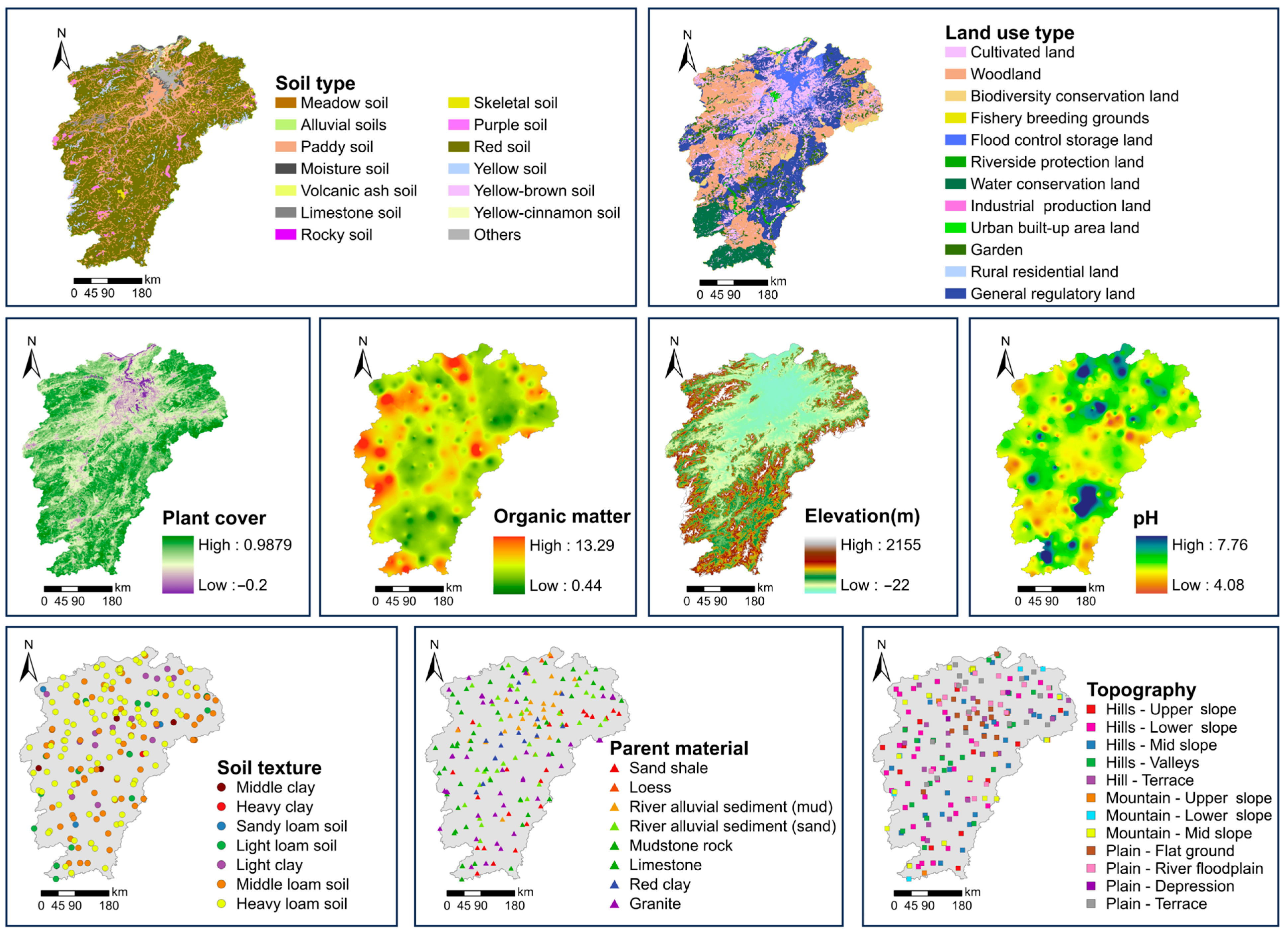
Nine environmental variables influencing soil element background concentrations were classified into two types (Figure 3): numerical type and categorical type. Descriptive statistics for the continuous numerical type variables, including altitude, pH, and organic matter, were presented in Table S1 from Supplementary Materials. The altitude in the study area ranged from 15.00 m to 1998.00 m, with a mean of 283.59 m, indicating substantial topographic variation. Soil pH ranged from 4.07 to 7.80, reflecting a slightly acidic to slightly alkaline condition across the study area. The organic matter varied between 0.43% and 13.49%, with an average of 4.01%, suggesting a moderate level of soil organic matter.
Six categorical type environmental variables were discrete, including soil type, parent material, plant cover, land use type, topography, and soil texture. The soil element background concentrations of heavy metals associated with these variables were summarized in Tables S2–S7. Limestone soil exhibited the highest average soil element background concentrations for most heavy metals, including Zn, Ni, Cr, Co, V, and Mn (Table S2). With respect to parent materials, the highest average background concentrations of Pb, Zn, Cd, Ni, Cr, and Mn were observed in limestone, while Cu, Co, and V reached their maxima in Xiashu loess (Table S3). In terms of plant cover, the highest background concentrations of Pb, As, Co, and Mn were found in wasteland, whereas Zn, Ni, and Cr were most elevated in areas covered by brush (Table S4). Regarding land use types, Cu, Ni, As, and Co showed the highest background concentrations in unused land, while Pb, Zn, and Mn had their highest values in grassland (Table S5). Among the topographical categories (plain, hill, and mountain), the highest average background concentrations of Pb, Hg, V, and Mn were observed on mountain upper slopes (Table S6). As for soil texture, Cr exhibited its maximum background concentrations in medium clay, while all other heavy metals, including Cu, Pb, Zn, Cd, Ni, Hg, As, Co, V, and Mn, showed the highest values in heavy clay soils (Table S7). These results indicated that categorical type environmental variables significantly influenced the background concentrations of various heavy metals in soil. However, as heavy metal concentrations were simultaneously affected by multiple environmental variables, the specific contribution of any single variable cannot be precisely determined based on univariate comparisons alone.
To further quantify the influence of individual categorical type environmental variables on the background concentrations of heavy metals, the Kruskal–Wallis (K–W) test was employed to assess the significance of differences in background concentrations across categories of each variable. A p-value less than 0.05 was considered indicative of a statistically significant effect. The distribution patterns of various heavy metals under different categorical type variables are summarized in Table S8. Significant differences in background concentrations among soil types were observed for all heavy metals except Co and Cu. For land use types, all heavy metals except Co, Cr, and Zn showed significant variation. In terms of plant cover, significant differences were found for all heavy metals except Cr, Mn, and Zn. With respect to topography, the background concentrations of As, Cd, Hg, Mn, Ni, and Pb exhibited significant variation across different terrain types. Similarly, all heavy metals except Co and Mn showed significant differences among different parent materials. Lastly, Co, Cr, Cu, Ni, and V displayed significant differences across soil texture categories. These results demonstrated that categorical type environmental variables exerted statistically significant influences on the background concentrations of specific heavy metals. However, the extent of their individual contributions still required multivariate analysis, given the potential interactions among variables.

3.1.2. Importance of Environmental Variables for Predicted Results

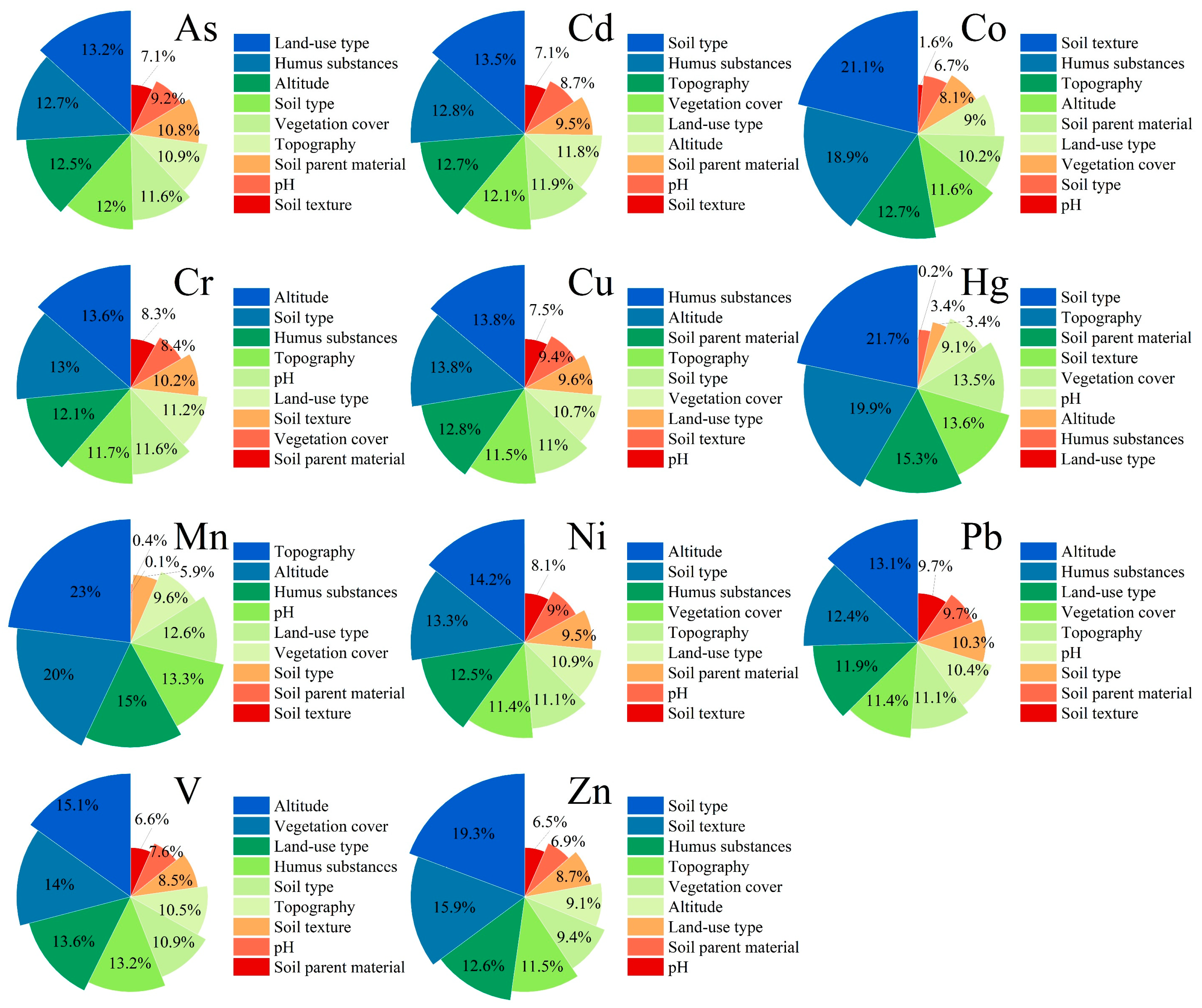
Given the significant influence of environmental variables on heavy metal concentrations, PCA and MLR were employed to identify the most relevant input variables for subsequent machine learning modeling. PCA and MLR were used to quantify the contribution of multiple environmental variables, including land use type, organic matter, altitude, soil type, plant cover, topography, parent material, pH, and soil texture, to the background concentrations of heavy metals. Environmental variables associated with principal components whose cumulative explained variance exceeded 90% were considered the dominant factors affecting background concentrations of heavy metals in the soil environment. The feature selection results from MLR were summarized in the Table S9. The contributions of nine environmental variables to the background concentrations of multiple heavy metals were presented in Figure 4. Notably, PCA selects a larger set of modeling indicators compared to MLR. Furthermore, PCA effectively eliminates inter-feature correlations, thus circumventing multicollinearity issues in the model. Therefore, these dominant variables identified by PCA were subsequently selected as input features for the predictive modeling.
Among these variables, soil type and organic matter exerted the greatest influence on the background concentrations of Cd, As, and Zn. Specifically, the background concentration of Cd was primarily influenced by soil type (13.5%), organic matter (12.8%), topography (12.7%), and plant cover (12.1%). For As, the most influential factors were land use type (13.2%), organic matter (12.7%), altitude (12.5%), and soil type (12.0%). Zn was mainly affected by soil type (19.3%), soil texture (15.9%), organic matter (12.6%), and topography (11.5%). Organic matter and altitude emerged as key factors influencing the background concentrations of Cu, Cr, Ni, Co, and Mn. For Cu, the major contributors were organic matter (13.8%), altitude (13.8%), parent material (12.8%), and topography (11.5%). Cr concentrations were primarily driven by altitude (13.6%), soil type (13.0%), organic matter (12.1%), and topography (11.7%). The background concentration of Ni was influenced most by altitude (14.2%), soil type (13.3%), organic matter (12.5%), and plant cover (11.4%). For Co, the dominant influencing variables were soil texture (21.1%), organic matter (18.9%), topography (12.7%), and altitude (11.6%). In the case of Mn, topography was the most influential factor (23.0%), followed by altitude (20.0%), organic matter (15.0%), and pH (13.3%). The most significant environmental variables influencing Pb concentrations were altitude (13.1%), organic matter (12.4%), land use type (11.9%), and plant cover (11.4%). A similar pattern was observed for V, with altitude (15.1%), plant cover (14.0%), land use type (13.6%), and organic matter (13.2%) being the dominant factors. In contrast to other heavy metals, Hg concentrations were primarily influenced by soil type (21.7%), topography (19.9%), parent material (15.3%), and soil texture (13.6%), indicating a distinct set of controlling variables for Hg. These findings underscore the critical roles of organic matter, topography, altitude, soil type, plant cover, and land use type as the significant environmental factors governing the background concentrations of heavy metals in soils.
Organic matter was identified as a key environmental variable influencing Cu concentrations. Organic matter formed metal–organic complexes with Cu ions through complexation, chelation, and adsorption reactions, thereby modulating their mobility and transformation in soil [41]. Topography was a significant determinant of Mn distribution. Topographic features affected soil formation and development by influencing runoff, drainage, and erosion processes [42], which in turn impacted the concentration and bioavailability of Mn. Altitude played a significant role in the accumulation of Cr, Ni, Pb, and V. In high-altitude regions, lower temperatures and higher precipitation levels enhanced atmospheric wet deposition through the “cold trapping” effect, promoting the accumulation of Cr, Ni, Pb, and V in soil [43]. Soil type strongly influenced the distribution of Cd, Zn, and Hg. Variations in parent material and pedogenesis significantly affected Cd, Zn, and Hg. Moreover, soil pH and organic matter were critical physicochemical properties governing metal mobility and retention [44]. Land use type emerged as a primary factor influencing the distribution of As. As a composite indicator of anthropogenic disturbances, changes in land use intensity and pattern had a direct impact on the spatial distribution of As [45,46]. Soil texture was the dominant factor affecting Co concentrations. Soils of different textures will adsorb Co to varying degrees, thus resulting in a higher Co content in heavy clay [47].

3.2. Comparison of Model Performance

3.2.1. Model Performance Evaluation

Following the filtering of environmental variables based on PCA-derived variance contributions, four machine learning algorithms, DT, XGBoost, RF, and SVM, were employed to predict the background concentrations of eleven heavy metals. Each model was run under two conditions: using the full set of variables (unfiltered input) and using the PCA-filtered subset of variables. This resulted in eight predictive scenarios: UNS-DT, UNS-XGBoost, UNS-RF, UNS-SVM, PCA-DT, PCA-XGBoost, PCA-RF, and PCA-SVM.
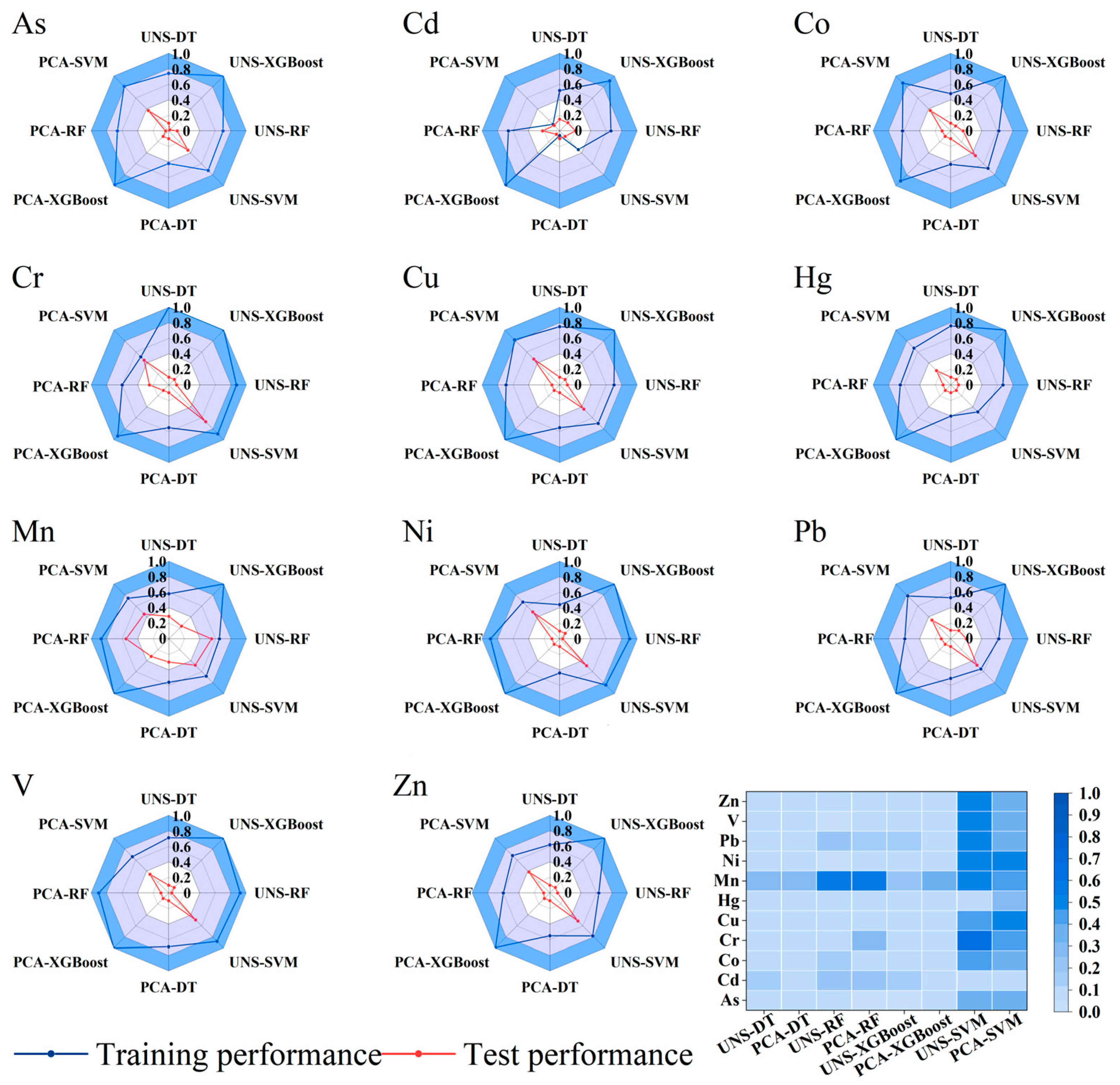
The R2, RMSE, and MAE were applied to evaluate the predictive accuracy of eight predictive scenarios, and the prediction performance of these scenarios based on R2 was illustrated in Figure 5. The results revealed that there were significant differences in the prediction performance among different combinations of machine learning and filtered environmental variables. For all heavy metals, the XGBoost model exhibited significant overfitting, characterized by excellent performance on the training set but markedly poor performance on the test set. Specifically, the training R2 of Cu, Hg, Ni, and V under the UNS-XGBoost and PCA-XGBoost models reached 1, while the test R2 was only 0.1. This issue was particularly pronounced due to the XGBoost model’s numerous hyperparameters and the unsuitability for the limited sample size, as also noted by Li et al. [48].
With the exception of Cd and Mn, the SVM model exhibited the best performance in training and testing across all heavy metals. The test R2 and train R2 of UNS-SVM for Cr reached 0.89 and 0.67, indicating high accuracy. At the same time, for Zn prediction, UNS-SVM achieved test and train R2 values of 0.78 and 0.51, indicating moderate accuracy. Notably, the test R2 for Cd (0.1) and Hg (0.1) of UNS-SVM was consistently low across all models. This indicated that the SVM model failed to fully compensate for the relationship between the background value concentrations of Cu and Hg and environmental variables.
In comparison, the RF model demonstrated a lower predictive accuracy than the SVM model and exhibited overfitting issues similar to the XGBoost model. The PCA-RF model showed poor performance for As, Co, Cr, Cu, Hg, Ni, Pb, V, and Zn, with test R2 values as low as 0.04, 0.11, 0.25, 0.1, 0.1, 0.1, 0.12, 0.1, and 0.08, respectively. Notably, for Ni and V, PCA-RF achieved high training R2 values (0.9) but significantly lower test R2 (0.1), further indicating severe overfitting. It was worth noting that the RF model achieved the optimal performance for Cd and Mn in both training and testing datasets compared with other models. The test R2 of the DT model was just 0.1–0.3, suggesting that the generalization ability of the DT model was relatively low.
Except for R2, the RMSE and MAE values of each heavy metal in eight scenarios were also used to identify the optimal model of each heavy metal, which was consistent with the analysis results of R2. Overall, the SVM model outperformed DT, XGBoost, and RF in terms of generalization ability, making it the most effective algorithm for predicting the background concentrations of heavy metals in this study.
Two predefined variable selection strategies, UNS and PCA, were found to influence the predictive performance of the machine learning models significantly. For instance, the optimal training model for Cr (test R2 = 0.65) was UNS-SVM, whereas PCA-SVM yielded poor performance for Cr (test R2 = 0.45). In the case of Cr, nine environmental variables (excluding parent material) contributed relatively evenly to the prediction. In contrast, the optimal training model for Mn (test R2 = 0.55) was UNS-RF and PCA-RF. The nine environmental variables exhibited substantially different influences on Mn background values, with topography contributing up to 23% of the variation, while parent material (0.1%) and soil texture (0.4%) showed minimal effects, respectively. This demonstrated that the influence of the input environmental variables of the model on the prediction accuracy of the model does not entirely depend on the removal of redundant variables.

3.2.2. Prediction Accuracy of Heavy Metals in Soil

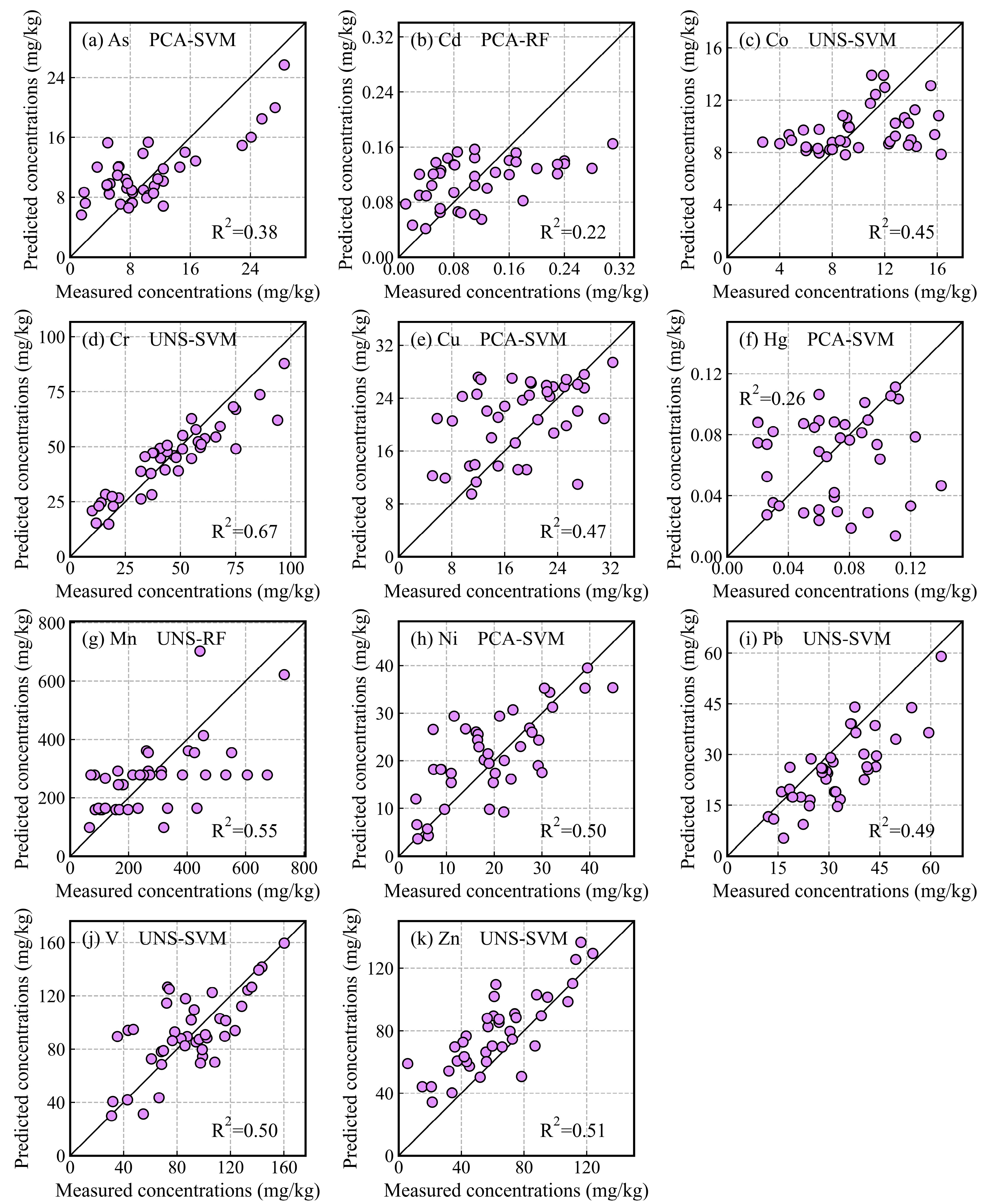
The relationship between the predicted and measured values under optimal model scenarios was illustrated in Figure 6. For most heavy metals, including Co, Cr, Cu, Mn, Ni, Pb, V, and Zn, the predicted concentrations closely matched the measured concentrations, indicating strong model performance. In contrast, noticeable deviations were observed for Cd and Hg. Accordingly, the R2 values of optimal models followed the descending order of Cr (0.67) > Mn (0.55) > Zn (0.51) > V (0.50) > Ni (0.50) > Pb (0.49) > Cu (0.47) > Co (0.45) > As (0.38) > Hg (0.26) > Cd (0.22) (Figure 5). The prediction accuracy of the machine learning model was influenced by the variability of the datasets, as reflected in the wide concentration ranges and standard deviation [40]. The high standard deviations of Cr (22.50) and Mn (179.12) contributed to superior predictive performance, whereas the low standard deviations of Hg (0.04) and Cd (0.07) resulted in poor prediction accuracy.
In addition to the influence of the original dataset quality, the intrinsic characteristics of the models also played a crucial role in determining predictive accuracy. The optimal prediction scenarios for As, Cu, Hg, and Ni were achieved using the PCA–SVM model, whereas those for Co, Cr, Pb, V, and Zn were best captured by the UNS–SVM model. Moreover, the PCA–RF model demonstrated the best performance for Cd concentration, while the UNS–RF model performed optimally for Mn. The superior fitting capability of the SVM model for As, Cu, Hg, Ni, Co, Cr, Pb, V, and Zn could be attributed to its ensemble-based architecture, which enabled it to manage small-sample, high-dimensional data effectively. Furthermore, SVM was well suited for modeling nonlinear relationships between heavy metal concentrations and environmental variables, particularly when enhanced by gradient-based optimization techniques [49]. Although the predictive power of the RF model was generally lower than that of XGBoost, it outperformed XGBoost in predicting Cd and Mn concentrations. Unlike other heavy metals, Cd and Mn exhibited a relatively large number of extreme value, including 14 and 11 samples, respectively, indicating that the spatial heterogeneity of Cd and Mn was very large. The RF model, which integrated predictions through either weighted averaging or majority voting, demonstrated strong robustness in noise filtering and extreme value processing [40,50]. This observation was consistent with the findings of Wu and Huang (2025) [17], who reported that RF outperformed XGBoost in predicting the natural background levels of Cd in soil.
The heavy metals, including As, Cu, Hg, Ni, and Cd, demonstrated improved predictive accuracy when environmental variables were filtered prior to modeling with the optimal machine learning algorithms. In contrast, Co, Cr, Pb, V, Zn, and Mn exhibited better predictive performance when all environmental variables were included. However, for the same heavy metal, the impact of variable filtering varied across different machine learning algorithms. For instance, Cr prediction using the UNS–SVM model outperformed the PCA–SVM model, while the PCA–RF model performed better than the UNS–RF model. These results indicated that filtering input variables did not universally enhance model accuracy. On the contrary, selecting “preferred” input features may not necessarily improve model performance and may even result in the loss of important information, thereby reducing predictive accuracy. This was because redundant variables identified by statistical correlation-based feature selection methods are only suggestive and not definitive [51].

3.3. Regional Comparisons of SBGs: Validation of Predictive Results

The spatial distribution maps of measured and predicted heavy metal concentrations generated by the optimal models are presented in Figure 7. Among all heavy metals, Cr exhibited the highest prediction accuracy, with both measured and predicted concentrations consistently showing elevated values in the western part of the study area and lower values in the east. The predictive performance for As, Co, Cu, Mn, Ni, Pb, and V was also relatively good. The predictive models reproduced the spatial distribution trends of these heavy metals, although some systematic biases were observed. For instance, the predicted concentrations of As and Ni tended to be overestimated at low concentrations and slightly underestimated at high concentrations. In the case of Co, the predicted concentrations were notably higher than the measured values in the eastern and northern regions. For Mn, localized discrepancies were evident, particularly in the southeastern part of the study area, where the predicted values did not align well with the measured concentrations.
The predictive performance for Cd and Hg was unsatisfactory. Compared to the measured concentrations, the model substantially overestimated Cd levels in the southern parts and underestimated them in the northern parts. For Hg, the predicted spatial distribution deviated significantly from the measured values, indicating a poor match. These results suggested that while the model effectively captured the overall spatial patterns for most heavy metals, it required further refinement to reduce prediction biases for specific elements. In particular, the prediction of Cd and Hg may necessitate fundamental improvements in the modeling strategy to enhance accuracy.

3.4. Advantages, Limitations and Future Research Perspectives

This study utilizes soil element background concentration data from 1987 to 1988, as it better represents pre-anthropogenic conditions. To address the high costs associated with province-wide background value determination, this study innovatively proposes a prediction framework: establishing a model based on historical environmental variables and historical background concentrations, then applying it to predict values for other uncontaminated periods. This approach eliminates the need for large-scale sampling by relying solely on routine monitoring data, significantly reducing costs. Prediction accuracy can be further enhanced through small-scale sampling calibration, offering an efficient and economical, technical solution for regional environmental research.
The core advantage of machine learning algorithms in predicting soil environmental background values lies in their ability to parse complex nonlinear relationships and integrate high-dimensional data. Traditional statistical methods are limited by preset distribution assumptions and simple covariate relationships. In contrast, algorithms such as decision trees, random forests, XGBoost, and support vector machines can precisely capture the interaction between soil heavy metal background value content and multiple environmental factors (e.g., topography, parent material, and plant cover) by constructing multi-layered decision rules or hidden layer transformations. This nonlinear modeling capability significantly enhances the prediction accuracy of background values in regions with strong spatial heterogeneity, especially addressing the systematic bias of traditional methods at the edges of mineralized zones or in complex geomorphic areas. Moreover, the adaptive optimization mechanisms of these algorithms, such as weighted voting in ensemble learning and backpropagation in deep learning, endow the models with stronger generalization capabilities. Even in the face of regional data sparsity, key driving factors can be selected through feature importance analysis to reduce noise interference. Compared with previous research by Barkhordari and Qi [8], this study fully utilized the advantages of various machine learning models, identifying the most suitable machine learning algorithm for each heavy metal. Among all predicted heavy metals, the RF model achieved the best prediction results for Cd and Mn, while the SVM model demonstrated optimal predictive performance for the remaining heavy metals. Compared with existing research by Wu et al. [17], this study enabled the production of spatially continuous, high-resolution distribution maps of element background values, confirming the robustness and reliability of the model predictions. The optimal models effectively predicted spatial distributions for most heavy metals (Cr, As, Co, Cu, Mn, Ni, Pb, V) but showed systematic biases for Cd and Hg, requiring model refinement for these heavy metals.
Although demonstrating exceptional predictive performance, machine learning algorithms still exhibit certain limitations in the process of model construction and practical application. Firstly, the data dependency risk of machine learning algorithms is prominent. Model prediction accuracy is highly contingent upon the representativeness and quality of the training samples. The dataset used in the case study was relatively small and unevenly distributed, which may be insufficient to capture the complex distribution patterns of soil elements comprehensively and cannot provide a solid learning foundation for machine learning algorithms. As a result, this contributed to suboptimal learning accuracy and elevated generalization errors in the decision tree and XGBoost models. Therefore, it is necessary to expand the dataset to provide diverse and representative data information, bolster the stability and reliability of the model, particularly for the prediction of soil environmental background values in regions characterized by high spatial heterogeneity. Secondly, the selection of environmental variables affects the prediction performance of the model. Appropriate input features are crucial for constructing effective, accurate, and reliable prediction models. Further broadening the types and scope of environmental variables and identifying those significantly influencing soil environmental background values would enable a more precise delineation of the complex nonlinear relationships between background values and environmental factors. Additionally, while this case study revealed that distinct optimal models were required for different elements, the inherent black-box nature of these models necessitates enhanced interpretability for the selected model corresponding to each element. Future work should refine the optimization and selection of optimal predictive models for soil elemental background values by incorporating scale-specific, data type-specific, and element type-specific considerations, building upon the distinct characteristics of different machine learning algorithms.
The machine learning model developed in this study for predicting soil element background concentrations has certain practical value and is expected to be integrated into the national soil environmental quality monitoring system. It is expected to provide technical support in three key areas of environmental management: (1) the high-resolution spatial maps of background concentrations generated by the model can be used to conduct multi-time-scale and multi-spatial dimension comparisons between historical baselines and current monitoring data, thereby offering references for assessing the evolution of soil environmental quality; (2) the proposed prediction framework can be used to establish a low-cost, province-scale estimation protocol based on environmental covariates, thus addressing the high sampling cost associated with conventional methods; and (3) for target elements with larger prediction deviations, such as Cd and Hg, hybrid models incorporating auxiliary features (e.g., geological accumulation indices) can be developed, and their optimized results can serve as a quantitative basis for dynamic adjustment of heavy metal risk control values.

4. Conclusions

Based on the key factors as input variables, four ML models were used to predict the background concentrations of soil As, Cd, Co, Cr, Cu, Hg, Mn, Ni, Pb, V, and Zn at a large regional scale. To achieve good modeling results, several optimization algorithm methods were evaluated in terms of their performance. Among all the models evaluated, the SVM model exhibited the best prediction performance with highest R2 values reaching 0.67, substantially higher than those achieved by other models (R2 = 0.22–0.55). Variable importance analysis revealed soil type as the predominant predictor of background concentrations for Cd, Hg, and Zn, while altitude dominated the spatial variation in Cr, Ni, Pb, and V. Land use type, soil texture, organic matter content, and topography were identified as the key determinants for As, Co, Cu, and Mn distributions, respectively. Collectively, organic matter, topography, altitude, and soil type emerged as statistically significant drivers of soil element spatial patterns, explaining >60% of total variability in the dataset. By selecting suitable algorithms and optimizing input variables, this study successfully and effectively predicted the background concentrations of soil heavy metals. These results confirm that the modeling of background values in soil environments is a nonlinear problem. The prediction results can provide decision support for assessing and diagnosing the contamination of heavy metals in agricultural soil.
This study developed a soil environmental background value prediction model based on machine learning algorithms, demonstrating significant potential in environmental pollution prevention and control, farmland environmental safety management, and sustainable land resource utilization. Firstly, the high-precision spatial distribution maps of soil environmental background values generated by the model can accurately distinguish between natural background and anthropogenic pollution, thereby avoiding the misjudgment of high-background-value areas as polluted areas for excessive treatment. At the same time, for areas where on-site data is scarce or difficult to obtain, the prediction of soil environmental background values is achieved through multi-source data-driven methods, effectively reducing monitoring costs and supporting precise policy making by environmental regulatory authorities. Secondly, these spatial distribution maps support differentiated fertilization by quantifying the natural abundance and deficiency patterns of soil elements, assessing the baseline state of farmland soil health for early degradation warnings, and identifying soil pollution sources in cultivated land to guide the delineation of control zones and adjustments in crop layout, thereby facilitating smart agriculture and safe planting. Finally, these in situ soil environmental background value data can provide a scientific basis for sustainable land resource planning, including identifying ecologically sensitive areas, tracing historical pollution trajectories to clarify responsibility, and formulating site-specific remediation goals. Taken together, this study provides a practical and scalable framework for predicting soil element background concentrations, offering robust technical support for environmental monitoring, regulatory standard development, and dynamic risk management.

Supplementary Materials

The following supporting information can be downloaded at https://www.mdpi.com/article/10.3390/su17177853/s1. Table S1: The descriptive statistics of altitude, pH and organic matter; Table S2: The average natural background levels of heavy metals in different soil types; Table S3: The average natural background levels of heavy metals in different parent materials; Table S4: The average natural background levels of heavy metals in different plant covers; Table S5: The average natural background levels of heavy metals in different land use types; Table S6: The average natural background levels of heavy metals in different topographies; Table S7: The average natural background levels of heavy metals in different soil textures; Table S8: The differentiation law of heavy metal concentrations among different environmental variable units; Table S9: The screening results of multiple linear regression.

Author Contributions

Conceptualization, J.L. and P.X.; methodology, L.M. and H.W.; software, T.L.; validation, L.M.; data curation, J.L.; writing—original draft, J.L.; writing—review and editing, J.L. and J.H.; visualization, J.L.; supervision, P.X. and H.W.; funding acquisition, J.L. All authors have read and agreed to the published version of the manuscript.

Funding

This research was funded by the Youth Science and Technology Innovation Fund Project of the Technical Centre for Soil, Agriculture and Rural Ecology and Environment, Ministry of Ecology and Environment (QKC20220001).

Institutional Review Board Statement

Not applicable.

Informed Consent Statement

Not applicable.

Data Availability Statement

The dataset is available on request from the authors.

Conflicts of Interest

The authors declare no conflicts of interest.

Abbreviations

The following abbreviations are used in this manuscript:
DTDecision tree
RFRandom forest
XGBoostExtreme gradient boosting
SVMSupport vector machine
MLMachine learning
AsArsenic
CdCadmium
CoCobalt
CrChromium
CuCopper
HgMercury
MnManganese
NiNickel
PbLead
VVanadium
ZnZinc
GLMGeneral linear models
DDTCDiethyldithiocabamate
UNSUnfiltered input
PCAPrincipal component analysis
KMOKaiser–Meyer–Olkin
MLRMultiple linear regression
R2The coefficient of determination
RMSERoot mean squared error
MAEMean absolute error
K–WKruskal–Wallis

References

  1. Silva, F.L.; Martins E Silva, M.H.; Veiga, J.B.; Silva, A.C.S.; Carvalho, M.A.C.; Weber, O.L.S.; Eguchi, E.S.; López-Alonso, M.; Oliveira-Júnior, E.S.; Guilherme, L.R.G.; et al. Assessing Background Levels of Trace Elements in Soils of Mato Grosso (Brazil) for Environmental and Food Security. Catena 2024, 244, 108267. [Google Scholar] [CrossRef]
  2. Amiri, V.; Sohrabi, N.; Lak, R.; Tajbakhsh, G. Estimation of Natural Background Levels of Heavy Metals and Major Variables in Groundwater to Ensure the Sustainable Supply of Safe Drinking Water in Fereidan, Iran. Environ. Dev. Sustain. 2023, 26, 19807–19832. [Google Scholar] [CrossRef]
  3. Sulieman, M.M.; Kaya, F.; Keshavarzi, A.; Hussein, A.M.; Al-Farraj, A.S.; Brevik, E.C. Spatial Variability of Some Heavy Metals in Arid Harrats Soils: Combining Machine Learning Algorithms and Synthetic Indexes Based-Multitemporal Landsat 8/9 to Establish Background Levels. Catena 2024, 234, 107579. [Google Scholar] [CrossRef]
  4. Meloni, F.; Nisi, B.; Gozzi, C.; Rimondi, V.; Cabassi, J.; Montegrossi, G.; Rappuoli, D.; Vaselli, O. Background and Geochemical Baseline Values of Chalcophile and Siderophile Elements in Soils around the Former Mining Area of Abbadia San Salvatore (Mt. Amiata, Southern Tuscany, Italy). J. Geochem. Explor. 2023, 255, 107324. [Google Scholar] [CrossRef]
  5. Zhang, X.; Deng, W.; Yang, X. The Background Concentrations of 13 Soil Trace Elements and Their Relationships to Parent Materials and Vegetation in Xizang (Tibet), China. J. Asian Earth Sci. 2002, 21, 167–174. [Google Scholar] [CrossRef]
  6. Mascarenhas, R.B.; Gloaguen, T.V.; Hadlich, G.M.; Gomes, N.S.; Almeida, M.D.C.; Souza, E.D.S.; Bomfim, M.R.; Costa, O.D.V.; Gonzaga Santos, J.A. The Challenge of Establishing Natural Geochemical Backgrounds in Human-Impacted Mangrove Soils of Northeastern Brazil. Chemosphere 2025, 376, 144261. [Google Scholar] [CrossRef] [PubMed]
  7. Xia, X.; Ji, J.; Zhang, C.; Yang, Z.; Shi, H. Carbonate Bedrock Control of Soil Cd Background in Southwestern China: Its Extent and Influencing Factors Based on Spatial Analysis. Chemosphere 2022, 290, 133390. [Google Scholar] [CrossRef]
  8. Barkhordari, M.S.; Qi, C. Prediction of Soil Arsenic Concentration in European Soils: A Dimensionality Reduction and Ensemble Learning Approach. J. Hazard. Mater. Adv. 2025, 17, 100604. [Google Scholar] [CrossRef]
  9. Zeng, W.; Wan, X.; Lei, M.; Gu, G.; Chen, T. Influencing Factors and Prediction of Arsenic Concentration in Pteris Vittata: A Combination of Geodetector and Empirical Models. Environ. Pollut. 2022, 292, 118240. [Google Scholar] [CrossRef]
  10. Zhang, Z.; Lu, Y.; Li, L.; Zeng, F.; Li, X.; Li, L.; Yue, J. Elevational Patterns in the Diversity and Composition of Soil Archaeal and Bacterial Communities Depend on Climate, Vegetation, and Soil Properties in an Arid Mountain Ecosystem. Catena 2025, 249, 108679. [Google Scholar] [CrossRef]
  11. Kirkpatrick, J.B.; Green, K.; Bridle, K.L.; Venn, S.E. Patterns of Variation in Australian Alpine Soils and Their Relationships to Parent Material, Vegetation Formation, Climate and Topography. Catena 2014, 121, 186–194. [Google Scholar] [CrossRef]
  12. More, S.; Dhakate, R. Geogenic and Anthropogenic Sources of Heavy Metals in Soil: An Ecological and Health Risk Assessment in the Granitic Terrain of South India. Catena 2025, 254, 108960. [Google Scholar] [CrossRef]
  13. Gałązka, A.; Marzec-Grządziel, A.; Grządziel, J.; Varsadiya, M.; Pawlik, Ł. Fungal Genetic Biodiversity and Metabolic Activity as an Indicator of Potential Biological Weathering and Soil Formation—Case Study of towards a Better Understanding of Earth System Dynamics. Ecol. Indic. 2022, 141, 109136. [Google Scholar] [CrossRef]
  14. Adhikari, K.; Mancini, M.; Libohova, Z.; Blackstock, J.; Winzeler, E.; Smith, D.R.; Owens, P.R.; Silva, S.H.G.; Curi, N. Heavy Metals Concentration in Soils across the Conterminous USA: Spatial Prediction, Model Uncertainty, and Influencing Factors. Sci. Total Environ. 2024, 919, 170972. [Google Scholar] [CrossRef]
  15. Ma, X.; Wang, J.; Zhou, K.; Zhang, W.; Chen, A. Uncertainty in Soil Elemental Prediction Using Machine Learning and Hyperspectral Remote Sensing. J. Hazard. Mater. 2025, 494, 138502. [Google Scholar] [CrossRef]
  16. Proshad, R.; Asharaful Abedin Asha, S.M.; Tan, R.; Lu, Y.; Abedin, M.A.; Ding, Z.; Zhang, S.; Li, Z.; Chen, G.; Zhao, Z. Machine Learning Models with Innovative Outlier Detection Techniques for Predicting Heavy Metal Contamination in Soils. J. Hazard. Mater. 2025, 481, 136536. [Google Scholar] [CrossRef]
  17. Wu, J.; Huang, C. Machine Learning-Supported Determination for Site-Specific Natural Background Values of Soil Heavy Metals. J. Hazard. Mater. 2025, 487, 137276. [Google Scholar] [CrossRef]
  18. Li, W.; Huang, G.; Tang, N.; Lu, P.; Jiang, L.; Lv, J.; Qin, Y.; Lin, Y.; Xu, F.; Lei, D. Effects of Heavy Metal Exposure on Hypertension: A Machine Learning Modeling Approach. Chemosphere 2023, 337, 139435. [Google Scholar] [CrossRef]
  19. Ma, X.; Guan, D.-X.; Zhang, C.; Yu, T.; Li, C.; Wu, Z.; Li, B.; Geng, W.; Wu, T.; Yang, Z. Improved Mapping of Heavy Metals in Agricultural Soils Using Machine Learning Augmented with Spatial Regionalization Indices. J. Hazard. Mater. 2024, 478, 135407. [Google Scholar] [CrossRef]
  20. Yan, Y.; Yang, Y. Revealing the Synergistic Spatial Effects in Soil Heavy Metal Pollution with Explainable Machine Learning Models. J. Hazard. Mater. 2025, 482, 136578. [Google Scholar] [CrossRef] [PubMed]
  21. Barkhordari, M.S.; Qi, C. Prediction of Zinc, Cadmium, and Arsenic in European Soils Using Multi-End Machine Learning Models. J. Hazard. Mater. 2025, 490, 137800. [Google Scholar] [CrossRef]
  22. Zhang, B.; Hou, H.; Huang, Z.; Zhao, L. Estimation of Heavy Metal Soil Contamination Distribution, Hazard Probability, and Population at Risk by Machine Learning Prediction Modeling in Guangxi, China. Environ. Pollut. 2023, 330, 121607. [Google Scholar] [CrossRef]
  23. Zhang, K.; Wang, X.; Liu, T.; Wei, W.; Zhang, F.; Huang, M.; Liu, H. Enhancing Water Quality Prediction with Advanced Machine Learning Techniques: An Extreme Gradient Boosting Model Based on Long Short-Term Memory and Autoencoder. J. Hydrol. 2024, 644, 132115. [Google Scholar] [CrossRef]
  24. He, J.L.; Xu, G.Y.; Zhu, H.M.; Peng, G.H. Study on Soil Enrionmental Background Values in Jiangxi Province; China Environmental Science Press: Beijing, China, 2006. [Google Scholar]
  25. Hartemink, A.E.; Bockheim, J.G. Soil Genesis and Classification. Catena 2013, 104, 251–256. [Google Scholar] [CrossRef]
  26. Xu, Y.; Li, P.; Zhang, Z.; Gu, Y.; Xiao, L.; Liu, X.; Wang, B. Integrating Machine Learning for Enhanced Spatial Prediction and Risk Assessment of Soil Heavy Metal(Loid)s. Environ. Pollut. 2025, 383, 126919. [Google Scholar] [CrossRef]
  27. Rostami, A.A.; Sedghi, Z.; Nadiri, A.A.; Barzegar, R.; Dimova, N.T.; Senapathi, V.; Islam, A.R.M.T. Harnessing Deep Learning for Fusion-Based Heavy Metal Contamination Index Prediction in Groundwater. J. Contam. Hydrol. 2025, 274, 104672. [Google Scholar] [CrossRef]
  28. Quinlan, J.R. Induction of Decision Trees. Mach. Learn. 1986, 1, 81–106. [Google Scholar] [CrossRef]
  29. Breiman, L.; Friedman, J.H.; Olshen, R.A.; Stone, C.J. Classification and Regression Trees, 1st ed.; Routledge: London, UK, 2017; ISBN 978-1-315-13947-0. [Google Scholar]
  30. Breiman, L. Random Forests. Mach. Learn. 2001, 45, 5–32. [Google Scholar] [CrossRef]
  31. Chen, D.; Wang, X.; Luo, X.; Huang, G.; Tian, Z.; Li, W.; Liu, F. Delineating and Identifying Risk Zones of Soil Heavy Metal Pollution in an Industrialized Region Using Machine Learning. Environ. Pollut. 2023, 318, 120932. [Google Scholar] [CrossRef]
  32. Zhang, H.; Yin, A.; Yang, X.; Fan, M.; Shao, S.; Wu, J.; Wu, P.; Zhang, M.; Gao, C. Use of Machine-Learning and Receptor Models for Prediction and Source Apportionment of Heavy Metals in Coastal Reclaimed Soils. Ecol. Indic. 2021, 122, 107233. [Google Scholar] [CrossRef]
  33. Friedman, J.H. Stochastic Gradient Boosting. Comput. Stat. Data Anal. 2002, 38, 367–378. [Google Scholar] [CrossRef]
  34. Suleymanov, A.; Suleymanov, R.; Kulagin, A.; Yurkevich, M. Mercury Prediction in Urban Soils by Remote Sensing and Relief Data Using Machine Learning Techniques. Remote Sens. 2023, 15, 3158. [Google Scholar] [CrossRef]
  35. Chen, T.; Guestrin, C. XGBoost: A Scalable Tree Boosting System. In Proceedings of the 22nd ACM SIGKDD International Conference on Knowledge Discovery and Data Mining, San Francisco, CA, USA, 13 August 2016; pp. 785–794. [Google Scholar]
  36. Cortes, C.; Vapnik, V. Support-Vector Networks. Mach. Learn. 1995, 20, 273–297. [Google Scholar] [CrossRef]
  37. Vapnik, V.N. Statistical Learning Theory (Adaptive and Learning Systems for Signal Processing, Communications, and Control); Wiley: New York, NY, USA, 1998; ISBN 978-0-471-03003-4. [Google Scholar]
  38. Park, Y.; Cho, K.H.; Park, J.; Cha, S.M.; Kim, J.H. Development of Early-Warning Protocol for Predicting Chlorophyll-a Concentration Using Machine Learning Models in Freshwater and Estuarine Reservoirs, Korea. Sci. Total Environ. 2015, 502, 31–41. [Google Scholar] [CrossRef] [PubMed]
  39. Varley, A.; Tyler, A.; Smith, L.; Dale, P.; Davies, M. Remediating Radium Contaminated Legacy Sites: Advances Made through Machine Learning in Routine Monitoring of “Hot” Particles. Sci. Total Environ. 2015, 521, 270–279. [Google Scholar] [CrossRef] [PubMed]
  40. Li, K.; Guo, G.; Zhang, D.; Lei, M.; Wang, Y. Accurate prediction of spatial distribution of soil potentially toxic elements using machine learning and associated key influencing factors identification: A case study in mining and smelting area in southwestern China. J. Hazard. Mater. 2024, 478, 135454. [Google Scholar] [CrossRef]
  41. Piccolo, A.; Spaccini, R.; De Martino, A.; Scognamiglio, F.; Di Meo, V. Soil Washing with Solutions of Humic Substances from Manure Compost Removes Heavy Metal Contaminants as a Function of Humic Molecular Composition. Chemosphere 2019, 225, 150–156. [Google Scholar] [CrossRef]
  42. Liu, H.; Xiong, Z.; Jiang, X.; Liu, G.; Liu, W. Heavy Metal Concentrations in Riparian Soils along the Han River, China: The Importance of Soil Properties, Topography and Upland Land Use. Ecol. Eng. 2016, 97, 545–552. [Google Scholar] [CrossRef]
  43. Blackwell, B.D.; Driscoll, C.T. Deposition of Mercury in Forests along a Montane Elevation Gradient. Environ. Sci. Technol. 2015, 49, 5363–5370. [Google Scholar] [CrossRef]
  44. Zhou, W.; Li, Z.; Liu, Y.; Shen, C.; Tang, H.; Huang, Y. Soil Type Data Provide New Methods and Insights for Heavy Metal Pollution Assessment and Driving Factors Analysis. J. Hazard. Mater. 2024, 480, 135868. [Google Scholar] [CrossRef]
  45. Wang, Z.; Xiao, J.; Wang, L.; Liang, T.; Guo, Q.; Guan, Y.; Rinklebe, J. Elucidating the Differentiation of Soil Heavy Metals under Different Land Uses with Geographically Weighted Regression and Self-Organizing Map. Environ. Pollut. 2020, 260, 114065. [Google Scholar] [CrossRef] [PubMed]
  46. Yaşar Korkanç, S.; Korkanç, M.; Amiri, A.F. Effects of Land Use/Cover Change on Heavy Metal Distribution of Soils in Wetlands and Ecological Risk Assessment. Sci. Total Environ. 2024, 923, 171603. [Google Scholar] [CrossRef]
  47. Zhong, X.; Chen, Z.; Li, Y.; Ding, K.; Liu, W.; Liu, Y.; Yuan, Y.; Zhang, M.; Baker, A.J.M.; Yang, W.; et al. Factors Influencing Heavy Metal Availability and Risk Assessment of Soils at Typical Metal Mines in Eastern China. J. Hazard. Mater. 2020, 400, 123289. [Google Scholar] [CrossRef]
  48. Li, C.; Yang, Z.; Guan, D.-X.; Yu, T.; Jiang, Z.; Wu, X.; Yang, Y.; Luan, S.; Xu, H.; Huang, C.; et al. Spatial-Machine Learning Framework for Rapid Identification of Soil Cadmium Risk in High Geochemical Background Areas. J. Hazard. Mater. 2025, 492, 138091. [Google Scholar] [CrossRef]
  49. Moradpour, S.; Entezari, M.; Ayoubi, S.; Karimi, A.; Naimi, S. Digital Exploration of Selected Heavy Metals Using Random Forest and a Set of Environmental Covariates at the Watershed Scale. J. Hazard. Mater. 2023, 455, 131609. [Google Scholar] [CrossRef]
  50. Feng, B.; Ma, J.; Liu, Y.; Wang, L.; Zhang, X.; Zhang, Y.; Zhao, J.; He, W.; Chen, Y.; Weng, L. Application of Machine Learning Approaches to Predict Ammonium Nitrogen Transport in Different Soil Types and Evaluate the Contribution of Control Factors. Ecotoxicol. Environ. Saf. 2024, 284, 116867. [Google Scholar] [CrossRef]
  51. Zhang, S.; Li, X.; Zong, M.; Zhu, X.; Cheng, D. Learning k for kNN Classification. ACM Trans. Intell. Syst. Technol. 2017, 8, 1–19. [Google Scholar] [CrossRef]
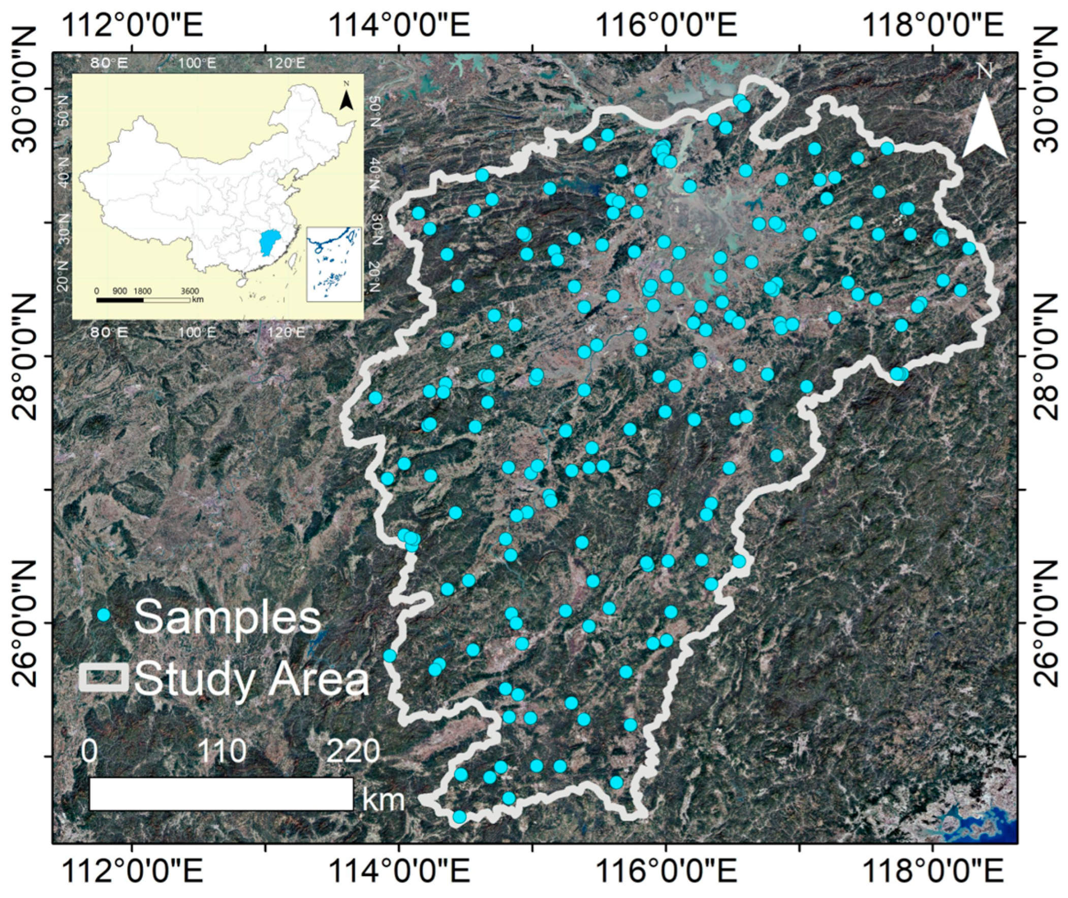
Figure 1. Map of the study area with locations for soil sampling.
Sustainability 17 07853 g001
Figure 2. The theoretical framework for predicting the soil element background concentration through machine learning.
Sustainability 17 07853 g002
Figure 3. The spatial distribution maps of nine environmental variables, including soil type, land use type, plant cover, organic matter, elevation, pH, soil texture, parent material, and topography.
Sustainability 17 07853 g003
Figure 4. Contribution of the environmental variables to heavy metals in soil by the PCA method.
Sustainability 17 07853 g004
Figure 5. The model simulation effects of 11 heavy metals in 8 scenarios represented by R2.
Sustainability 17 07853 g005
Figure 6. Comparison of the predicted values and measured values of each heavy metal simulated by the model under the optimal combination scenario.
Sustainability 17 07853 g006
Figure 7. Spatial distribution map of prediction results and measured values of background values of heavy metals in soil.
Sustainability 17 07853 g007
Table 1. Six scenarios for predicting natural concentrations of heavy metals in soil.
ML ModelIndicator Screening MethodScenario Settings
DTUNSScenario 1: UNS-D
PCAScenario 2: PCA-DT
RFUNSScenario 3: UNS-RF
PCAScenario 4: PCA-RF
XGBoostUNSScenario 5: UNS-XGBoost
PCAScenario 6: PCA-XGBoost
SVMUNSScenario 7: UNS-SVM
PCAScenario 8: PCA-SVM
Disclaimer/Publisher’s Note: The statements, opinions and data contained in all publications are solely those of the individual author(s) and contributor(s) and not of MDPI and/or the editor(s). MDPI and/or the editor(s) disclaim responsibility for any injury to people or property resulting from any ideas, methods, instructions or products referred to in the content.