Spatiotemporal Responses and Threshold Mechanisms of Urban Landscape Patterns to Ecosystem Service Supply–Demand Dynamics in Central Shenyang, China

Abstract

Clarifying the spatiotemporal relationship between urban ecosystem services and changes in landscape patterns is essential, as it has significant implications for balancing ecological protection with socio-economic development. However, existing studies have largely focused on the one-sided impact of landscape patterns on either the supply or demand of ESs, with limited investigation into how changes in these patterns affect the growth rates of both supply and demand. The central urban area, characterized by complex urban functions, intricate land use structures, and diverse environmental challenges, further complicates this relationship; yet, the spatiotemporal differentiation patterns of ecosystem services’ supply–demand dynamics in such regions, along with the underlying influencing mechanisms, remain insufficiently explored. To address this gap, the present study uses Shenyang’s central urban area, China as a case study, integrating multiple data sources to quantify the spatiotemporal variations in landscape pattern indices and five ecosystem services: water retention, flood regulation, air purification, carbon sequestration, and habitat quality. The XGBoost model is employed to construct non-linear relationships between landscape pattern indices and the supply–demand ratios of these services. Using SHAP values and LOWESS analysis, this study evaluates both the magnitude and direction of each landscape pattern index’s influence on the ecological supply–demand ratio. The findings outlined above indicate that: there are distinct disparities in the spatiotemporal distribution of landscape pattern indices at the patch type level. Additionally, the changing trends in the supply, demand, and supply–demand ratios of ecosystem services show spatiotemporal differentiation. Overall, the ecosystem services in the study area are developing negatively. Further, the impact of landscape pattern characteristics on ecosystem services is non-linear. Each index has a unique effect, and there are notable threshold intervals. This study provides a novel analytical approach for understanding the intricate relationship between landscape patterns and ESs, offering a scientific foundation and practical guidance for urban ecological protection, restoration initiatives, and territorial spatial planning.

1. Introduction

Human activities that alter the Earth’s surface can inflict irreversible damage on the delicate balance between regional natural ecosystems and socio-economic systems. Scientific spatial management plays a crucial role in optimizing ecosystem patterns and processes, thereby enhancing human well-being and promoting regional sustainability. Increasingly, scholars advocate for the integration of ecosystems into spatial management frameworks to effectively address urban ecological challenges and support sustainable urban development [1]. Ecosystem services (ESs) refer to the benefits that humans obtain, either directly or indirectly, from ecosystems and their functions [2], providing the material foundation and essential conditions necessary for human survival and development [3]. The supply of ESs represents the capacity of a specific area to generate these benefits, while demand denotes the total quantity of services consumed, utilized, or valued within a region over a defined time frame [4,5]. The interplay between the supply and demand of ESs constitutes a complex dynamic process, reflecting the transfer of benefits from natural ecosystems to economic and social systems. Gaining insight into the spatial and temporal variations in this supply–demand relationship is vital, as it offers valuable theoretical support for landscape ecological planning and informed spatial management.

As urbanization accelerates, the proliferation of high-density building clusters, expansive road networks, and the fragmentation of natural green spaces have significantly altered the structure and function of urban landscapes. These transformations have adversely impacted the urban natural environment and reduced the availability of ESs. Simultaneously, as urban residents experience improvements in both awareness and quality of life, the demand for ESs continues to rise. Data show that for every 10% increase in average household income, the demand for urban green spaces increases by 1% [6]. This growing imbalance between the supply and demand of ESs can diminish urban spatial efficiency and hinder the high-quality development of cities [7]. Therefore, identifying areas where the supply–demand relationship of ESs is progressing positively—along with determining their key influencing factors and optimal thresholds for encouraging such progress—is essential. Maintaining a consistent balance of ESs, promoting the orderly development of the complex human–land coupling system, and offering practical, generalizable strategies for harmonizing urban ecological development with economic and social growth are all vital. These efforts are crucial for achieving sustainable urban development and enhancing overall human well-being.

In China, as urban functions transition from production oriented to service oriented, integrating both quantitative and qualitative analyses of ESs and landscape patterns has become increasingly important [8,9,10]. This integration enables a deeper understanding of the spatiotemporal differentiation of ecosystems and helps address regional resource and environmental issues related to ecological processes. Urban landscape patterns are shaped by the complex interplay between natural systems and socio-ecological dynamics, reflecting the feedback mechanisms between human decisions and ecological functions [11,12]. Landscape pattern indices, widely used as indicators, effectively capture spatial variations and serve as indirect tools for assessing the ecological impacts of urbanization [13,14]. The dynamic relationship between landscape pattern metrics and the supply–demand dynamics of ESs represents a core research focus in both landscape ecology and ES science. This relationship is fundamentally characterized by a reciprocal feedback mechanism between landscape structure and ecological function: landscape patterns influence the supply capacity of ESs by shaping ecological structures and processes, while the equilibrium between ES supply and demand, in turn, drives anthropogenic landscape changes, thereby modifying landscape patterns once again [15]. This bidirectional interaction is co-regulated by temporal scales, spatial heterogeneity, and human activities. Understanding these interconnections is vital for providing theoretical support to resolve the long-standing paradox between ecological protection and human development, ultimately promoting sustainable landscape management and achieving a balanced state in ES supply and demand.

Numerous studies have demonstrated that optimizing landscape patterns can significantly enhance ESs. In terms of the research content, at the supply level, Ayinuer et al. investigated the relationship between ES values and landscape indices in the Ebinur Lake Basin [16] and found a significant positive correlation between landscape diversity indices and ES values. Similarly, Yang et al. analyzed the impact of landscape pattern changes on ES supply in Beijing, recommending an increase in forest and grassland areas at the landscape level and the expansion of average patch areas of croplands at the type level [13]. Zhang et al. identified high-efficiency ES synergistic zones in Fujian Province, China, using visual machine learning models. Their findings revealed that landscape pattern factors have optimal driving thresholds and sensitive regulation intervals for the Total ESs (TES) index. Notably, once the proportion of construction land exceeds 10%, further expansion does not significantly amplify its negative impact on TES [17]. On the demand side, existing research primarily focuses on improving demand conditions through the regulation of urban green infrastructure (GI) [18,19]. For instance, Meerow et al. assessed the demand for six ESs in Detroit to create a GI planning model that optimizes site selection and benefit distribution [20]. Gu et al. used five ES demand indicators to conduct a multifunctional evaluation of GI in Hefei, identifying high-demand zones and analyzing inter-service relationships to guide strategic GI planning [21]. However, studies directly exploring how landscape patterns influence the alignment between ES supply and demand remain limited. Li et al. examined trends in landscape pattern indices along urbanization gradients and found that landscape indices, particularly at the type level, have a more substantial explanatory power for supply–demand matching than those at the landscape level [22]. Overall, existing research confirms a strong connection between landscape patterns and ESs. Methodologically, most studies have relied on correlation analysis, regression analysis, and sensitivity analysis to quantify and validate the interactive mechanisms between quantified ESs and landscape pattern indices [23]. Correlation analysis, which identifies associations between variables, typically uses rank correlation coefficients such as Pearson’s and Spearman’s, focusing on monotonic relationships while overlooking spatial effects [24]. Regression analysis explores how dependent variables respond to one or more independent variables, employing tools such as geographical detectors and Geographically Weighted Regression [25]. These spatial regression models provide spatially explicit insights into how ESs respond to landscape heterogeneity but are limited by the need to predefine functional relationships and their limited ability to intuitively reveal underlying mechanisms. Sensitivity analysis quantifies the magnitude and intensity of the effects landscape pattern metrics have on ES supply–demand dynamics, using methods like sensitivity coefficients [26]. Recently, feature importance analysis techniques grounded in visual machine learning—such as Random Forest and XGBoost—have gained popularity. These non-parametric models overcome the limitations of predefined relationship forms, effectively capture spatial heterogeneity, handle high-dimensional data, and translate complex patterns into interpretable insights through visualization tools like Partial Dependence Plots and SHAP (Shapley Additive Explanations) values. Unlike traditional or spatial regression methods that oversimplify complex real-world dynamics or rely on rigid parametric assumptions, these machine learning approaches offer more robust support for evidence-based decision making in ecological landscape planning. However, in scenarios characterized by high-noise data, small sample sizes, or strong non-linear interactions, SHAP values may show stochastic fluctuations due to sample-specific variability or noise interference.

In summary, several key research questions remain to be addressed: Can ESs, when enhanced through optimized landscape patterns, objectively meet the growing demands of urbanization? Does the rate of ES supply growth outpace the increasing demand? And how should landscape indices be adjusted to ensure a favorable balance between ES supply and demand? And how should landscape indices be adjusted to ensure a favorable balance between ES supply and demand? Methodologically, this study integrates the LOWESS curve with the XGBoost-SHAP model to establish a comprehensive analytical framework that enables full-chain enhancement—from complex relationship modeling to feature impact interpretation and trend smoothing with denoising. The core advantage of this approach lies in its ability to improve the clarity, robustness, and practical applicability of model interpretations. Without compromising model complexity or interpretive precision, it transforms patterns of feature influence from “ambiguous fluctuations” to “distinct trends,” from “general coarseness” to “localized refinement,” and from “technicalized data” to “decision-friendly information”—resulting in more intuitive and accurate conclusions to support urban spatial management.

Taken together, this study focuses on the primary ecological challenges in central Shenyang, spatially quantifying five key ESs, water retention (WR), flood regulation (FR), air purification (AP), carbon sequestration (CS), and habitat quality (HQ), alongside landscape indices at the type level. Employing Theil–Sen median trend analysis, it investigates the spatiotemporal changes in these services. To improve the ES supply–demand relationship, this study combines the XGBoost-SHAP model with LOWESS curves to explore the driving mechanisms, key controlling factors, and optimal threshold values of landscape indices that contribute to positive dynamics in ES supply and demand. Ultimately, the goal is to offer practical methods for optimizing spatial structures and enhancing ecological functionality in central urban areas.

2. Materials and Methods

2.1. Study Area

Shenyang, a central city in northeast China, is located in the heart of the Liaohe Plain, connecting the Liaodong Peninsula to the south and bordering the foothills of the Changbai Mountains to the north. Positioned at 41°48′11.75′′ N, 123°25′31.18′′ E, it serves as a crucial junction between the Bohai Rim region and Northeast China. Shenyang is known for its abundant natural resources, strong agricultural foundation, and rich historical and cultural heritage. It is a major industrial hub and a national center for advanced equipment manufacturing, as well as a key population center in Liaoning Province. By the end of 2020, it was recognized as one of China’s megacities, with a permanent population of 9.07 million.

The central urban area of Shenyang comprises five older districts, Shenhe, Heping, Huanggu, Dadong, and Tiexi, and four rapidly developing districts: Huanan New District, Shenbei New District, Sujiatun, and Yuhong. Collectively, these nine districts cover a total area of 3471 km², accounting for 27% of Shenyang’s total land area (Figure 1), and are home to approximately 75.5% of the city’s population. The terrain is generally flat, with mountainous and hilly regions mainly in the northeast and southeast, allowing relatively few natural barriers to urban spatial expansion. As a result, the area exhibits clear signs of urban sprawl. Shenyang experiences a temperate, humid continental climate with four distinct seasons; however, due to global climate change, the region now faces several environmental challenges, including prolonged high temperatures, increased precipitation, reduced sunlight hours, and more frequent extreme weather events. Since the 1950s, Shenyang has undergone extensive industrialization, development, transformation, and modernization. The city’s traditional economic growth model, characterized by “pollution first, treatment later”, combined with unregulated and expansive urban growth, has contributed to a host of urban issues, such as environmental degradation, excessive resource consumption, inefficient spatial configurations, and the weakening of ecological functions [23]. In response, the Shenyang Municipal Government has implemented various urban governance policies over the years. Since 2021, efforts have focused on the renovation and greening of spaces surrounding old residential communities, street-side green zones, urban arterial roads, densely populated neighborhoods, and underutilized or abandoned lands. These initiatives have led to the creation of over 3000 diverse pocket parks. While the quantity of green spaces in Shenyang has significantly increased, further assessment is needed to determine the effectiveness of these interventions in enhancing ESs.

2.2. Data and Preprocessing

Since the implementation of the “13th Five-Year Plan,” China has made significant strides in advancing a new model of urbanization. By 2019, the urbanization rate of the permanent population had reached 61%, and the added value of the tertiary industry accounted for 54% of the national GDP [27]. These indicators reflect a fundamental shift in China’s urban development strategy, from an “incremental expansion-oriented” approach to one focused on “stock renewal.” In response to this transition, the present study selects 2015, 2019, and 2023 as benchmark years and utilizes remote sensing data from these periods as the primary research material.

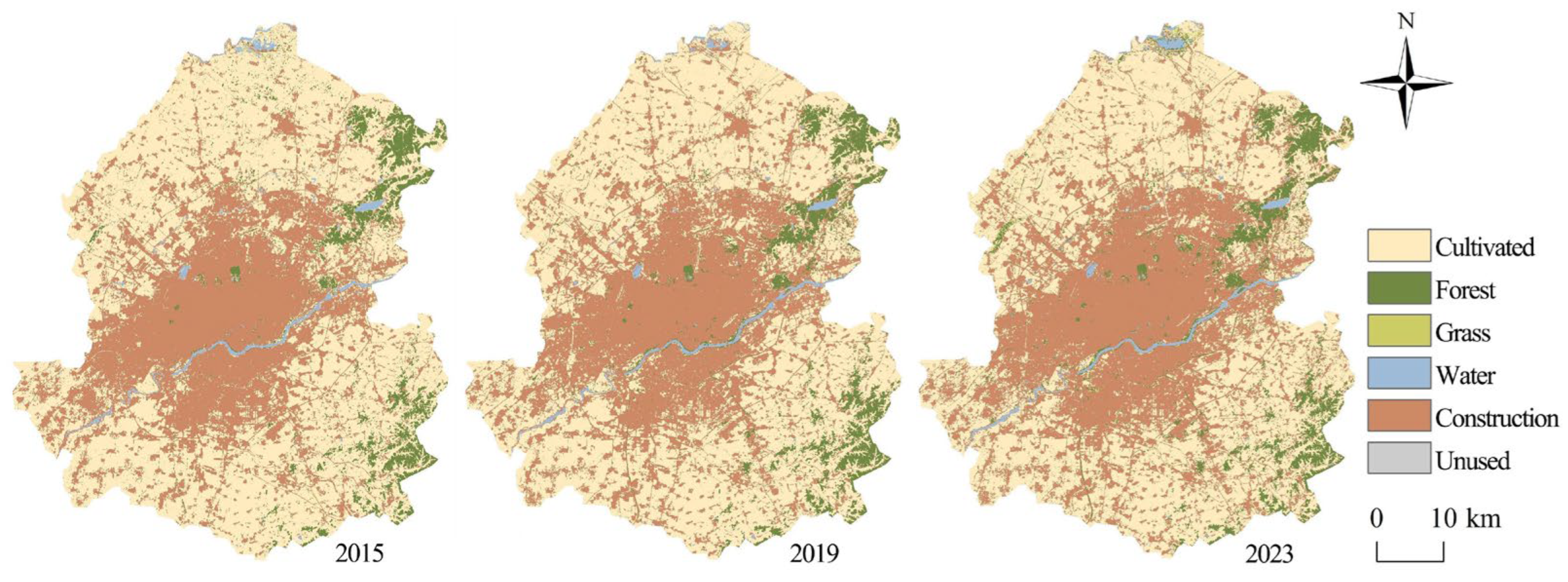
This study classifies land use into six distinct categories: cultivated land, forest, grassland, waterbody, construction land, and unused land (Figure 2). The classification process involved several key steps. First, remote sensing images with cloud cover less than 5% were selected, with the actual cloud cover in the study area being 0%. These images were then preprocessed through radiometric calibration and atmospheric correction. Supervised classification was performed on the preprocessed data, primarily using visual interpretation, in which land types were identified by establishing regions of interest and employing color composites from various band combinations. Subsequently, two classification algorithms—Support Vector Machines (SVM) and RF—were evaluated for performance. Using high-resolution Google Earth imagery from 2015 to 2024 (http://www.google.ca/earth/, accessed on 15 January 2025) as reference data, a kappa coefficient-based accuracy assessment revealed that the SVM method achieved an accuracy of approximately 85%, while the RF method exceeded 90%. Based on this comparison, the RF algorithm was selected for final land classification, and Figure 2 was generated accordingly. All classification and image processing tasks were carried out using ENVI 5.3. The data were obtained from official publications and public databases (see

Table 1. Information table of data sources.

Data Name	Data Source	Data Type	Resolution
Administrative Boundaries	National Platform for Common Geospatial Information Services (www.tianditu.gov.cn, accessed on 10 January 2025)	Shpfile	/
Remote Sensing Data	Landsat8-9 OLI_TIRS Satellite Imagery	Raster	30 m
DEM	Geospatial Data Cloud (https://www.gscloud.cn, accessed on 11 January 2025)	Raster	30 m
Precipitation, Annual Average Evapotranspiration, Soil Data, and PM2.5	National Tibetan Plateau Scientific Data Center (https://data.tpdc.ac.cn, accessed on 28 January 2025)	Raster	1000 m
Population Density	LandScan (https://landscan.ornl.gov, accessed on 1 February 2025)	Raster	1000 m
GDP	Geographical Remote Sensing Ecology Network Platform (gisrs.cn, accessed on 1 February 2025)	Raster	1000 m
Water Consumption Data	Liaoning Province Water Resources Bulletin	Text	/
Night Light Index	Harvard Dataverse [28]	Raster	1000 m

), and underwent preprocessing steps including data cleaning. To ensure consistency, all raster data were projected to the WGS_1984_UTM_Zone_51N coordinate system and resampled to a spatial resolution of 30 m. The evaluation of ES supply and demand was conducted using the ArcGIS 10.8 platform.

2.3. Methods

The research framework of this study consists of four key components: (1) utilizing multi-source data, the InVEST model, and existing technologies to evaluate the spatial variation trends of landscape pattern indices and the ES supply–demand relationship from 2015 to 2023; (2) applying correlation analysis to identify the key landscape pattern indices that influence the positive development of ES supply and demand; (3) analyzing the driving mechanisms of these key indices on ESs using the XGBoost-SHAP model; and (4) conducting visual interpretation combined with the LOWESS method to clarify both the driving mechanisms and threshold effects of landscape pattern indices in areas exhibiting positive ES development. The logical structure of the research framework is illustrated in Figure 3.

2.3.1. The Landscape Index

Landscape indices are quantitative metrics that effectively summarize information about landscape patterns, capturing both the structural composition and spatial configuration of the landscape [29]. These indices enable comprehensive analysis and evaluation of landscape patterns across various spatial scales, providing a scientific foundation for landscape ecology research and management planning. Due to the wide variety of landscape indices, they are typically categorized into three levels of analysis: patch level, patch type level (class level), and landscape level. Based on the objectives of this study, the geographical environment, land use characteristics of Shenyang, and principles such as functional relevance, interpretability, non-redundancy, and stability, seven patch-type-level indices were selected. These include indices reflecting landscape composition—percentage of landscape (PLAND), patch density (PD), and largest patch index (LPI); shape and edge complexity—landscape shape index (LSI) and edge density (ED); and spatial distribution—aggregation index (AI) and interspersion and juxtaposition index (IJI). These indices, calculated using the Fragstats 4.2 software, provide key insights into the spatial patterns and structural dynamics of landscapes. Detailed definitions of these indices are presented in

Table 2. Meanings and calculation methods of landscape indices.

Landscape Index	Abbreviation	Meaning	Calculation Formula
Aggregation Index	AI	AI examines the connectivity between patches of each landscape type. A smaller value indicates a more discrete landscape.	$AI=\left[{\displaystyle \frac{g_{ii}}{max\to g_{ii}}}\right]$ $g_{ii}$ represents the number of similar adjacent patches of the corresponding landscape type, 0 < AI ≤ 100.
Edge density	ED	The length of patch boundaries per unit area directly characterizes the overall complexity of the landscape.	$ED={\displaystyle \frac{E}{A}}$ E is the total length of patch boundaries in the landscape; A is the total landscape area; ED ≥ 0, unbounded, m/ha.
Interspersion and juxtaposition index	IJI	A measure of landscape isolation and patch mixing. A larger index indicates more obvious patterns of alternating different patches and higher patch dispersion.	$IJI={\displaystyle \frac{-{{\displaystyle \sum }}_{i=1}^m{{\displaystyle \sum }}_{k=i+1}^m\left[\left(\frac{e_{ik}}{E}\right)\right]·\ln \frac{e_{ik}}{E}}{\ln \left[0.5\left(m-1\right)\right]}}\times 100$ $e_{ik}$ is the total edge length between patches i and k, E is the total edge length in the entire landscape (excluding the background), and m is the number of patch types, 0 < IJI ≤ 100,%.
Largest patch index	LPI	Identifies the dominant patch type in the landscape. The index value helps determine the dominant patch type and indirectly reflects the direction and intensity of human activity interference.	$LPI={\displaystyle \frac{Max\left(a_1\dots a_n\right)}{A}}\times 100$ $Max\left(a_1\dots a_n\right)$ is the area of the largest patch; A is the total landscape area; 0 ≤ LPI ≤ 100,%.
Landscape shape index	LSI	The value increases as the landscape shape becomes more irregular or deviates further from a square.	$LSI={\displaystyle \frac{0.25E}{\sqrt{A}}}$ E is the total length of all patch boundaries in the landscape; A is the total landscape area. LSI ≥ 1, unbounded.
Patch density	PD	The degree of patch aggregation within a specific range. Within a particular study area, a higher density indicates a larger total number of patches.	$PD={\displaystyle \frac{N}{A}}$ N is the total number of patches in the landscape; A is the total landscape area; PD > 0, pcs/100 ha, unbounded.
Percentage of landscape	PLAND	When the patch area percentage approaches zero, it indicates a decrease in the occurrence of that patch type. A value of 100 means the entire landscape consists of only one patch type.	$PLAND={\displaystyle \frac{{{\displaystyle \sum }}_{j=1}^n{a}_{ij}}{A}}\times 100$ aij is the area of the j-th patch in the i-th landscape type; A is the total landscape area,%.

.

To clarify the spatial heterogeneity of landscape patterns and the relationship between landscape indices and spatial variables, this study employs the moving window method for further analysis. Raster data for landscape indices are calculated using this approach to capture local spatial variability. The selection of an appropriate window size is guided by semivariogram analysis, ensuring that the dominant spatial scale of key ecological processes is accurately represented. Specifically, the 2023 land use classification raster data serve as the foundation. Following the methodologies of Li, Zhou, and Wang [30,31,32], the LSI, PD, and Shannon’s Diversity Index are calculated at the overall landscape level. The moving window radii are set to 300, 600, 900, 1200, 1500, and 1800 m, and the indices are computed for each radius in sequence. The spatial variation characteristics of each index across different scales are then examined using semivariogram models. Based on the comparative analysis of these models, a window radius of 900 m is identified as the optimal analysis extent for capturing landscape patterns in the study area.

2.3.2. Assessment of Ecosystem Service Supply and Demand

After reviewing Shenyang’s ecological protection plans and environmental quality reports from the past decade, four critical ecological and environmental challenges have been identified. Firstly, the city faces a severe water shortage; according to the 2024 World Water Development Report, 25% of the global population experiences “extreme” water scarcity, with water utilization rates exceeding 80% in those areas. Shenyang’s per capita water availability is only one-sixth of the national average, classifying it as one of the most water-stressed regions in northern China. Secondly, over the past decade, Shenyang has encountered numerous extreme weather events, including prolonged cold spells, dust storms, intense rainfall, and severe snowstorms. Notably, in 2021, the city recorded its most intense snowfall since 1905, and in 2024, it experienced a rainstorm with a return period of 73 years. These events threaten urban safety, disrupt agricultural production, and affect residents’ daily lives. Thirdly, despite continued efforts to improve environmental quality, Shenyang still grapples with high levels of pollutants and carbon emissions. Its dependency on coal-based energy and a sluggish transition in industrial structure contribute to limited and fragile environmental gains, leaving the ecological landscape in a precarious state. Finally, the region’s natural environment is both fragile and highly sensitive, with significant degradation in several ecosystems. Ongoing urban expansion has reduced the size and connectivity of natural habitats, leading to habitat fragmentation, loss of biodiversity, and weakened ESs, all of which diminish the environment’s capacity to sustainably support human well-being.

After reviewing Shenyang’s ecological protection plans and environmental quality reports from the past decade, we identified four critical issues that underscore the region’s environmental vulnerability. In response to these pressing challenges, we selected five key ESs for in-depth study, WR, FR, AP, CS, and HQ. These services were chosen based on their relevance to Shenyang’s environmental context and their potential to address the city’s most urgent ecological concerns. The following section summarizes the methods used to calculate and analyze each of these ESs:

(1)

WR

Supply: The calculation is based on the water balance equation [33,34], which adheres to the principle of mass conservation. According to this principle, within a defined spatial and temporal scope, the difference between the water input and output of a system equals the change in the system’s water storage.

$$S_{WR}={\displaystyle \sum }_{i=1}^n{A}_i\times \left(P_i-E{T}_i-R_i\right)\times {10}^{-3}$$

(1)

$S_{WR}$ represents the annual water conservation amount (m³/a); $A_i$ is the area of land use type i (m²); P_i denotes annual rainfall (mm/a); $R_i$ is surface runoff (mm/a); ET_i stands for evapotranspiration (mm/a); i refers to the specific ecosystem type, and n indicates the total number of ecosystem types.

Demand: For demand estimation, the total water consumption for industrial, domestic, and agricultural sectors within the assessment year is evaluated. This demand is then spatially distributed across corresponding land use categories, including industrial land, residential areas, cultivated land, and ecological zones, enabling a rasterized representation of water conservation demand [1,35].

$$D_i=D_{agr,i}+D_{dom,i}+D_{ind,i}$$

(2)

$D_{agr,i}$, $D_{dom,i}$ and $D_{ind,i}$ represent the annual average agricultural, domestic and industrial water consumption per unit area for grid cell i.

(2)

FR

Supply: The stormwater regulation capacity is closely influenced by factors such as storm precipitation, surface runoff, and land use types. In this study, the supply of stormwater regulation services provided by green spaces is evaluated using the following equation [36].

$$S_{FR}={{\displaystyle \sum }}_{i=1}^n{A}_i\times \left(P-R_i\right)\times {10}^{-3}$$

(3)

S_FR represents the stormwater regulation volume(m³/a); A_i is the area of land use type i(m²) P is the annual rainfall (mm/a); R_i is the surface runoff (mm/a); i denotes the land use type, and n is the total number of land use types.

Demand: This study adopts the standards outlined in the Shenyang Sponge City Planning and Design Guidelines (2023 Edition), which require that the annual total runoff control rate in the central urban area of Shenyang must not be lower than 80%. This benchmark serves as the basis for defining stormwater regulation demand. Following the approach of Kang Dan et al. [37], the total runoff control rate index is further disaggregated according to various land use types (

Table 3. Classification and assignment of decomposed targets for total annual runoff control rate.

Land Use Type		Catchment Type	Target Value of Annual Runoff Control Rate (%)	Rainfall-Runoff Coefficient
Cultivated		Green Space	85	0.15
Forest		Green Space	85	0.15
Grass		Green Space	85	0.15
Water		Water Surface	100	1.0
Construction		Hard Roof, Roads and Squares	75	0.9
Unused		Unpaved Dirt Roads	45	0.3
Total Control Rate	2015	-	82	-
	2019		81
	2023		81

), enabling a spatially explicit quantification of stormwater regulation service demand.

$$D_{FR}={{\displaystyle \sum }}_{i=1}^n{A}_i\times P\times {\rho }_i\times RC{R}_i\times {10}^{-3}$$

(4)

$D_{FR}$ represents the stormwater regulation demand (m³/a); Ai is the area of land use type i (m²); P denotes the annual rainfall (mm/a); ${\rho }_i$ is the rainfall-runoff coefficient corresponding to land use type i; and $RC{R}_i$ is the target value of the annual runoff control rate for land use type i.

(3)

AP

Supply: The primary air pollutant in Shenyang is fine particulate matter (PM2.5) [38], and this study evaluates the removal efficiency of PM2.5 across various land use types as a key indicator of the capacity for AP services.

$$S_{AP}=A_i\times P_i$$

(5)

$S_{AP}$ represents the supply of AP services (kg); $A_i$ denotes the area of land use type i (ha); and $P_i$ refers to the amount of particulate matter intercepted and absorbed by land use type i (kg/ha). The $P_i$ values used for different land use types are as follows: cultivated land—0.09, forest land—0.1, grassland—0.09, water bodies—0.01, construction land—0, and bare land—0.02 kg/ha [39,40].

The objective of this study is to determine the AP demand in the central urban area by calculating the difference between the actual PM2.5 concentration per grid and the allowable PM2.5 concentration specified by government targets [41].

$$D_{AP}=({\rho }_i-P{M}_{2.5,AQS})\times A_i\times H$$

(6)

D_AP represents the demand for AP services (kg), where ${\rho }_i$ is the pollutant concentration in grid i (kg/m³). According to GB3095-2012, the allowable annual average concentration of PM2.5 is 35 µg/m³. A_i denotes the area of land use type i (m²), and H is the distribution height of PM2.5, which is approximately 1153 m [42].

(4)

CS

Supply: The total carbon storage was quantified using the “Carbon Storage and Sequestration” module of the InVEST model, which incorporates data from four carbon pools: aboveground biomass, belowground biomass, soil carbon, and dead organic matter. By integrating these inputs, the model estimates the total carbon storage across the study area. The carbon storage per unit area for each land use type was derived from parameters reported in previous studies [43,44,45]. Detailed parameter values are provided in

Table 4. Carbon densities and carbon emission coefficients of various land use types in the study area (t/ha).

Land Use Type	Carbon Densities				Carbon Emission (Absorption) Coefficients
	${\mathit{C}}_{\mathit{a}\mathit{b}\mathit{o}\mathit{v}\mathit{e}}$	${\mathit{C}}_{\mathit{b}\mathit{e}\mathit{l}\mathit{o}\mathit{w}}$	${\mathit{C}}_{\mathit{s}\mathit{o}\mathit{i}\mathit{l}}$	${\mathit{C}}_{\mathit{d}\mathit{e}\mathit{a}\mathit{d}}$
Cultivated	4.75	8.12	33.51	0	0.461
Forest	60.08	30.06	160.97	2.21	−0.581
Grass	31.71	23.66	55.13	29.03	−0.021
Water	3.325	0.6125	168.335	0.3875	−0.253
Construction	5.777	2.90	8.497	0.77	159.38
Unused	2.26	9.03	14.66	0	−0.005

.

$$S_{CS}=C_{above}+C_{below}+C_{soil}+C_{dead}$$

(7)

$S_{CS}$ represents the supply of CS services (t), calculated as the sum of four carbon pools: $C_{above}$ for aboveground biomass carbon storage (t), $C_{below}$ for belowground biomass carbon storage (t), $C_{soil}$ for soil carbon storage (t), and $C_{dead}$ for dead organic matter carbon storage (t).

The demand for CS services is estimated using the carbon emission coefficient method proposed by the IPCC, which enables the calculation of direct carbon emissions for each land use type [46,47].

$$D_{CS}=A_{if}\times d_f$$

(8)

$D_{CS}$ represents the demand for CS services (t); $A_{if}$ denotes the area of land use type f within grid i (ha); and $d_f$ is the carbon emission coefficient associated with land use type f (t/ha).

(5)

HQ

Supply: The current study employs the HQ module of the InVEST model to assess HQ by evaluating both habitat suitability and degradation. Cultivated land, construction land, and unused land are identified as primary habitat stressors, with the sensitivity of various habitat types to these threats derived from existing literature [48,49,50]. The corresponding calculation formula is presented as follows:

$$S_{HQ}=H_j\times \left(1-{\displaystyle \frac{D_{xj}^z}{D_{xj}^z+k^z}}\right)$$

(9)

$S_{HQ}$ represents the demand for biodiversity conservation services, where $H_j$ denotes the habitat suitability of land use type j, D is the level of stress, x refers to the grid, z is the normalization constant, and k is the half-saturation constant, which is typically set to a default value of 0.5.

Demand: The selection of socio-economic variables plays a crucial role in describing the overall demand for HQ [51]. In this study, the indicators used for analysis include the proportion of land used for construction, population density, and the nighttime light index. To accurately capture the degree of human interference with ecosystems, the intensity of resource consumption, and human preferences, a logarithmic processing method is applied in the statistical analysis [52,53,54].

$$D_{HQ}=P_{al}\times lg\left(P_{pop}\right)\times lg\left(P_{nl}\right)$$

(10)

$P_{al}$,$P_{pop}$ and $P_{nl}$ represent the proportion of construction land, population density and night light index, respectively.

(6)

Ecological supply–demand ratio (ESDR)

This study employs the ESDR to illustrate the matching relationship between the supply and demand of a specific ES [55], with the calculation formula presented as follows:

$$ESDR={\displaystyle \frac{S-D}{\left(S_{max}+D_{max}\right)/2}}$$

(11)

S and D represent the actual supply and demand of ESs within each grid cell, respectively, while S_max and D_max denote the maximum values of actual supply and demand across the entire study area. An ESDR value greater than 0 indicates a supply surplus, a value less than 0 reflects a supply deficit, and a value equal to 0 signifies a balance between supply and demand.

2.3.3. Spatial Variation Trend

The Theil–Sen Median Slope Estimation is a non-parametric statistical method widely used for analyzing trends in time-series data and offers significant advantages in assessing temporal changes in raster datasets [56]. This method is particularly robust against outliers, requires no assumptions regarding the underlying probability distribution of the data, and supports pixel-level calculations. In this study, the Theil–Sen method was applied to examine the spatial variation trends of the ESDR and various landscape metrics using data from the years 2015, 2019, and 2023.

$$\beta =\mathrm{Median}\left(\frac{x_j-x_i}{j-i}\right), \forall j>i$$

(12)

Median () The symbol β denotes the median of the pairwise slopes calculated from time-series data, where xi and xj represent individual data points within the series. A β value greater than 0 indicates an upward trend in the raster data over time; a β value less than 0 signifies a downward trend; and a β value equal to 0 suggests no change in the raster data throughout the time series.

The analysis results indicate that an increasing trend in the ESDR over time reflects an improving supply–demand relationship for ESs, moving toward a surplus or equilibrium, which signifies an enhancement in ecosystem functionality. Conversely, a declining ESDR suggests a deteriorating relationship, indicating a potential deficit in ES provision. A ratio of zero implies no change in the supply–demand dynamics. The primary objective of this study is to improve ESs by focusing on areas exhibiting an increasing ESDR, which are used as the dependent variable for further analysis. There are five potential scenarios associated with an increase in ESDR (

Table 5. The relationship between changes in supply and demand when ESDR increases.

Case	Supply	Demand	Coincident Conditions
1	+	+	S+ > D
2	+	Unchanged	None
3	+	−	None
4	Unchanged	−	None
5	−	−	S− < D−

The symbol “+” is used to indicate an increasing trend in the supply–demand ratio over time, while “−” is used to indicate a decreasing trend.

): (1) both supply and demand increase, with supply increasing more than demand; (2) supply increases while demand remains unchanged; (3) supply increases while demand decreases; (4) supply decreases while demand also decreases; and (5) both supply and demand decrease, but the decrease in supply is smaller than that in demand. It is important to note that this study addresses only scenarios 1, 3, and 5.

2.3.4. Driving Forces and Threshold Analysis Methods

(1)

Screening of potential landscape characteristic factors

A variety of factors influence the relationship between landscape metrics and the ESDR across different landscape types. Prior to analyzing the non-linear relationships between ESDR and landscape characteristics, Pearson correlation coefficients were calculated to assess the strength and significance of the correlation between ESDR and each landscape metric [57]. The Pearson correlation coefficient ranges from –1 to 1, indicating both the direction and strength of the relationship between two variables: a negative value signifies that one variable decreases as the other increases, a positive value indicates that both variables increase simultaneously, and a value of 0 denotes no correlation. All statistical calculations were performed using SPSS Statistics 27 software.

$${\rho }_{x,y}={\displaystyle \frac{COV\left(x,y\right)}{{\sigma }_x{\sigma }_y}}$$

(13)

$$r={\displaystyle \frac{{{\displaystyle \sum }}_{i=1}^n\left(x_i-\overline{x}\right)\left(y_i-\overline{y}\right)}{\sqrt{{{\displaystyle \sum }}_{i=1}^n{\left(x_i-\overline{x}\right)}^2{{\displaystyle \sum }}_{i=1}^n{\left(y_i-\overline{y}\right)}^2}}}$$

(14)

where ${\rho }_{x,y}$ represents the population correlation coefficient, where $COV\left(x,y\right)$ denotes the covariance between variables x and y, ${\sigma }_x$ is the standard deviation of x, and ${\sigma }_y$ is the standard deviation of y. The Pearson correlation coefficient r is estimated by calculating the covariance and standard deviations from the sample data. In this context, $x_i$ and $y_i$ refer to the i-th data points of variables x and y, respectively; $\overline{x}$ and $\overline{y}$ represent the mean values of x and y; and nnn is the sample size.

(2)

Driving Force Analysis Based on XGBoost-SHAP

The combination of XGBoost and SHAP has been widely applied to analyze the factors influencing ESs [58]. XGBoost, short for eXtreme Gradient Boosting, is an ensemble learning algorithm based on the Gradient Boosting Decision Tree framework. This method involves the iterative training of multiple decision trees, where each subsequent tree learns from the residuals, the differences between the predicted and actual values, of the previous model. The final prediction is generated through a weighted summation of all trees, resembling a collaborative process in which successive trees correct the errors of their predecessors [59,60].

SHAP values (Shapley Additive Explanations) offer a game theory-based approach for interpreting the outputs of machine learning models. They link optimal credit allocation with local interpretability by leveraging the classical Shapley value and its extensions [61]. SHAP values calculate the average marginal contribution of each feature to a model’s prediction, enabling a clear assessment of each feature’s importance in the decision-making process.

(3)

Threshold Analysis

Locally Weighted Scatterplot Smoothing (LOWESS) is a non-parametric local regression technique designed to improve the interpretability of scatterplots by applying weighted linear regression to the local neighborhood of data points [62]. This method effectively captures localized trends within the data. It offers two key advantages: it does not require any assumptions about the underlying data distribution, and it can flexibly model non-linear relationships, making it highly robust against noise. To better illustrate the complex, non-linear relationship between landscape characteristics and the ESDR, a LOWESS fitting curve can be incorporated into the SHAP dependency plot. This curve, generated through locally weighted regression, smooths fluctuations between data points and intuitively reveals trend directions and threshold effects within the data.

The intersection of the LOWESS curve with the SHAP value zero line (y = 0) holds particular analytical significance. The direction of the curve, whether it takes on positive or negative values, on either side of this intersection indicates how the feature influences the model’s predictions across different value intervals. For example, if the LOWESS curve for a specific feature intersects the zero line at a point denoted as x₀, this point can be considered a “critical threshold,” beyond which the feature begins to significantly influence the model’s output. When the feature value is less than x₀, it suggests that the feature has minimal or even inverse influence on the prediction. Additionally, the amplitude of the curve’s fluctuations, reflected in the range of absolute SHAP values, indicates the strength of the feature’s contribution to the model’s output. Larger fluctuations correspond to greater predictive importance under varying conditions. As such, this fluctuation range serves as a key indicator of the feature’s impact and can be considered a crucial driving factor within the model.

3. Results

3.1. Spatiotemporal Differentiation Characteristics of Landscape Patterns

3.1.1. Temporal Differentiation Characteristics

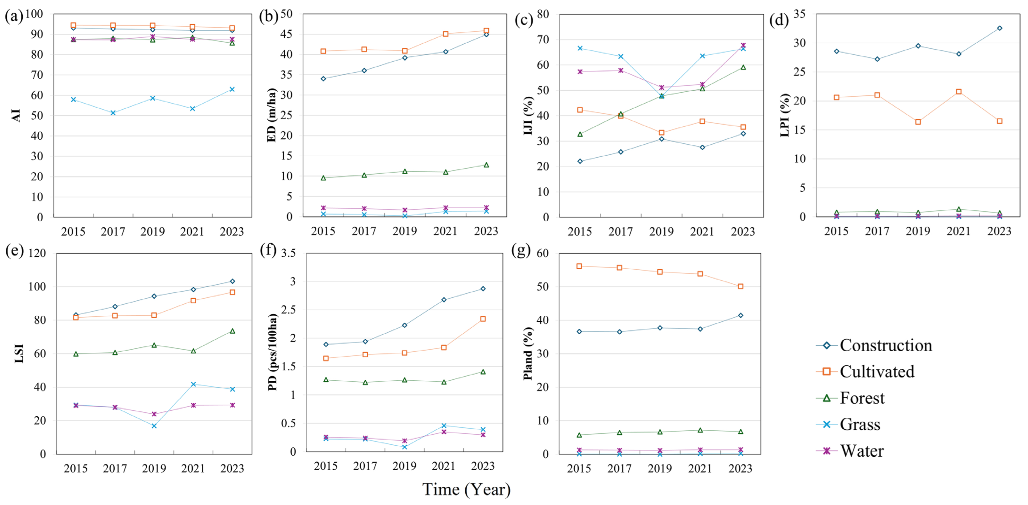
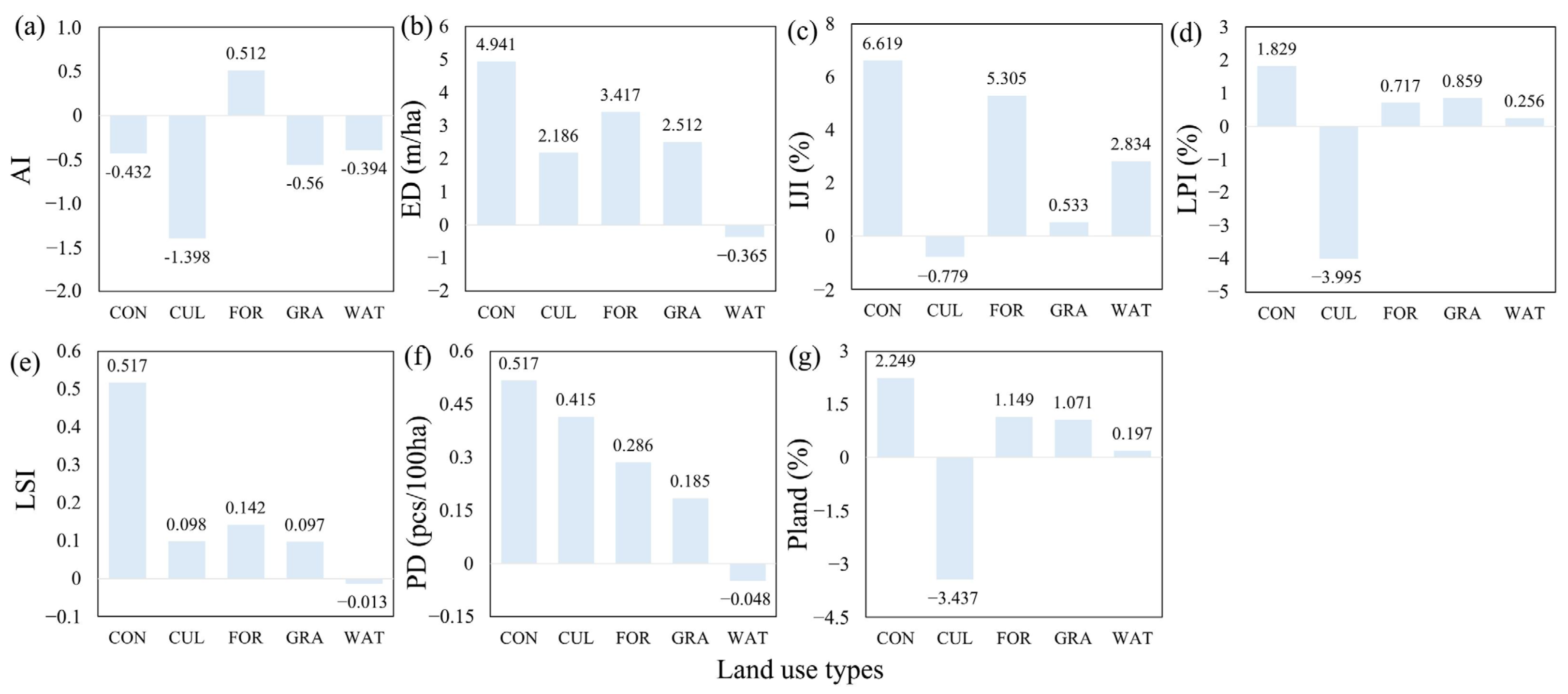
From 2015 to 2023, the annual average landscape indices for various land types exhibited distinct trends (Figure 4 and Figure 5). The indices for construction land, cultivated land, grassland, and water areas all declined to varying degrees. Grassland, in particular, showed lower average index values with significant fluctuations, recording an annual average dispersion rate of 29%. In contrast, forest land exhibited a decreasing dispersion trend initially, which later reversed, indicating an overall increase. The ED of construction land, cultivated land, forest land, and grassland showed a general upward trend, while the ED of water areas remained relatively stable. Among these, construction land had the highest annual average dispersion rate at approximately 37%, followed by grassland at around 23%. The LSI for construction land, cultivated land, and forest land also demonstrated an overall upward trend, suggesting increasing shape complexity. However, grassland LSI initially declined and then rose again, indicating a higher susceptibility to disturbances. Water areas showed negligible change in LSI. A comprehensive analysis of ED and LSI reveals that, apart from water areas, the spatial patterns of other land types have become increasingly complex and fragmented. The IJI for grassland and water areas remained high, indicating poor spatial aggregation in the study area. The IJI for forest land increased by 5.305, suggesting greater spatial dispersion and reduced homogeneity. Meanwhile, the IJI for cultivated land decreased initially, followed by fluctuations, resulting in an overall decline of 0.779. For construction land, although the IJI rose initially and then fluctuated, it ultimately showed a net increase of 6.619, indicating a high level of patch aggregation despite having the lowest overall IJI. Lastly, the LPI for construction land exhibited a consistent upward trend, reinforcing its dominant role among the landscape types in the region.

3.1.2. Spatial Differentiation Characteristics

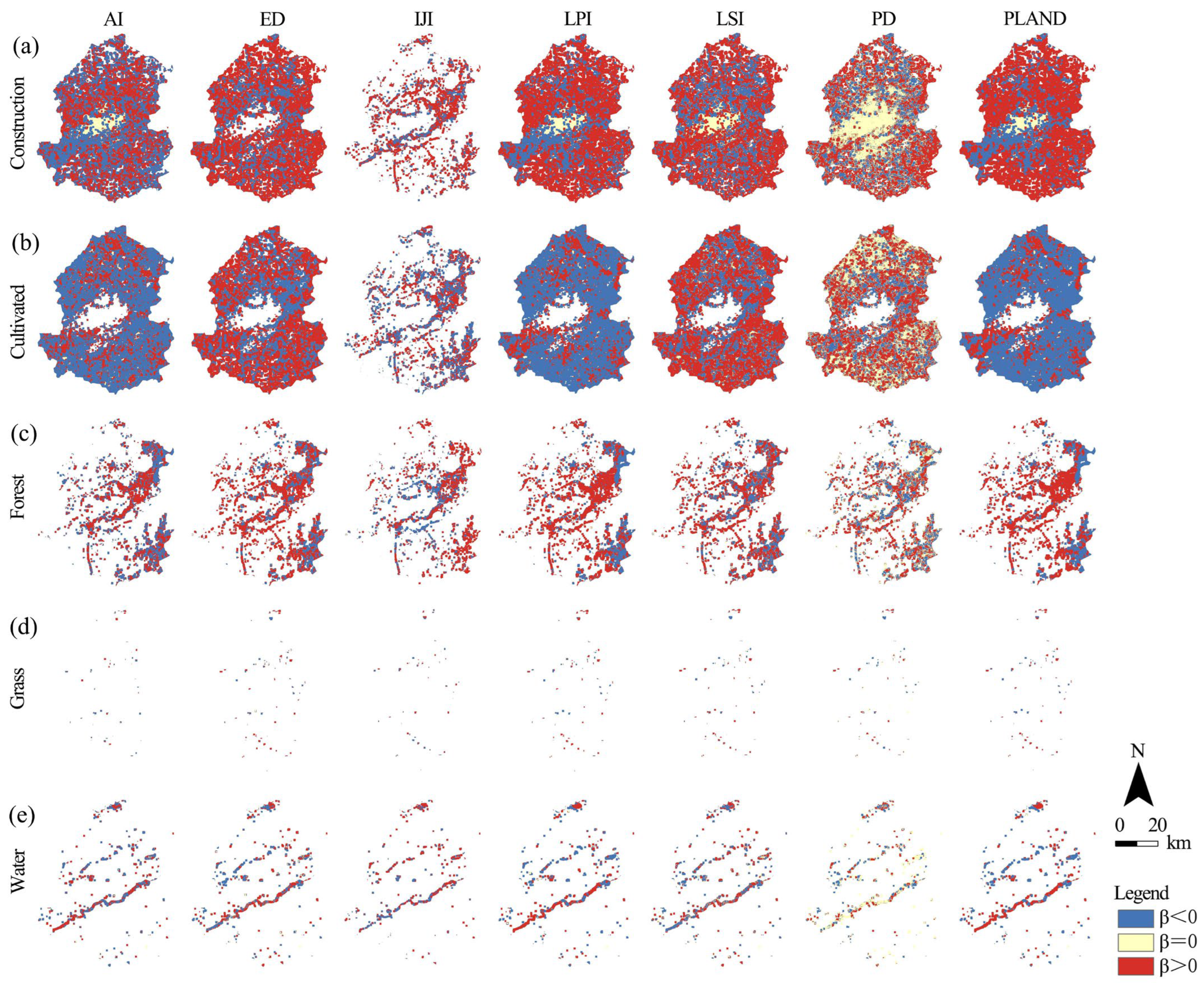
A spatial variation analysis of landscape indices across different land types reveals that each type exhibits distinct trends in its landscape characteristics (Figure 6). The specific findings are as follows:

From 2015 to 2023, spatial variation analysis of landscape indices across various land types revealed distinct and significant trends (Figure 6). Firstly, 72% of the area exhibited a decreasing trend in the AI for cultivated land (AI_CUL), with this trend evenly distributed across the study area, indicating an overall increase in landscape fragmentation. In contrast, approximately 52% of the area showed an increasing trend in the AI for forest land (AI_FOR), particularly in mountainous and hilly regions, suggesting improved landscape connectivity. Secondly, areas showing increases in ED, LSI, and PD for construction land, cultivated land, forest land, and grassland were mostly located outside the existing urban zones. This suggests that the spatial extent of these land types is expanding in peripheral areas, resulting in more complex edge structures and patch forms. Meanwhile, construction land in the older urban core showed minimal change. Additionally, water areas exhibited a decreasing trend, with significant reductions observed along the urban section of the Hun River. Thirdly, indices such as the IJI, LPI, and PLAND for construction land, forest land, grassland, and water areas all demonstrated upward trends, indicating increased intermixing of land patches. Spatially, construction land experienced notable dispersion outside the original urban footprint. The observed decline in LPI and PLAND within the Tiexi District suggests rising fragmentation and a consequent weakening of ecological functions. The IJI_FOR index showed greater dispersion in mountainous and hilly areas and near the Hun River, while elevated IJI_WAT values were found east of the river. Simultaneously, declining landscape indices for cultivated land point to heightened ecological vulnerability, especially in regions located in the northwest, east, and southwest portions of the study area.

In summary, the proportion of construction land has decreased, yet patch fragmentation persists alongside the presence of large core patches. These patches have become more complex in shape and are more evenly intermixed with other land uses. Cultivated land has experienced significant contraction, particularly in its largest patches, which have notably shrunk in size. The uniformity of adjacency with other land types has declined, while both fragmentation and shape complexity have intensified. Conversely, the area and number of forest patches have increased, with larger patches expanding and edge complexity rising. This has resulted in a heterogeneous spatial pattern characterized by large core forest patches surrounded by numerous smaller edge patches. Although the total grassland area has decreased, large core patches still remain, suggesting that grasslands are now more concentrated in central areas, while peripheral regions contain smaller, fragmented patches increasingly mixed with other land uses. Water bodies have shown a trend toward aggregation, forming substantial core areas with more regular shapes and reduced edge complexity. Additionally, the spatial uniformity of adjacent land uses surrounding water bodies has improved.

3.2. Spatiotemporal Differentiation Characteristics of ES Supply and Demand

3.2.1. Spatiotemporal Differentiation Characteristics of Supply

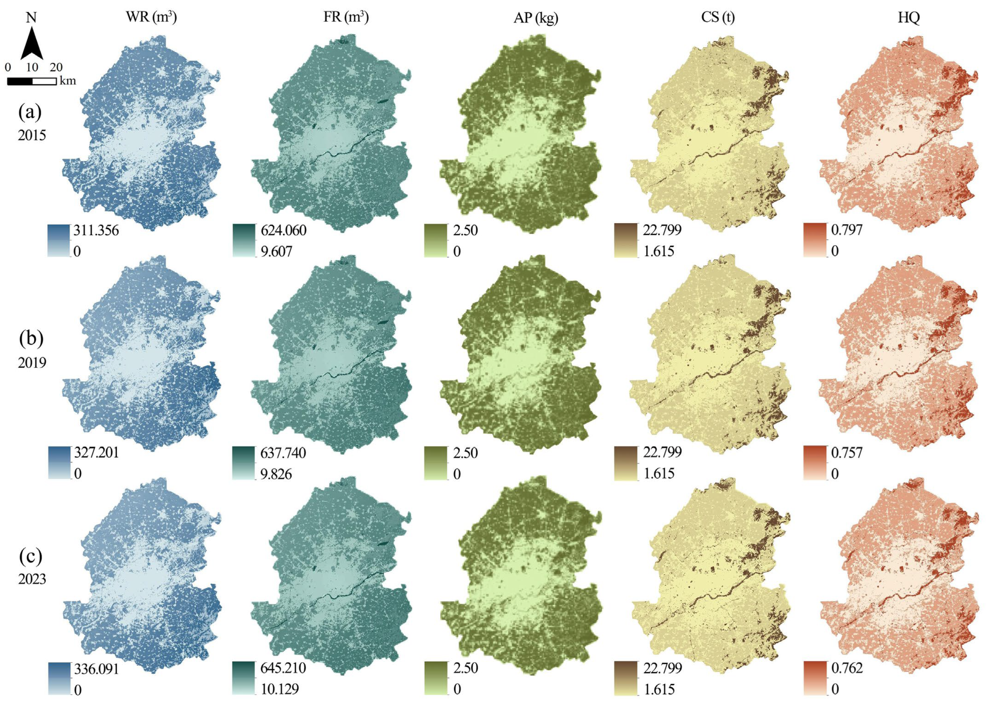
From 2015 to 2023, the supply of the five ESs exhibited significant spatial variation (Figure 7). In terms of value, the maximum supply capacities of Water Regulation (WR) and Food Regulation (FR) showed an upward trend over time. However, the changes in supply capacity for AP and CS were relatively insignificant, while the maximum supply capacity for HQ demonstrated a downward trend. Spatially, all five ESs consistently displayed low supply capacity in the central, older urban areas, with a radial distribution pattern extending outward toward surrounding regions. Higher supply capacities were observed in several districts, including Shenbei New District and Yuhong District in the south, as well as Hunnan New District and Sujiatun District in the north.

A detailed comparison of ESs revealed notable spatial and temporal shifts. In 2015, the highest Water Regulation (WR) supply capacities were observed in the southern part of Hunnan New District and the eastern part of Sujiatun District. By 2019 and 2023, these high-capacity areas had expanded to include the northern, eastern, and southern regions of Hunnan New District, as well as the eastern part of Sujiatun District. The spatial distribution of high-value Food Regulation (FR) supply areas generally followed the course of the Hun River. In 2015, FR supply capacity was relatively high in Tiexi District, Sujiatun District, and Hunnan New District; however, by 2019 and 2023, supply in Tiexi District had declined, while it had improved in the eastern part of Shenbei New District. The AP supply capacity remained strong in both the southern and northern areas of the central urban district, with little change over time, although some older urban sections experienced slight increases. The supply capacities of CS and HQ exhibited similar spatial trends, with high-supply areas concentrated along the Hun River and in surrounding hilly regions.

3.2.2. Spatiotemporal Differentiation Characteristics of Demand

Overall, from 2015 to 2023, the demand for the five ESs exhibited significant spatial heterogeneity (Figure 8). Spatially, the overall demand for Water Regulation (WR), Food Regulation (FR), CS, and HQ was relatively high in the older urban areas. Notably, the spatial distribution of demand for these services generally complemented the spatial pattern of their supply, highlighting a mismatch between areas of high demand and high supply.

A detailed comparison of the demand for each ES revealed notable temporal and spatial variations. Over time, the area with high demand for Water Regulation (WR) expanded. Initially, the maximum demand value decreased, then increased, ultimately becoming concentrated at the junction of Shenhe District, Heping District, Huanggu District, Dadong District, and Tiexi District. For Food Regulation (FR), demand initially rose before declining, with the highest demand observed along the Hun River, followed by areas at the urban expansion margins. In contrast, demand in the older urban areas and other regions remained relatively low. The spatial distribution of AP demand lacked a consistent pattern, but the overall trend showed a decline. The spatial changes in demand for CS and HQ followed similar patterns, with the highest demand concentrated in the central urban areas, gradually decreasing toward the outskirts. However, their spatial extents differed slightly. High-demand areas for CS were closely aligned with zones designated for construction land, while HQ demand, despite expanding in spatial coverage over time, experienced a consistent annual decline in maximum demand values.

3.2.3. Spatiotemporal Differentiation Characteristics of ESDR

The calculation results of the ESDR are illustrated in Figure 9. Recent studies highlight a persistent mismatch between supply and demand ratios within the central urban area. Overall, the study area shows a clear deficit in Water Regulation (WR), indicating a significant supply shortfall. In 2015 and 2019, WR supply surpluses were limited to the northern and southern peripheries, but by 2023, these surplus areas had further diminished, remaining only in the northeastern and southwestern parts, while the overall deficit deepened. From 2015 to 2023, the areas experiencing Food Regulation (FR) supply deficits were spatially similar to construction land, though the extent of high-value deficit zones gradually narrowed over time. FR supply surpluses remained concentrated in the southern and northern regions throughout the study period. In 2015, AP supply deficits were primarily found in five older urban districts and at the intersection of Sujiatun District, Hunnan New District, and the Hun River. These deficit areas decreased substantially by 2019, with continued improvement noted through 2023. CS also showed an overall supply deficit across the study area, with minor surpluses limited to mountainous and hilly regions; however, by 2023, supply surpluses had nearly disappeared. For HQ, the supply deficit area corresponded closely to construction land, but high-value deficit patches expanded each year toward the south and west. In contrast, high-value supply surplus areas remained concentrated in the mountainous and hilly regions.

Subsequent calculations were conducted to analyze the evolving trends of the ESDR from 2015 to 2023, as illustrated in Figure 10. The spatial variation in these trends revealed notable regional disparities. For ESDR related to Water Regulation (ESDR_WR), 15% of the regions exhibited an increasing trend, particularly in the southern part of Shenbei New District, the eastern part of Tiexi District, and the southern and southwestern areas of Hunnan New District. Additionally, areas near the junction of Heping District and Shenhe District also showed an upward trend. In contrast, a decreasing trend was observed in 14% of the regions, mainly within Huanggu District, Heping District, Shenhe District, and the southern part of Dadong District. The remaining 71% of regions showed no significant change in ESDR_WR. Regarding Food Regulation (ESDR_FR), 36% of regions demonstrated an increasing trend, especially in the eastern part of Tiexi District, southern Yuhong District, Heping District, southern Dadong District, Huanggu District, and selected areas of Shenbei and Hunnan New Districts. Meanwhile, 64% of regions showed a decreasing trend, primarily located in the northern, western, and southern portions of the study area. The ESDR_AP ratio increased in 50% of regions, notably within the five older urban districts. The other four administrative districts displayed a relatively even distribution between increasing and decreasing trends, with decreasing areas also constituting approximately 50%. For ESDR_CS, changes were concentrated in the central Tiexi District, southern Yuhong District, central Heping District, and western Hunnan District, accounting for 26% of the area. An upward trend was also observed in certain parts of Shenbei New District. However, decreasing trends were present in approximately 65% of the area, especially in Yuhong District, Shenbei New District, Hunnan New District, and Sujiatun District. Only 9% of the study area, located at the junction of the five older urban districts, showed no significant change. Lastly, for ESDR_HQ, 75% of regions experienced a decreasing trend, while 25% exhibited increases, primarily in the northern Shenbei New District, the junctions of Tiexi and Yuhong Districts, Heping and Shenhe Districts, along the Hun River, and in the southwestern part of Sujiatun District.

3.3. Results of Driving Mechanism Analysis

3.3.1. Screening of Landscape Characteristic Factors

An initial assessment of the correlation between landscape indices of various land types and the trend of ESDR increase was conducted using Pearson correlation coefficients (

Table 6. Pearson correlation coefficients between landscape indices of various land types and the increasing trend of ESDR.

Ecosystem Service	Land Use	AI	ED	IJI	LPI	LSI	PD	PLAND
WR	Construction	−0.026	−0.100 **	−0.089 **	−0.134 **	−0.069 **	−0.061	−0.161 **
	Cultivated	0.121 **	−0.005	0.014	0.148 **	−0.061	−0.073 **	0.173 **
	Forest	−0.004	−0.041	−0.046	−0.045	−0.029	0.002	−0.053
	Grass	−0.001	0.004	−0.01	−0.006	0.002	0.007	−0.004
	Water	0.068 **	0.027	0.060	0.013	−0.009	−0.007	0.02
FR	Construction	−0.209 **	0.112 **	−0.047 **	−0.678 **	0.253 **	0.156 **	−0.671 **
	Cultivated	0.164 **	0.156 **	−0.030	0.508 **	−0.047 **	−0.094 **	0.529 **
	Forest	0.015	0.066 **	−0.003	0.052 **	0.034	0.018	0.064 **
	Grass	0.007	0.012	−0.030	0.01	0.011	−0.002	0.01
	Water	−0.014	−0.067 **	−0.022	−0.02	−0.042 **	−0.012	−0.027
AP	Construction	−0.199 **	0.071 **	−0.01	−0.736 **	0.218 **	0.151 **	−0.745 **
	Cultivated	0.163 **	0.102 **	0.008	0.500 **	−0.074 **	−0.101 **	0.533 **
	Forest	0.033 **	0.096 **	0.002	0.092 **	0.054 **	0.021	0.112 **
	Grass	0.01	0.012	−0.023	0.001	0.013	0.004	0.008
	Water	0.004	−0.040 **	−0.023	0.017	−0.032 **	−0.009	0.013
CS	Construction	−0.302 **	−0.023	−0.055 **	−0.747 **	0.289 **	0.216 **	−0.762 **
	Cultivated	0.221 **	0.118 **	0.011	0.543 **	−0.116 **	−0.158 **	0.570 **
	Forest	0.026	0.03	0.021	0.041	−0.008	−0.013	0.041
	Grass	0.008	0.004	−0.031	−0.002	0	−0.007	0
	Water	0.016	0.01	−0.027	0.120 **	−0.029	−0.021	0.121 **
HQ	Construction	−0.083 **	0.079 **	0.175 **	−0.300 **	0.120 **	0.081 **	−0.291 **
	Cultivated	−0.080 **	0.027	0.044	0.002	0.059 **	0.067 **	−0.011
	Forest	0.104 **	0.275 **	0.096 **	0.276 **	0.184 **	0.041	0.308 **
	Grass	−0.006	0.063 **	−0.01	0.047 **	0.056 **	0.040	0.053 **
	Water	0.017	0.03	0.02	0.099 **	−0.006	0.009	0.104 **

** At the 0.01 level (two-tailed), the correlation is significant.

). Landscape indices with a p-value less than 0.01 were identified as potential driving factors influencing the ESDR growth trend. All seven landscape pattern indices associated with construction land showed significant correlations with ESDR changes for Food Regulation (FR) and HQ. Moreover, the LPI, LSI, PD, and PLAND for construction land, as well as the LSI for cultivated land, were significantly correlated with all five ESDR types. In contrast, landscape pattern indices for forest, grassland, and water exhibited fewer significant correlations with ESDR trends, likely due to the relatively limited distribution of these land types in the study area compared to construction and cultivated lands. Overall, a total of 10 landscape pattern indices were significantly associated with ESDR increases for Water Regulation (WR), 18 for FR, 19 for AP, 13 for CS, and 22 for HQ.

3.3.2. Correlation Between Landscape Characteristic Factors and ESs

In this study, the XGBoost-SHAP model was employed to investigate the relationship between changes in landscape indices and the supply–demand dynamics of ESs from 2015 to 2023. Given the data complexity and the model evaluation metrics, it was hypothesized that the model exhibited optimal explanatory power for Food Regulation (FR), AP, and CS, while demonstrating satisfactory performance for Water Regulation (WR) and HQ (

Table 7. Model performance evaluation indicators.

	Ecosystem Service	WR	FR	AP	CS	HQ
Model Evaluation Metrics
R2		0.478	0.598	0.728	0.703	0.355
MAE		0.007	0.011	0.026	0.042	0.048
MSE		0.0003	0.0003	0.002	0.004	0.006
RMSE		0.017	0.018	0.045	0.065	0.07

). The SHAP feature analysis of increasing trends in the five ESDR components, in conjunction with their corresponding landscape indices, revealed that the key driving factors varied across different ESDR types. To enable comparative analysis, the nine most influential landscape indices for each ESDR trend were selected for detailed interpretation (Figure 11).

The results reveal that area-based landscape indices, particularly PLAND and LPI, consistently rank among the top three most influential indicators for WR, FR, AP, and CS, and hold positions between second and fourth for HQ, underscoring their central role in driving changes in ESDR. However, the influence of these area indicators varies depending on land type; specifically, an increase in the area of construction land tends to exert a stronger inhibitory effect on the target values, whereas expansions in cultivated and forest land areas are associated with a more pronounced positive effect. Additionally, shape complexity, as reflected by the LSI, plays a substantial role in influencing target values. For example, LSI for construction land (LSI_CON) is negatively correlated with WR but positively associated with FR, AP, and CS, while LSI for cultivated land (LSI_CUL) exhibits the opposite pattern of influence. Moreover, aggregation metrics such as the AI and IJI, as well as edge-related indices like ED and PD, show varying degrees of impact across different ESDRs. For instance, ED_CON correlates negatively with WR and AP, whereas AI_CON demonstrates a positive association with FR and CS, and AI_CUL shows a negative relationship with HQ, highlighting the complex and differentiated influence of landscape structure on ES dynamics.

3.3.3. Threshold Effect of Landscape Characteristic Factors

The application of SHAP dependence plots combined with LOWESS curve fitting enables a more intuitive understanding of the non-linear relationships and threshold effects between key landscape features and ESDR increments. As illustrated in Figure 12, similar change patterns are observed for PLAND_CUL, LPI_CUL, and PLAND_CON. Specifically, when PLAND_CUL is below −1.51, LPI_CUL is below −1.24, and PLAND_CON falls below −9.20, the corresponding SHAP values are predominantly negative, indicating limited or even inhibitory effects on model predictions. Within the intermediate ranges, PLAND_CUL between −1.51 and 12.02, LPI_CUL between −1.24 and 2.73, and PLAND_CON between −9.20 and 0.44, SHAP values increase and reach their peak near zero, suggesting that the positive influence of these features is strongest within this range. However, beyond these upper thresholds (PLAND_CUL > 12.02, LPI_CUL > 2.73, PLAND_CON > 0.44), SHAP values begin to decline, implying a diminishing positive impact as feature values increase further. For LSI_CON, SHAP values are nearly neutral when the feature is below −0.41, indicating minimal influence. Between −0.10 and 0.13, SHAP values rise, peaking near the midpoint, but then decline beyond 0.13, reflecting a weakening effect. In the case of LPI_CON, values below −0.15 are associated with negative or neutral SHAP values, suggesting a suppressive role. Once LPI_CON exceeds −0.15, the LOWESS curve rises, and SHAP values become increasingly positive, indicating a growing positive effect. For ED_CON, SHAP values are slightly positive but low when the index is below −0.01, pointing to a weak positive contribution. When ED_CON exceeds −0.01, the LOWESS curve fluctuates modestly around zero, suggesting a neutral to mildly positive impact without a clear trend of increasing influence. Overall, these results underscore the complex and threshold-sensitive nature of landscape metrics in influencing ESDR dynamics.

In summary, the threshold ranges of variation in landscape characteristic factors that positively contribute to the increasing trend of ESDR in the WR region are as follows: PLAND_CUL ranges from −1.51 to 12.02, LPI_CUL from −1.24 to 2.73, PLAND_CON from −9.20 to 0.44, AI_CUL from 3.63 to 20, LSI_CON from −0.10 to 0.13, IJI_CON from 0.68 to 40, LPI_CON from −0.15 to 40, ED_CON from −20 to −0.01, and AI_WAT from 1.17 to 15.

SHAP dependence plots combined with LOWESS curve fitting were generated for the following landscape characteristic factors to analyze their influence on model predictions: (a) PLAND_CUL, (b) LPI_CUL, (c) PLAND_CON, (d) AI_CUL, (e) LSI_CON, (f) IJI_CON, (g) LPI_CON, (h) ED_CON, and (i) AI_WAT. Each plot illustrates the relationship between the modified values of a specific landscape factor and its corresponding SHAP value, thereby highlighting the nature and strength of its contribution to the model’s predictive outcomes across its observed value range.

As illustrated in Figure 13, the features PLAND_CON and LPI_CON exhibit similar patterns of variation: their SHAP values initially decrease sharply as the feature values increase, followed by a steady rise. Specifically, PLAND_CON contributes positively to the model’s predictions when its value is less than −1.45 or greater than 17.38, while LPI_CON has a positive influence when its value is less than −2.48. Conversely, within the range of −1.45 to 17.38 for PLAND_CON and values above −2.48 for LPI_CON, their contributions become negative, although the strength of their impact weakens. LPI_CUL displays a gradual upward trend that transitions into a sharp rise; it begins to positively influence model predictions when its value exceeds 1.52. Both LSI_CON and ED_CUL follow similar increasing trends, where rising values correspond to increasing SHAP values. Notably, the influence of LSI_CON and ED_CUL shifts from inhibitory to promotive at values of 0.16 and 1.63, respectively. In contrast, AI_CON exhibits a more complex pattern, with flat SHAP values at both ends and an inverted “V” shape in the middle. When AI_CON falls between −3.65 and −0.32, it positively contributes to model predictions. Meanwhile, LSI_CUL and PD_CON show opposite trends compared to LSI_CON and ED_CUL: as their values rise, their SHAP values decline. Their influence transitions from promotive to inhibitory at values of 0.01 for LSI_CUL and 0.37 for PD_CON. The variation pattern of AI_CUL is particularly intricate, comprising four distinct segments. It contributes positively to the model’s predictions when its value is less than −1.86 or within the range of 0.88 to 8.16.

In summary, the threshold ranges of variation in landscape characteristic factors that positively contribute to the increasing trend of ESDR in the FR region are as follows: PLAND_CON ranges from 20 to −1.45, LPI_CON from −30 to −2.48, LPI_CUL from 1.52 to 30, LSI_CON from 0.16 to 1.0, AI_CON from −3.65 to −0.32, LSI_CUL from −0.75 to 0.01, AI_CUL from 0.88 to 10, PD_CON from −5.0 to 0.37, and ED_CUL from 1.63 to 30.

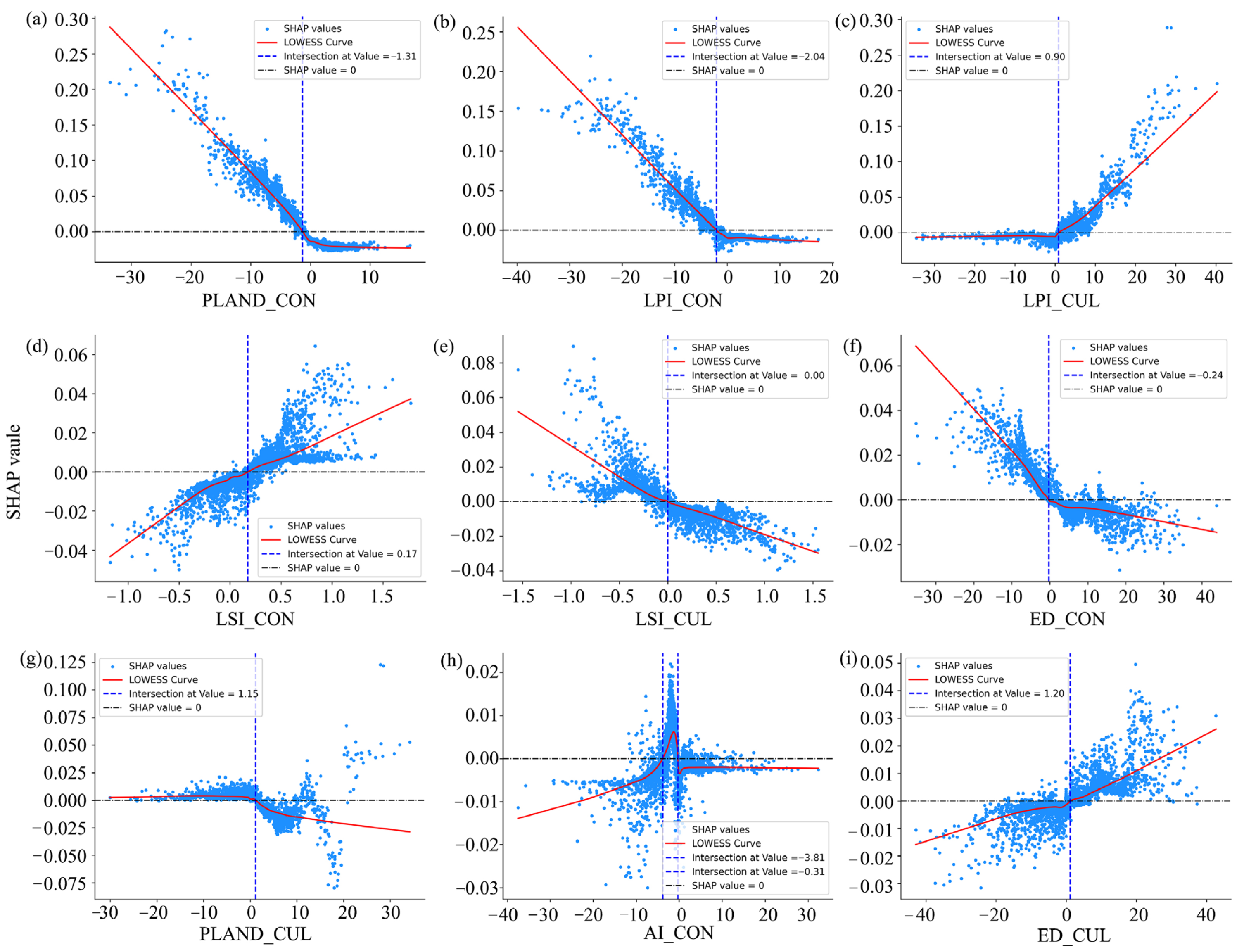
As illustrated in Figure 14, the relationship between PLAND_CON and its SHAP value reveals an initial sharp decline followed b y stabilization as PLAND_CON increases. Specifically, when PLAND_CON is less than −1.31, it contributes positively to the model’s prediction outcomes; however, as its value increases, its influence diminishes, eventually becoming negative. In contrast, an increase in ED_CON results in a pronounced drop in the SHAP value, which then transitions into a more gradual decline. When ED_CON falls below −0.24, it exerts a positive effect on the model’s predictions. The variation in PLAND_CUL is minimal within the range of −30 to 1.15, but once PLAND_CUL exceeds 1.15, its SHAP value steadily decreases, indicating a negative contribution to the model’s predictive performance and a stronger inhibiting effect. The trends for the remaining factors align with those observed in the FR region. The identified critical threshold values are as follows: −2.04 for LPI_CON, 0.90 for LPI_CUL, 0.17 for LSI_CON, 0 for LSI_CUL, and 1.20 for ED_CUL. Additionally, the critical range for AI_CON spans from −3.81 to −0.31.

In summary, the threshold ranges of variation in landscape characteristic factors that positively contribute to the increasing trend of ESDR in the AP region are as follows: PLAND_CON ranges from −20 to −1.31, LPI_CON from −30 to −2.04, LPI_CUL from 0.90 to 20, LSI_CON from 0.17 to 1.0, LSI_CUL from −0.75 to 0, ED_CON from −20 to −0.24, PLAND_CUL from −15 to 1.15, AI_CON from −3.81 to −0.31, and ED_CUL from 1.20 to 30.

As shown in Figure 15, the variation trends of most factors, except for AI_CUL, closely align with those observed for the landscape characteristic factors in the AP region. The identified critical values for PLAND_CON, LPI_CON, LPI_CUL, LSI_CUL, LSI_CON, PLAND_CUL, and ED_CUL are −2.72, −4.51, 2.39, −0.08, 0.28, 1.89, and 0.84, respectively. AI_CON positively contributes to the model’s prediction outcomes within the range of −3.52 to −0.50. In contrast, AI_CUL exhibits a more complex variation pattern, which can be divided into four distinct segments. Lower values of AI_CUL are associated with a stable positive effect on prediction results, while values approaching zero lead to increased fluctuation. As AI_CUL exceeds zero and continues to rise, its inhibitory effect on the model’s predictions becomes progressively stronger. Notably, AI_CUL positively contributes to prediction outcomes when its value lies within the ranges of −12.71 to −1.65 and 0.37 to 5.18.

In summary, the threshold ranges of variation in landscape characteristic factors that positively influence the increasing trend of ESDR in the CS region are identified as follows: In summary, the threshold ranges of variation in landscape characteristic factors that positively influence the increasing trend of ESDR in the CS region are identified as follows: PLAND_CON ranges from −20 to −2.72, LPI_CON from −25 to −4.51, LPI_CUL from 2.39 to 20, LSI_CUL from −0.75 to −0.08, LSI_CON from 0.28 to 1.0, AI_CON from −3.52 to −0.50, PLAND_CUL from −15 to 1.89, ED_CUL from 0.84 to 20, and AI_CUL either from −5 to −1.65 or from 0.37 to 5.18.

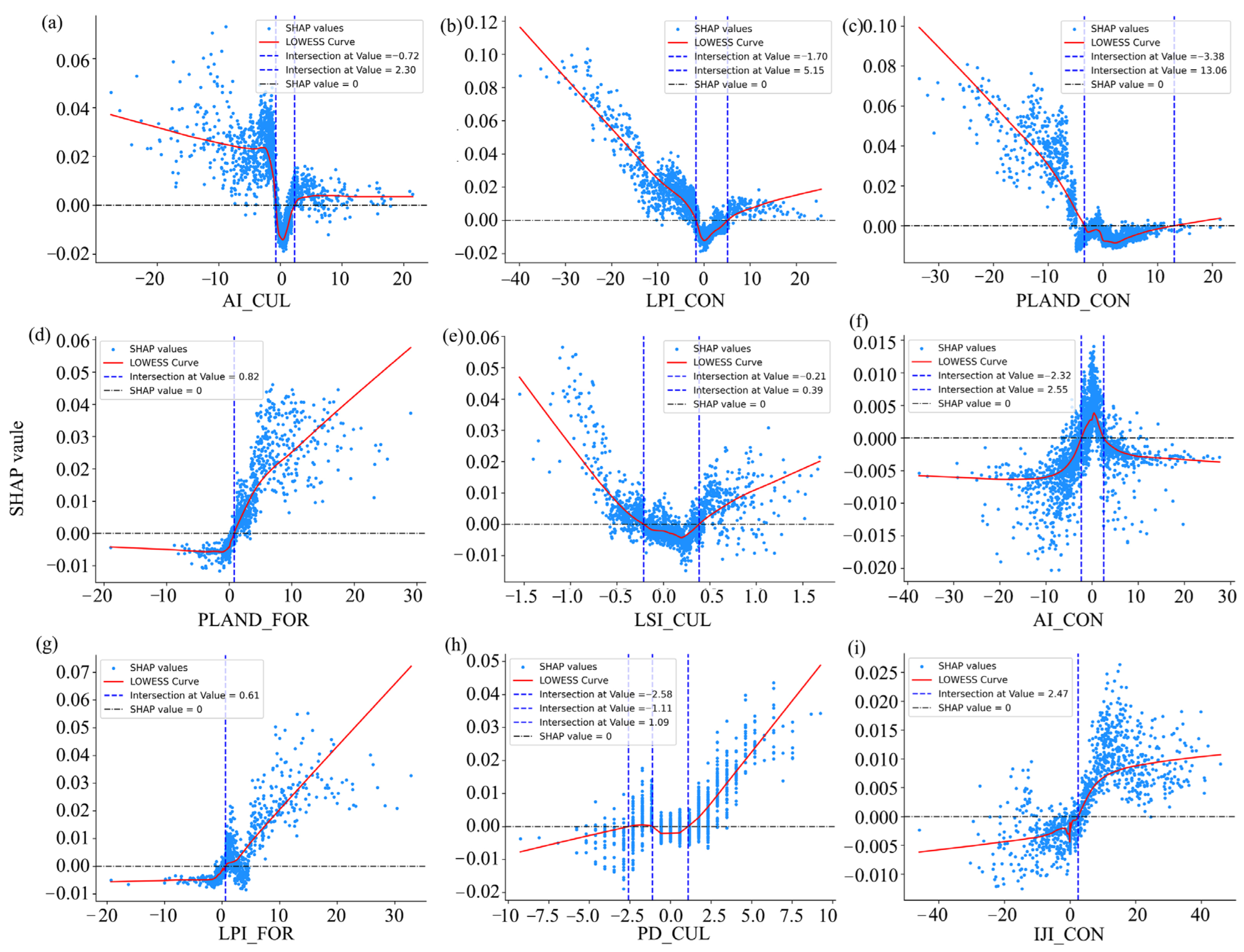
As illustrated in Figure 16, the variation trend of AI_CUL forms a “V” shape with flat ends. When the feature value is less than 0, it primarily enhances the prediction results, with the promotional effect becoming stronger as the value approaches 0. Conversely, when the feature value exceeds 0, the positive influence on prediction results diminishes, approaching a neutral effect. Specifically, AI_CUL values between −0.72 and 2.30 exert an inhibitory effect on the predictions, while values greater than 2.30 produce a leveling-off of the promotional impact. Similar variation patterns are observed in LPI_CON, PLAND_CON, and LSI_CON, where an initial sharp decrease in SHAP values is followed by a sharp increase as the feature values rise. For LPI_CON values below −1.70 or above 5.15, PLAND_CON values below −3.38 or above 13.06, and LSI_CON values below −0.21 or above 0.39, these features contribute positively to model predictions. In contrast, when LPI_CON is within −1.70 to 5.15, PLAND_CON from −3.38 to 13.06, and LSI_CON from −0.21 to 0.39, their contribution becomes negative. PLAND_FOR, LPI_FOR, IJI_CON, and PD_CUL exhibit similar trends: when their feature values are less than 0, SHAP values are predominantly negative; when values exceed 0, SHAP values are generally positive, and increasing feature values strengthen the promotional effect. However, distinct inflection points are noted for PLAND_FOR and IJI_CON at 5 and 10, respectively. Additionally, PD_CUL shows minor fluctuations in SHAP values, ranging from −2.58 to 0. The variation trend of AI_CON is characterized by flat ends and an inverted “V” shape in the middle, where values between −2.32 and 2.55 contribute positively to model prediction results.

In summary, the threshold ranges of variation in landscape characteristic factors that positively contribute to the increasing trend of ESDR in the HQ region are as follows: AI_CUL from −10 to −0.72, LPI_CON from −30 to −1.70, PLAND_CON from −20 to −5, PLAND_FOR from 0.82 to 20, LSI_CUL from −1.0 to −0.21, AI_CON from −2.32 to 2.55, LPI_FOR from 5 to 20, PD_CUL from 1.09 to 7.5, and IJI_CON from 2.47 to 20.

The present study primarily investigates the relationship between landscape characteristics and individual ESs. Overall, construction and cultivated land types exhibit a significant impact on ESs. Consequently, landscape characteristics that demonstrate a strong correlation with all five ESs were selected for further analysis, and their threshold effects were examined in detail (Figure 17).

The findings reveal that the impact of changes in landscape characteristics varies across different ESs. For cultivated land, the three threshold groups indicate that the sensitivity of LPI_CUL to FR, AP, and CS is relatively consistent, ranging from approximately 2.39% to 20%. In contrast, the threshold range influencing WR is narrower. Therefore, managing LPI_CUL with a synergistic strategy can effectively enhance these three ESs. Similarly, LSI_CUL exhibits comparable sensitivity to FR, AP, CS, and HQ, with values ranging from −0.75 to −0.21, suggesting that maintaining cultivated land in a more regular shape may optimize these four services. However, AI_CUL displays varied threshold ranges across different ESs, indicating that its impact should be analyzed in conjunction with spatial factors. For construction land, PLAND_CON shows consistent sensitivity to four ESs, where a reduction between 4.51% and 25% can improve service performance. In the case of LSI, which presents notable variability, an increase from 0.28 to 1 positively influences FR, AP, and CS, supporting a coordinated improvement strategy. Notably, HQ demonstrates high tolerance for AI_CON, implying that a reduction in AI_CON by 0.5 to 2.32 may enhance all four ESs.

4. Discussion

4.1. Interactive Relationship Between Landscape Pattern Indices and Supply–Demand of ESs

This study quantitatively analyzes the relationship between landscape pattern index variables and the increase in the ESDR, with the objective of enhancing ESs in the study area through the optimization of landscape patterns. Unlike previous research, which primarily emphasized the increase in ES supply, this study also incorporates the growth in ES demand. As a result, areas with favorable conditions for ESDR development are identified as priority targets for optimization, and the effects of changes in landscape characteristics on ESDR are systematically examined.

The results indicate a significant decline in the area of cultivated land within the study region. This reduction has led to the shrinkage of large patches and decreased uniformity in their adjacency to other land uses. At the same time, patch fragmentation and shape complexity have increased, which has impeded improvements in WR. While some studies suggest that an increase in cultivated land area could reduce WR supply capacity [63], this apparent contradiction may be explained by the role of management practices: well-maintained cultivated land, scientific crop planting, and optimized irrigation systems can minimize water loss, whereas poorly managed farmland, either abandoned or fragmented, tends to negatively affect WR. Moreover, a higher proportion of construction land correlates with increased shape complexity and edge irregularity. When construction land is interspersed with other land uses, its inhibitory effect on WR becomes even more pronounced. These findings are consistent with the observations made by Huang in Zhangjiakou [64].

In terms of FR, areas situated along rivers with flat terrain, as well as regions with high population density and GDP, tend to exhibit lower levels of FR [65]. Additionally, PM2.5 concentration is significantly negatively correlated with green quantity under similar environmental conditions [66]. This study finds that, despite a supply deficit in the older urban areas of Shenyang, both FR and AP are generally improving. This positive trend may be attributed to a three-year greening initiative conducted from 2016 to 2018, which focused on urban environmental enhancements, including the “Two Banks of One River” project, road upgrades, water system improvements, the creation of parks and landscape nodes, and the expansion of green coverage to address existing gaps [67]. In contrast, semi-built-up and suburban areas exhibit a supply surplus; however, many of these regions have begun to show signs of degradation. This suggests that during urban expansion, the increase in impervious surfaces and the decline in green spaces can contribute to the deterioration of both FR and AP [68].

In terms of CS, the urban CS system functions as an integrated entity composed of both natural ecological systems and artificially constructed components [69]. The overall CS capacity in the study area reflects a supply deficit, primarily due to the dominance of impervious surfaces associated with construction. The expansion of these areas not only encroaches upon natural landscapes but also increases landscape fragmentation, thereby diminishing CS potential. Cultivated land, as a managed open natural ecosystem, exhibits CS potential influenced by a range of factors, including climate conditions, soil types, management practices, and the timing of measurements [70]. In this study, we observed that an increase in the LPI of cultivated land, combined with a reduction in the shape index, significantly enhances the effectiveness of CS.

Habitat fragmentation, degradation, and loss are widely recognized as the primary drivers of biodiversity decline in terms of HQ [53,71]. In urban ecosystems, the expansion of construction areas and agricultural land exerts a detrimental effect on HQ by disrupting natural landscapes and reducing ecological connectivity. However, increasing the proportion of forested land has been shown to significantly improve HQ by restoring ecological balance, enhancing biodiversity, and providing stable, high-quality habitats for various species.

4.2. Driving Mechanism and Threshold Analysis

Urban landscape patterns are dynamic and represent the combined influence of socio-ecological factors on ESs [72]. Variables such as spatial type, area size, and vegetation configuration significantly affect the supply of different ESs. However, limited research has explored the threshold effects of landscape patterns on ESs in relation to varying demand levels, especially within the context of rapid urbanization. The ESDR is a valuable indicator for assessing the overall health and functionality of ESs. A thorough understanding of the threshold effects driving ESDR is crucial for examining human–land interactions and advancing sustainable urban development [73]. While previous studies have largely concentrated on the quantitative and spatial differences in supply–demand relationships from a static perspective, they often overlook temporal dynamics. For example, when the ESDR equals zero, the corresponding value of a driving factor at that point is considered optimal. One study found that CS reaches equilibrium when forest land comprises at least 80.38% of the area and developed land accounts for no more than 13.59% [74]. In this paper, we investigate the temporal evolution of the supply–demand relationship, identify regions with positive development potential, and leverage these insights for environmental management strategies. Additionally, we analyze the effects of various landscape pattern indices on these trends to uncover the underlying driving mechanisms and their associated thresholds.

This study employs the XGBoost-SHAP model to investigate the driving factors influencing landscape pattern indices related to five key ESs in the central urban area of Shenyang. The results demonstrate that the relationship between landscape pattern indices and ESs is not a simple linear correlation; instead, various indices exert differing degrees of influence, with clear threshold intervals beyond which their effects change significantly. For example, when the proportion of construction land decreases from 1.45% to 20%, its contribution to the positive development of FR increases. In contrast, if construction land expands from 1.45% to 10%, it negatively affects the positive development of FR. Similarly, an increase in the cultivated land shape index from 0.21 to 0.39 has an adverse impact on HQ, whereas a decrease from 0.21 to 1 or an increase from 0.39 to 1.5 positively contributes to HQ enhancement. These patterns suggest that within complex natural, social, economic, and ecological systems, scientific and precise land-use planning is essential for sustainable development. Although many studies have confirmed that expanding forest land can enhance ESs [9,75], the present findings reveal that when forest land exceeds a threshold proportion of 0.82, its positive influence on HQ becomes significantly stronger.

Landscape pattern indices are primarily based on land use data, which are generally accessible, reliable, and manageable for decision makers [75]. These indices offer adaptable thresholds that help guide efforts to enhance regional ESs. By evaluating the current state of ESs, managers can identify which landscape pattern indices require optimization and determine the extent of necessary adjustments. Defining such thresholds is crucial for achieving a balanced relationship between ecological preservation and urban development amid evolving natural and social conditions. Moreover, these indices serve as valuable tools for supporting environmental planning and play a vital role in promoting human well-being [76,77].

4.3. Development Suggestions

Urban development policies aimed at enhancing ESs are gaining increasing recognition, with growing integration into spatial planning, natural resource management, and land use decision making. This shift provides a strong foundation for promoting regional sustainable development and improving human well-being [78,79]. To effectively advance ESs, this study recommends regulating landscape patterns by identifying the sensitivity of various ESs to changes in specific landscape characteristics. This strategy should be tailored to the distinctive regional features of Shenyang’s central urban area to ensure targeted and context-specific improvements.

In the study area, the landscape pattern is transitioning from a predominantly “artificial land-dominated” configuration to a “natural–artificial mixed mosaic.” The expansion of forested areas and the incorporation of water bodies have emerged as key priorities for ecological restoration efforts. Simultaneously, reductions in construction and cultivated land are occurring alongside increasing landscape fragmentation, reflecting the combined influence of ecological protection policies and evolving land-use practices. However, it is essential to remain vigilant about the potential risks posed by the fragmentation of cultivated land and the inefficient utilization of construction land.

When regulating cultivated land, it is essential to ensure that the LPI ranges from 2.39% to 20%, while the shape index should be appropriately reduced within the range of 0.21 to 0.75. For fragmented patches of cultivated land, where increases in ED and PD are observed, consolidating smaller plots into larger, more cohesive units is recommended. Integrating forested areas into the design of ecological corridors can further support this strategy by establishing a landscape structure of “cultivated land core + ecological buffer zone.” This configuration not only enhances agricultural productivity and facilitates centralized management but also capitalizes on the strong root systems of tree vegetation to improve critical ecological functions such as soil stabilization and water conservation [80]. In optimizing construction land, the total area should ideally be reduced by 4.51% to 25%. For core built-up zones experiencing a rise in LPI, structural and configurational imbalances between impervious surfaces and green spaces should be addressed through the application of “Smart Growth” principles. Increasing the IJI of construction land and adopting a “greening in every available space” approach will significantly boost green space coverage. Enhancing both the quantity and quality of green space patches is essential to improving the supply of ESs [81,82]. Studies have shown that under identical PM2.5 concentrations, trees are more effective than grass at filtering airborne pollutants, making vertical greening particularly valuable in high-density built-up areas for improving AP [83]. Additionally, ecological reclamation should be implemented on fragmented construction patches with elevated PD, converting them into functional urban green spaces. For improved forest regulation, forest land area should be increased by approximately 5% to 20%, which can markedly enhance HQ. Strengthening connectivity between forested zones is also crucial. By increasing the IJI of forest and water bodies, biological corridors, such as forest trails and aquatic vegetation belts, can be developed to link fragmented patches, thereby mitigating the island effect associated with elevated PD and enhancing CS capacity [84,85]. Moreover, depending on road type and distribution, the implementation of strategies like patch integration and the creation of green buffers can help reduce landscape fragmentation caused by dense road networks [86].

4.4. Limitations and Prospects

This study offers targeted guidance for the spatial planning of Shenyang’s central urban area; however, it is not without limitations. First, the methods and data for ecosystem services (ESs) assessment have been revised based on previous studies and the actual situation in Shenyang. When applied in other regions, the data and methods should be adjusted in light of regional characteristics. Second, in terms of the research content, this study focused exclusively on analyzing the driving mechanisms and thresholds of a single landscape pattern index in relation to the spatiotemporal dynamics of the supply–demand relationship of one ES. In reality, multiple ESs often exhibit trade-offs and synergies, and their combined supply–demand relationships may respond differently to changes in landscape pattern indices. Furthermore, interactions among various landscape pattern indices may also influence these outcomes. Therefore, future research should explore the adaptability of the same ESs assessment method in different regions and the underlying reasons. Additionally, further investigation is needed into the spatiotemporal response mechanisms of a composite supply–demand index for multiple ESs in relation to landscape pattern indices, as well as the coupling relationships between ES improvements and multi-factor interactions. A more comprehensive and integrative approach will offer a stronger foundation for improving urban ecological environments and advancing sustainable urban development.

5. Conclusions

This study adopts a spatiotemporal dynamic approach to quantify changes in landscape patterns, as well as the supply, demand, and supply–demand ratio of five ESs in the central urban area of Shenyang. A key outcome is the identification of areas exhibiting an increasing supply–demand ratio, which are considered to hold strong potential for the development of ESs. By employing the XGBoost-SHAP model, this study visually explores the spatiotemporal responses of these areas to various landscape pattern indices and determines optimal thresholds using the LOWESS curve. This research offers both a scientific foundation and practical guidance for informed urban spatial planning and sustainable development. The primary conclusions drawn from this analysis are as follows:

(1)

The spatiotemporal distribution of landscape pattern indices at the patch-type level reveals significant differences across land types. Over time, the annual fluctuations of these indices vary by land category: construction land and forest areas have generally exhibited upward trends, while cultivated land has shown a consistent decline. Water bodies have remained relatively stable, whereas grassland has experienced the most pronounced fluctuations. In terms of spatial distribution, variations in the landscape indices are also evident due to the differing geographic locations of each land type, resulting in diverse patterns of change across the study area.

(2)

The supply, demand, and supply–demand relationships of different ESs exhibit significant spatial variation. Established urban areas typically experience a supply deficit but show strong potential for positive development. In contrast, emerging urban areas often demonstrate a supply surplus; however, they are trending toward unfavorable development. The proportions of favorable development zones for the supply–demand relationships of water regulation (WR), AP, FR, CS, and HQ are 14.5%, 35.8%, 50.2%, 25.6%, and 25.3%, respectively.

(3)

The influence of landscape pattern characteristics on ESs is distinctly non-linear, with each index exerting a unique effect and exhibiting clear threshold intervals. Among these factors, area-related indices, specifically PLAND and LPI, emerge as the primary drivers influencing the favorable development of ES supply–demand relationships. The shape index (LSI) ranks second in importance when determining target values. Other indices, such as AI, IJI, ED, and PD, show varying effects across different types of ESs, underscoring the complexity and context-specific nature of their impacts.

References

1. Wang, W.J.; Wang, G.Y.; Yang, M.L.; Mu, X.H.; Zhu, Z.W. Strategies of Critical Areas of Ecological Space in High-density Urban Areas from the Perspective of Ecosystem Supply and Demand, A Case Study of Guilin. Chin. Landsc. Archit. 2024, 40, 15–21. [Google Scholar]
2. Costanza, R.; d’Arge, R.; de Groot, R.; Belt, M. The value of the world’s ecosystem services and natural capital. Nature 1997, 387, 253–260. [Google Scholar] [CrossRef]
3. Su, C.; Fu, B.J. Discussion on Links Among Landscape Pattern, Ecological Process, and Ecosystem Services. Chin. J. Nat. 2012, 34, 277–283. [Google Scholar]
4. Castro, A.J.; Verburg, P.H.; Martín-López, B.; Garcia-Llorente, M.; Cabello, J.; Vaughn, C.C.; López, E. Ecosystem service trade-offs from supply to social demand: A landscape-scale spatial analysis. Landsc. Urban Plan. 2014, 132, 102–110. [Google Scholar] [CrossRef]
5. Baró, F.; Haase, D.; Gómez-Baggethun, E.; Frantzeskaki, N. Mismatches between ecosystem services supply and demand in urban areas: A quantitative assessment in five European cities. Ecol. Indic. 2015, 55, 146–158. [Google Scholar] [CrossRef]
6. Choumert, J. An empirical investigation of public choices for green spaces. Land Use Policy 2010, 27, 1123–1131. [Google Scholar] [CrossRef]
7. Cheng, C.N.; Hu, Y.; Zhao, M. Progress and prospect of the spatiotemporal change and ecosystem services evaluation of urban green space pattern. Prog. Geogr. 2020, 39, 1770–1782. [Google Scholar] [CrossRef]
8. Shao, M.; Li, F.Z.; Li, X. Evaluation of Supply and Demand of Green Space Ecosystem Service Function in Chengdu-Chongqing Urban Agglomeration Based on Multi-source Data. Landsc. Archit. 2021, 28, 60–66. [Google Scholar]
9. Liu, X.; Wang, K.; Qi, Z.X.; Li, T.; Li, S. Urban green space layout optimization based on ecosystem service supply and demand. J. Hunan Ecol. Sci. 2022, 9, 8–17. [Google Scholar]
10. Liu, Y.T.; Qin, M.L.; Ouyang, H.T. The optimization of territorial spatial resources allocation based on the balance of supply and demand of ecosystem services. J. Nat. Resour. 2024, 39, 1358–1383. [Google Scholar] [CrossRef]
11. Wang, X.K.; Su, Y.B.; Ren, Y.F.; Zhang, H.X.; Sun, X.; Ouyang, Z.Y. Urban ecosystem: Highly spatial heterogeneity. Acta Ecol. Sin. 2020, 40, 5103–5112. [Google Scholar]
12. Kirwan, M.L.; Megonigal, J.P. Tidal wetland stability in the face of human impacts and sea-level rise. Nature 2013, 504, 53–60. [Google Scholar] [CrossRef]
13. Yang, W.Q.; Yang, P.; Sun, X.; Han, B.L. Changes of landscape patter and its impacts on multiple ecosystem services in Beijing. Acta Ecol. Sin. 2022, 42, 6487–6498. [Google Scholar]
14. Su, S.L.; Xiao, R.; Jiang, Z.L.; Zhang, Y. Characterizing landscape pattern and ecosystem service value changes for urbanization impacts at an eco-regional scale. Appl. Geogr. 2012, 34, 295–305. [Google Scholar] [CrossRef]
15. Liang, Y.J.; Liu, L.J. Integration of ecosystem services and landscape pattern: A review. Acta Ecol. Sin. 2018, 38, 7159–7167. [Google Scholar] [CrossRef]
16. Ayinuer, Y.; Zhang, F.; Yu, H.Y.; Kung, H. Quantifying the spatial correlations between landscape pattern and ecosystem service value: A case study in Ebinur Lake Basin, Xinjiang, China. Ecol. Eng. 2018, 113, 94–104. [Google Scholar] [CrossRef]
17. Zhang, Z.Y.; Tong, Z.M.; Zhang, L.T.; Liu, Y.L. Nonlinear effects of landscape patter on ecosystem services and threshold regulation; a case study of eco-efficient synergistic zone in Fujian Province. Acta Ecol. Sin. 2024, 44, 9535–9551. [Google Scholar]
18. Wu, X.; Zhou, Z.X. Spatial relationship belween supply and demand of ecosystem services through urban green infrastructure: Case of Xi’ an Cily. Acta Ecol. Sin. 2019, 39, 9211–9221. [Google Scholar]
19. Xu, C.; Meng, N.; Lu, F. Research on Urban Green Infrastructure Management in Macao from the Perspective of Ecosystem Service Demand. Chin. Landsc. Archit. 2020, 36, 104–109. [Google Scholar]
20. Meerow, S.; Newell, J.P. Spatial planning for multifunctional green infrastructure: Growing resilience in Detroit. Landsc. Urban Plan. 2017, 159, 62–75. [Google Scholar] [CrossRef]
21. Gu, K.K.; Cheng, F.; Yang, Q.Q. Analysis of multifunctional urban green infrastructure using a GISP model. Acta Ecol. Sin. 2018, 38, 7113–7119. [Google Scholar] [CrossRef]
22. Li, J.Y.; Yang, D.D.; Yang, F.; Zhang, Y.; Wang, H.C. Influence of landscape pattern on ecosystem service supply-demand mismatch in Tianjin within the context of urbanization. Acta Ecol. Sin. 2024, 44, 4987–5002. [Google Scholar]
23. Grêt-Regamey, A.; Bebi, P.; Bishop, I.D.; Schmid, W.A. Linking GIS-based models to value ecosystem services in an Alpine region. J. Environ. Manag. 2008, 89, 197–208. [Google Scholar] [CrossRef]
24. Inkoom, J.N.; Frank, S.; Greve, K.; Walz, U.; Fürst, C. Suitability of Different Landscape Metrics for the Assessments of Patchy Landscapes in West Africa. Ecol. Indic. 2018, 85, 117–127. [Google Scholar] [CrossRef]
25. Qi, Y.X.; Shen, P.X.; Ren, S.; Chen, T.Y.; Hu, Y.D. Coupling effect of landscape patterns on the spatial and temporal distribution of ecosystem services: A case study in Harbin City, Northeast China. Sci. Rep. 2025, 15, 4606. [Google Scholar] [CrossRef]
26. Eziz, M.; Yimit, H.; Tursun, Z.; Rusuli, Y. Variations in Ecosystem Service Value in Response to Oasis Land-use Change in Keriya Oasis, Tarim Basin, China. Nat. Areas J. 2014, 34, 353–364. [Google Scholar] [CrossRef]
27. Yang, N.; Tan, X.W.; You, Z.X. Strategies and Practice of Ecological Restoration Planning for National Land and Space in the New Era, Shenyang. Planners 2020, 36, 34–38+45. [Google Scholar]
28. Wu, Y.; Shi, K.; Chen, Z.; Liu, S.; Chang, Z. An improved time-series DMSP-OLS-like data (1992–2023) in China by integrating DMSP-OLS and SNPP-VIIRS. In Harvard Dataverse; Harvard University: Cambridge, MA, USA, 2021; Volume 5. [Google Scholar] [CrossRef]
29. Wu, J.G. Chapter 1 Basic Concepts in Landscape Ecology. Landscape Ecology: Pattern, Process, Scale and Hierarchy, 2nd ed.; Higher Education Press: Beijing, China, 2007; pp. 2–24. [Google Scholar]
30. Li, D.K.; Ding, S.Y.; Liang, G.F.; Zhao, Q.H.; Tang, Q.; Kong, L.H. Landscape heterogeneity of mountainous and hilly area in the wester Henan Province based on moving window method. Acta Ecol. Sin. 2014, 34, 3414–3424. [Google Scholar]
31. Zhou, D.M.; Chen, C.Y.; Wang, M.J.; Luo, Z.W.; Kang, L.T.; Wu, S. Gradient and Directional Differentiation in Landscape Patter Characteristics of Urban Ecological Space Based on Optimal Spaltial Scale: A Case Study in Changsha City, China. J. Ecol. Rural. Environ. 2022, 38, 566–577. [Google Scholar]
32. Wang, B.; Shu, X.B.; Liao, F.Q.; Li, Y.; Wan, Z.W. Spatitemporal of Land Use Conflicts and Multi-Scenario Simulation in Poyang Lake Area Based on Optimal Landscape Scale. Res. Soil Water Conserv. 2024, 31, 336–347. [Google Scholar]
33. Zhang, C.S.; Fan, N.; Liu, C.L.; Xie, G.D. Spatio-temporal pattern and evolution of ecosystem water conservation in China from from 1990 to 2023. Acta Ecol. Sin. 2023, 43, 5536–5545. [Google Scholar]
34. Zhang, C.S.; Xie, G.D.; Liu, C.L.; Fan, N.; Wang, X.K. Evaluation of water conservation of China s ecosystems based on benchmark. Acta Ecol. Sin. 2022, 42, 9250–9260. [Google Scholar]
35. Jiang, B.; Bai, Y.; Chen, J.; Alatalo, J.M.; Xu, X.; Liu, G.; Wang, Q. Land management to reconcile ecosystem services supply and demand mismatches—A case study in Shanghai municipality, China. Land Degrad. Dev. 2020, 31, 2684–2699. [Google Scholar] [CrossRef]
36. Kong, L.Q.; Wang, Y.Q.; Zheng, H.; Xiao, Y.; Xu, W.H.; Zhang, L.; Xiao, Y.; Ouyang, Z.Y. A method for evaluating ecological space and ecological conservation redlines in river basins: A case of the Yangtze River Basin. Acta Ecol. Sin. 2019, 39, 835–843. [Google Scholar] [CrossRef]
37. Kang, D.; Ye, Q. Study on evaluation and decomposition of volume capture ratio of annual rainfall in sponge city. China Water Wastewater 2015, 31, 4. [Google Scholar]
38. Monthly Report on Urban Air Quality Status. Available online: https://www.mee.gov.cn/hjzl/dqhj/cskqzlzkyb/ (accessed on 4 March 2025).
39. Li, C.H.; Hu, M.L.; Yong, X.Q. Upply-demand matching of ecosystem services in xuzhou. J. Hunan Ecol. Sci. 2022, 9, 10. [Google Scholar]
40. Landuyt, D.; Broekx, S.; Engelen, G.; Uljee, I.; Van der Meulen, M.; Goethals, P.L.M. The importance of uncertainties in scenario analyses—A study on future ecosystem service delivery in Flanders. Sci. Total Environ. 2016, 553, 504–518. [Google Scholar] [CrossRef]
41. Chen, J.; Jiang, B.; Bai, Y.; Xu, X.B.; Alatalo, J.M. Quantifying ecosystem services supply and demand shortfalls and mismatches for management optimization. Sci. Total Environ. 2019, 650, 1426–1439. [Google Scholar] [CrossRef] [PubMed]
42. Zhang, H.; Huang, Y.; Wang, R.; Mei, J. Dependence of air pollutants concentration on mixing height in Tongling City. Environ. Sci. Technol. 2018, 41, 63–70. [Google Scholar]
43. Zhu, L.Y.; Hu, K.; Sun, S. Research on the Spatiotemporal Variation of Carbon Storage in the Coastal Zone of Liaoning Province Based on InVEST Model. GEOSCIENCE 2022, 36, 96–104. [Google Scholar]
44. Qu, C.; Li, W.; Xu, J.; Shang, Y.H. Potential impact of black land conservation and utilization on carbon storage in Heilongjiang Province. J. Northwest For. Univ. 2023, 38, 194–203. [Google Scholar]
45. Xu, L.; He, N.P.; Yu, G.R. A dataset of carbon density in Chinese terrestrial ecosystems (2010s). China Sci. Data 2019, 4, 1–7. [Google Scholar] [CrossRef]
46. Li, Z.Y.; Zhu, X.S.; Yang, L.; Wang, X.Y.; Tian, H. Spatial temporal Evolution Characteristics and Influencing Factors of Carbon Emissions in Yunnan Province Based on Land Use Changes. Bull. Soil Water Conserv. 2023, 43, 297–303. [Google Scholar]
47. Meng, X.Y.; Wu, Y.X. Supply-demand bundles and ecological function management of urban ecosystem services: Taking central urban area of Qiqihar as an example. Chin. J. Appl. Ecol. 2023, 34, 3393–3403. [Google Scholar]
48. Gao, Y.; Ma, L.; Liu, J.X.; Zhuang, Z.Z.; Huang, Q.H.; Li, M.C. Constructing Ecological Networks Based on Habitat Quality Assessment: A Case Study of Changzhou, China. Sci. Rep. 2017, 7, 46073. [Google Scholar] [CrossRef]
49. Yang, Z.P.; Xu, J.W.; Feng, X.H.; Guo, M.; Jin, Y.H.; Gao, X.J. Effects of land use change on habitat based on InVEST model in Northeast China. Ecol. Sci. 2018, 37, 139–147. [Google Scholar]
50. Zhang, D.H.; Wang, Y.; Yao, N. Urbanization and ecological effect in mid-southern Liaoning urban agglomeration, China. Chin. J. Appl. Ecol. 2022, 33, 2521–2529. [Google Scholar]
51. Wang, J.; Zhai, T.L.; Lin, Y.F.; Kong, X.S.; He, T. Spatial imbalance and changes in supply and demand of ecosystem services in China. Sci. Total Environ. 2019, 657, 781–791. [Google Scholar] [CrossRef]
52. Young, J.; Watt, A.; Nowicki, P.; Alard, D.; Clitherow, J.; Henle, K.; Johnson, R.; Laczko, E.; McCracken, D.; Matouch, S.; et al. Towards sustainable land use: Identifying and managing the conflicts between human activities and biodiversity conservation in Europe. Biodivers. Conserv. 2005, 14, 1641–1661. [Google Scholar] [CrossRef]
53. Falcucci, A.; Maiorano, L.; Boitani, L. Changes in land-use/land-cover patterns in Italy and their implications for biodiversity conservation. Landsc. Ecol. 2007, 22, 617–631. [Google Scholar] [CrossRef]
54. Lin, Y.; Chen, X.M.; Huang, L.Y.; Zhu, C.M.; Shahtahmassebi, A.R.; Zhang, J.; Shen, S.Z.; Peng, R.; Deng, J.S.; Wang, K.; et al. Fine-scale mapping of urban ecosystem service demand in a metropolitan context: A population-income-environmental perspective. Sci. Total Environ. 2021, 781, 146784. [Google Scholar] [CrossRef]
55. Wang, X.F.; Yao, W.J.; Feng, X.M.; Jia, Z.X.; Zhang, X.R.; Ma, J.H.; Zhou, J.T.; Tu, Y.; Sun, Z.C. Changes and driving factors of ecosystem services supply and demand on the Tibetan plateau. Acta Ecol. Sin. 2023, 43, 6968–6982. [Google Scholar]
56. Birkes, D.; Dodge, Y. 6.3 Estimating the Regression Line. In Alternative Methods of Regression; Wiley Series in Probability and Statistics; Wiley-Interscience: Hoboken, NJ, USA, 1993; pp. 113–118. [Google Scholar]
57. Cohen, I.; Huang, Y.; Chen, J.; Benesty, J. Pearson correlation coefficient. In Noise Reduction in Speech Processing; Springer: Berlin/Heidelberg, Germany, 2009; pp. 1–4. [Google Scholar]
58. Pang, J.; He, L.; He, Z.; Zeng, W.; Yuan, Y.; Bai, W.; Zhao, J. Interactions and Driving Force of Land Cover and Ecosystem Service Before and After the Earthquake in Wenchuan County. Sustainability 2025, 17, 3094. [Google Scholar] [CrossRef]
59. Gong, D.C.; Du, N.; Wang, L.; Zhang, X.Y.; Li, L.; Zhang, H.F. Estimation of near-surface ozone concentration in the Beijing-Tianjin-Hebei region based on XGBoost-LME model. Environ. Sci. 2024, 45, 3815–3827. [Google Scholar]
60. Huang, Q.; Tan, C.; Yang, B. Research on the evaluation method of ecotourism suitability in Subtropical Regions based on XGBoost algorithm. J. Geo-Inf. Sci. 2024, 26, 303–317. [Google Scholar]
61. Yang, D.F.; Wang, X.M.; Han, R.N. Nonlinear and synergistic effects of the built environment on street vitality: The case of Shenyang. Urban Plan. Forum 2023, 5, 93–102. [Google Scholar]
62. Cleveland, W.S. Robust locally weighted regression and smoothing scatterplots. J. Am. Stat. Assoc. 1979, 74, 829–836. [Google Scholar] [CrossRef]
63. Wang, Y.; Wei, J.; Cheng, Y.; Zheng, H.; Zhang, J. Evaluation of the Impact of Land Use Evolution on Water Conservation Capacity in Xinbin County, Upper Reaches of Hun River. Res. Soil Water Conserv. 2023, 30, 169176. [Google Scholar]
64. Huang, J.; Fan, J.H.; He, X.R. InVest-Model Based Evaluation of Water Conservation Function in Zhangjiakou Area, China. Mt. Res. 2021, 39, 327–337. [Google Scholar]
65. Ji, K.Y.; Li, X.M.; Gao, J.; Xu, J.Y.; Gao, Y.Q. Assessment of urban vulnerability to heavy rain and flood disasters. Adv. Sci. Technol. Water Resour. 2024, 44, 13–20. [Google Scholar]
66. Yan, S.H.; Hong, B. PM2.5 Concentration Distribution Characteristics in Different Landscape Spaces and Influencing Factors in Urban Park. Landsc. Archit. 2019, 26, 101–106. [Google Scholar]
67. Interpretation of the notice of the Office of the People’s Government of Shenyang City on the issuance of the work program of greening urban areas in Shenyang City. Available online: https://www.shenyang.gov.cn/zwgk/zcwj/zcjd/wzjd/202112/t20211201_1700038.html (accessed on 26 June 2025).
68. Li, X.Y.; Kuang, W.H. Urban land use/cover change and its impact on urban flood regulation ecosystem service in Beijing. Acta Ecol. Sin. 2020, 40, 5525–5533. [Google Scholar]
69. Shi, T.M.; Gao, Y.; Wang, D. Research on the path of carbon fixation and carbon sink in urban space under dual carbon target. J. Shenyang Jianzhu Univ. (Nat. Sci.) 2024, 40, 193–202. [Google Scholar]
70. Chen, L.; Hao, J.M.; Wang, F.; Yin, Y.Y.; Gao, Y.; Duan, W.K.; Yang, J. Carbon sequestration function of cultivated land use system based on the carbon cycle for the Huang-Huai-Hai Plain. Resour. Sci. 2016, 38, 1039–1053. [Google Scholar]
71. Sala, O.E.; Chapin, F.S., III; Armesto, J.J.; Berlow, E.; Bloomfield, J.; Dirzo, R.; Huber-Sanwald, E.; Huenneke, L.F.; Jackson, R.B.; Kinzig, A.; et al. Global biodiversity scenarios for the year 2100. Science 2000, 287, 1770–1774. [Google Scholar] [CrossRef] [PubMed]
72. Jun, W.; Xi, G.; Qing, Z.; Guo, J.X.; Han, Y.; Zhong, L.; Liu, S.Y. Threshold effects and supply-demand ratios should be considered in the mechanisms driving ecosystem services. Ecol. Indic. 2022, 142, 109281. [Google Scholar] [CrossRef]
73. Pan, Z.; He, J.; Liu, D.; Wang, J.; Guo, X. Ecosystem health assessment based on ecological integrity and ecosystem services demand in the Middle Reaches of the Yangtze River Economic Belt, China. Sci. Total Environ. 2021, 774, 144837. [Google Scholar] [CrossRef]
74. Zhao, X.; Xu, Y.; Pu, J.; Tao, J.; Chen, Y.; Huang, P.; Shi, X.; Ran, Y.; Gu, Z. Achieving the supply-demand balance of ecosystem services through zoning regulation based on land use thresholds. Land Use. Polic. 2024, 139, 107056. [Google Scholar] [CrossRef]
75. Zhang, C.Z.; Sun, X.Y.; Zhang, H.; Deng, C.N.; Zhao, K.; Jin, Y.Y.; Chen, D.L. Supply-Demand Balance of Ecosystem Services in the Middle Reaches of the Yangtze River Based on Land Use Change. J. Soiland Water Conserv. 2024, 38, 227–238. [Google Scholar]
76. He, J.; Shi, X. Detection of social-ecological drivers and impact thresholds of ecological degradation and ecological restoration in the last three decades. J. Environ. Manag. 2022, 318, 115513. [Google Scholar] [CrossRef]
77. Yang, S.; Zhang, L.; Zhu, G. Effects of transport infrastructures and climate change on ecosystem services in the integrated transport corridor region of the Qinghai-Tibet Plateau. Sci. Total Environ. 2023, 885, 163961. [Google Scholar] [CrossRef] [PubMed]
78. Fan, Y.; Zhao, T.; Ding, S. Research on territorial spatial planning based on the theory of ecosystem service network. Acta Ecol. Sin. 2023, 43, 4868–4875. [Google Scholar] [CrossRef]
79. Shen, J.; Li, S.; Liang, Z.; Liu, L.; Li, D.; Wu, S. Exploring the heterogeneity and nonlinearity of trade-offs and synergies among ecosystem services bundles in the Beijing-Tianjin-Hebei urban agglomeration. Ecosyst. Serv. 2020, 43, 101103. [Google Scholar] [CrossRef]
80. Zhang, Y.; Xu, Z.Q.; Xu, C.L.; Yu, Y.Q.; Lu, G.J.; Li, H.R.; Li, H.L. Effects of fertility improvement measures on soil quality and maize yield in horizontal terraced fields of black soil hilly region. Bull. Soil Water Conserv. 2022, 42, 190–196+222. [Google Scholar]
81. Bodnaruk, E.W.; Kroll, C.N.; Yang, Y.; Hirabayashi, S.; Nowak, D.J.; Endreny, T.A. Where to plant urban trees? A spatially explicit methodology to explore ecosystem service tradeoffs. Landsc. Urban Plan. 2017, 157, 457–467. [Google Scholar] [CrossRef]
82. Zhao, H.B.; Gu, T.S.; Tang, J.Q.; Gong, Z.Y.; Zhao, P.J. Urban flood risk differentiation under land use scenario simulation. iScience 2023, 26, 106479. [Google Scholar] [CrossRef]
83. Chen, M.; Dai, F.; Yang, B.; Zhu, S.W. Effects of neighborhood green space on PM2.5 mitigation Evidence from five megacities in China. Build. Environ. 2019, 156, 33–45. [Google Scholar] [CrossRef]
84. Wang, S.; Wu, M.; Hu, M.; Fan, C.; Wang, T.; Xia, B. Promoting landscape connectivity of highly urbanized area: An ecological network approach. Ecol. Indic. 2021, 125, 107487. [Google Scholar] [CrossRef]
85. Hong, G.; Wu, X.F.; Cai, R.H. Influence of Urban Green Infrastructure Landscape Pattern on Carbon Sequestration Performance at the Optimal Grid Unit. Chin. Landsc. Archit. 2023, 39, 138–144. [Google Scholar]
86. Wang, Q.N.; Wei, Q.L.; Xie, Y.S.; Luo, Y.Y. Coupling Analysis of the Spatial Pattern Evolution of Green Space and Road Network in the Central City of Chengdu. Chin. Landsc. Archit. 2022, 38, 90–95. [Google Scholar]
Figure 1. Location analysis map of the study area: (a) geographical location of Shenyang City within Liaoning Province; (b) geographical layout and topography of the central urban area of Shenyang City.
Sustainability 17 07419 g001
Figure 2. Classification of land types in the central urban area of Shenyang in individual years.
Sustainability 17 07419 g002
Figure 3. Research logical framework.
Sustainability 17 07419 g003
Figure 4. Annual average changes in landscape indices of various land types. (a) Annual average changes in AI of various land types; (b) annual average changes in ED of various land types; (c) annual average changes in IJI of various land types; (d) annual average changes in LPI of various land types; (e) annual average changes in LSI of various land types; (f) annual average changes in PD of various land types; (g) annual average changes in PLAND of various land types.
Sustainability 17 07419 g004
Figure 5. Changes in landscape indices of various land types from 2015 to 2023. (a) Changes in AI Index for various land types; (b) changes in ED Index for various land types; (c) changes in IJI Index for various land types; (d) changes in LPI Index for various land types; (e) changes in LSI Index for various land types; (f) changes in PD Index for various land types; (g) changes in PLAND Index for various land types.
Sustainability 17 07419 g005
Figure 6. Spatial differentiation of changes in landscape indices of various land types from 2015 to 2023. (a) Spatial differentiation of changes in seven landscape indices of construction; (b) spatial differentiation of changes in seven landscape indices of cultivated; (c) spatial differentiation of changes in seven landscape indices of forest; (d) spatial differentiation of changes in seven landscape indices of grassland; (e) spatial differentiation of changes in seven landscape indices of water.
Sustainability 17 07419 g006
Figure 7. Spatiotemporal differentiation characteristics of supply from 2015 to 2023. (a) Spatial differentiation of the supply in 2015; (b) spatial differentiation of the supply in 2019; (c) spatial differentiation of the supply in 2023.
Sustainability 17 07419 g007
Figure 8. Spatiotemporal differentiation characteristics of demand from 2015 to 2023. (a) Spatial differentiation of the demand in 2015; (b) spatial differentiation of the demand of five ecosystem services in 2019; (c) spatial differentiation of the demand of five ecosystem services in 2023.
Sustainability 17 07419 g008
Figure 9. Spatial distribution of ESDR in 2015, 2019 and 2023. (a) Spatial distribution of ESDR in 2015; (b) spatial distribution of ESDR in 2019; (c) spatial distribution of ESDR in 2023.
Sustainability 17 07419 g009
Figure 10. Spatial change trends of the ESDR of five ESs (WR, FR, AP, CS and HQ) from 2015 to 2023.
Sustainability 17 07419 g010
Figure 11. SHAP feature analysis of the increasing trends of the five ESDRs and their respective landscape characteristic factors.(a) The average value of SHAP values and the absolute values of SHAP values for WR; (b) the average value of SHAP values and the absolute values of SHAP values for FR; (c) the average value of SHAP values and the absolute values of SHAP values for AP; (d) the average value of SHAP values and the absolute values of SHAP values for CS; (e) the average value of SHAP values and the absolute values of SHAP values for HQ.
Sustainability 17 07419 g011
Figure 12. Threshold analysis of WR landscape pattern indices based on SHAP dependence plots and LOWESS curve fitting. The X-axis represents the modified landscape characteristic factors, while the Y-axis corresponds to the SHAP values, which reflect the influence of these factors on model predictions. This study examines how variations in landscape characteristics impact the predictive performance of the model. A positive SHAP value indicates that changes in the landscape characteristic factors within a given range contribute positively to the prediction outcome, while a negative SHAP value signifies a negative influence on predictions. A SHAP value of zero implies that variations in these factors have a neutral effect, neither enhancing nor diminishing the model’s predictive value.
Sustainability 17 07419 g012
Figure 13. Threshold analysis of FR landscape pattern indices based on SHAP dependence plots and LOWESS curve fitting. It follows the same explanation and methodology as described for Figure 12. The plots include: (a) SHAP dependence plot and LOWESS curve fitting for PLAND_CON; (b) LPI_CON; (c) LPI_CUL; (d) LSI_CON; (e) AI_CON; (f) LSI_CUL; (g) AI_CUL; (h) PD_CON; (i) ED_CUL. Each plot illustrates the relationship between the modified values of these landscape characteristic factors and their corresponding SHAP values, helping to identify the ranges in which these factors positively or negatively influence the model’s predictions.
Sustainability 17 07419 g013
Figure 14. Threshold analysis of AP landscape pattern indices based on SHAP dependence plots and LOWESS curve fitting. It follows the same explanatory framework as described for Figure 12. The analysis includes (a) SHAP dependence plot and LOWESS curve fitting for PLAND_CON; (b) LPI_CON; (c) LPI_CUL; (d) LSI_CON; (e) LSI_CUL; (f) ED_CON; (g) PLAND_CUL; (h) AI_CON; and (i) ED_CUL. Each plot illustrates the relationship between the modified values of the respective landscape characteristic factors and their corresponding SHAP values, enabling a clearer understanding of their influence on the model’s predictive performance.
Sustainability 17 07419 g014
Figure 15. Threshold analysis of CS landscape pattern indices based on SHAP dependence plots and LOWESS curve fitting. It follows the same explanatory framework as described for Figure 12. The analysis includes (a) SHAP dependence plot and LOWESS curve fitting for PLAND_CON, (b) LPI_CON, (c) LPI_CUL, (d) LSI_CUL, (e) LSI_CON, (f) AI_CON, (g) PLAND_CUL, (h) ED_CUL, and (i) AI_CUL.
Sustainability 17 07419 g015
Figure 16. Threshold analysis of HQ landscape pattern indices based on SHAP dependence plots and LOWESS curve fitting. It follows the same explanatory framework as described for Figure 12. The analysis includes (a) the SHAP dependence plot and LOWESS curve fitting for AI_CUL, (b) for LPI_CON, (c) for PLAND_CON, (d) for PLAND_FOR, (e) for LSI_CUL, (f) for AI_CON, (g) for LPI_FOR, (h) for PD_CUL, and (i) for IJI_CON.
Sustainability 17 07419 g016
Figure 17. In-depth analysis of ESs and factors related to cultivated and construction. (a1) In-depth analysis of ESs and LPI_CUL; (a2) in-depth analysis of ESs and LSI_CUL; (a3) in-depth analysis of ESs and AI_CUL; (b1) in-depth analysis of ESs and PLAND_CON; (b2) in-depth analysis of ESs and LSI_CON; (b3) in-depth analysis of ESs and AI_CON.
Sustainability 17 07419 g017