Article

Multi-Point Serial Temperature Prediction Modeling in the Combustion and Heat Exchange Stages of Municipal Solid Waste Incineration

1
College of Information Engineering, Dalian Ocean University, Dalian 116023, China
2
School of Information Science and Technology, Beijing University of Technology, Beijing 100124, China
3
Beijing Laboratory of Smart Environmental Protection, Beijing 100124, China
*
Author to whom correspondence should be addressed.
These authors contributed equally to this work.
Sustainability 2025, 17(16), 7336; https://doi.org/10.3390/su17167336
Submission received: 14 July 2025 / Revised: 30 July 2025 / Accepted: 1 August 2025 / Published: 14 August 2025
(This article belongs to the Special Issue Organic Matter Degradation, Biomass Conversion and CO2 Reduction)

Abstract

Accurate temperature control across different zones during the combustion and heat exchange stages is crucial for both the economic efficiency of municipal solid waste incineration (MSWI) power plants and the consistent achievement of environmental targets. To address limitations in existing research, such as single-point temperature prediction models and the difficulty in characterizing the correlation mapping between adjacent zones, this article proposes a multi-point serial temperature prediction modeling method for the combustion and heat exchange stages of the MSWI process. Firstly, based on identifying five key temperature points across different zones in these stages, the Pearson correlation coefficient (PCC) is utilized for regional feature selection targeting each individual temperature point. Subsequently, multiple single temperature point prediction models based on a linear regression decision tree (LRDT) are constructed using the selected feature variables. Finally, considering the mutual influence between temperatures in neighboring zones, a serial multi-point temperature prediction model is built by using the knowledge transfer. To our knowledge, this is the first interpretable multi-point temperature prediction model for the MSWI process. It can assist in precise temperature control across different zones during the combustion and heat exchange stages in future studies. Validation results demonstrate that the minimum MSE attained 0.0238, the minimum MAE reached 0.1223, and the maximum R2 achieved 0.9985 across multiple temperature points. The proposed method is validated using actual operational data from an MSWI power plant in Beijing.

1. Introduction

1.1. Background

In recent years, with rapid social development, the advancement of industrialization, and the intensification of human activities, the generation of municipal solid waste (MSW) worldwide has steadily increased [1]. According to the “Annual Report on the Prevention and Control of Solid Waste Pollution to the Environment in Large and Medium-sized Cities in China in 2020” released by the Ministry of Ecology and Environment, in 2019, more than 450 cities in China were surrounded by MSW, creating a phenomenon of “garbage siege” [2]. Moreover, the long-term accumulation of MSW can cause pollution to water, soil, and the atmosphere [3]. On the other hand, the accelerated generation of MSW has largely restricted social development, so its proper treatment is an urgent task [4]. Currently, the main methods for MSW treatment are landfilling, composting, and incineration. Landfilling used to be the main method adopted in China, accounting for about 70% of waste disposal [5]. While offering advantages, like low cost and operational simplicity, improper landfill management can cause significant environmental damage. Composting decomposes organic matter in MSW through the biochemical action of microorganisms and then converts it into organic fertilizers. Although these methods have a high degree of harmlessness and resource reuse, they have the disadvantages of large space occupation and high technical requirements [6,7]. MSW incineration (MSWI) technology, with a development history spanning over centuries [8], relies on the incinerator as its core equipment [9]. MSWI mainly turns MSW into residues or molten solid substances through the combustion process to reduce the volume of MSW. It achieves significant volume reduction (>90%) by thermally treating waste under controlled high-temperature conditions (typically 850–1200 °C), converting organic matter into gases and inorganic components into stable residues or vitrified solids [10]. This technology features an exceptionally short processing cycle, typically completing core combustion within hours [11]. Its high-throughput capacity enables rapid, large-scale MSW treatment, while advanced flue gas cleaning ensures thorough sanitization by eliminating toxic pollutants (e.g., dioxins, heavy metals) and pathogens [12]. Post-treatment, the resulting bottom ash serves as construction aggregate or raw material for novel eco-friendly building products [13]. Consequently, MSWI is validated as a critical waste management solution, leveraging significant volume reduction, operational efficiency, and effective waste stabilization [14].
Whether the temperature control in different zones during the combustion and heat exchange stages is within the process-set range is directly related to the economic benefits of MSWI enterprises and whether the environmental protection indicators meet the standards. Due to the relatively late implementation of municipal waste classification in developing countries, such as China, unstable combustion phenomena are likely to occur during the combustion process [15,16], leading to problems, such as high combustion temperatures and uneven, turbulent distribution [17]. A stable incineration condition can enable the complete combustion of MSW. Under the high-temperature condition of above 850 °C for 2 s, toxic gases, such as dioxins, are effectively decomposed. The “denitrification reaction” in the high-temperature zone of the furnace can reduce the emission of nitrogen oxides in the exhaust gas. If the temperature during the combustion stage is <850 °C or there is local low temperature, it will lead to incomplete decomposition of dioxins and the risk of dioxin resynthesis. During the heat exchange stage, for every 10 °C increase in superheated steam, the power generation efficiency will increase by 0.5–1% [18]. From both physical and mechanistic perspectives, the temperature in the MSWI process is strongly correlated with other variables and the temperature in the previous zone. Therefore, research into the modeling method for multi-point temperature prediction is of great significance for improving the incineration effect and controlling the generation of harmful gases.

1.2. Literature Review

Currently, two primary methods exist for temperature prediction in different process procedures, namely mechanism modeling and data-driven modeling [19]. Li et al. [20] proposed a temperature field model of the roller kiln described by partial differential Equations (PDE). Zhu et al. [21] optimized the mechanism model of the molten steel temperature in the converter using the genetic algorithm to optimize the BP model. Chen et al. [22] proposed a prediction method for data-driven temperature field diagnosis based on heat flow simulation, which can quickly predict the temperature distribution by combining specific physical constraints. Sun et al. [23] proposed a method for constructing a data-driven prediction model, integrating the data collection and model construction processes. The Bayesian optimization algorithm was used to accelerate the convergence of model accuracy. Wang et al. [24] established a numerical simulation model of a 600 t/d incinerator and analyzed in detail the combustion characteristics of the bed and the furnace under different moisture contents and inlet temperatures. Qais et al. [25] proposed a data-driven model of the gated recurrent unit to predict the temperature of the pot in an induction cooking system. Tang et al. [26] used computational fluid dynamics software to simulate the numerical values of the incineration process in the furnace, but the simulation time was long, and the computational consumption was large. Pian et al. [27] proposed an MSWI temperature prediction model based on the self-attention mechanism gated recurrent network (SAGRU) optimized by the improved whale optimization algorithm (IWOA). Yan et al. [28] proposed a furnace temperature prediction method based on the knowledge transfer online random configuration network, including offline learning and online learning. Peng et al. [29] constructed a random forest model optimized by the genetic algorithm to predict the ignition temperature of pulverized coal oxy-fuel combustion. Wang et al. [30] established a long short-term memory neural network (LSTM) with on-site data and combustion images as inputs to predict the main steam temperature during the combustion and heat transfer stages. Xu et al. [31] proposed a temperature prediction method for plate heat exchangers based on the Kriging surrogate model. However, these models often lack interpretability.

1.3. Motivation

As discussed, the existing temperature prediction methods for industrial processes basically focus on a single temperature point in a single zone, without considering the degree of mutual influence among multiple key temperature points in multiple zones. This article proposes a multi-point temperature prediction modeling method for the combustion and heat exchange stages of the MSWI process. First, based on determining five key temperature points in different zones of the combustion and heat exchange stages, the regional feature selection for individual temperature points is carried out through the Pearson correlation coefficient (PCC). Then, multiple single temperature point prediction models based on LRDT are constructed according to the selected feature variables. Finally, considering the mutual influence between the temperatures of adjacent zones, a serial-mode multi-point temperature prediction model following the process sequence is constructed.
The innovations of this article are as follows: (1) A novel serial-mode, multi-point temperature prediction model is proposed for the MSWI process, aligned with the process mechanisms of the combustion and heat exchange stages. This model illustrates the coupling mechanisms between multiple temperature points. The model provides valuable support for the implementation of precise temperature control in the MSWI process. (2) A method for regional feature selection and the construction of an interpretable single-temperature-point prediction model is introduced. This method effectively highlights the contribution of different temperature regions based on specialized zone mechanisms. (3) An approach for selecting the hyperparameters of the serial-mode, multi-point temperature prediction model, based on knowledge transfer from multiple single-point models, is presented. This approach simplifies the complex process of parameter selection.
The structure of this article is organized as follows. Section 2 describes the MSWI process for multi-point temperature prediction, the modeling data, the modeling method, and its implementation. In Section 3, experimental research is conducted, and the results are analyzed. Section 4 provides a summary and suggests future research directions.

2. Materials and Methods

2.1. Materials

The MSWI process encompasses several stages, including solid waste fermentation, solid waste combustion, waste heat exchange, steam power generation, flue gas cleaning, and emission. The process flow for the combustion and heat exchange stages is shown in Figure 1.
As can be seen from Figure 1, the combustion and heat exchange stages are divided into five zones. The details are as follows.
(1) Solid-phase combustion zone:
The combustion system of the MSWI power plant is the most important device in the entire process [32], which determines the process flow and assembly structure of the whole plant. The grab puts the fermented MSW into the feeding hopper, and the feeder pushes the MSW into the furnace. After going through four stages of drying, combustion 1, combustion 2, and burnout in sequence, the burned ash falls into the slag conveyor, is cooled by water, and is then sent to the slag pool. Usually, the combustion process of MSW includes the following steps: ① evaporation of moisture on the solid surface; ② evaporation of moisture inside the solid; ③ ignition and combustion of volatile components in the solid; ④ surface combustion of solid carbon; ⑤ completion of combustion. From another perspective, the first two items are the drying process, and the last three items are the combustion process. Among them, the average temperature of the grate in the combustion section is the key parameter to measure the stability of the incineration process and the safety of the equipment. Selecting this temperature as the prediction point can not only reflect the thermal characteristics of the combustion condition, but also provides a key basis for equipment protection, pollutant control, and energy efficiency optimization.
(2) Solid-phase burnout zone:
The flue gas temperature at the top of the burnout point is the flue gas temperature at the top of the zone after the complete combustion of MSW in the furnace. This position is at the end of the incineration grate and is the final stage of MSW incineration. The main characteristic is that the combustibles have basically burned out, and the residues (such as ash) enter the cooling stage. Selecting the flue gas temperature at the top of the burnout point as the prediction point can directly reflect the combustion efficiency. If the temperature at the burnout point is lower than 600 °C, it indicates that the MSW is not fully burned, and the residual organic matter may produce harmful substances, such as dioxins [33,34]. If the temperature is higher than 800   C , it may cause grate corrosion or the generation of nitrogen oxides (NOx) due to over-combustion. This temperature point can also dynamically monitor the combustion state, because factors, such as the calorific value fluctuation of MSW, air distribution efficiency, and ash accumulation, will directly affect this temperature. The temperature at the top of the burnout point is the key parameter to measure the completion degree of the incineration process and the pollutant control effect. This temperature point is located at the top of the zone after the complete combustion of garbage on the grate and directly reflects the thermal state at the end of combustion. Selecting this point as the prediction point can not only evaluate the combustion efficiency, but also provides a key basis for secondary pollution prevention and control.
(3) Gas-phase combustion zone:
The combustion of MSW is mainly via gas-phase combustion. The furnace is the core zone for the pyrolysis and initial combustion of MSW, and its average temperature needs to be maintained in the range of 850–1000 °C. If the temperature is too low (<700 °C), it will lead to incomplete combustion and produce toxic by-products, such as CO and dioxins. If the temperature is too high (>1200 °C), it will promote the formation of nitrogen oxides (NOx) and accelerate the volatilization of metals [35] (such as Cu compounds), catalyzing the resynthesis of dioxins. Therefore, the flue gas temperature in the furnace comprehensively reflects the calorific value fluctuation of MSW, the air distribution efficiency, and the ash deposition state. It is one of the key control parameters for achieving safe, efficient, and environmentally friendly incineration.
(4) High-temperature heat exchange zone:
Temperature control in this zone is the key to ensuring complete combustion, high heat recovery efficiency, and pollutant degradation rate. The high-temperature heat exchange zone is located at the forefront of the waste heat boiler, right next to the outlet of the combustion chamber. Its main function is to rapidly cool the high-temperature flue gas and transfer the heat to the boiler water to produce saturated steam. The tertiary superheater is usually located downstream in the flue gas flow, and the flue gas temperature is theoretically lower. However, at this time, the highly corrosive volatile substances in the flue gas will condense or deposit in this zone. The metal temperature of the tube wall reaches the highest point because the steam temperature here is the highest, up to 450–550 °C or even higher. The outlet temperature of this zone is directly related to the power generation efficiency of the boiler and the control effect of desuperheating water. If the temperature is too high, it will accelerate the corrosion rate of the superheater material and shorten the service life of the equipment [36]. If the temperature is too low, it will lead to a decrease in the steam’s work capacity and a significant reduction in power generation efficiency.
(5) Low-temperature heat exchange zone:
The economizer is a key device in the low-temperature heat exchange zone. Its function is to preheat the boiler feed water by utilizing the waste heat of the flue gas at the boiler tail. The inlet flue gas temperature directly reflects the heat load distribution in the tail flue of the incinerator and is related to the heat recovery efficiency of the tail flue of the incinerator. The high-temperature flue gas transfers the waste heat to the boiler feed water and steam through the economizer. If the inlet temperature rises abnormally, it indicates that problems may occur, such as incomplete combustion or ash deposition and coking. In addition, the incinerator flue is usually divided into left and right sides. However, affected by the uneven distribution of MSW, grate movement, or air distribution differences, there may be a temperature gradient between the flue gas temperatures on the two sides. The right inlet is usually located in the key zone of flue gas turning or mixing, which can more sensitively reflect the overall flue gas temperature fluctuation. The right inlet of the economizer is a high-incidence zone of ash deposition (especially in the horizontal flue section), and the abnormal temperature rise is often directly related to the increase in thermal resistance caused by ash deposition.
The data were collected through an edge verification platform of MSWI power plant equipped with a safety isolation acquisition device. The device facilitates one-way data transmission, mitigating interference during data acquisition, as shown in Figure 2.
The sampling period of the data is 1 s and comprises 2000 samples. The dataset was equally divided into 5 groups. Features comprised all columns except the last, with the last column serving as the label (temperature value). The 1st, 3rd, and 5th groups are taken as the training set, the 2nd group as the validation set, and the 4th group as the testing set.

2.2. Methods

Based on the above, the goal of the multi-point temperature prediction model based on LRDT proposed in this article is to predict the temperature value of the next zone through the temperature value predicted by the previous LRDT model and other selected key variables. Its strategy is shown in Figure 3.
In Figure 3, X ori i ( i { 1 , 2 , 3 , 4 , 5 } ) represents the original data collected from the MSWI plant for different zones; θ i ( i { 1 , 2 , 3 , 4 , 5 } ) is the feature selection threshold obtained after calculating the PCC; X sel i ( i { 1 , 2 , 3 , 4 , 5 } ) serves as the key input feature for the temperature prediction model based on LRDT, Specifically, θ 1 is the feature selection threshold for the average temperature of the combustion-stage grate, X ori 1 is the relevant original data of the average temperature of the combustion-stage grate selected according to the process, and X sel 1 is the key input feature for the average temperature of the combustion-stage grate; θ 2 , X ori 2 , and X sel 2 are the relevant threshold, original data, and input feature of the flue gas temperature at the top of the burnout point, respectively; θ 3 , X ori 3 , and X sel 3 are the relevant threshold, original data, and input feature of the average flue gas temperature in the furnace; θ 4 , X ori 4 , and X sel 4 are the relevant threshold, original data, and input feature of the steam temperature at the outlet of the tertiary superheater; θ 5 , X ori 5 , and X sel 5 are the relevant threshold, original data, and input feature of the flue gas temperature at the right-side inlet of the economizer, respectively.
The functions of different modules are as follows:
(1) Feature selection module for a single temperature point: Receives X sel i from different zones and independently calculates the PCC value between the temperature value of each temperature point and the original data. Based on the feature selection threshold, it selects the input feature X sel i and inputs it to the single-temperature-point model construction module and the multi-temperature-point model construction module.
(2) Single-temperature-point model construction module: Receives the input feature X sel i and outputs the optimal hyperparameter set H single i for a single temperature point through the initial model LRDT i ini based on each temperature point, and inputs it to the multi-temperature-point model construction module.
(3) Multi-temperature-point model construction module: Receives the input features X sel i and the optimal hyperparameter set H single i , then takes the average of the same type of hyperparameters in H single i and adds a certain perturbation for interval optimization to obtain the optimal global hyperparameters H multi , and inputs H multi and X sel i into the multi-temperature-point model LRDT i to obtain the predicted temperature value y ^ i of the output.

2.2.1. Single Temperature Point Feature Selection

The Pearson Correlation Coefficient (PCC) is a commonly used statistical method for measuring the linear correlation between two variables. In feature variable selection, PCC can help identify which features have strong linear relationships with the target variable, thereby selecting the most useful features for model prediction. By calculating the PCC between process variables and the target temperature, we can evaluate the importance of these process variables, sort them according to the correlation value, and finally select the process variables with the highest correlation for model construction.
The PCC value between a single feature in the process variables and the temperature prediction point are calculated. By considering the p-th feature ( x p i ) i = { ( x n p i ) i } n = 1 N in X ori i for the i -th-temperature-point model as an example, the details are shown as follows.
First, we calculate the value of PCC ( r i p i ) i according to the following Formula (1):
( r p i ) i = n = 1 N ( ( x n p i ) i x ¯ p i ) ( y n i y ¯ i ) n = 1 N ( ( x n p i ) i x ¯ p i ) 2 n = 1 N ( y n i y ¯ i ) 2
where x ¯ p i and y ¯ i represent the p-th input feature of the i-th model and the average value of the modeling samples of the i-th model, respectively; N represents the number of samples; and n represents how many samples there are.
Next, we perform the following preprocessing on r p i using the following Formula (2):
r abs p i = r p i
where · represents taking the absolute value.
By repeating the above process, the correlation coefficients r i abs of all individual features of each model are obtained. Then, the average threshold θ PCC ave is calculated by the following Formula (3):
θ PCC i ave = 1 p i = 1 p r abs p i
Next, by taking the maximum value of the correlation coefficients as the maximum value θ PCC i max of the threshold, and floating up and down α starting from θ PCC i ave , the optimal threshold θ i can be found.
Finally, based on the set θ i , by considering the sequence of variables in the process, we select input features as inputs with the following Formula (4):
ξ i = 1 i f   r a b s p i > θ i 0 i f   r a b s p i < θ i
If ξ i is equal to 1, we select this feature; otherwise, we eliminate this feature. Finally, we obtain M i sel feature vectors as the input of the model.

2.2.2. Single-Temperature-Point Model Construction

By taking the i - th   ( i { 1 , 2 , 3 , 4 , 5 } ) temperature point as an example, the construction process of the LRDT model is described as follows. First, we denote the dataset at the i-th temperature point as X sel i = { x n i , y n i } n i = 1 N , in which x n i = [ x n i 1 ; x n i 2 ; ; x n i 6 ] T is the n i -th sample vector of X sel i , x n i 1 is the n i -th sample of x n i , y n i is the temperature at the i-th temperature point of the n i -th sample, and N is the number of samples in the dataset at the i temperature point.
The intermediate node divides the dataset X sel i into child nodes D i L and D i R according to the sample vector x n i . It can be represented as the following Formula (5):
D i L : D i L N i L × M i   φ nonleaf 1 ( x ) 1 D i R : D i R N i R × M i   φ nonleaf 1 ( x ) 0
where D i L and D i R represent the left and right child nodes after the division of the dataset X sel i , respectively; N i L and N i R represent the number of samples in D i L and D i R , respectively; M i is the number of features; and φ nonleaf 1 ( · ) is an indicator function, as shown in the following Formula (6):
φ nonleaf 1 ( x ) 1 ,   i f x n i m i s x nonleaf 1 0 ,   i f x n i m i s < x nonleaf 1
where x n i m s is the m i s feature value of the n i sample, with 1 m i s M i ; x nonleaf 1 represents the node judgment threshold of the first non-leaf node and is determined through the mean square error (MSE) and the cyclic traversal process. The process is as shown in the following Formula (7):
Ω l ( n i , m i s ) = f MSE ( D i L ) + f MSE ( D i R ) = ( ( y i L y ¯ i R ) φ nonleaf k ( x n i m i s ) ) 2 + ( ( y i R y ¯ i R ) φ nonleaf k ( x n i m i s ) ) 2
where Ω l ( n i , m i s ) is the MSE value after splitting the dataset D i L and D i R in the current traversal; ( n i , m i s ) is the dataset coordinate (i.e., the m i s -th feature value of the n i -th sample in the l-th iteration); f MSE ( · ) is the solution function of MSE; φ nonleaf k is the indicator function; y i L and y i R are the temperatures at the i-th temperature point of all samples in the left and right child nodes, respectively; y ¯ i L and y ¯ i R are the average temperatures at the i -th temperature point of the left and right nodes, respectively.
The discriminator of the first node is determined by the following Formula (8):
Ω Best ( n i , m s ) = min Ω l ( n i , m s ) l = 1 L i 2 Ω u v
where L i is the maximum number of traversals ( L i N i × M i ).
When the number of samples in a non-leaf node is greater than the minimum number of samples, loop the traversal and splitting processes of Equations (5)–(8) until the number of samples in the split node is less than the minimum number of samples. Then, this node is determined as a leaf node, and the loop stops.
Through the above process, P paths from the root node to the leaf nodes, P / 2 1 non-leaf nodes, and P / 2 leaf nodes can be determined. Each path contains non-leaf nodes with significant differences. Therefore, according to the non-leaf nodes on the path, the input-output sample sets of the leaf nodes can be specified by the Formula (9):
D i k = X i k , y i k N k × ( M k + 1 )
where D i k is the input–output sample set of the k-th path ( k = 1 , , P / 2 ); X i k is the input data under the k-th path; y i k is the temperature vector at the i -th temperature point under the k -th path; N k and M k are the number of samples and the dimension of X i k .
We use the linear regression method to calculate the predicted output of the leaf node under the k -th path. The solution process is as shown in the following Formula (10):
y ^ i k = X i k w i l e a f k
where y ^ i k is the predicted output of the leaf node under the k -th path; w i l e a f k is the weight vector of the leaf node at the i-th temperature point under the k -th path. The regularized least-squares loss function is used for the solution to ensure that the weight vector w i l e a f k does not diverge. Its definition is as shown in the following Formula (11):
J ( w i leaf k ) = 1 2 X i k w i leaf k y i k 2 2 + λ i w i leaf k 2 2 = 1 2 ( X i k w i leaf k y i k ) T ( X i k w i leaf k y i k ) + λ i ( w i leaf k ) T ( w i leaf k )
where λ i 0 is the regularization coefficient at the i -th temperature point.
To solve the above equation, we calculate the gradient of w i leaf k corresponding to J ( w i leaf k ) through ridge regression, which is expressed as the following Formula (12):
J ( w i leaf k ) ( w i leaf k ) T = ( w i leaf k ) T 1 2 ( X i k w i leaf k y i k ) T ( X i k w i leaf k y i k ) + λ i ( w i leaf k ) T ( w i leaf k ) = 1 2 2 ( X i k ) T ( X i k w i leaf k y i k ) + 2 λ i ( w i leaf k ) = ( X i k ) T X i k w i leaf k ( X i k ) T y i k + λ i ( w i leaf k )
Let J ( w i leaf k ) ( w i leaf k ) T = 0 ; then, we have the following Equation (13):
( X i k ) T X i k w i leaf k ( X i k ) T y i k + λ i ( w i leaf k ) = 0
After transposing the terms, the following Equation (14) exists:
( X i k ) T y i k = ( X i k ) T X i k w i leaf k + λ i ( w i leaf k ) = ( X i k ) T X i k + λ i I w i leaf k
where I is the identity matrix of M k × M k . To solve w i leaf k from Equation (14), we can obtain the following Equation (15):
w i leaf k = ( X i k ) T X i k + λ i I 1 ( X i k ) T y i k
With the weight vector calculated by Equation (15), the output value of the leaf node under the k -th path can be calculated by Equation (10). For the test data, based on the path k n judged by Equations (5)–(8), the test output value is obtained by the following Formula (16):
y ^ i = y ^ i k n = X i k n w i leaf k n
where X i k n is the input data under the k -th path of the n -th sample at the i -th temperature point; w i leaf k n is the weight vector under the k -th path of the n -th sample of the leaf node at the i -th temperature point.

2.2.3. Multi-Temperature-Point Model Construction

(a) Hyperparameter knowledge transfer
Based on the single-temperature-point modeling, this study constructs a multi-temperature-point model according to the process characteristics of MSWI. To effectively utilize the hyperparameter adjustment knowledge of the above single-temperature-point model, the global hyperparameters of the multi-temperature-point model are obtained through transfer. The specific strategy is as follows: float the regularization coefficient up and down by β and float the minimum number of samples up and down by γ to find the optimal global hyperparameters, which are shown as the following Formulas (17) and (18):
λ best = 1 i i = 1 5 λ i ± 0.4 U
D best min = 1 i i = 1 5 D i min + Z
where λ best is the optimal regularization term coefficient, λ i is the regularization term coefficient of the i -th module, U is a random variable subject to the uniform distribution, and its value range is U [ 0 , 1 ) , D best min is the optimal minimum number of samples, D i min is the minimum number of samples of the i -th module, and Z is an integer random variable subject to the discrete uniform distribution, and its value range is Z { 10 , 9 , , 0 , , 9 , 10 } .
(b) Prediction of the multi-temperature-point model
According to Formula (19), the output of the previous module and the variables selected by the model feature selection module of different regions are taken as the input of the next module, as follows:
X input i = y ^ i + X sel i + 1 ( i > 1 ) X sel i ( i = 1 )
It should be noted that the input of the average flue gas temperature in the furnace requires the output of the average temperature of the combustion-stage grate and the flue gas temperature at the top of the burnout point, which is shown as the following Formula (20):
X input 3 = X sel 3 + y ^ 1 + y ^ 2
The final expression of the multi-temperature-point model is shown as the following Formula (21):
y ^ 1 = f LRDT ( X sel 1 ) y ^ 2 = f LRDT ( X sel 2 + y ^ 1 ) y ^ 3 = f LRDT ( X sel 3 + y ^ 1 + y ^ 2 ) y ^ 4 = f LRDT ( X sel 4 + y ^ 3 ) y ^ 5 = f LRDT ( X sel 5 + y ^ 4 )

2.3. Pseudocode

The pseudocode of the multi-point temperature prediction model algorithm based on LRDT is in Algorithm 1.
Algorithm 1 Multi-point temperature prediction model algorithm of LRDT.
Input: Dataset X sel i i = 1 5 , number of samples N , optimal hyperparameter set of a single temperature point H sin gle i = D min i , λ i , M i i = 1 5 , maximum number of traversals L i
Output: y ^ 1 , y ^ 2 , y ^ 3 , y ^ 4 , y ^ 5
Step1:Calculate the global hyperparameters λ best , D best min
Step2:For i in [1, 2, 3, 4, 5]
i = 1
X input 1 = X sel 1
 If i = 3
     X input 3 = X sel 3 + y ^ 1 + y ^ 2
 Else
     X input i = X sel i + y ^ i 1
Step3:For a from 1 to L i
a = 1
 If X input i > D min then
    Based on Equations (5)–(8), divide the data into the left child node D i L and the right child node D i R ;
     a = a + 1
    End
End
Step4:For k from 1 to a:
 Calculate the input characteristics D i k of the leaf nodes based on Equation (9)
 Calculate the predicted output y ^ i k of the leaf nodes based on Equation (10)
 Calculate the least-squares loss function J ( w i leaf k ) based on Equation (11)
 Calculate the corresponding gradients based on Equations (12)–(14)
 Calculate the weight vector w i leaf k based on Equation (15)
 Calculate the test output value y ^ i based on Equation (16)
End
   i = i + 1
End
Step5:Calculate the prediction error of the model
Step6:Output the curve fitting comparison chart

3. Results and Discussion

3.1. Performance Metrics

The evaluation metrics were MSE, MAE, and R2. The calculation formulas were as follows:
M S E = 1 N n = 1 N ( y ^ n y n ) 2
M A E = 1 N n = 1 N y n y ^ n
R 2 = 1 n = 1 N ( y n y ^ n ) 2 n = 1 N ( y n y ¯ ) 2
where y n represents the actual value; y ^ n represents the predicted value; and y ¯ represents the average value of the actual values.

3.2. Experimental Results

3.2.1. Feature Selection Results for a Single Temperature Point

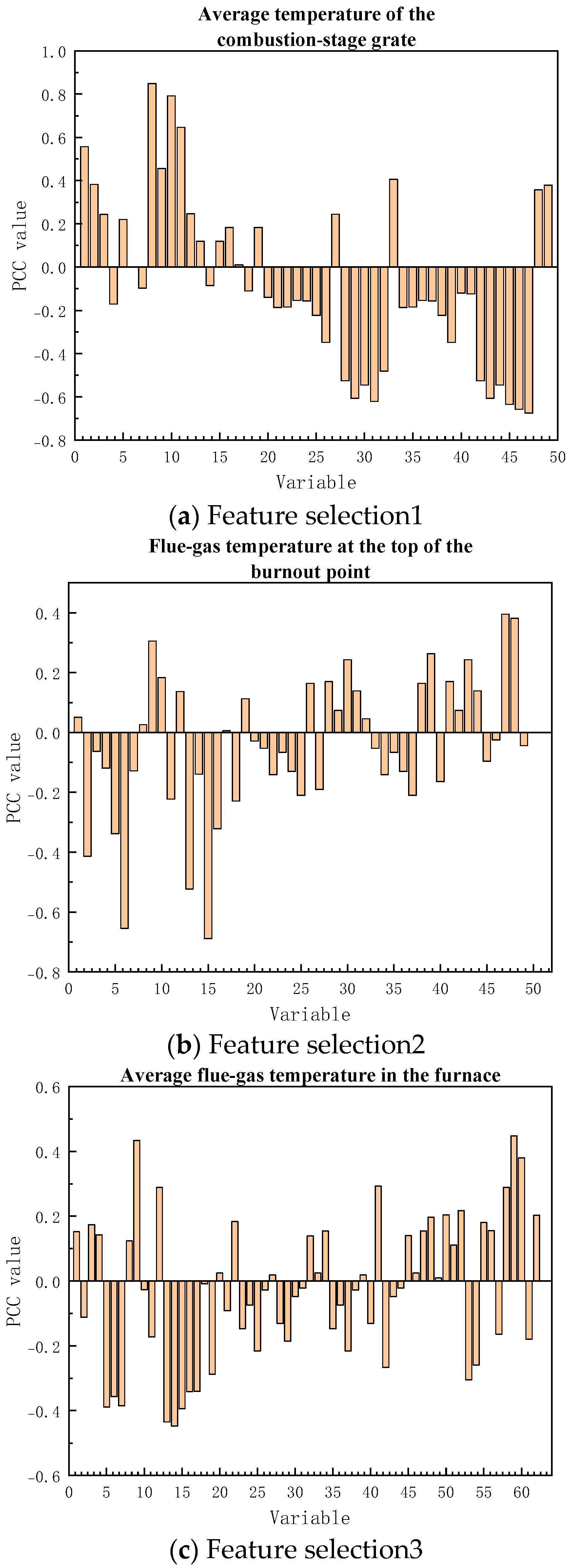
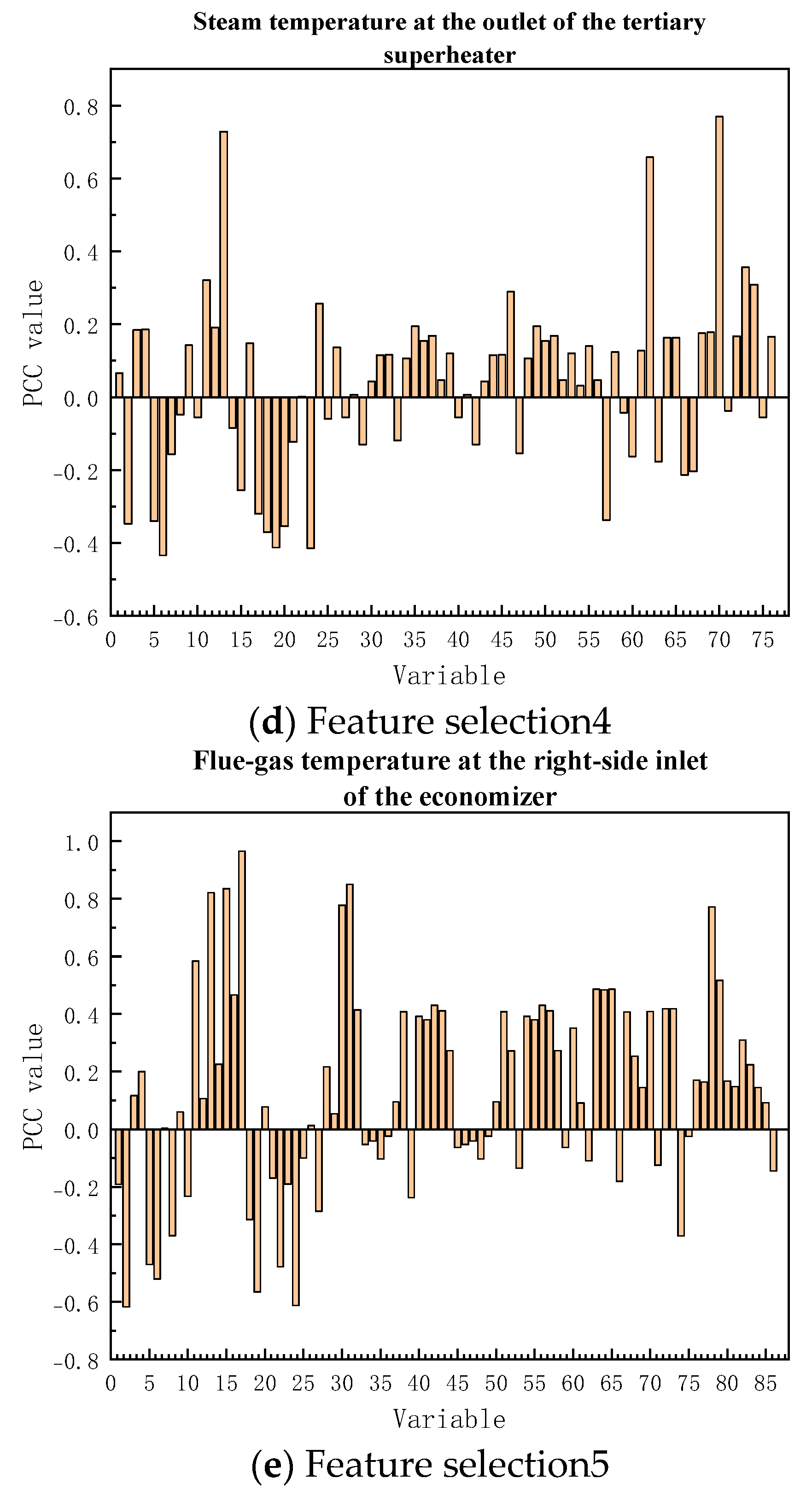
The PCC values of different temperature points and their responding process variables are shown in Table A2 of the Appendix A. The average value θ PCC i ave and the maximum value θ PCC i max are calculated. Taking the step size α = 0.1 to find the optimal threshold, for different regions, the main input variables and correlation values under different thresholds are selected, as shown in Table 1, Table 2, Table 3, Table 4 and Table 5:
In Table 1, the primary air volume is the primary target for combustion control. It determines the amount of available oxygen and directly affects the combustion intensity (temperature) and the waste propulsion speed. The frequency of the primary air fan is the main driving factor. By adjusting the motor speed (frequency), the output capacity of the fan is directly controlled. A higher fan speed means a greater air delivery capacity. The air pressure at the outlet of the primary air fan is the force required for the fan to overcome the system resistance. For the same fan state, an increase in pressure usually drives more air volume through the system. To increase the work of the fan, it is necessary to increase the outlet pressure of the primary air fan and the current of the primary air fan. The air temperature at the outlet of the primary air heater is the temperature that the air reaches after being heated by the heater before entering the incinerator. To provide hot air, it is used for waste drying, combustion support, maintaining stable furnace temperature (especially for MSW with high moisture content and low calorific value), and pollutant control. The air temperature at the inlet of the grate in the combustion section is the initial temperature of the gas participating in the combustion section. High-temperature air carries sensible heat, which can quickly heat the waste, provide the heat required for water evaporation, and promote the release and combustion of volatiles.
In Table 2, the temperature on the left outer side of the furnace wall between the drying section and the combustion section reflects the thermal insulation performance of the refractory material on the inner side of the furnace wall and the intensity of thermal radiation from the combustion section to the furnace wall. An increase in the temperature on the left outer side of the furnace wall indicates the deterioration of the furnace wall’s thermal insulation or an excessively high thermal load in the combustion section, resulting in an increase in heat loss through the furnace wall, which may further lead to a decrease in the flue gas temperature at the burnout point. The outlet temperature of the cooling air on the left side of the furnace wall and the outlet temperature of the cooling air on the left side of the grate both belong to the cooling system, representing the outlet temperature of the cooling air after passing through the interlayer of the furnace wall and the exhaust temperature of the cooling air after passing through the internal channels of the grate, respectively. The increase or decrease in these temperatures can indirectly affect the flue gas temperature at the burnout point.
In Table 3, the temperature at the right slag outlet is the discharge temperature of the slag on the right side of the burnout point. A relatively high slag temperature will cause the temperature of the flue gas to rise before entering the flue, which, in turn, will increase the average temperature of the flue gas in the furnace. The outlet temperature of the secondary air heater is the temperature of the secondary air after heating. The secondary air is a key means to regulate the combustion in the upper part of the furnace. The increase and decrease in its temperature will affect the temperature of the flue gas in the furnace. The outlet temperature of the cooling air on the left side of the furnace wall is the exhaust temperature of the furnace wall cooling system. Its increase and decrease reflect the total heat load in the furnace and can indirectly affect the temperature of the flue gas in the furnace.
In Table 4, the outlet temperature of the cooling air on the right side of the furnace wall reflects the thermal radiation intensity of the furnace on the right side of the combustion section. It can indirectly affect the steam temperature at the outlet of the superheater by influencing the temperature and heat of the flue gas entering the boiler. The air temperature at the outlet of the combustion section is the temperature of the airflow entering the boiler flue after combustion is completed, which can directly affect the tertiary superheater. If this temperature rises 50 °C, the heat transfer efficiency of the tertiary superheater can be increased by 3–5%, and the outlet steam temperature will rise by 8–12 °C. There is a thermal equilibrium relationship between the main steam flow at the boiler outlet and the outlet steam temperature. At the same flue gas temperature, if the steam flow increases, the heat obtained per unit of steam decreases, and the outlet steam temperature rises. An increase in the boiler drum pressure will lead to an increase in the saturated steam temperature, which indirectly causes the outlet steam temperature to rise under the same heat transfer amount.
In Table 5, the flue gas temperature on the right side of the first channel is the initial heat source for all heat transfers in the subsequent flue, which has a direct impact on the flue gas temperature at the right-side inlet of the economizer. The flue gas temperature at the right-side inlet of the protection tube is the temperature when the flue gas enters the superheater protection tube, reflecting the residual heat level after the initial heat absorption of the superheater. If its temperature drops, the flue gas temperature will also drop; there is a heat balance relationship between the main steam output at the boiler outlet and the flue gas temperature at the right-side inlet of the economizer. If the steam output drops, the heat absorption of the boiler decreases, the heat dissipation rate of the flue gas slows down, and the flue gas temperature at the inlet of the economizer rises. The boiler drum pressure and the steam pressure at the outlet of the tertiary superheater have an indirect coupling effect on the flue gas temperature. An increase in the drum pressure causes the flue gas temperature to drop, and an increase in the steam pressure at the outlet of the tertiary superheater causes the flue gas temperature at the inlet of the economizer to rise.
The correlation results between temperature points in different regions and relevant input variables are shown in Figure 4.
Based on the single-temperature-point modeling, a multi-temperature-section model is constructed according to the process characteristics of MSWI. The model system integrates five core temperature monitoring modules of the incineration line, namely average temperature of the combustion-stage grate, flue gas temperature at the top of the burnout point, average flue gas temperature in the furnace, steam temperature at the outlet of the tertiary superheater, and the flue gas temperature at the right-side inlet of the economizer.

3.2.2. Construction Results of the Single-Temperature-Point Model

The selected values of the three hyperparameters of the single-temperature-point model are shown in Table 6. They are obtained using a grid search method with the goal of maximizing the R2 of the validation dataset.
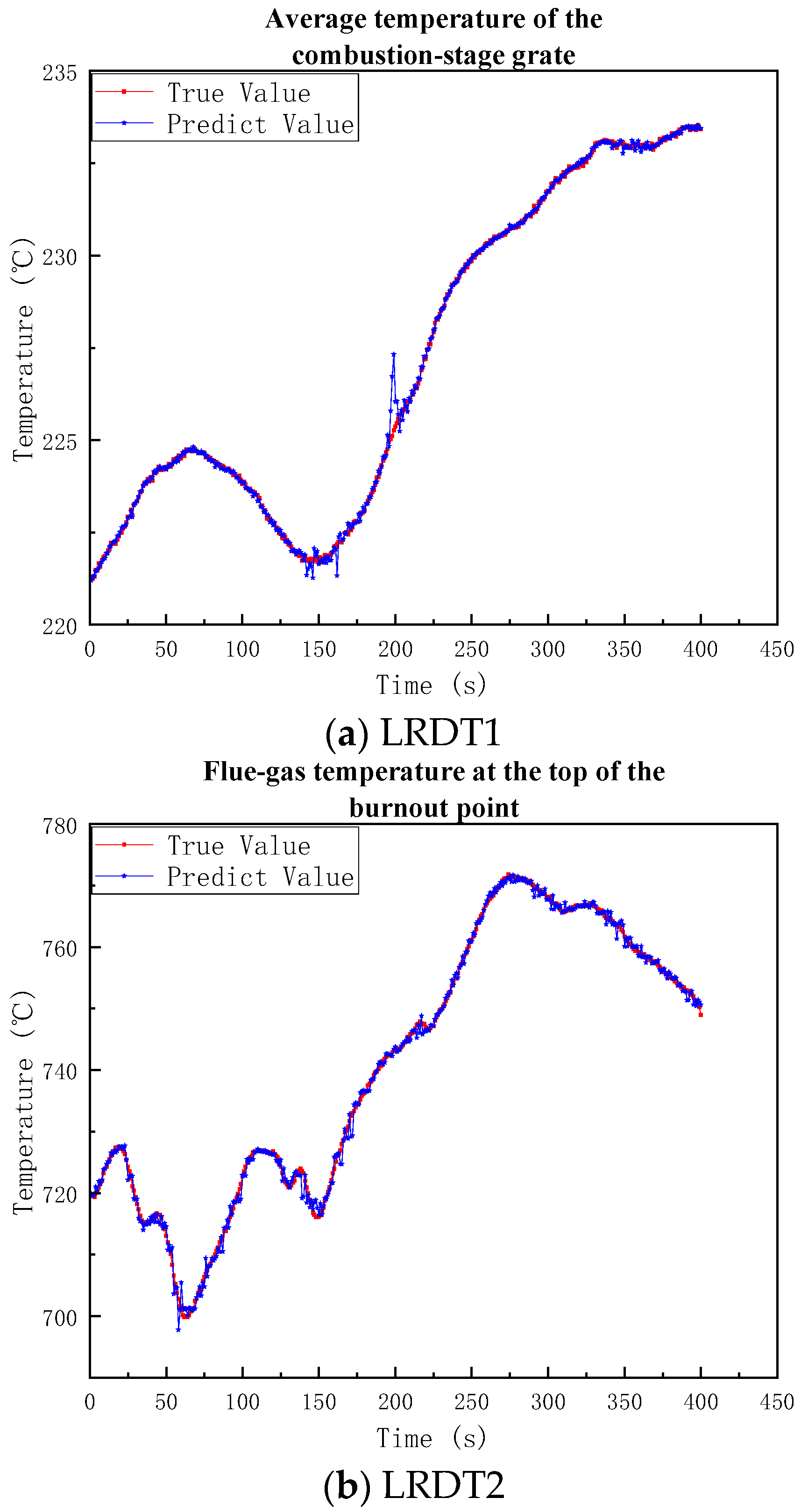
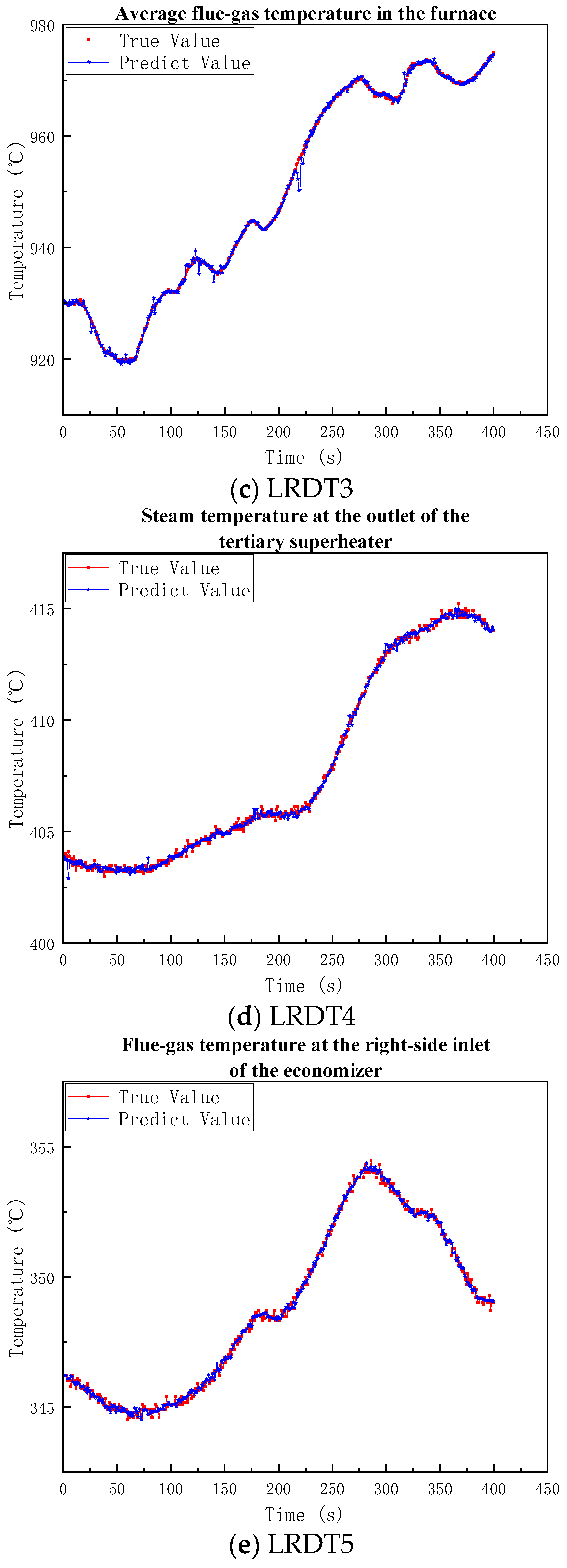
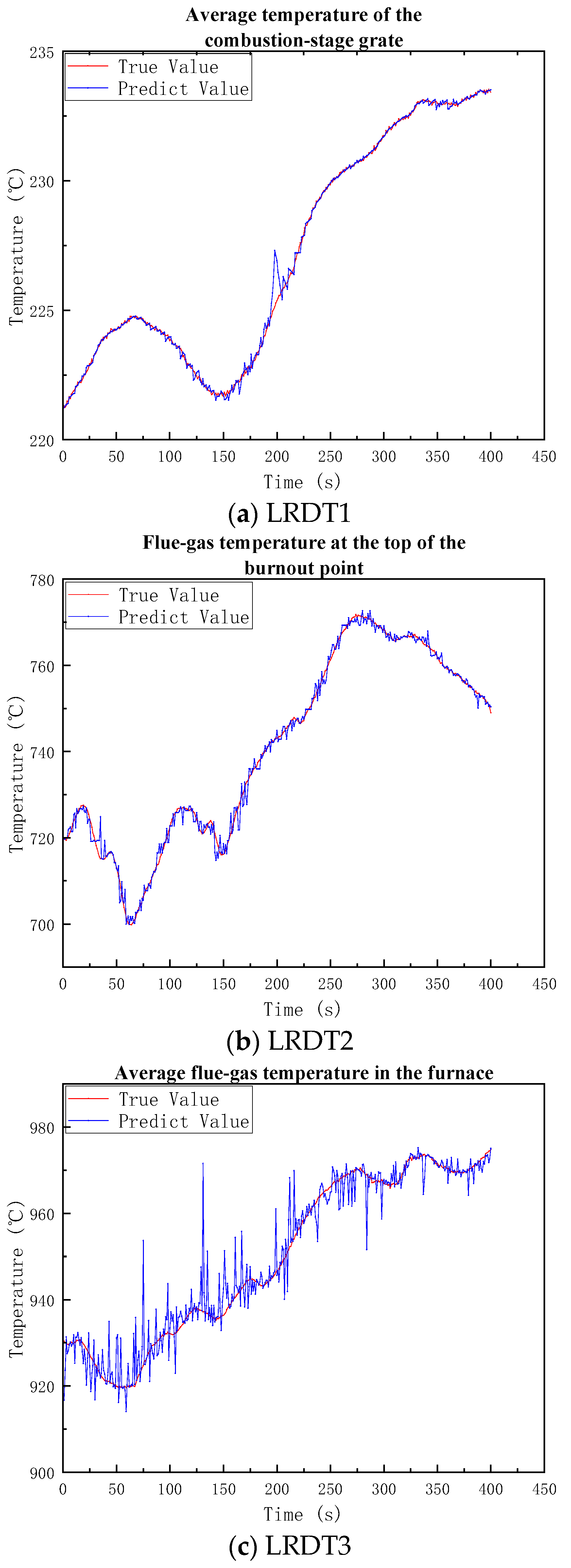
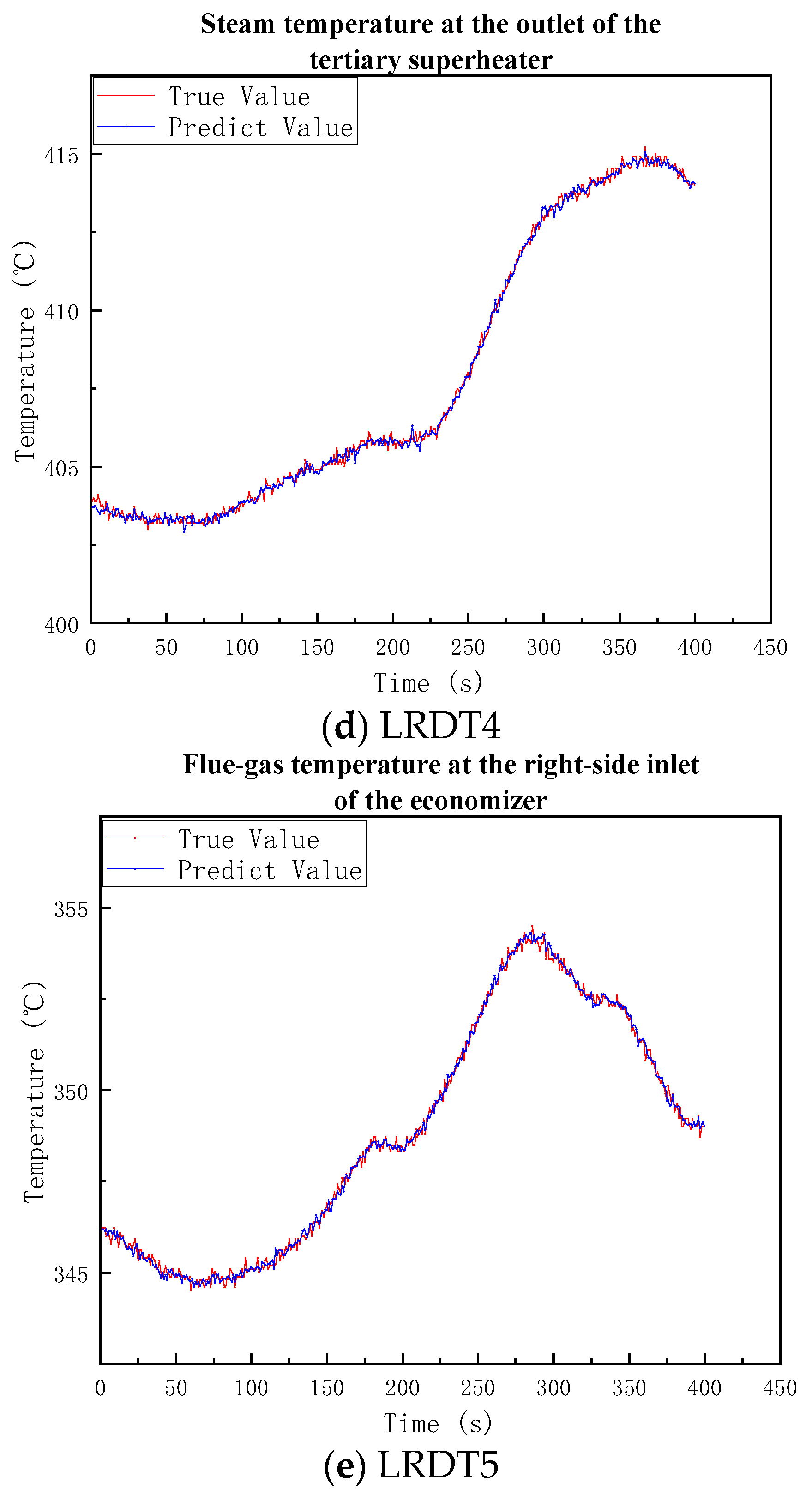
The prediction and statistical results of the five models using the above hyperparameters are shown in Table 7 and Figure 5.
Table 7 and Figure 5 show the following features:
(a) The predicted values of the average grate temperature in the combustion section show high consistency with the actual values in the overall trend. Although relatively large deviations occur at 150 s and 200 s, the overall accuracy is still very high;
(b) The predicted values of the flue gas temperature at the top of the burnout point are highly consistent with the actual values in the overall trend. A minimal lag appears in later-stage predictions during actual value increases, yet accuracy remains high;
(c) The predicted values of the average flue gas temperature in the furnace are very synchronous with the actual values throughout the entire time history, with very few deviations;
(d) Optimal prediction performance occurs for the tertiary superheater outlet steam temperature, achieving precise matching of both steady-state values and dynamic changes;
(e) Prediction accuracy is relatively lower for the economizer’s right-side inlet flue gas temperature.
Therefore, the temperature prediction model demonstrates high accuracy and reliability for single-point temperature prediction. Therefore, an interpretable predictive model for multi-point temperature in MSWI processes has been developed. The process variables contributing to temperature prediction at different points, along with their respective contributions, have been identified. However, it is important to note that, unlike LSTM models, LRDT models do not capture temporal dependency characteristics. Future research should focus on integrating LSTM to overcome the limitations of LRDT models and improve their predictive performance.

3.2.3. Modeling Results of the Multi-Temperature-Point Model

After taking the average of the hyperparameters of the single-temperature-point model, taking the floating values of the regularization coefficient β = 0.001, and the floating values of the minimum number of samples in the leaf nodes γ = 10, the minimum number of samples in the leaf nodes is finally 19, and the regularization coefficient is 0.0027. The statistical and prediction results of different models are shown in Table 8 and Figure 6:
Table 8 and Figure 6 show the following:
(a) The multi-temperature-point model has a low error in the average temperature model of the grate in the combustion section with R2 = 0.9973. The model fits well in this position. The absolute error of the flue gas temperature model at the top of the burnout point is relatively large, with MAE = 1.0473, but R2 = 0.9948 still shows excellent fitting;
(b) The prediction performance of the average flue gas temperature model in the furnace is the worst with R2 = 0.9414. One of the reasons is that two of the input variables of the average flue gas temperature model in the furnace are predicted values. The prediction errors of the first two models have caused noise interference to the prediction of the third model. Even so, the model still captures the overall temperature change law of the primary combustion chamber and has no impact on the subsequent prediction.
(c) The accuracy of the steam temperature model at the outlet of the tertiary superheater is outstanding, and the MSE reaches 0.0278 with R2 = 0.9985. The flue gas temperature model at the right inlet of the economizer performs best in terms of MSE, which is 0.0238.
Therefore, although the prediction of the average flue gas temperature in the furnace by the multi-temperature-point model is distorted due to certain noise interference, it has little impact on the overall prediction accuracy. The comprehensive average performance shows that the model system is generally effective and has high accuracy and engineering credibility for temperature prediction in the combustion and heat transfer processes.

3.3. Method Comparison

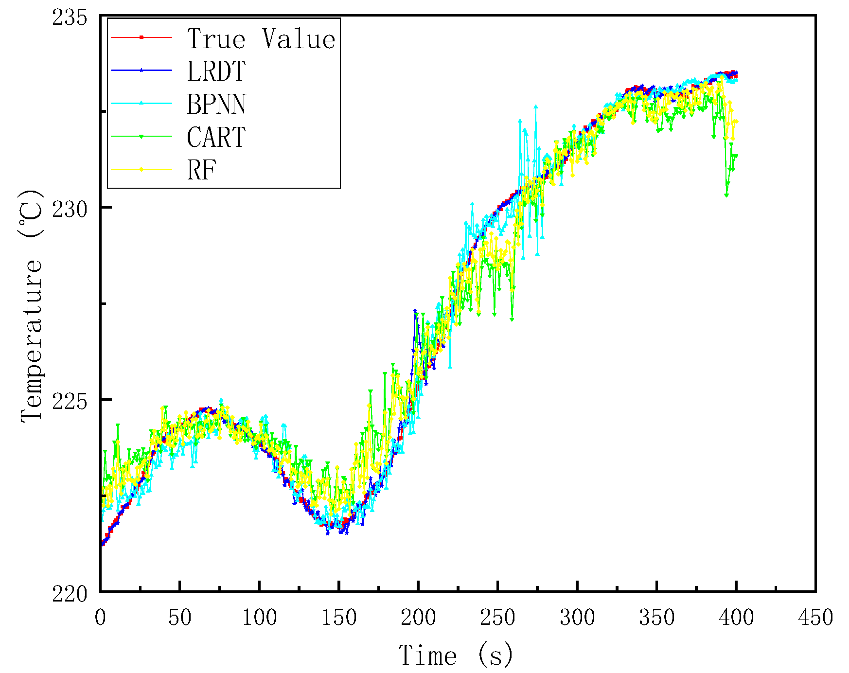
To compare the performance of the models, by taking the prediction of the average grate temperature in the combustion section as an example, this article selects the classification and regression tree (CART), random forest (RF), and back-propagation neural network (BPNN) models to conduct experiments and compares their performance with the proposed method in this article. Among them, CART serves as the foundation of decision trees and a benchmark for interpretability; RF represents the mainstream integrated tree model by adopting the bagging strategy; BPNN, on the other hand, stands for non-tree models (neural networks), and is used to test the robustness and competitiveness of LRDT in cross-paradigm comparisons. This selection ensures a comprehensive evaluation in terms of model complexity, diversity of learning mechanisms, and multi-dimensional performance.
The hyperparameters of the above algorithms are defined as follows. For CART, the minimum number of samples in the leaf nodes is 20, and the number of decision trees is 50. For RF, the minimum number of samples in the leaf nodes is 10, the number of feature selections for each tree is 6, and the number of trees is 100. For BPNN, the maximum number of convergence times is 1500, the number of neurons in the hidden layer is 15, the learning rate is 0.2, the convergence error is 0.001, and the activation function is the tanh function. For LRDT, the minimum number of samples in the leaf nodes is 19, the number of feature selections is 4, and the regularization coefficient is 0.0027. The comparison results are shown in Figure 7.
The comparison of the experimental results between the method proposed in this article and other methods is shown in Table 9. Among them, since the results of BPNN and RF are affected by random parameters, to ensure the fairness of the comparative experiment, the above algorithms are all run 30 times, and the optimal value and the average value are calculated for comparison.
Figure 7 and Table 9 show the following:
(1) The LRDT algorithm shows the optimal performance, with MSE = 0.0503 and MAE = 0.1066 in the testing set, while R2 = 0.9973. This is because it combines the piecewise fitting ability of decision trees and the continuity advantage of linear regression. The dot-line graph shows that the range of its error bars is extremely small, indicating that it can accurately capture the continuous temperature change pattern in the 220–235 °C intervals, with a prediction error of only about 0.1 °C and extremely high stability;
(2) For the BPNN algorithm, the MSE of the testing set is 0.3244 with R2 = 0.9824. Although the light-blue dotted line can track the overall trend, the local fluctuations are obvious, reflecting that the neural network has strong fitting ability through non-linear mapping, but the difference between the best value and the mean value is significant. The model is greatly affected by the random initial weights, and fine-tuning of parameters is required to approach the level of LRDT;
(3) For the CART algorithm, the MSE of the testing set is 0.4932 and the MAE is 0.5203. The green dotted line shows a step-like mutation. Due to the sensitivity of the single-tree structure to noise, overfitting occurs (the best MSE of the training set is 0.2359, which degenerates to 0.4932 in the testing set);
(4) The MSE of the RF algorithm in the testing set is 0.5283, which is the worst. The yellow dotted line deviates significantly from the true value after 300 s. The variance between the validation set and the testing set is smaller than that of CART, indicating that although the ensemble strategy improves the stability, its essential “piecewise constant” prediction characteristic is contrary to the continuous temperature change pattern, resulting in the inability to eliminate the systematic deviation (the best R2 is only 0.9791);
(5) The experiment shows that the LRDT is the best model, with an accuracy of R2 = 0.9967 and MAE = 0.1066.
Therefore, the LRDT algorithm has a good fitting effect and high modeling accuracy in the application of multi-point temperature modeling, meeting the requirements of temperature prediction in actual industrial processes. The experimental results prove the effectiveness of the proposed algorithm.

3.4. Hyperparameter Analysis

To optimize the model performance, a hyperparameter analysis is conducted on the minimum number of samples D best min and the regularization coefficient λ best of the multi-temperature-point model. That is, during the experiment, other hyperparameters are kept at their optimal values, and only the variable to be analyzed is changed. As shown in Table 10, these are the value ranges of each hyperparameter.
(1)
Minimum sample size D best min
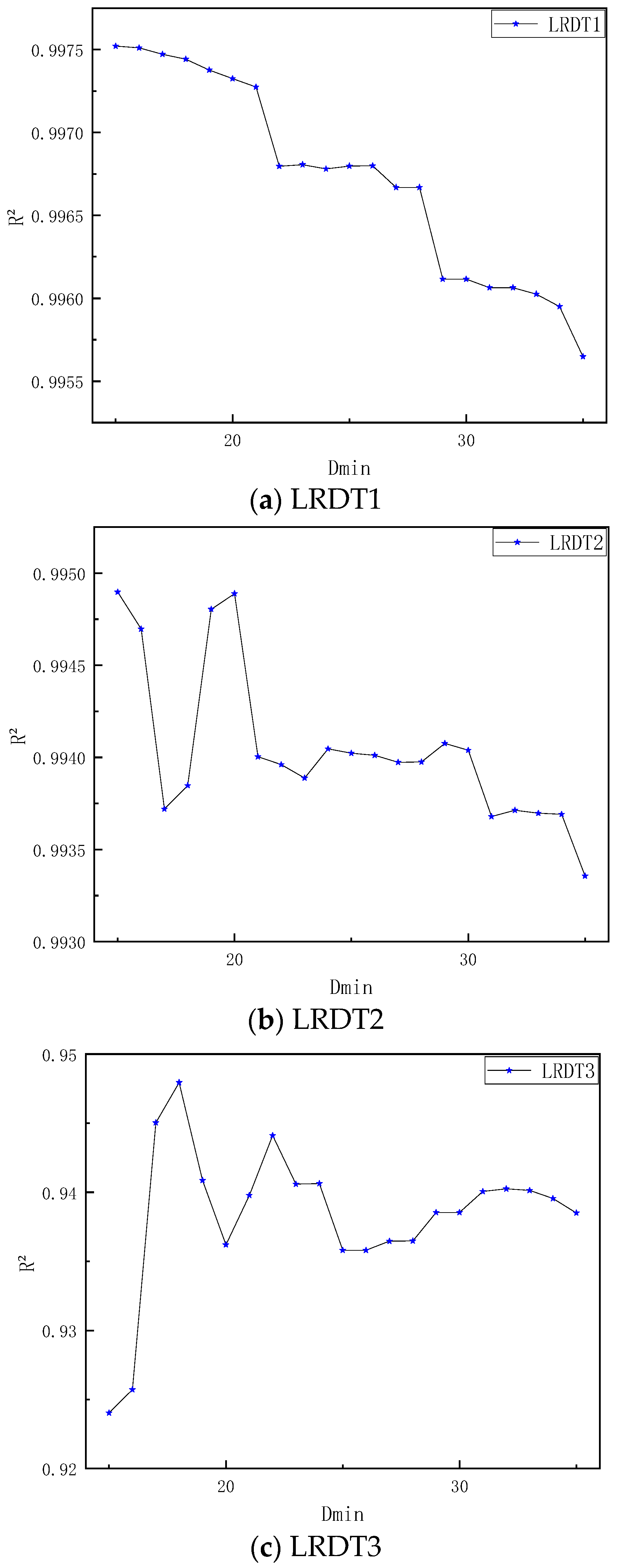
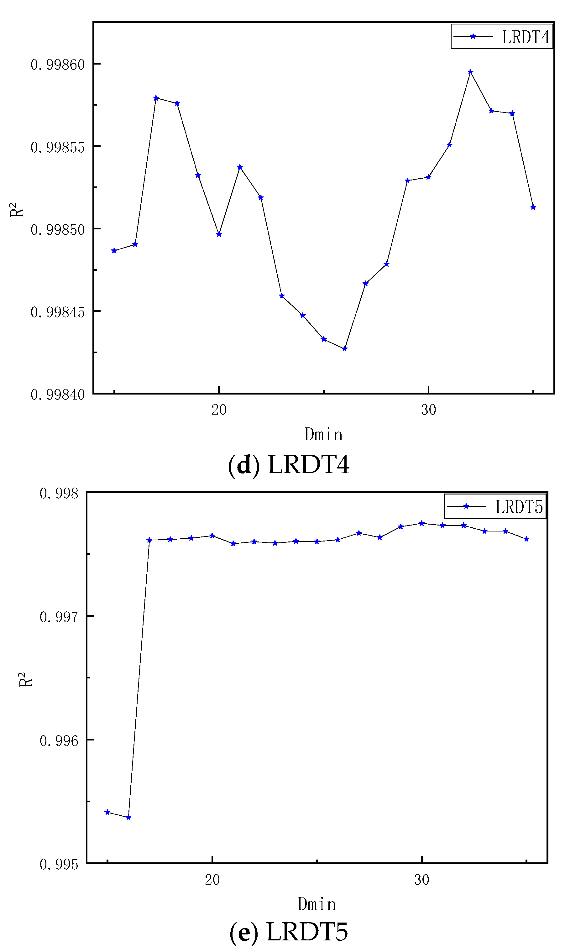
The relationship between the minimum sample size and the multi-temperature-point model R2 is shown in Figure 8.
Figure 8 show the following: (1) The R2 of LRDT 1 monotonically decreases from 0.9975 to 0.9955 as D best min increases; (2) the R2 of LRDT 2 fluctuates violently in the 0.9930–0.9950 interval; (3) the R2 of LRDT 3 fluctuates between 0.92–0.945 and shows a trend of first decreasing and then increasing; (4) the R2 of LRDT 4 fluctuates greatly in the range of 0.9935–0.9986 but rises gently overall; (5) the R2 of LRDT 5 first rises to the peak and then slightly decreases between 0.9950–0.9986, but remains stable at a high level overall (fluctuation range < 0.01).
(2)
Regularization coefficient λ best
The relationship between the regularization coefficient and the multi-temperature-point model R2 is shown in Figure 9.
Figure 9 shows the following: (1) LRDT 1 and LRDT 2 show excellent initial performance in the low regularization region ( λ < 0.0008), providing a high-precision basis for the pre-stage processing of the system; (2) LRDT 3 shows a positive correlation trend, empirically demonstrating the significant improvement effect of regularization on the over-fitting problem of this model; (3) LRDT 4 and LRDT 5 both maintain a high-performance steady state in the λ = 0.001–0.0019 interval, which is due to the efficient ability of their tree structures to capture interaction features. Therefore, there are essential differences in the sensitivity of different models to regularization. LRDT 1 / LRDT 2 are regularization-sensitive types, LRDT 3 is an under-regularization-sensitive type, and LRDT 4 / LRDT 5 have a clear optimal regularization interval.
This diversity indicates that the optimal global hyperparameters of the multi-temperature-point model need to be selected in combination with other hyperparameters.

4. Conclusions

To address the lack of multi-region temperature correlation prediction in the combustion and heat exchange stages of the MSWI process, a method for constructing a multi-point serial temperature prediction model is proposed. The main contributions are as follows: (1) A method for selecting regional features and constructing an interpretable temperature prediction model for multiple single temperature points in multiple regions is proposed, which can fully reflect the contribution of regional features; (2) a method for selecting hyperparameters of the serial-mode multi-point temperature prediction model based on knowledge transfer of multiple single-point temperature models is proposed, which simplifies the complex parameter selection process; (3) a serial-mode multi-point temperature prediction model that conforms to the process mechanism of the combustion and heat exchange stages is constructed, which depicts the coupling mechanism of multiple temperature points and realizes the dynamic correlation modeling of temperature changes in adjacent regions. It effectively solves the problem that traditional single-point prediction models have difficulty in capturing spatial correlations.
The research goal is to develop interpretable predictive models for multiple temperature points, providing valuable insights for future research aimed at maintaining a constant temperature that ensures the stability of the MSWI process and facilitates pollution reduction. The experimental results demonstrate that the proposed multi-point temperature prediction model achieves excellent accuracy and interpretability.
The limitations of this study are evident in the suboptimal selection of hyperparameter values and the need to enhance the model’s adaptability to dynamic MSWI processes. In future work, intelligent optimization algorithms are to be employed to achieve efficient and automated hyperparameter tuning. Additionally, an operating conditions drift detection method is to be addressed to continuously monitor changes in the modeling data distribution and to identify new samples that can represent the concept drift to update the proposed multi-point serial temperature prediction model. This approach can significantly enhance the model’s adaptability to time-varying conditions, ensuring its prediction accuracy and long-term robustness in dynamic environments.

Author Contributions

Conceptualization, W.W. and J.T.; methodology, W.W. and J.T.; software, Y.Z. and J.R.; validation, J.R.; investigation, Y.Z.; resources, Y.Z. and J.R.; data curation, Y.Z.; writing—review and editing, W.W. and J.T.; visualization, Y.Z.; supervision, W.W. and J.T.; project administration, W.W. and J.T. All authors have read and agreed to the published version of the manuscript.

Funding

This work was supported in part by the General Scientific Research Projects of Liaoning Province Science and Technology Joint Plan Project under Grant 2024JH2/102600083, and in part by Liaoning Provincial Department of Education under Grant JYTMS20230489.

Institutional Review Board Statement

Not applicable.

Informed Consent Statement

Not applicable.

Data Availability Statement

The data presented in this study are available on request from the corresponding author.

Conflicts of Interest

The authors declare no conflict of interest.

Appendix A

Table A1. Symbols used in this article and their meanings.
NumSymbolActual Meaning
1. X ori 1 , X ori 2 , X ori 3 , X ori 4 , X ori 5 Original dataset located at the grate in the combustion section, the grate in the burnout section, the flue gas in the furnace, the high-temperature heat exchange zone, and the low-temperature heat exchange zone and in front of them, respectively, during the MSWI process
2. X sel 1 , X sel 2 , X sel 3 , X sel 4 , X sel 5 The input data of the average temperature of the combustion-stage grate, flue gas temperature at the top of the burnout point, average flue gas temperature in the furnace, steam temperature at the outlet of the tertiary superheater, and the flue gas temperature at the right-side inlet of the economizer, respectively, after correlation selection
3. LRDT 1 ini , LRDT 2 ini , LRDT 3 ini , LRDT 4 ini , LRDT 5 ini Initial model of the grate in the combustion section, the top of the burnout point, average flue gas temperature, high-temperature heat exchange zone, and low-temperature heat exchange zone, respectively
4. LRDT 1 , LRDT 2 , LRDT 3 , LRDT 4 , LRDT 5 Model of the grate in the combustion section, the top of the burnout point, average flue gas temperature, high-temperature heat exchange zone, and low-temperature heat exchange zone, respectively
5. y ^ 1 , y ^ 2 , y ^ 3 , y ^ 4 , y ^ 5 Predicted value of the model of the grate in the combustion section, the top of the burnout point, average flue gas temperature, high-temperature heat exchange zone, and low-temperature heat exchange zone, respectively
6. H sin gle i Optimal hyperparameter set of the i-th LRDT model
7. H sin gle 1 , H sin gle 2 , H sin gle 3 , H sin gle 4 , H sin gle 5 Optimal hyperparameter set of LRDT 1 , LRDT 2 , LRDT 3 , LRDT 4 , and LRDT 5 , respectively
8. H multi Global optimal hyperparameter
9. ( r i p i ) i Correlation coefficient of the p -th feature in x ori i of the i -th model
10. θ PCC i max Maximum value of threshold calculation for the i -th feature selection module
11. θ PCC i ave Average value of the threshold calculation for the i -th feature selection module
12. α Optimization step size for the correlation coefficient threshold
13. θ i Optimal threshold of the i -th model
14. X input i Input of the i -th model
15. D i L Left child node after dataset partitioning
16. D i R Right child node after dataset partitioning
17. φ nonleaf 1 Indicator function for partitioning the dataset into left and right child nodes
18. x n i m s The m s -th feature value of the n i -th sample
19. x nonleaf 1 Node judge of the first non-leaf node
20. Ω l ( n i , m s ) MSE value after splitting the dataset into D i L and D i R under the current traversal
21. ( n i , m s ) Dataset coordinates
22. f MSE ( · ) Solving function for MSE
23. L i Maximum number of traversals
24. D i min Minimum number of samples in the i -th model
25. X sel i Input data of the i -th LRDT model
26. λ i Regularization coefficient of the i -th model
27. M i Number of features in the i -th model
28. λ best Optimal regularization term coefficient
29. D best min Optimal minimum number of samples
30. M ave Average number of features
31. N Number of samples in the dataset
32. w i leaf k Weight vector of the leaf node under the k -th path
33. X k Input data under the k -th path
34. y i k Temperature vector of the i -th temperature point under the k -th path
35. N k Number of samples of X i k
36. M k Number of features of X i k
37. D i k Input characteristics of the k -th path
38. y ^ i k Predicted output of leaf nodes under the k -th path
39. β Upper and lower floating values for optimizing the average regularization term coefficient
40. γ Upper and lower floating values for optimizing the average minimum number of samples
41. y i k n Output of leaf nodes under the k -th path of the n -th sample at the i -th temperature point
42. X i k n Input data under the k -th path of the n -th sample at the i -th temperature point
43. w i leaf k n Weight vector under the k -th path of the n -th sample at the i -th temperature point
Table A2. PCC values of different temperature points and their corresponding process variables.
(a) The average temperature of the combustion-stage grate
NumVariable NameUnitPCC Value
1.Temperature on the left of the slag outlet°C0.8495
2.Air temperature at the outlet of the primary air heater (combustion 2-2 + afterburning)°C0.7928
3.Air temperature at the inlet of the combustion section grate (combustion 1-1, 2 + 2-1)°C0.6467
4.Temperature of the left inner side of the drying section grate°C0.5576
5.Temperature on the right of the slag outlet°C0.4560
6.Right afterburning grate (air volume setting) km 3 N / h 0.4063
7.Temperature of the left outer side of the drying section grate°C0.3832
8.Current of the grate cooling fanA0.3789
9.Current of the furnace wall cooling fanA0.3572
10.Air temperature at the inlet of the drying section grate°C0.2469
11.Right drying grate 1 (air volume setting) km 3 N / h 0.2444
12.Temperature of the right inner side of the drying section grate°C0.2437
13.Temperature of the left inner side of the furnace wall between the drying section and the combustion section grates°C0.2205
14.Biogas flow rate in the drying section m 3 / h 0.1837
15.Temperature of the cooling air outlet on the right side of the grate°C0.1831
16.Temperature of the cooling air outlet on the left side of the grate°C0.1196
17.Temperature of the cooling air outlet on the left side of the furnace wall°C0.1194
18.Air temperature at the outlet of the drying section°C0.0103
19.Temperature of the left outer side of the furnace wall between the drying section and the combustion section grates°C0.0002
20.Frequency of the primary fanHz−0.6754
21.Current of the primary fanA−0.6587
22.Air pressure at the outlet of the primary fan KPa −0.6354
23.Right combustion grate 2-1 (air volume setting) km 3 N / h −0.6221
24.Right combustion grate 1-1 (air volume setting) km 3 N / h −0.6080
25.Air flow in the right 2-1 section of the combustion-stage grate km 3 N / h −0.6080
26.Right combustion grate 1-2 (air volume setting) km 3 N / h −0.5455
27.Air flow in the left 2-2 section of the combustion-stage grate km 3 N / h −0.5454
28.Right drying grate 2 (air volume setting) km 3 N / h −0.5258
29.Air flow rate of the left 2-1 section of the combustion section grate km 3 N / h −0.5258
30.Right combustion grate 2-2 (air volume setting) km 3 N / h −0.4812
31.Left combustion grate 2-2 (air volume setting) km 3 N / h −0.3493
32.Air flow rate of the right 1-1 section of the combustion section grate km 3 N / h −0.3493
33.Left combustion grate 2-1 (air volume setting) km 3 N / h −0.2234
34.Air flow rate of the left 1-1 section of the combustion section grate km 3 N / h −0.2234
35.Left drying grate 1 (air volume setting) km 3 N / h −0.1875
36.Air flow rate of the left drying grate 1 km 3 N / h −0.1875
37.Left drying grate 2 (air volume setting) km 3 N / h −0.1849
38.Air flow rate of the right drying grate 1 km 3 N / h −0.1849
39.Temperature of the right outer side of the drying section grate°C−0.1711
40.Left combustion grate 1-2 (air volume setting) km 3 N / h −0.1565
41.Air flow rate of the right drying grate 2 km 3 N / h −0.1565
42.Left combustion grate 1-1 (air volume setting) km 3 N / h −0.1546
43.Air flow rate of the left drying grate 2 km 3 N / h −0.1546
44.Biogas flow rate in the combustion section m 3 / h −0.1406
45.Air flow rate of the right 1-2 section of the combustion section grate km 3 N / h −0.1235
46.Air flow rate of the left 1-2 section of the combustion section grate km 3 N / h −0.1196
47.Air temperature at the outlet of the combustion section°C−0.1109
48.Temperature of the right outer side of the furnace wall between the drying section and the combustion section grates°C−0.0974
49.Temperature of the cooling air outlet on the right side of the furnace wall°C−0.0850
(b) Flue gastemperature at the top of the burnout point
NumVariable nameUnitPCC value
1.Current of the furnace wall cooling fanA0.3948
2.Current of the grate cooling fanA0.3819
3.Temperature at the right of the slag outlet°C0.3048
4.Air flow of left section 1-2 of the combustion-stage grate km 3 N / h 0.2635
5.Air flow of left section 2-2 of the combustion-stage grate km 3 N / h 0.2425
6.Right combustion grate 1-2 (air volume setting) km 3 N / h 0.2424
7.Air temperature at the outlet of the primary air heater (combustion 2-2 + afterburning)°C0.1831
8.Air flow of left section 2-1 of the combustion-stage grate km 3 N / h 0.1702
9.Right drying grate 2 (air volume setting) km 3 N / h 0.1701
10.Left combustion grate 2-2 (air volume setting) km 3 N / h 0.1640
11.Air flow of right section 1-1 of the combustion-stage grate km 3 N / h 0.1639
12.Right combustion grate 2-1 (air volume setting) km 3 N / h 0.1392
13.Air flow of right section 2-2 of the combustion-stage grate km 3 N / h 0.1391
14.Air temperature at the inlet of the drying section grate°C0.1368
15.Biogas flow rate in the drying section m 3 / h 0.1126
16.Right combustion grate 1-1 (air volume setting) km 3 N / h 0.0733
17.Air flow of right section 2-1 of the combustion-stage grate km 3 N / h 0.0732
18.Temperature at the left inner side of the drying section grate°C0.0508
19.Right combustion grate 2-2 (air volume setting) km 3 N / h 0.0459
20.Temperature at the left of the slag outlet°C0.0256
21.Air temperature at the outlet of the drying section°C0.0060
22.Temperature of the cooling air outlet on the left side of the grate°C−0.6889
23.Temperature at the left outer side of the furnace wall between the drying section and the combustion section grates°C−0.6545
24.Temperature of the cooling air outlet on the left side of the furnace wall°C−0.5226
25.Temperature at the left outer side of the drying section grate°C−0.4137
26.Temperature at the left inner side of the furnace wall between the drying section and the combustion section grates°C−0.3379
27.Temperature of the cooling air outlet on the right side of the grate°C−0.3216
28.Air temperature at the outlet of the combustion section°C−0.2295
29.Air temperature at the inlet of the combustion section grate (combustion 1-1, 2 + 2-1)°C−0.2227
30.Left combustion grate 2-1 (air volume setting) km 3 N / h −0.2102
31.Air flow of left section 1-1 of the combustion-stage grate km 3 N / h −0.2102
32.Right drying grate 1 (air volume setting) km 3 N / h −0.1907
33.Air flow of right section 1-2 of the combustion-stage grate km 3 N / h −0.1642
34.Left drying grate 2 (air volume setting) km 3 N / h −0.1409
35.Air flow of right 1 of the drying grate km 3 N / h −0.1409
36.Temperature of the cooling air outlet on the right side of the furnace wall°C−0.1395
37.Left combustion grate 1-2 (air volume setting) km 3 N / h −0.1305
38.Air flow of right 2 of the drying grate km 3 N / h −0.1305
39.Temperature at the right outer side of the furnace wall between the drying section and the combustion section grates°C−0.1287
40.Temperature at the right outer side of the drying section grate°C−0.1193
41.Air pressure at the outlet of primary air fan KPa −0.0962
42.Left combustion grate 1-1 (air volume setting) km 3 N / h −0.0671
43.Air flow of left 2 of the drying grate km 3 N / h −0.0671
44.Temperature at the right inner side of the drying section grate°C−0.0634
45.Left drying grate 1 (air volume setting) km 3 N / h −0.0528
46.Air flow of left 1 of the drying grate km 3 N / h −0.0528
47.Frequency of the primary air fan Hz −0.0440
48.Biogas flow rate in the combustion section m 3 / h −0.0284
49.Current of the primary air fanA−0.0251
(c) Average flue gas temperature in the furnace
NumVariable nameUnitPCC value
1.Current of the furnace wall cooling fanA0.4477
2.Current of the grate cooling fanA0.3799
3.Air flow rate of left section 1-2 of the combustion section grate km 3 N / h 0.2927
4.Air temperature at the inlet of the drying section grate°C0.2887
5.Current of the secondary fanA0.2886
6.Cumulative urea solution volume of furnace 2, SL0.2175
7.Secondary air flow rate km 3 N / h 0.2045
8.Secondary air fan frequency Hz 0.2027
9.Air flow rate of the right grate in the burnout section km 3 N / h 0.1971
10.Cumulative primary air volume of furnace 2 km 3 N 0.1830
11.Air pressure at the outlet of the secondary fanKPa0.1806
12.Furnace negative pressure Pa 0.1555
13.Air flow rate of the left grate in the burnout section km 3 N / h 0.1546
14.Air flow rate of left section 2-2 of the combustion section grate km 3 N / h 0.1395
15.Flow rate of branch 1 of the secondary fan km 3 N / h 0.1113
16.Air flow rate of right section 2-2 of the combustion section grate km 3 N / h 0.0247
17.Air flow rate of left section 1-1 of the combustion section grate km 3 N / h 0.0184
18.Cumulative secondary air volume of furnace 2 km 3 N 0.0105
19.Temperature of the cooling air outlet on the left side of the furnace wall°C−0.4472
20.Air temperature at the outlet of the secondary air heater°C−0.4342
21.Temperature of the cooling air outlet on the right side of the furnace wall°C−0.3942
22.Temperature of the cooling air outlet on the left side of the grate°C−0.3415
23.Temperature of the cooling air outlet on the right side of the grate°C−0.3410
24.Amount of urea diluent injected into the furnaceL/h−0.3049
25.Air flow rate of right section 1-2 of the combustion section grate km 3 N / h −0.2658
26.Air pressure at the outlet of the primary fan KPa −0.2596
27.Air flow rate of left drying grate 2 km 3 N / h −0.2156
28.Frequency of the primary fan Hz −0.1800
29.Current of the primary fanA−0.1644
30.Air flow rate of left drying grate 1 km 3 N / h −0.1471
31.Air flow rate of right section 1-1 of the combustion section grate km 3 N / h −0.1311
32.Air flow rate of right drying grate 1 km 3 N / h −0.0746
33.Air flow rate of left section 2-1 of the combustion section grate km 3 N / h −0.0484
34.Air flow rate of right drying grate 2 km 3 N / h −0.0281
35.Air flow rate of right section 2-1 of the combustion section grate km 3 N / h −0.0214
(d) Steam temperature at the outlet of the tertiary superheater
NumVariable nameUnitPCC value
1.Boiler drum pressureMPa0.7696
2.Flue gas temperature at the right inlet of the protection tube°C0.7286
3.Main steam volume at the boiler outlett/h0.6584
4.Flue gas temperature on the right side of the first channel°C0.3205
5.Flue gas temperature at the left inlet of the protection tube°C0.1905
6.Accumulated main steam volume of the boilert0.1275
7.Accumulated cooling water flow of the primary superheatert0.1240
8.Cooling water flow of the primary superheatert/h−0.3371
9.Total desuperheating water of the primary and secondary superheaterst/h−0.1632
10.Flue gas temperature on the left side of the first channel°C−0.0557
11.Cooling water flow of the secondary superheatert/h−0.0426
(e) Flue gas temperature at the right-side inlet of the economizer
NumVariable nameUnitPCC value
1.Flue gas temperature at the right inlet of the evaporator°C0.9660
2.Feed water flow of economizer No. 2t/h0.4865
3.Feed water flow of economizer No. 1t/h0.4847
4.Flue gas temperature at the left inlet of the evaporator°C0.4659
5.Flow of secondary fan branch 1 km 3 N / h 0.0908
6.Total feed water volume of the economizert/h−0.1099

References

  1. Tang, J.; Xia, H.; Yu, W.; Qiao, J. Research Status and Prospect of Intelligent Optimization Control of Municipal Solid Waste Incineration Process. Acta Autom. Sin. 2023, 49, 2019–2059. [Google Scholar] [CrossRef]
  2. Chen, A.; Chen, J.; Cui, J.; Fan, C.; Han, W. Research on the Risk and Countermeasures of “Garbage Surrounding Cities” in 31 Provincial Capital Cities in China—An Empirical Study Based on the DIIS Method. Bull. Chin. Acad. Sci. 2019, 34, 797–806. [Google Scholar] [CrossRef]
  3. Xu, H. Current Situation, Pollution Causes and Governance Countermeasures of Municipal Solid Waste. Resour. Conserv. Environ. 2022, 250, 39–42. [Google Scholar] [CrossRef]
  4. Liu, S. Research on Treatment and Utilization of Municipal Solid Waste. Leather Mak. Environ. Technol. 2022, 3, 173–175. [Google Scholar] [CrossRef]
  5. Jiang, Z.; Xu, J. Research on Solid Waste Treatment and Resource Utilization under the Background of “Waste-Free City”. China Resour. Compr. Util. 2023, 41, 70–72. [Google Scholar]
  6. Pan, Y. Treatment and Resource Utilization of Municipal Solid Waste. Leather Mak. Environ. Technol. 2021, 2, 103–105. [Google Scholar]
  7. Liu, H.; Wang, H. The Optimal Technical Path for Low-Carbon and Environmentally Friendly Treatment of Municipal Domestic Garbage in County-Level Areas—Preparation of Solid Recovery Fuel. Green Metall. 2023, 39, 90–94+100. [Google Scholar] [CrossRef]
  8. Zhou, B.; Bai, L. Technology for Domestic Waste Incineration Treatment, 1st ed.; Chemical Industry Press: Shanghai, China, 2024; ISBN 978-7-122-44651-0. [Google Scholar]
  9. Song, X.; Min, H.; Zhao, L.; Fu, Q.; Zheng, W.; Wang, X.; Ding, X.; Liu, L.; Ji, M. The Experience and Development of the Treatment Technology of Municipal Solid Waste Leachate in China. Water 2022, 14, 2458. [Google Scholar] [CrossRef]
  10. Zou, C.; He, D. Waste to Treasure: Recycling Solid Waste. Yantai Daily, 29 May 2023. [Google Scholar] [CrossRef]
  11. Guo, X.; Hu, J.; Wang, C. Ultrasonic-Assisted Hydrothermal Synthesis Autoclaved Bricks from Municipal Solid Waste Incineration Fly Ash and Coal Fly Ash (MSWI-FA). J. Wuhan Univ. Technol.-Mat. Sci. Edit. 2025, 40, 439–448. [Google Scholar] [CrossRef]
  12. Joumblat, R.; Al Basiouni Al Masri, Z.; Elkordi, A. Dynamic Modulus and Phase Angle of Asphalt Concrete Mixtures Containing Municipal Solid Waste Incinerated Fly Ash as Mineral Filler Substitution. Int. J. Pavement Res. Technol. 2023, 16, 1196–1216. [Google Scholar] [CrossRef]
  13. Hu, C.; Lou, X.; Liu, D. Analysis of Municipal Solid Waste Status and Governance Countermeasures. Leather Mak. Environ. Technol. 2023, 4, 83–85. [Google Scholar] [CrossRef]
  14. Yao, W. Research on Comprehensive Treatment Technology of Municipal Solid Waste. Resour. Conserv. Environ. 2019, 212, 89. [Google Scholar] [CrossRef]
  15. Zhang, F Research on Municipal Solid Waste Comprehensive Disposal in the Low-Carbon Era. China Resour. Compr. Util. 2022, 40, 173–175.
  16. Ye, L.; Liu, L.; Chen, W. Exploring the Current Status and Development Trends of Municipal Solid Waste Treatment Technology. Shihezi Sci. Technol. 2022, 6, 48–49. [Google Scholar]
  17. Chen, J.; Li, W.; Li, Y. Effect of entrained flow bed gasification fine slag on melting temperature and harmlessness of municipal solid waste incineration fly ash. Coal Convers. 2025, 48, 101–110. [Google Scholar] [CrossRef]
  18. Zhang, L.J.; Zhang, R.; Liu, D. Full-process simulation and evaluation analysis of coal-coupled waste incineration power generation system. Clean Coal Technol. 2023, 29, 109–116. [Google Scholar]
  19. Qiao, J.; Huang, W.; Ding, H.; Yu, T. Research on Feature Modeling Methods and Applications for Complex Industrial Processes. Control Decis. 2023, 38, 2063–2078. [Google Scholar] [CrossRef]
  20. Li, B.; Chen, N.; Luo, B.; Chen, J.; Yang, C.; Gui, W. ADP-Based Event-Triggered Constrained Optimal Control on Spatiotemporal Process: Application to Temperature Field in Roller Kiln. IEEE Trans. Neural Netw. Learn. Syst. 2024, 35, 3229–3241. [Google Scholar] [CrossRef]
  21. Zhu, H.; He, Z.; Han, X.; Li, J.; Dong, X.; Qiao, S.; Yu, X.; Zhao, Y. Establishment and Application of Temperature Prediction Model for Alloying Steel Liquid during Converter Outgoing Steel. J. Iron Steel Res. 2025, 37, 751–760. [Google Scholar] [CrossRef]
  22. Chen, F.; Yang, M.; Yan, W. Data-Driven Prognostic Model for Temperature Field in Additive Manufacturing Based on the High-Fidelity Thermal-Fluid Flow Simulation. Comput. Methods Appl. Mech. Eng. 2022, 392, 114652. [Google Scholar] [CrossRef]
  23. Sun, S.; Du, J.; Peng, G.; Yang, N. A Data-Driven Method to Construct Prediction Model of Solar Stills. Desalination 2024, 587, 117946. [Google Scholar] [CrossRef]
  24. Wang, Y.; Ma, H.; Zeng, W.; Bu, Q.; Yang, X. Influence of Moisture Content and Inlet Temperature on the Incineration Characteristics of Municipal Solid Waste (MSW). Appl. Therm. Eng. 2025, 258, 124677. [Google Scholar] [CrossRef]
  25. Qais, M.H.; Loo, K.H.; Lai, C.-M. Gated Recurrent Unit-Based Data-Driven Model for Predicting Pot Temperature in Induction Cooking Systems. Therm. Sci. Eng. Prog. 2024, 50, 102526. [Google Scholar] [CrossRef]
  26. Tang, J.; Zhuang, J.; Qiao, J. Numerical Simulation and Analysis of Municipal Solid Waste Incineration Process in Furnace. Control Eng. 2022, 29, 1921–1927. [Google Scholar] [CrossRef]
  27. Jian, J.; Sun, A.; Tang, J. Data-Driven Prediction of Furnace Temperature in Municipal Solid Waste Incineration Process. Control Eng. 2024, 1–10. [Google Scholar] [CrossRef]
  28. Yan, A.; Wang, R.; Guo, J.; Tang, J. A Knowledge Transfer Online Stochastic Configuration Network-Based Prediction Model for Furnace Temperature in a Municipal Solid Waste Incineration Process. Expert Syst. Appl. 2024, 243, 122733. [Google Scholar] [CrossRef]
  29. Peng, C.; Lan, Y.; Zou, C.; Cai, L. Optimized Random Forest (GA-RF) Model for Predicting Ignition Temperature of Coal Powder in Oxygen-Enriched Combustion. Clean Coal Technol. 2020, 26, 71–76. [Google Scholar] [CrossRef]
  30. Wang, Y.; Lei, Y. Prediction of Main Steam Temperature in Garbage Incineration Boiler Based on DCS Data and Combustion Image. Proc. CSEE 2023, 43, 8790–8801. [Google Scholar] [CrossRef]
  31. Xu, L.; Zhu, S.; Yao, J.; Guan, H. Temperature Prediction of Plate Heat Exchanger Based on Kriging Model. J. Nat. Sci. NanJing Univ. Sci. Technol. 2025, 23, 27–35. [Google Scholar] [CrossRef]
  32. Wu, J.; Liu, H.; Lan, J. Review of Resource Utilization Methods for Municipal Domestic Garbage. China Sci. Technol. Inf. 2011, 5, 27–28. [Google Scholar]
  33. Ying, S.; Peng, Y.; Zhang, C.; Ding, J.; Zhu, Z.; Sun, S.; Zhao, X.; Lu, S. Influence of Chlorine Removal and CaO Addition on Low-Temperature Pyrolysis of PCDD/Fs in MSWI Fly Ash. J. Environ. Chem. Eng. 2025, 13, 116873. [Google Scholar] [CrossRef]
  34. He, S.; Zhou, Y.; Yu, P.; Xia, X.; Yang, H. Effects and Mechanism of the Conditions of Sintering on Heavy Metal Leaching Characteristic in Municipal Solid Waste Incineration Fly Ash. Environ. Sci. Pollut. Res. 2022, 29, 84886–84902. [Google Scholar] [CrossRef] [PubMed]
  35. Fan, X.; Zhou, Z.; Huang, B.; Ji, Z.; Gan, M.; Sun, Z.; Chen, X.; Huang, X.; Wang, G. Emission Characteristics and Control Technology of Heavy Metals during Collaborative Treatment of Municipal Solid Waste Incineration Fly Ash in Iron Ore Sintering Process. J. Iron Steel Res. Int. 2024, 31, 2655–2663. [Google Scholar] [CrossRef]
  36. Liu, X.; Duan, Y.; Zheng, L.; Long, L.; Khalid, Z.; Huang, Q.; Jiang, X. High-Temperature Corrosion Mechanism Analysis of 310S Alloy in Typical MSWI Flue Gas Environment at 460–580 °C. J. Mater. Cycles Waste Manag. 2024, 26, 197–212. [Google Scholar] [CrossRef]
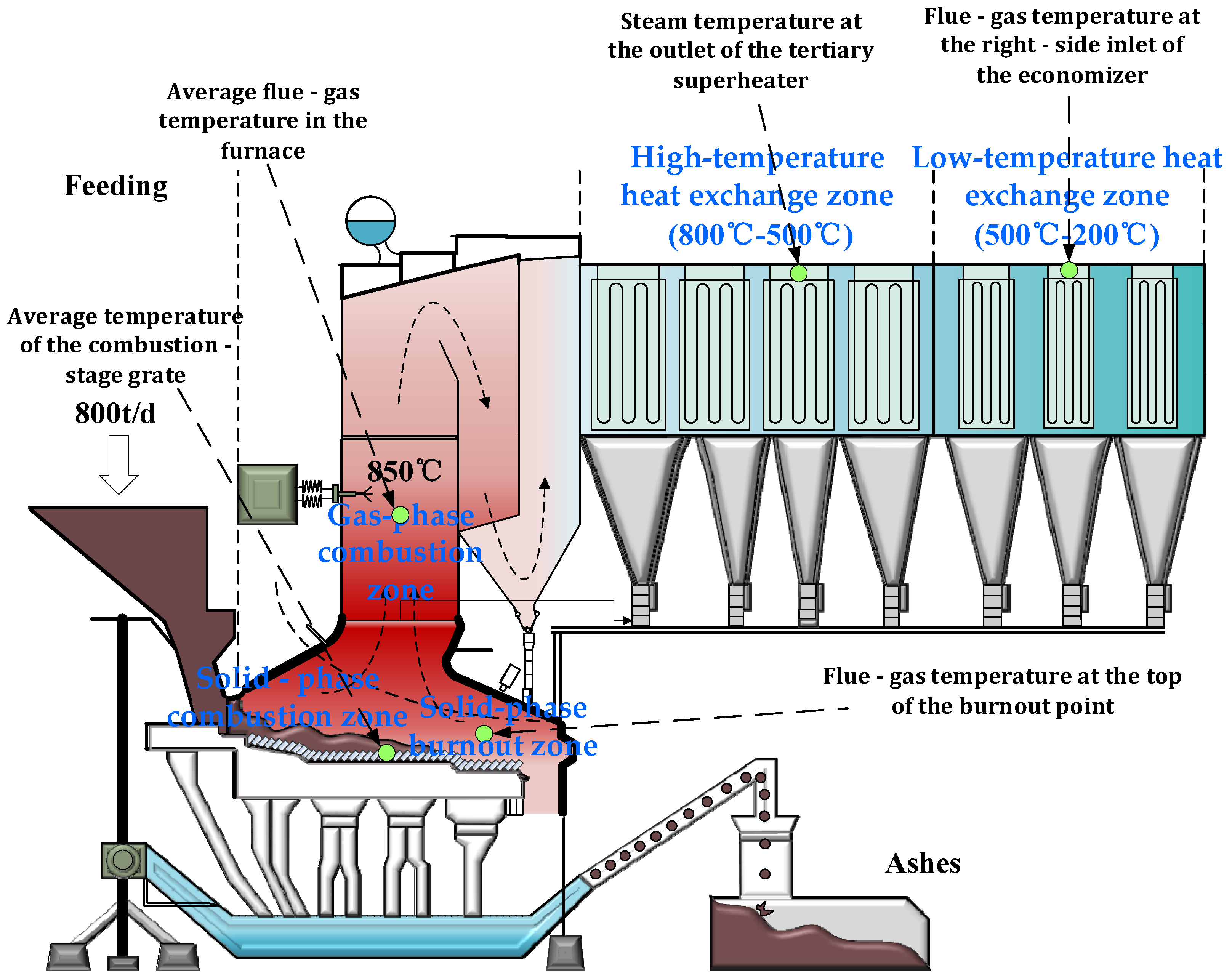
Figure 1. Process flow for MSWI combustion and heat recovery stage.
Sustainability 17 07336 g001
Figure 2. Structure of edge verification platform of an MSWI power plant.
Sustainability 17 07336 g002
Figure 3. Modeling strategy.
Sustainability 17 07336 g003
Figure 4. Correlation analysis diagram of prediction variables.
Sustainability 17 07336 g004aSustainability 17 07336 g004b
Figure 5. Modeling results of the single-temperature-point model.
Sustainability 17 07336 g005aSustainability 17 07336 g005b
Figure 6. Modeling Results of the multi-temperature-point model.
Sustainability 17 07336 g006aSustainability 17 07336 g006b
Figure 7. Comparison of prediction results for the average grate temperature in the combustion section using different algorithms.
Sustainability 17 07336 g007
Figure 8. Relationship diagram between D best min and the multi-temperature-point model R2.
Sustainability 17 07336 g008aSustainability 17 07336 g008b
Figure 9. Relationship diagram between λ and the multi-temperature-point model R2.
Sustainability 17 07336 g009aSustainability 17 07336 g009b
Table 1. Correlation of average temperature of the combustion-stage grate with input parameters (θ = 0.5).
VariablePCC Value
Outlet air temperature of the primary air heater0.7928
Inlet air temperature of the grate in the combustion section0.6467
Cumulative primary air volume of Furnace No. 2−0.7433
Outlet air pressure of the primary air fan−0.6354
Current of the primary air fan−0.6587
Frequency of the primary air fan−0.6754
Table 2. Correlation of the flue gas temperature at the top of the burnout point with each input variable (θ = 0.5).
VariablePCC Value
Temperature on the left outer side of the furnace wall between the drying section and the combustion section grates−0.6545
Temperature of the cooling air outlet on the left side of the furnace wall−0.5226
Temperature of the cooling air outlet on the left side of the grate−0.6889
Table 3. Correlation of the average flue gas temperature in the furnace with each input variable (θ = 0.4).
VariablePCC Value
Right temperature of the slag outlet0.4340
Secondary air heater outlet air temperature−0.4342
Furnace wall left-side cooling air outlet temperature−0.4472
Table 4. Correlation of outlet steam temperature at third-stage superheater with input parameters (θ = 0.5).
VariablePCC Value
Temperature at the cooling air outlet on the right side of the furnace wall−0.4128
Air temperature at the outlet of the combustion section−0.4145
Main steam flow at the boiler outlet0.6584
Boiler drum pressure0.7696
Table 5. Correlation of inlet flue gas temperature at the right-side economizer with input variables (θ = 0.5).
VariablePCC Value
Flue gas temperature on the right side of the first channel0.5837
Flue gas temperature at the right-side inlet of the protection tube0.8222
Main steam flow at the boiler outlet0.7747
Boiler drum pressure0.7725
Steam pressure at the outlet of the tertiary superheater0.5165
Table 6. Hyperparameter values of the single-temperature-point model.
Average Temperature of the Combustion-Stage GrateFlue Gas Temperature at the Top of the Burnout PointAverage Flue Gas Temperature in the FurnaceSteam Temperature at the Outlet of the Tertiary SuperheaterFlue Gas Temperature at the Right-Side Inlet of the Economizer
Minimum number of samples918183151
Regularization coefficient λ i 0.00020.00160.00130.00420.0019
Threshold0.50.50.40.50.5
Table 7. Statistical results of the single-temperature-point model.
Single-Temperature-Point ModelMSEMAER2
Average temperature of the combustion-stage grate0.02950.07360.9984
Flue gas temperature at the top of the burnout point0.94000.66840.9980
Average flue gas temperature in the furnace0.39500.32680.9989
Steam temperature at the outlet of the tertiary superheater0.02900.12900.9985
Flue gas temperature at the right-side inlet of the economizer0.02150.11730.9979
Average value0.28300.26300.9983
Table 8. Statistical results of the multi-temperature-point model.
Multi-Temperature-Point ModelMSEMAE R 2
Average temperature of the combustion-stage grate0.05030.10660.9973
Flue gas temperature at the top of the burnout point2.41411.04730.9948
Average flue gas temperature in the furnace20.58372.51340.9414
Steam temperature at the outlet of the tertiary superheater0.02780.13170.9985
Flue gas temperature at the right-side inlet of the economizer0.02380.12230.9976
Average value4.61990.78430.9859
Table 9. Performance comparison of different algorithms for predicting the average grate temperature in the combustion section.
AlgorithmDatasetMSEMAER2
MeanBestMeanMeanBestMean
RFTraining set0.40390.29440.46470.39420.97810.9840
Validation set0.58350.42820.56580.48120.96840.9768
Testing set0.52830.38600.53660.46180.97130.9791
CARTTraining set0.41980.23590.48430.36780.97720.9872
Validation set0.49730.27330.52580.39800.97310.9852
Testing set0.49320.28770.52030.40400.97320.9844
BPNNTraining set0.31560.07730.42260.21470.98290.9958
Validation set0.32450.07550.41520.21140.98240.9959
Testing set0.32440.07320.42280.21080.98240.9960
LRDTTraining set0.05010.05010.10220.10220.99730.9973
Validation set0.06040.06040.11440.11440.99670.9967
Testing set0.05030.05030.10660.10660.99730.9973
Table 10. Hyperparameter ranges analyzed for the multi-temperature-point model.
HyperparametersValue Range
D best min [15, 35]
λ best [0.0008, 0.0028]
Disclaimer/Publisher’s Note: The statements, opinions and data contained in all publications are solely those of the individual author(s) and contributor(s) and not of MDPI and/or the editor(s). MDPI and/or the editor(s) disclaim responsibility for any injury to people or property resulting from any ideas, methods, instructions or products referred to in the content.