2.4.1. Calculation of Urban Carbon Emissions
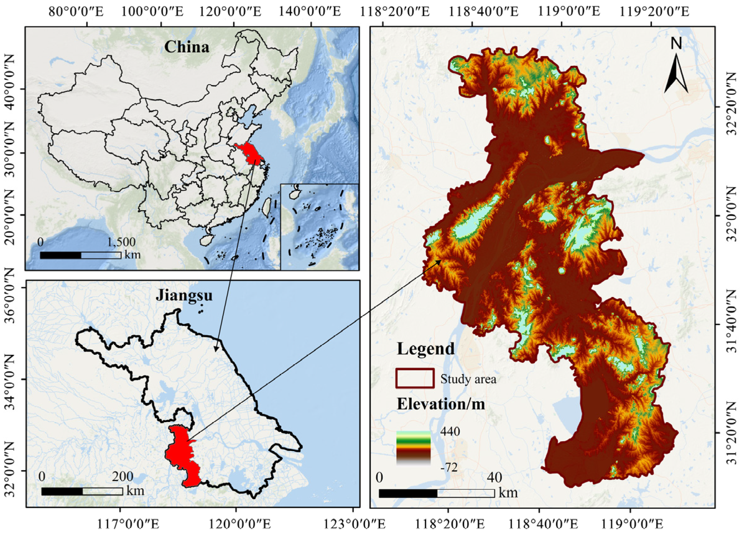
This study uses a multi-scale nested carbon emission accounting system to create a comprehensive carbon measurement framework, with Nanjing as the research object. Municipal carbon emission accounting is based on official statistical data from the China Urban Statistical Yearbook and the China Urban Construction Statistical Yearbook. The measurement method divides carbon emissions into three categories and calculates each separately [
18].
Table 1 outlines the specific classification and calculation methods.
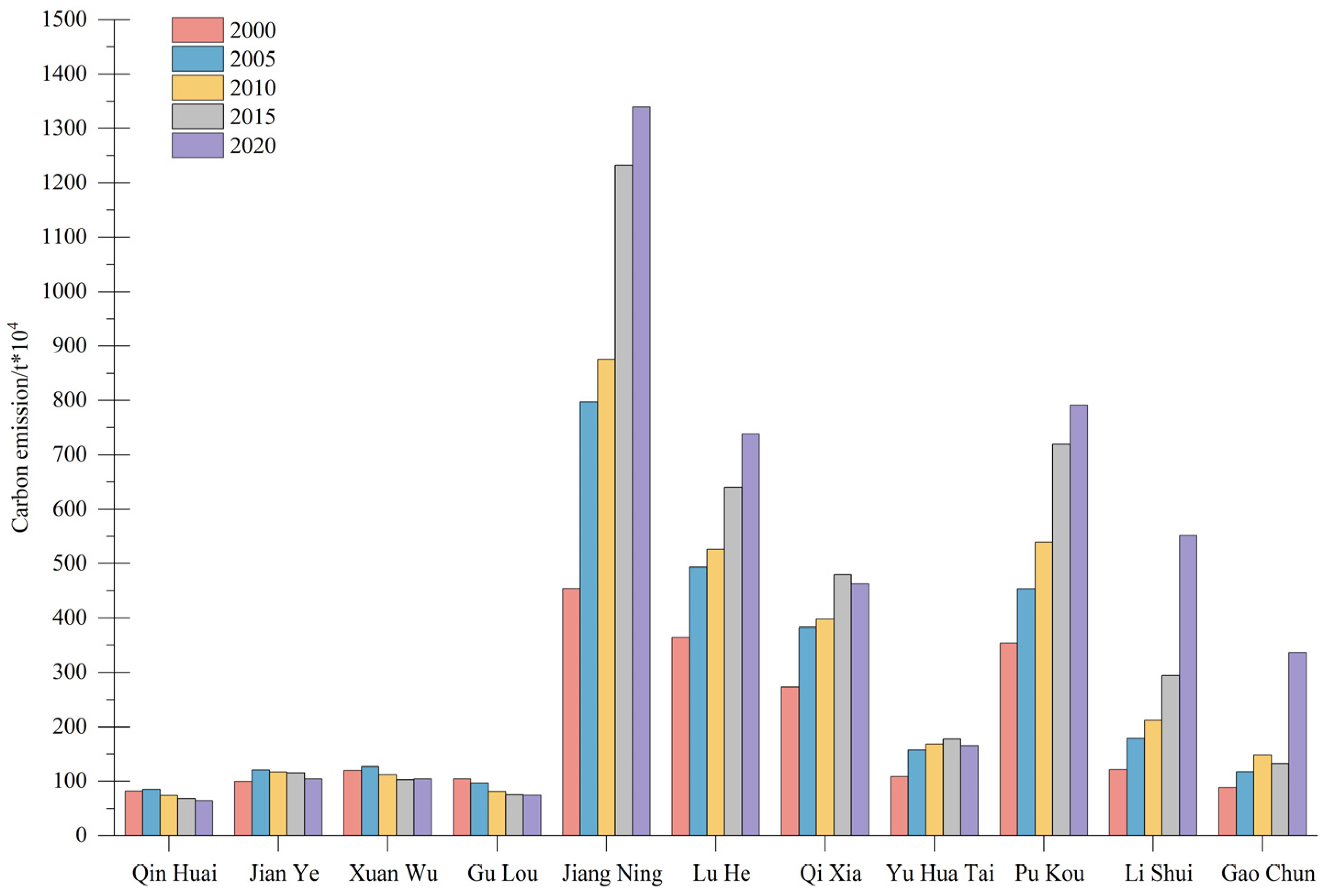
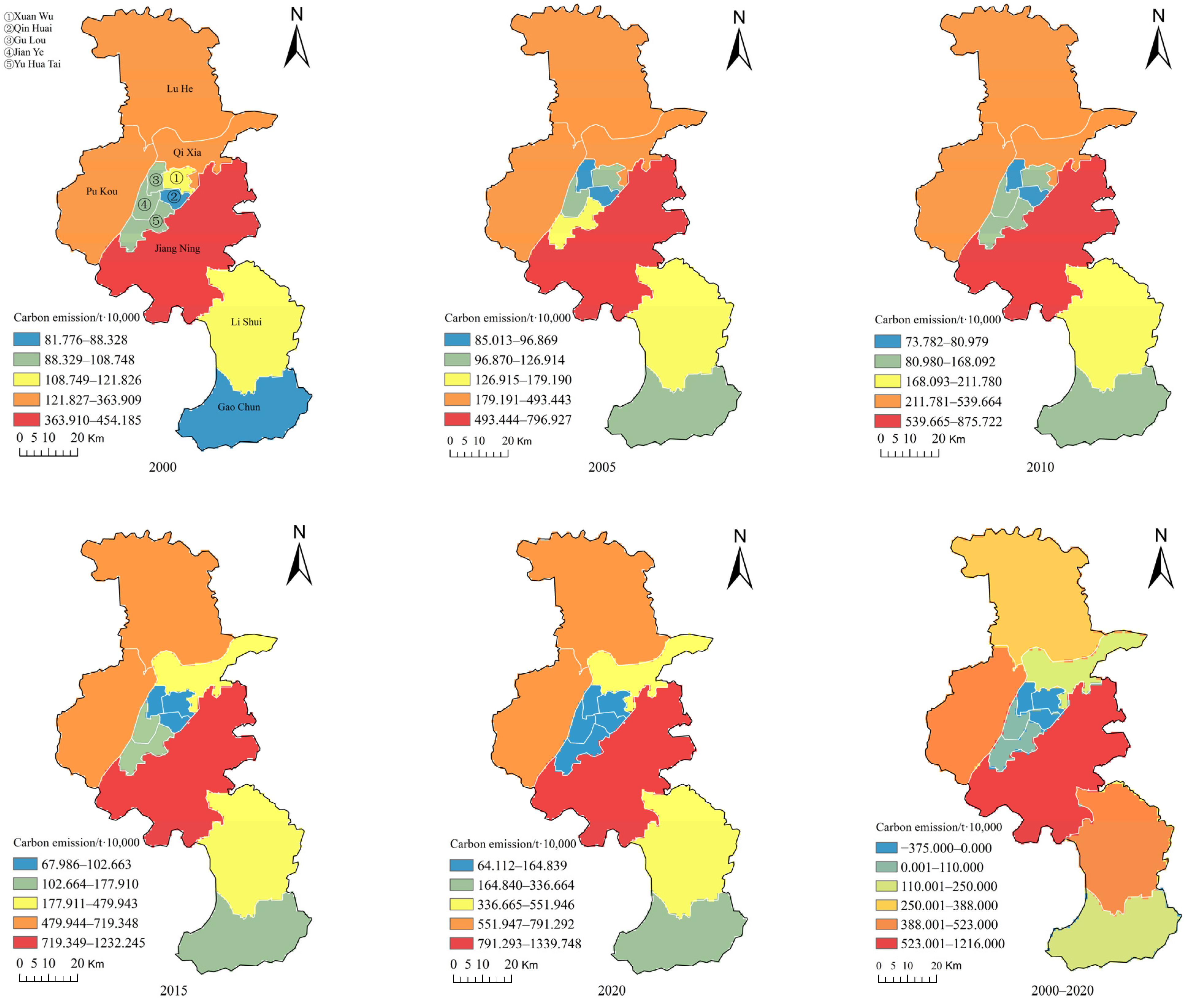
The land use classification method, together with a downscaling model of nighttime lighting data, was used to compute carbon emissions at the district and county levels using municipal accounting. The emission sources were divided into direct emissions (cropland, forest land, grassland, waterways, and unutilized land) and indirect emissions (construction land) [
19,
20,
21,
22,
23]. The following formula was used to determine direct carbon emissions (1). Indirect carbon emissions were defined as energy carbon emissions [
24], and inverse algorithms for district- and county-level carbon emissions were developed using a downscaling model based on nighttime lighting data [
25]. The quantitative association between evening illumination brightness and municipal-level energy carbon emissions in Nanjing from 2000 to 2020 has been calibrated (R
2 > 0.80). The quantitative association between district–county–municipal luminance ratio and energy carbon emissions was estimated using DMSP-OLS nighttime illumination data [
21]. This modeling allowed for the spatial subdivision of energy carbon emissions in Nanjing districts and counties, which were estimated using Equation (2).
In the equation,
is the direct carbon emission (t CO
2e),
is the area of the
ith land use type (hm
2), and
is the carbon emission factor of the
ith land use type (t CO
2e/hm
2) [
26].
In the equation,
is the indirect carbon emissions of districts and counties;
is the municipal energy consumption carbon emissions (t CO
2e);
and
are the nighttime light brightness values of districts and counties and municipalities, respectively; and the discounted standard coal coefficients and carbon emission coefficients of different energy sources in the process of calculating are referred to the research results [
27].
2.4.2. Carbon Emission Estimation Model
The GM (1,1) model is a time series forecasting model based on gray system theory that has a wide range of applications and performs particularly well when dealing with insufficient or complete data. The model’s main idea encompasses a number of critical processes, beginning with the generation of a series by accumulating raw time series data to show the general trend. The cumulative series are then mathematically described by producing a first-order difference equation, also known as a linear first-order differential equation, which displays the data’s pattern of evolution. The next phase in the model’s creation is parameter estimation, which is often accomplished using mathematical approaches such as least squares to get the unknown parameters in the differential equations that correspond to the essential properties of the time series data. Following the completion of the model’s creation, the model test becomes a critical link in ensuring the model’s fitting quality and prediction influence on future data by examining and testing the residuals. The GM (1,1) model is superior due to its simplicity and ease of use, as well as its relatively low computing cost, making it particularly ideal for dealing with easy and irregular time series data, as well as in the context of more scarce or incomplete data. The specific steps and calculation formulas are as follows (
Table 2):
Table 2.
GM (1,1) model step.
Table 2.
GM (1,1) model step.
| Procedure | Formula | Parameter Description | Number |
|---|
| 1. Preprocessing of data | Hypothesized original sequence: | denotes the new sequence obtained by accumulating the original sequence
| / |
| Accumulation sequence: |
| represents the data obtained by accumulating the first k data items of the original sequence | (3) |
| 2. Create a first-order differential equation for | | / | (4) |
| 3. Solve for Equation (3) | | / | (5) |
| 4. Use the least squares method for the values of a and b in Equation (4): | | / | (6) |
|
| 5. Solve for the GM(1,1) model |
| Equation (4) can be solved for the values of a and b to obtain the value of k. Finally, the predicted values can be solved | (7) |
Once the formula is established, the original data series can be fitted and predicted. After the residual model is established, the results need to be taken to the residual test method for diagnostic testing of the model’s effectiveness, based on the original data and calculated data for comparison to calculate the residuals; the use of the mean squared deviation ratio
c and the probability of a small error
P are two indicators of the integrated test to evaluate the accuracy of the indicator prediction model. Let the residuals
at
i moment be
In the above equation,
is the original sequence and
is the sequence obtained after prediction. The subsequent C and P are calculated in the following
Table 3:
Table 3.
Calculation method of mean square difference ratio c and small error probability P.
Table 3.
Calculation method of mean square difference ratio c and small error probability P.
| Procedure | Formula | Number |
|---|
| Mean value of residuals | | (9) |
| Residual variance | | (10) |
| Original sequence mean | | (11) |
| Average relative residuals | | (12) |
| Raw series variance | | (13) |
| Mean square ratio C | | (14) |
| The small error probability P | | (15) |
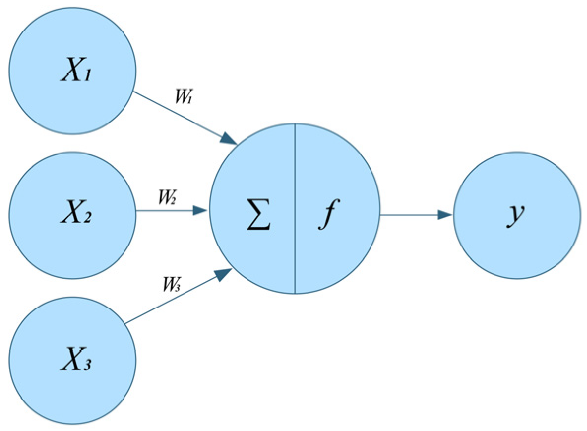
The structure and basic operation concept of neural networks are based on the organization and activity law of the human brain, and they are a simple copy of some of the complex neural network’s particular functions. Neurons are the fundamental building blocks of neural networks, and a large number of synchronized, simple neurons form a complex neural network through signal transmission and processing. A neuron has many basic parallel operation modules, each neuron has an output to which one or more neurons are connected, and each neuron has numerous connection pathways, each of which correlates to a weight, or connection weight. In
Figure 2,
X represents the signal transferred from other neurons, also known as the input signal.
W represents the connection weights between higher-level neurons and lower-level neurons. Typically, there is an additional parameter,
θ. Thus, the relationship between neuron output and input can be stated as follows:
The BP neural network is the most widely used model of neural network; its main operation principle is that for “
n” input learning samples “x
1 x
2 x
3 x
4 x
5⋯x
n”, and its corresponding “
m” output samples are “p
1, p
2, p
3…p
m”. The error between the actual output of the network (z
1 z
2 z
3 z
4 z
5…z
m) and the target vector (p
1, p
2, p
3…p
m) is used to modify its weights, so that the predicted “z” is as close as possible to the desired “t”. Even if the error in the Output Layer of the network is minimized, a BP neural network model with an error within the allowable range of the error can be obtained after repeated corrections of weights. Assuming that the Input Layer of the neural network is x = (x1 x2 x3 x4 x5…xn) T, the number of neurons in the Hidden Layer is is “
h”; then the output value of the Hidden Layer is y = (y
1, y
2, y
3…y
h) T, and the number of neurons in the Output Layer is “
m”; then the output value of the Output Layer is z = (z
1 z
2 z
3 z
4 z
5…z
m) T.
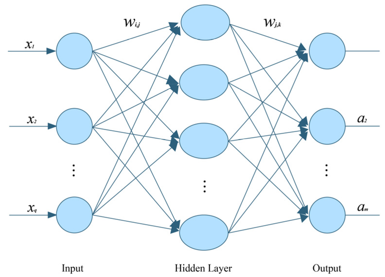
Figure 3 shows the structure of this three-layer typical BP neural network model. In addition, the activation function of Hidden Layer to Input Layer is “
f”, and the activation function of the Output Layer is “
g”. Thus, there is the following:
The output value of the
j-th neuron of the Hidden Layer:
The output value of the
k-th neuron of the Output Layer:
The error between the output value and the target value is
The weight adjustment formula is
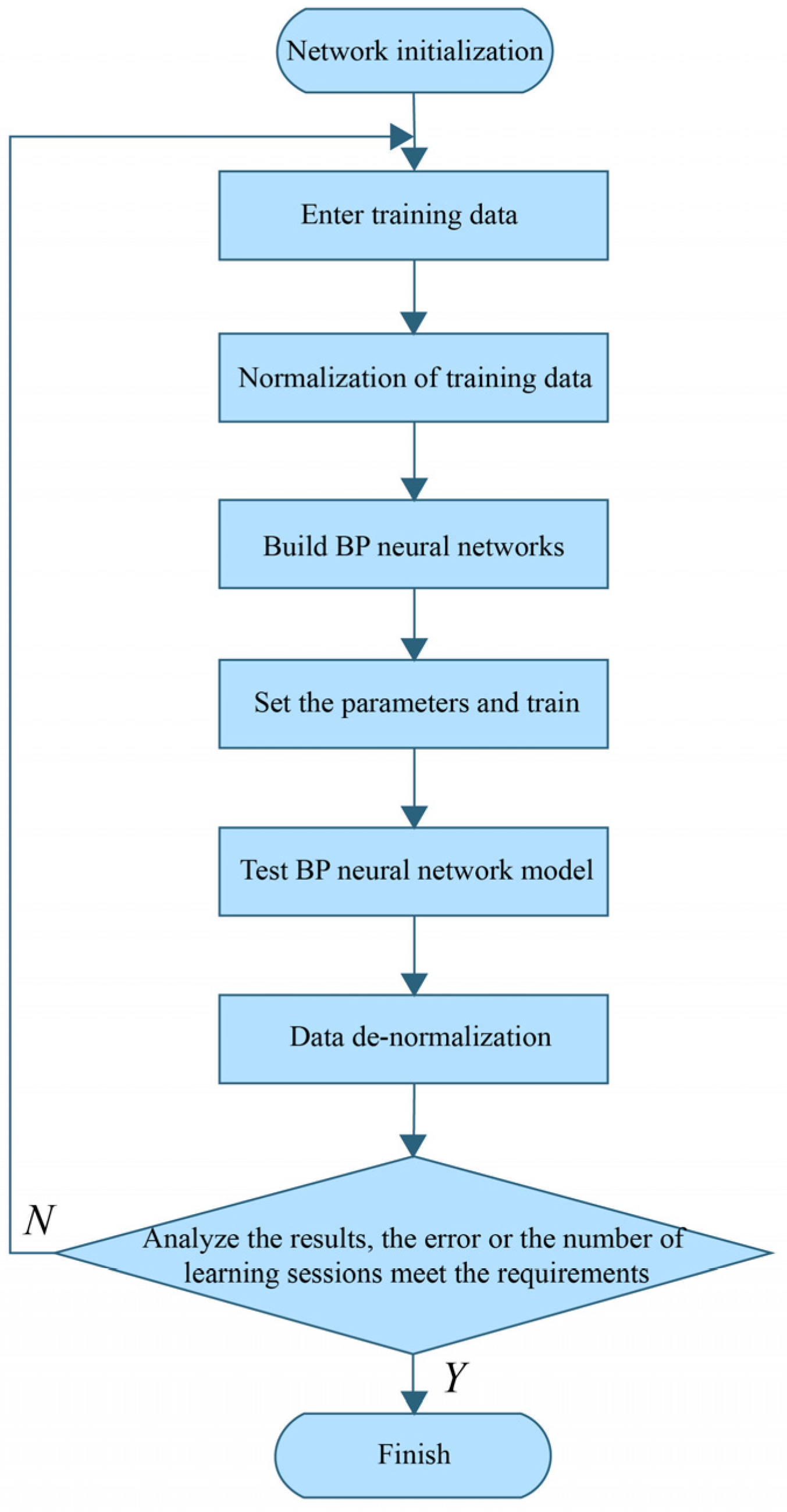
The specific operation flow of the BP neural network is shown in
Figure 4:
The gray BP neural network estimate model is a more advanced and novel engineering cost estimating model that combines the benefits and drawbacks of two algorithmic models: gray theory and the BP neural network. The BP neural network offers significant computer information processing capabilities, including massively parallel, distributed processing, self-organization, self-learning, self-adaptation, prediction, and fault tolerance. With all of these advantages, BP neural networks can improve efficiency and accuracy in prediction applications. Nevertheless, the BP neural network does not include a local self-optimization mechanism in the modeling process. In order to solve some complex nonlinear problems, the BP neural network must constantly adjust and correct the thresholds between the nodes. However, this type of operation is prone to causing the neural network to fall into local minima, which eventually leads to neural network training failure. Furthermore, because the BP neural network algorithm is fundamentally a gradient descent approach, the algorithm process is more complex, resulting in a sawtooth phenomenon, which reduces the BP neural network’s learning efficiency significantly. As a result, the focus of using the BP neural network for modeling is on selecting and processing the beginning values of the training samples to establish the neural network in line with their expected target direction to process and calculate the information data [
28]. The gray system in the modeling process has no hard constraints on the distribution pattern of samples, the quantity of samples, or other information, and the model can be built even with a limited number of data samples. The gray system model also allows for some errors, which can be decreased by modifying the model’s relevant parameters. However, the gray system has flaws as well. This model has few constant parameters, a weak fault tolerance, and quick decreasing and increasing features, making it unsuitable for long-term data analysis and prediction [
29,
30]. Additionally, the gray system lacks the adaptive and self-learning ability of the BP neural network, its information data processing ability is insufficient, and, most importantly, there are serious flaws in error learning during the data and information processing process, which can directly reduce the prediction model’s accuracy.
Based on the above advantages of the gray system and BP neural network and their defects, in the spirit of complementary advantages and disadvantages, the gray system and BP neural network are fused to establish a new algorithmic model; this algorithmic model has been put into automation technology, economic management, the electric power industry, building construction, transportation, and energy use, and other related research and has important uses. The gray BP neural network operates as follows.
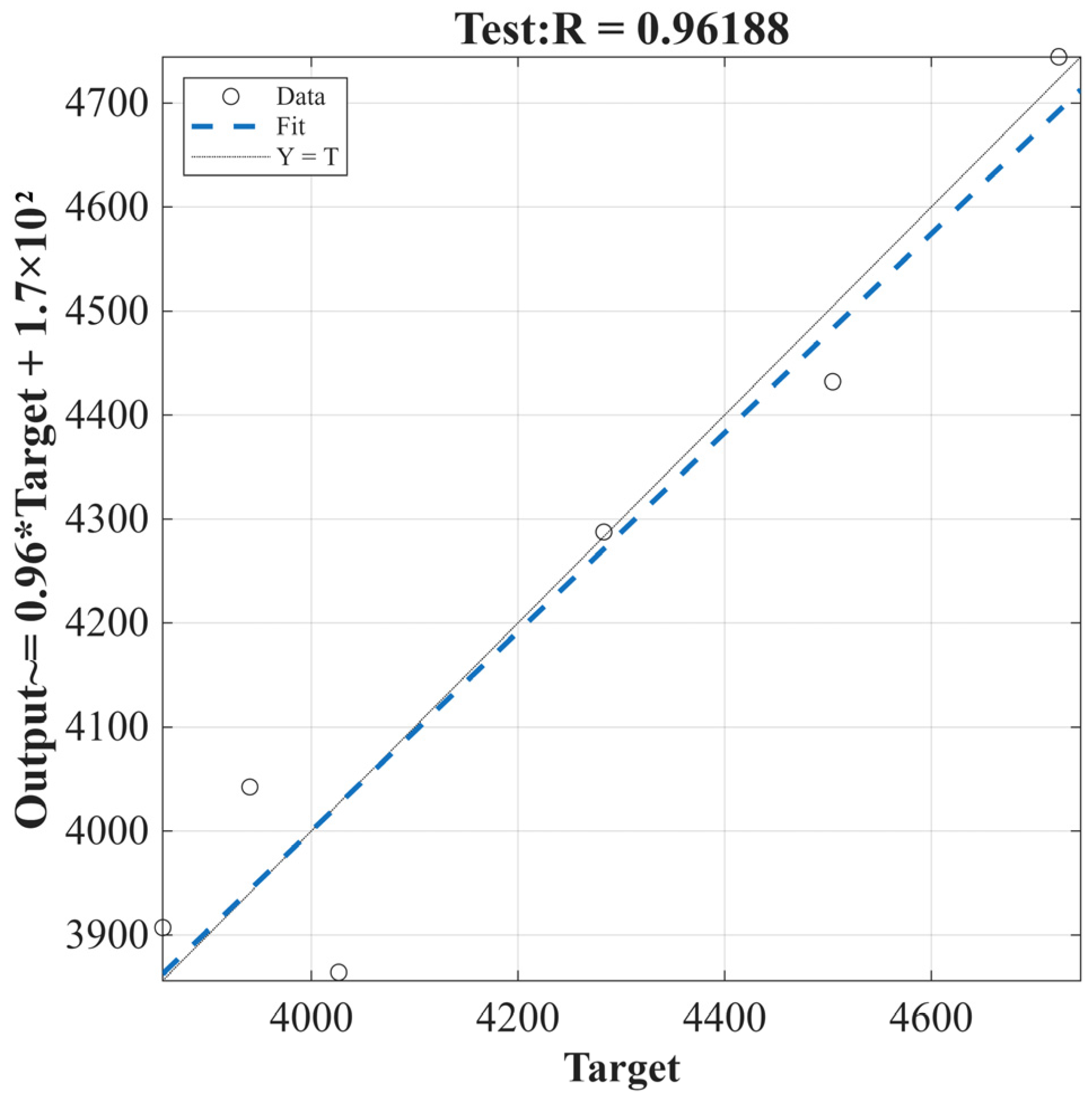
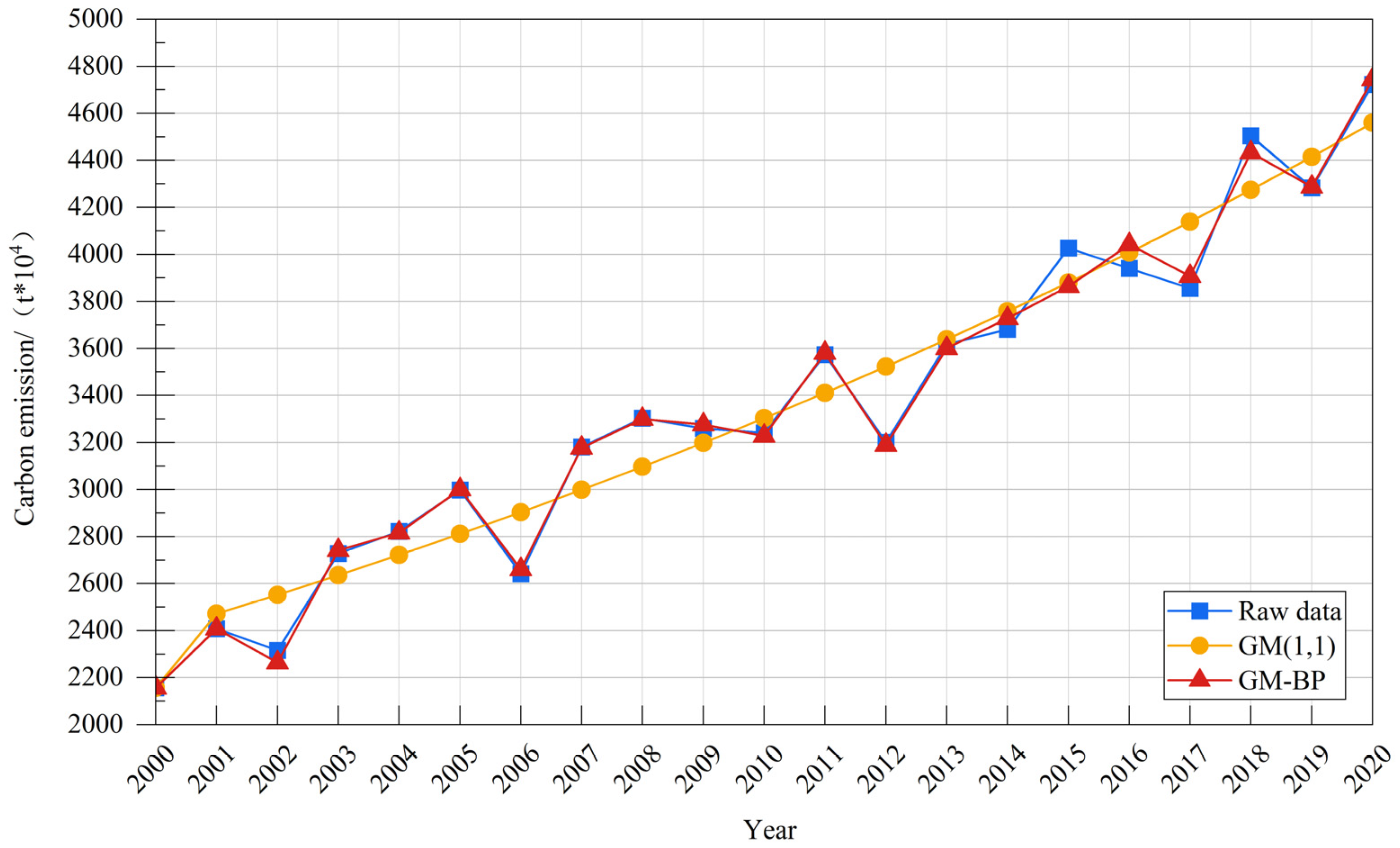
Firstly, the original data sequence is input into the GM (1,1) model to generate the first-order cumulative sequence based on the original sequence, the growth trend of the sequence is reflected through the transformation, and the data sequence generated by the cumulative is modeled by the gray difference and gray differential equations, and the prediction of the cumulative sequence is obtained by solving the parameters using the method of least squares, and finally the simulation and prediction of the original sequence are generated by the cumulative. The number of layers of each neuron are determined, and a BP neural network model is built. Considering that gray simulation values as feature inputs to neural networks can improve prediction stability, both the original data and the data fitted by the gray model are normalized in the neural network. Through forward propagation and error backpropagation in the neural network, the randomly generated initial weights and thresholds are adjusted until the error is less than the preset accuracy, and the prediction results are output. During this process, unspecified hyperparameters (such as the loss function using mean square error (MSE) and the optimizer using gradient descent) follow the standard default configuration of BP neural networks to maintain the model’s simplicity and reduce the risk of overfitting. Combining the outputs of the gray model and neural network, the coefficient of determination (R
2) and mean absolute percentage error (MAPE) metrics are used to verify the prediction performance. For assessing the linear correlation between predicted and actual values, the formula is
where
is the
i-th actual observation,
is the neural network prediction, and
is the average of the actual observations.
2.4.3. Quantitative Characterization of Green Space Morphology
This study quantitatively characterizes the spatial patterns of urban green spaces, with the core objective of revealing how their spatial patterns influence carbon cycling processes within urban ecosystems, ultimately impacting regional carbon emission levels. This analysis is grounded in an interdisciplinary perspective that integrates landscape ecology, ecosystem services, and urban metabolism theory. Based on land use classification standards and the relevant research consensus [
31], this study adopts a citywide coverage approach to define urban green spaces, encompassing all forest and grassland types within the Nanjing municipal area [
9].
The “pattern–process–scale” paradigm [
31,
32] at the core of landscape ecology theory provides key support for this study. This theory emphasizes that landscape spatial patterns profoundly influence ecological flows (such as carbon flows) and ecological processes (such as photosynthetic carbon fixation and respiratory release). Green spaces, as key ecological elements in urban landscapes, have morphological characteristics (such as patch size, shape, connectivity, and aggregation) that directly determine the efficiency of internal ecological processes and the intensity of interactions with the surrounding environment, thereby influencing their carbon sequestration function and ability to regulate external carbon emissions [
5,
33]. For example, large core patches (LPI) may have a higher photosynthetic efficiency and lower edge effects, which are conducive to carbon sequestration, while highly connected (COHESION) green space networks may promote the transmission and integration of ecological flows (including carbon), enhancing the overall resilience and carbon sink capacity of ecosystems [
34].
In addition, the ecosystem services’ theoretical framework clearly defines the important role of urban green spaces in providing key regulatory services [
35,
36]. Green spaces sequester CO
2 from the atmosphere through photosynthesis and indirectly reduce carbon emissions associated with building cooling energy consumption by regulating microclimates (such as mitigating the heat island effect). However, the construction and maintenance of green spaces also involve energy consumption and carbon emissions. Therefore, their net carbon benefits (the net value after carbon sinks offset carbon sources) are key to assessing their impact on regional carbon emissions [
37,
38]. Landscape pattern indices are important tools for quantifying the “potential” and “efficiency” of green spaces in providing carbon regulation services. For example, indicators such as AREA_MN and AI can reflect the scale and spatial organization efficiency of carbon sink core areas, while PLADJ may influence the convenience and energy consumption of maintenance and management.
The theory of urban metabolism views cities as complex systems that continuously input (energy, materials), transform (production, consumption), and output (waste, emissions) [
39]. Within this framework, the urban green space system itself is also a component of urban metabolism. It not only participates in the biogeochemical cycle of carbon (assimilation and absorption), but its spatial characteristics also profoundly influence the carbon emission intensity of other metabolic processes within the city. For example, the distribution pattern of green spaces influences residents’ travel choices (e.g., proximity to parks may encourage walking or cycling, reducing transportation carbon emissions) and the energy consumption of recreational activities; their morphological structure (e.g., large green spaces or ecological corridors) directly impacts the effectiveness of mitigating the urban heat island effect, which in turn affects building energy consumption (particularly cooling); meanwhile their spatial configuration (e.g., highly fragmented or located in high-density built-up areas) is closely related to the material and energy inputs required for their construction and maintenance (implicit carbon emissions) (Dai, 2011; Wang et al., 2021) [
29,
40]. Therefore, analyzing the relationship between green space form indicators (such as TA and PD) and carbon emissions is key to understanding how urban material and energy flows (particularly carbon flows) are spatially regulated by the form of green infrastructure.
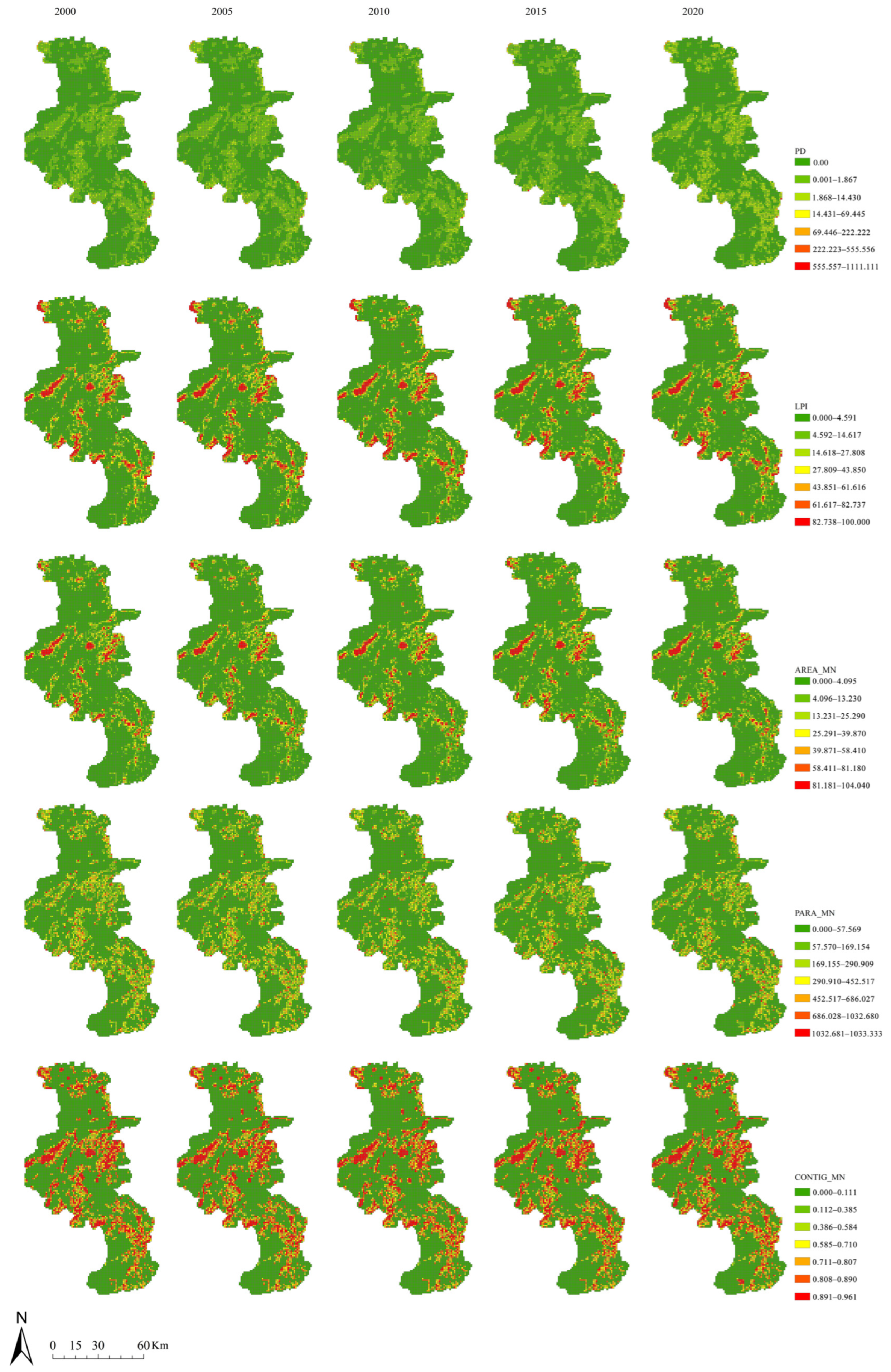
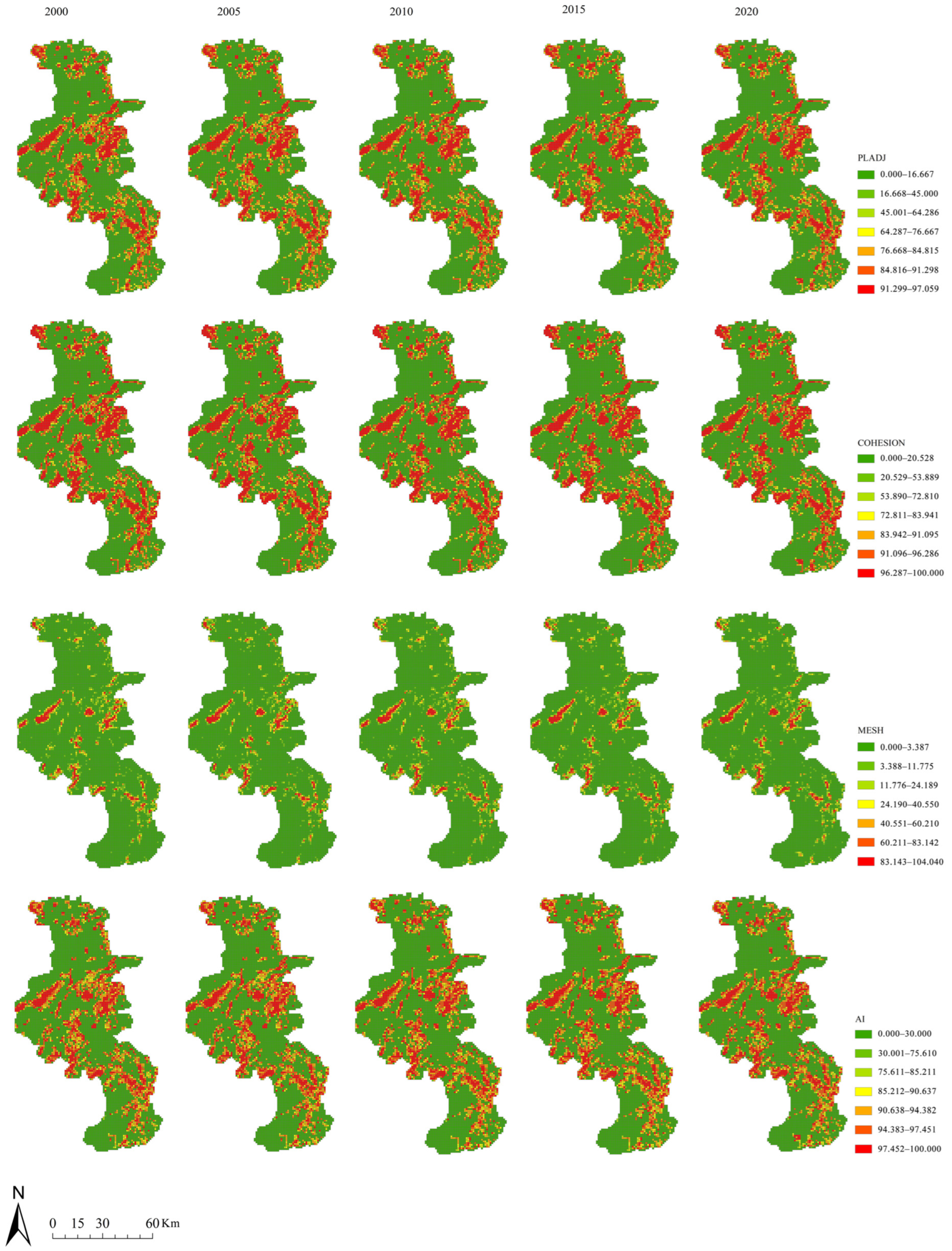
Based on the above theoretical foundations, this study selected 10 landscape pattern indices with clear ecological significance, which respectively assess patch area and shape (e.g., TA, LPI, AREA_MN, PARA_MN, CONTIG_MN), spatial configuration (e.g., PD, PLADJ, COHESION, AI), and overall connectivity (MESH). The specific ecological implications and calculation methods of these indices are detailed in references [
41,
42,
43,
44]. These indices are calculated using FRAGSTATS 4.2 to systematically investigate the following: how green space patterns influence regional carbon emissions by regulating interactions between internal and surrounding environments; which morphological features are more conducive to enhancing the carbon regulation service efficiency of green spaces; and how green space morphology interacts spatially and feeds back with other carbon-emitting processes such as urban energy consumption, transportation, and maintenance management.
