1. Introduction
Global climate change has increased the urgency of reducing carbon emissions, making it a core task for sustainable development around the world. International frameworks, such as the Paris Agreement, have promoted a global consensus on coordinated low-carbon transformation.
As the world’s largest developing country and the largest carbon emitter, China faces enormous pressure. In 2020, China’s greenhouse gas emissions reached the equivalent of 14.6 billion tons of carbon dioxide [
1]. In response, China has put forward the “Double Carbon” goals and incorporated low-carbon development into its national strategy. This is not only a key measure to participate in global climate governance but also a core requirement for achieving high-quality economic development [
2,
3]. In this context, exploring the decoupling relationship between economic development and carbon emissions has become an important issue.
Existing research on carbon–economy decoupling has made progress. Among the various models, the Tapio decoupling model, as a mainstream tool for measuring the coordination between growth and emissions, has revealed significant regional differences. For example, decoupling in Tianjin is more driven by economic growth, while decoupling in Henan is related to the improvement of energy intensity [
4,
5]. However, there are divergent conclusions about the decoupling status between economic development and carbon emissions in Tianjin during the same research period. Some studies believe that it is in a benign decoupling state [
6], while others point out that there is an uncoupling state, which may be related to differences in carbon emission calculation methods [
7]. The uncoupling status in Chongqing and Xinjiang is closely related to their energy structures [
8,
9]. Relevant studies have further confirmed that decoupling is also affected by the industrial structure [
10]. Adjustments to the industrial structure can indirectly affect the decoupling status by changing the interaction between economic development and carbon emissions.
The three northeastern provinces (Liaoning, Jilin, and Heilongjiang) have unique value in exploring the carbon–economy decoupling relationship. As a traditional industrial base, the proportion of industrial carbon emissions in the region has long been above 48% of the total, making it a typical sample for studying industrial emission reduction. There are significant internal differences in the region. Heavy-industrial cities have seen an increase in emission intensity due to the agglomeration of energy-intensive industries, while central cities have shown a decoupling trend through industrial upgrading [
11]. This differentiation provides a rare scenario for analyzing the impact of the industrial structure on the decoupling relationship. At the same time, fluctuations in carbon emissions caused by policies, such as the Northeast Revitalization Strategy, also provide empirical evidence for testing the dynamic impact of policies on the decoupling status [
12,
13].
However, there are obvious deficiencies in the research on the northeastern region. First, most studies focus on the cyclical characteristics of decoupling, ignoring annual dynamic changes, making it difficult to capture the impact of short-term policies. Second, although the industrial structure is considered as a key factor [
14], existing studies only describe its relationship with decoupling qualitatively (for example, pointing out that a high proportion of the secondary industry will hinder strong decoupling [
12,
15]) and have not quantified this relationship.
To fill the above gaps, this study carries out three aspects of work. First, it analyzes the spatial and temporal patterns of carbon emissions and GDP in northeastern cities from 2007 to 2019. Second, it quantifies the decoupling elasticity coefficient through the Tapio decoupling model and the rationalization level of the industrial structure through the Theil index at the municipal scale. Third, it uses multiple linear regression (MLR) to empirically study the relationship between the two. This study hypothesizes that a higher level of rationalization of the industrial structure is more conducive to move toward a strong decoupling state.
This research can provide a basis for formulating policies to balance the relationship between economic development and carbon emissions in old industrial bases and provide reference cases for other similar industrial cities.
2. Materials and Methods
2.1. Research Area
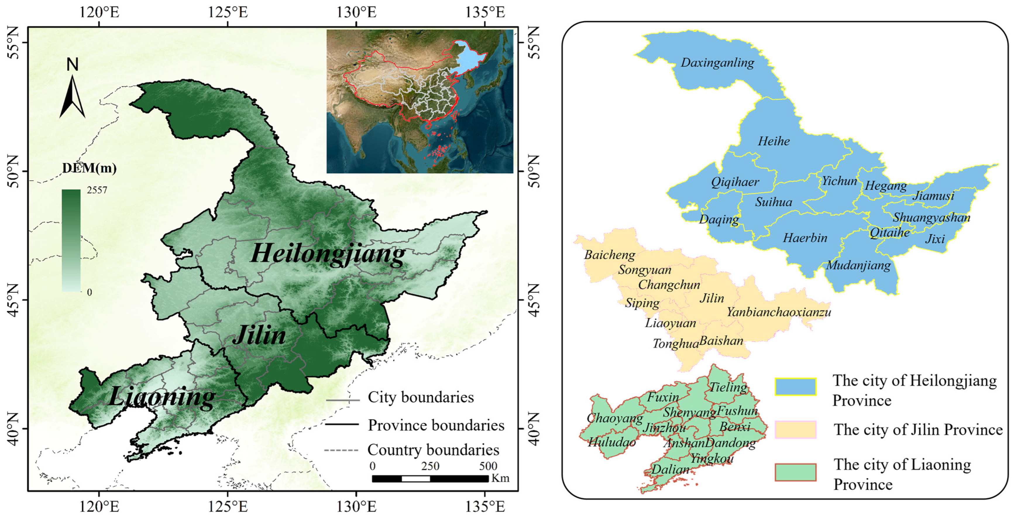
The study area covers the three northeastern provinces of China—Heilongjiang, Jilin, and Liaoning, which are located in the northeastern part of China (
Figure 1). As one of the world’s three major black soil regions, this area accounts for one-fourth of China’s arable land and produces more than 20% of the nation’s grain output. It has long been regarded as the cradle of modern industry in China, with a robust industrial base centered on steel, petrochemicals, and equipment manufacturing, along with several iconic enterprises. The region is rich in energy resources [
16], holding one-third of China’s oil reserves as well as abundant coal and forest resources [
17]. With a population of approximately 100 million and an urbanization rate exceeding 65% [
18], its major cities include Shenyang, Dalian, Changchun, and Harbin. These cities are mainly provincial capitals and megacities and play a significant role in this study.
Since the implementation of the national Northeast Revitalization Strategy in 2003, the economic structure has gradually diversified [
19,
20]. Supported by deepened reforms of state-owned enterprises and the expansion of the private sector, the transformation of traditional heavy industries is accelerated [
21]. However, there are still challenges, including unresolved resource dependence in resource-based cities, increasing population outflow, aging demographics, and lagging low-carbon industrial transformation [
18,
22].
2.2. Data Sources
Carbon emissions from ERGAR are calculated based on the IPCC Guidelines for National Greenhouse Gas Inventories, integrating regional energy consumption data and industry-specific emission factors, while GDP and industrial structure data were sourced from the statistical yearbooks of Jilin, Liaoning, and Heilongjiang Provinces and the
China Statistical Yearbook. The data sources and websites are in
Table 1, and ARCGIS (version 10.2, Esri, Redlands, CA, USA) software was used to conduct visual analysis on the above data.
The study period covers from 2007 to 2019. The selection criteria are as follows: First, the Northeast Revitalization Policy entered a deepening stage in 2007, with the gradual manifestation of policy effects. Second, data from 2020 onward were excluded due to anomalies caused by the COVID-19 pandemic, which led to abnormal economic and social activities, making them unsuitable for a normal reference.
For the two cities with missing data (the Greater Khingan Range region of Heilongjiang Province and Yanbian Korean Autonomous Prefecture of Jilin Province), the data were left blank without any interpolation or imputation methods applied, which resulted in some blank areas in the figures.
2.3. Research Methods
This section will introduce the methods used in this study. First, we use the Tapio model to measure the coordination relationship between carbon emissions and economic development. Second, we calculate the rationalization level of the industrial structure through the Theil index, and based on these two methods, conduct a spatiotemporal heterogeneity analysis on cities in the three northeastern provinces. Finally, we use the multiple linear regression model (MLR) to link the first two through a linear relationship to verify the relationship between them.
2.3.1. Tapio Decoupling Model
The decoupling theory, first proposed by the OECD, aims to analyze the relationships between economic growth, resource use, and environmental pollution. It is widely applied in exploring the link between carbon emissions and economic development, quantifying whether economic growth is decoupled from carbon emissions.
Nowadays, the theory is widely used to study carbon emissions and economic development. In agriculture, scholars use decoupling analysis to explore the dynamic links between greenhouse gas emissions from farming and agricultural growth [
23,
24]. In the energy sector, the theory analyzes the relationship between carbon emissions from energy consumption, industrial growth, and urbanization [
25]. In regional research, decoupling theory evaluates the quality of economic development and informs green policymaking. It provides practical support for global carbon neutrality goals by linking theoretical analysis to sustainable strategies [
26,
27].
The formula for calculating the decoupling state is as follows:
where
D is the elasticity of the decoupling between economic growth and carbon emissions, which quantifies changes in GDP and carbon emissions, and
∆CE and
∆GDP are the value differences between the current and base periods.
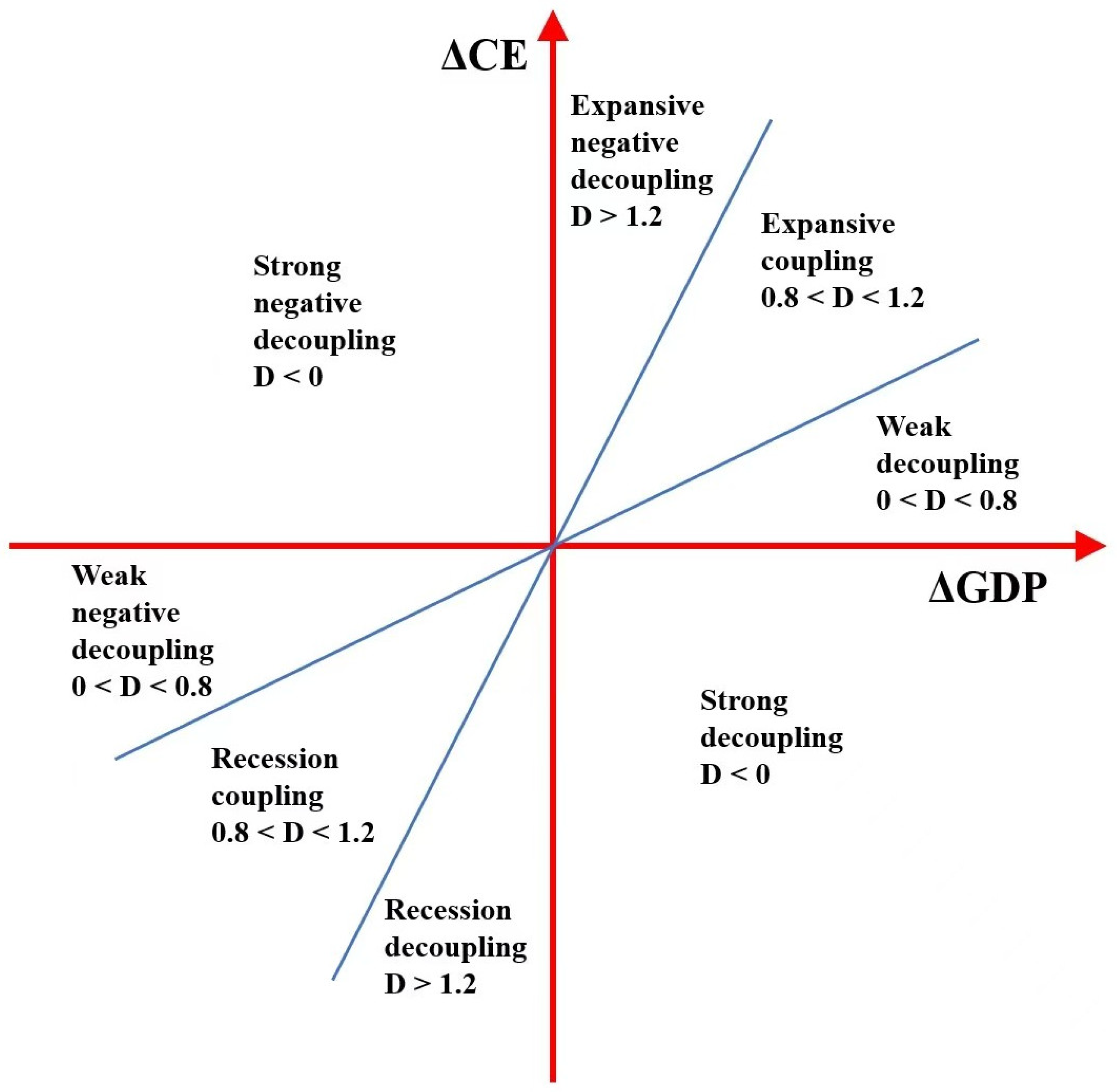
According to Tapio’s classification of decoupling elasticity values, the states can be divided into eight categories: strong decoupling, weak decoupling, expansive coupling, expansive negative decoupling, recession decoupling, recession coupling, weak negative decoupling, and strong negative decoupling (
Figure 2). These states reflect different degrees of correlation between economic growth and carbon emissions. Among them, strong decoupling represents the most ideal state, where carbon emissions decrease while the economy continues to grow. Weak decoupling indicates that the growth rate of the economy is higher than that of carbon emissions, meaning that the separation between the economy and the environment is improving but has not yet reached the ideal state. Expansive coupling means that the growth rates of the economy and carbon emissions are approximately the same. Expansive negative decoupling implies that economic growth is accompanied by a faster growth of carbon emissions, which is a crude and uncoordinated development model. Recession decoupling indicates that the decline rate of the economy is greater than that of carbon emissions, reflecting the deterioration of both economic and environmental conditions, and the economic decline is more severe. Recession coupling means that the decline rates of the economy and carbon emissions are approximately equal. Weak negative decoupling indicates that the decline rate of carbon emissions is relatively low during an economic recession. Strong negative decoupling refers to a situation where carbon emissions increase during an economic recession, posing dual challenges to both the economy and the environment, and represents the worst scenario.
2.3.2. Theil Index
In this study, the Theil index is used to measure the rationalization of the industrial structure. A lower Theil index indicates a more balanced industrial structure and better coordination among industries, while a higher Theil index means a more imbalanced structure. The index takes into account both the proportion of each industrial sector in the overall economy and the differences between industries. The calculation of the Theil index helps to clarify the rationalization level of the industrial structure in the three northeastern provinces, providing a basis for adjusting the industrial structure.
The formula used to calculate the Theil index is as follows:
where
Y represents the total industrial GDP;
Yi (i = 1, 2, 3) correspond to the GDPs of the primary, secondary, and tertiary industries, respectively; and
Yi/Y intuitively represents the output proportion of the ith industry in the total economy, reflecting the industry’s position in the overall economy.
L represents the total number of employed persons in the industry,
Li is the number of employed persons in each industry,
Y/L reflects the total labor productivity of the industry, and
Yi/Li represents the labor productivity of each industry. Additionally,
measures the efficiency difference between industries by comparing the labor productivity of individual industries with the overall average labor productivity.
2.3.3. Multiple Linear Regression Model
A single variable in simple linear regression cannot fully explain the Theil index, as it may be affected by other factors. Thus, a multiple linear regression equation is used to better explain the Theil index. In this study, we performed multiple linear regression equation analysis using IBM SPSS Statistics (
https://www.ibm.com/products/spss-statistics).
The MLR is an extension of the univariate linear regression model, used to simulate the linear relationship between one dependent variable and multiple independent variables. The model can be expressed as follows:
where
y remains the dependent variable;
x1,
x2, …,
xn are multiple independent variables representing different influencing factors;
β0 is the intercept term;
β1,
β2, …,
βn are the regression coefficients corresponding to the independent variables, reflecting the influence degree of each independent variable on the dependent variable; and
µ is the random error term. In the multiple linear regression model, the dependent variable (
y) is the Theil index. Independent variables (
x1,
x2, …,
xn) include the GDP, the elasticity of decoupling between economic growth and carbon emissions, and government spending.
Several tests are conducted to ensure the proper model performance. In this study, we also use SPSS to calculate these tests. The F-test examines whether the model is statistically significant overall and whether all the independent variables jointly affect the dependent variable. The t-test evaluates whether each independent variable has a significant individual effect on the dependent variable. For the p-values obtained from these two tests, we usually compare them with 0.05. If p < 0.05, we consider that there is a significant effect. The measure of the model’s goodness of fit demonstrates how closely the model matches the observed data. The range of R2 is from 0 to 1. The closer it is to 1, the stronger the model’s ability is to explain the dependent variable. The variance inflation factor (VIF) is used to detect multicollinearity among independent variables, since serious multicollinearity can render parameter estimates unreliable. When the VIF is less than 5, we consider the collinearity to be low, and the variables can be used. When the VIF is 5 or greater, we think there is strong collinearity, and variables need to be removed.
3. Results
3.1. Spatiotemporal Heterogeneity Analysis of Carbon Emissions and Economic Development
Spatiotemporal heterogeneity analyses of annual carbon emissions and economic development in the three northeastern provinces from 2007 to 2019 were conducted at both provincial and prefectural city scales. The Greater Khingan Range region and Yanbian Autonomous Prefecture were not analyzed in this study due to missing data, but they will have no impact on the results of this study.
3.1.1. Spatiotemporal Heterogeneity Analysis of Carbon Emissions
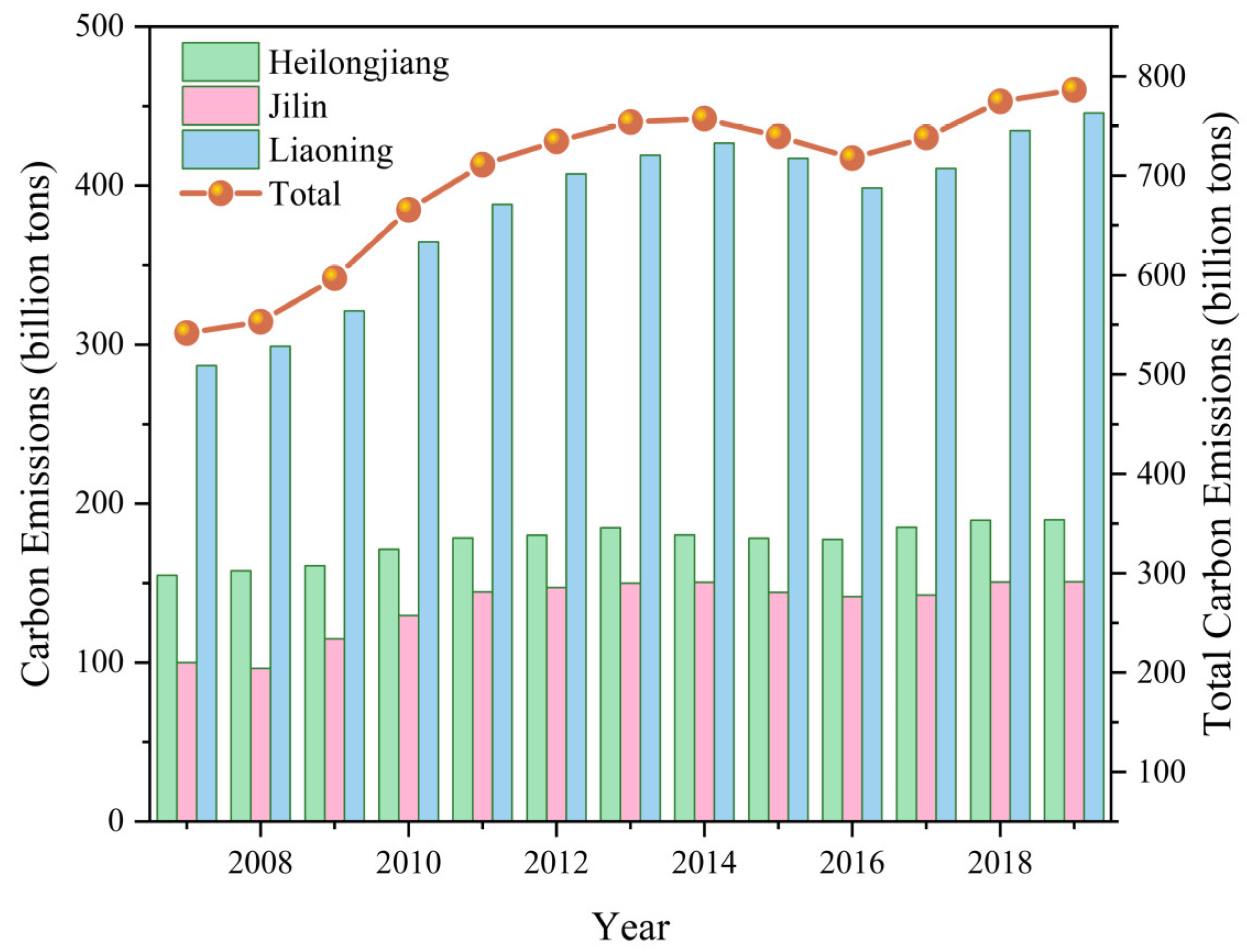
From 2007 to 2019, the total carbon emissions in the three northeastern provinces showed a trend of fluctuating growth, which was divided into three stages. From 2007 to 2014, emissions grew rapidly from 541.70 million tons to 757.59 million tons. From 2014 to 2016, there was a slight decline to 717.61 million tons. From 2016 to 2019, emissions increased again to a peak of 786.45 million tons, and the growth rate in the early period was significantly higher than that in the later period (
Figure 3).
During this period, the carbon emissions of each province in the three northeastern provinces generally increased. The carbon emissions of both Liaoning and Heilongjiang showed an increase–decrease–increase trend, while those of Jilin showed an overall upward trend with fluctuations. The annual average growth rates of the three provinces were Liaoning Province (3.73%) > Jilin Province (3.49%) > and Heilongjiang Province (1.73%). The average carbon emissions of the three provinces were Liaoning Province (386.15 million tons) > Heilongjiang Province (189.87 million tons) > and Jilin Province (135.61 million tons).
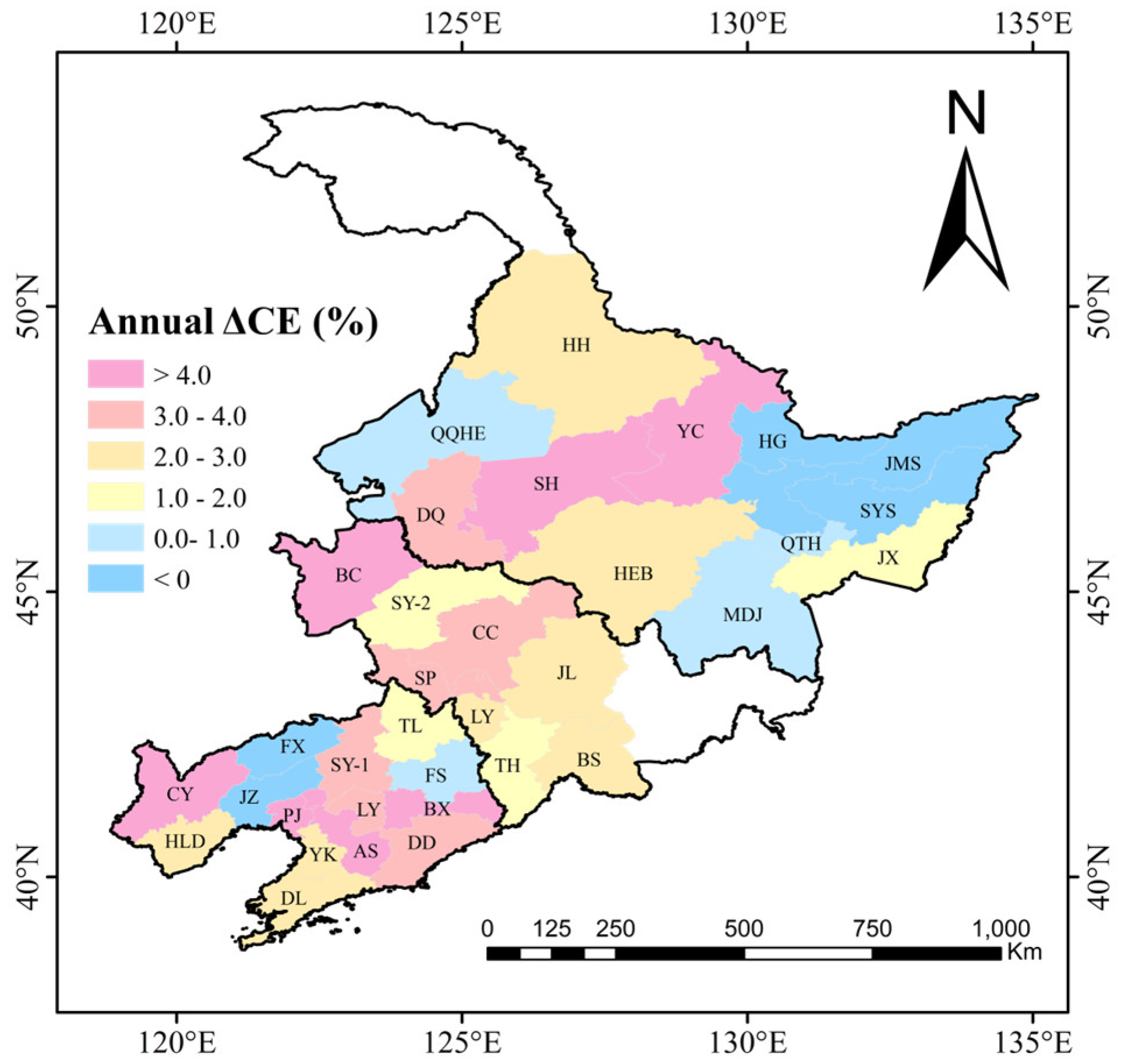
From 2007 to 2019, most prefecture-level cities in the three northeastern provinces showed a carbon emission growth trend with an average growth rate of 2.35% (
Figure 4). The city with the highest carbon emission growth rate was Baicheng (7.34%), and only five prefecture-level cities had negative carbon emission growth, among which Jinzhou had the highest negative growth rate (−2.21%). Adjacent cities had similar growth rates, showing spatial agglomeration.
In Liaoning, from 2007 to 2019, most prefecture-level cities saw carbon emission growth, with an average growth rate of 2.73%. Twelve out of fourteen prefecture-level cities had positive growth, Panjin having the fastest growth at 7.14%. Two cities in northwestern Liaoning showed negative growth, and Jinzhou had the highest negative growth rate at −2.21%. Due to missing data in Yanbian, Jilin analyzed eight prefecture-level cities. All the cities showed carbon emission growth from 2007 to 2019, with an average growth rate of 2.98%. Among them, Baicheng had the highest growth rate at 7.34%, and Tonghua had the lowest at 1.23%. In Heilongjiang Province, due to missing data in Daxing’anling Prefecture, twelve prefecture-level cities were actually analyzed. Most of them exhibited a carbon emission growth trend, with an average growth rate of 1.49%. Nine prefecture-level cities experienced positive growth, and Yichun registered the highest growth rate at 5.85%. Three prefecture-level cities in eastern Heilongjiang reported negative growth, with Shuangyashan showing the highest negative growth rate at −1.93%. The number of cities with negative growth exceeded those in Liaoning and Jilin Provinces.
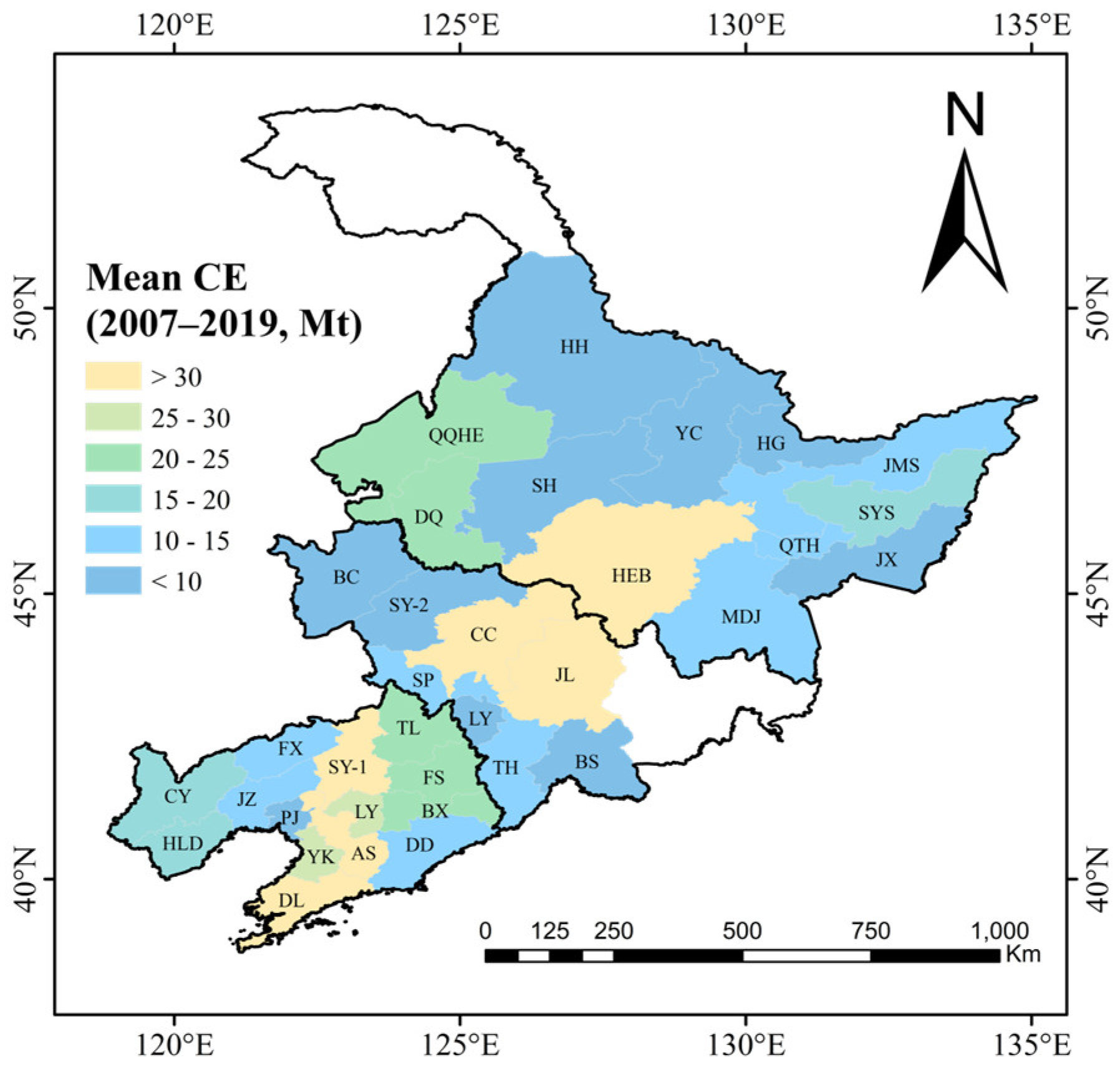
From 2007 to 2019, the average carbon emissions of thirty-four prefecture-level cities in three northeastern provinces were 20.52 million tons. Anshan had the highest emissions at 84.94 million tons, while Hegang had the lowest at 5.35 million tons. High-emission areas were concentrated in the central and southwestern parts of the region, while low-emission areas were distributed in northern, eastern, and central linear zones (
Figure 5).
In Liaoning, 14 prefecture-level cities had an average carbon emission of 27.58 million tons during this period. Anshan ranked first with 84.94 million tons, while Panjin had the lowest at 8.54 million tons. High-emission areas were mainly distributed along the linear region connecting the central cities of Shenyang and Dalian. Low-emission areas were concentrated in the western part of the province. In Jilin, eight prefecture-level cities had an average carbon emission of 16.95 million tons. Changchun had the highest emissions at 40.25 million tons, and Liaoyuan had the lowest at 7.84 million tons. High-emission areas were centered on the central cities of Changchun and Jilin. Except for these two cities, all the other cities had low carbon emissions. In Heilongjiang, 12 prefecture-level cities had an average carbon emission of 14.67 million tons. Harbin led the province with 38.49 million tons, while Hegang had the lowest at 5.35 million tons. Higher-emission areas included the central city of Harbin and eastern Heilongjiang, while low-emission areas were located in the northern and eastern parts of the province.
The results show that regions with high GDPs are mostly central cities and industrial cities, with Liaoning Province being the highest-GDP province. This is closely linked to its high industrial added value and large population [
11,
28].
3.1.2. Spatiotemporal Heterogeneity Analysis of Economic Development
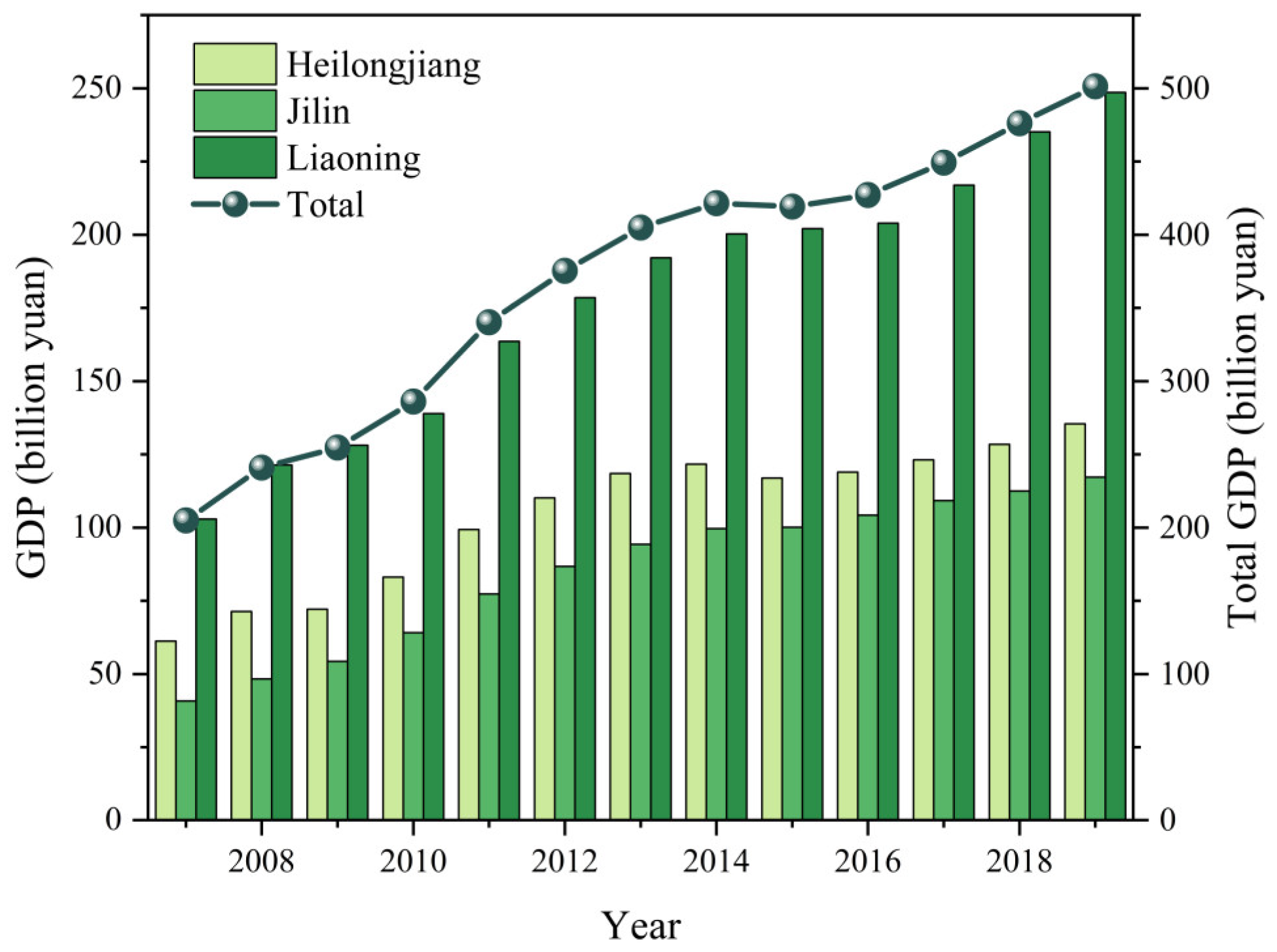
From 2007 to 2019, the total GDP of the three northeastern provinces showed a fluctuating upward trend. It started at 2049.89 billion yuan in 2007, rose to 12,171 billion yuan in 2014, dipped slightly to 11,690 billion yuan in 2015, and, finally, grew to 49,653.5 billion yuan in 2019. The overall trend can be divided into three stages: rapid growth from 2007 to 2014, a minor decline in 2014–2015, and continuous growth from 2015 to 2019. The growth rate in the early stage was higher than that in the later stage (
Figure 6).
During this period, the GDP of each province in the three northeastern provinces grew overall. Liaoning and Jilin both saw steady GDP growth, while Heilongjiang’s GDP showed an upward trend with fluctuations. The average annual growth rates were Jilin Province (9.18%) > Liaoning Province (7.62%) > Heilongjiang Province (6.84%). In terms of the average GDP, the order was Liaoning Province (1794.16 billion yuan) > Heilongjiang Province (1046.52 billion yuan) > Jilin Province (853.19 billion yuan).
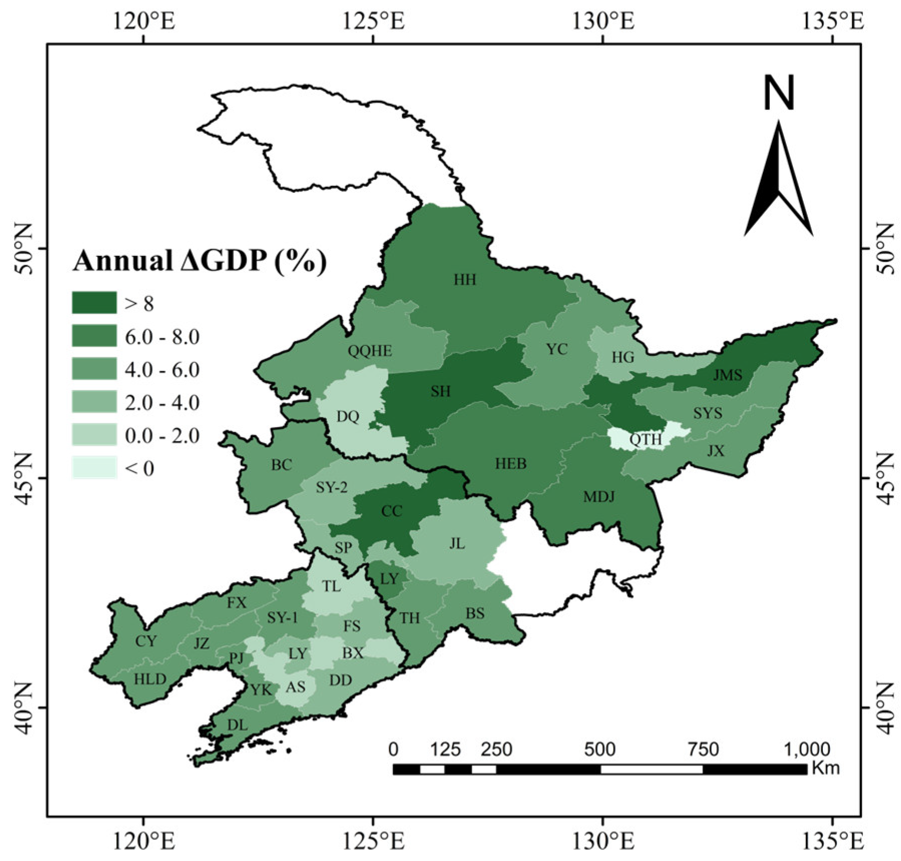
From 2007 to 2019, most prefecture-level cities in the three northeastern provinces grew in GDP (
Figure 7). Among those cities, 33 had a positive growth trend. Changchun had the highest growth rate (8.53%). Only Qitaihe showed negative growth (−1.80%). Adjacent cities had similar growth rates; faster growth was concentrated around Harbin and its surrounding areas.
During this period, all 14 cities in Liaoning experienced positive GDP growth, with an average rate of 3.49%. Dalian had the fastest growth (5.42%), while Anshan had the slowest (0.14%). In Jilin, eight cities were analyzed, and all showed GDP growth. Changchun led with an 8.53% growth rate, while Jilin City (3.34%) and Songyuan (3.33%) had the lowest rates. In Heilongjiang, 12 cities were analyzed, with 11 showing positive growth. Jiamusi had the highest growth rate (8.28%), and only Qitaihe had a decline (−1.80%).
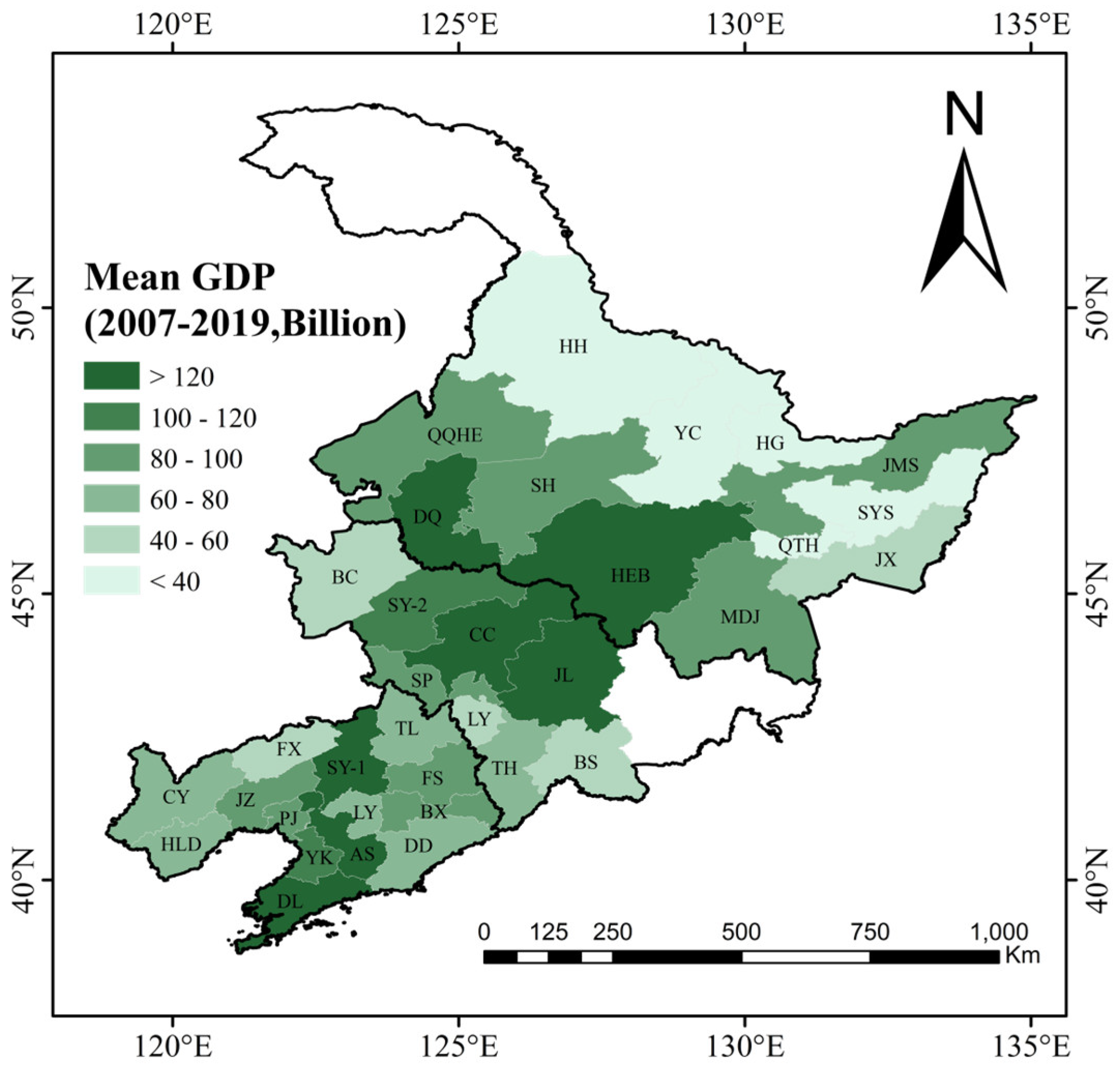
From 2007 to 2019, the average GDP of 34 prefecture-level cities in the three northeastern provinces was 140.67 billion yuan. Dalian had the highest GDP at 624.29 billion yuan, while Yichun had the lowest at 23.60 billion yuan. High-GDP areas were mainly concentrated in central and southwestern linear regions, while low-GDP areas were in northeastern and southern regions (
Figure 8).
In Liaoning, 14 prefecture-level cities had an average GDP of 165.99 billion yuan. Dalian had the highest GDP at 624.29 billion yuan, and Fuxin had the lowest at 43.32 billion yuan. High-GDP areas were concentrated between the central cities of Shenyang and Dalian, while low-GDP areas were in the eastern and western parts of the province. In Jilin, eight prefecture-level cities had an average GDP of 140.52 billion yuan. Changchun had the highest GDP at 467.39 billion yuan, and Liaoyuan had the lowest at 53.25 billion yuan. High-GDP areas were mainly around Changchun and its surrounding cities, while low-GDP areas were in southern Jilin and northwestern Baicheng. In Heilongjiang, 12 prefecture-level cities had an average GDP of 111.23 billion yuan. Harbin had the highest GDP at 468.84 billion yuan, and Yichun the lowest at 23.60 billion yuan. High-GDP areas were mainly in southwestern Heilongjiang, while low-GDP areas were concentrated in the northeastern part of the province.
This result shows that areas with high GDPs are mostly central cities and industrial cities, with Liaoning Province being the highest-GDP province. This is closely related to its high level of industrialization and large population [
29,
30].
3.1.3. Characteristics of Urban Carbon Emissions and GDP
Cities with high carbon-emission levels are mostly industrial cities or central cities. Those with low carbon-emission levels are mostly resource-based cities. Notably, cities with either high or low carbon-emission growth rates are also resource-based cities. Some resource-based cities have reduced carbon emissions through green transformation, while others’ carbon emissions keep rising because their transformation is slow [
31].
Cities with high GDPs and high GDP growth rates are mainly central cities. In contrast, cities with low GDPs and low GDP growth rates are mainly resource-based cities. Some industrial cities also show the feature of low GDP growth rates. While industrial cities and central cities have seen rapid growth in carbon emissions, their GDPs have also been growing. And central cities’ GDPs have grown faster than those of industrial cities. However, resource-based cities have no fixed pattern. This is probably because of differences in policies among these cities [
32].
3.2. Analysis of the Coupling Relationship Between Economic Development and Carbon Emissions, Using the Decoupling Model
To analyze the relationship between carbon emissions and economic development, this study used the Tapio decoupling model to examine the decoupling state. Based on commonly used classification criteria, the eight decoupling states are grouped into three categories: decoupling (strong decoupling, weak decoupling, and recessive decoupling), coupling (expansive coupling and recessive coupling), and negative decoupling (strong negative decoupling, recessive negative decoupling, and expansive negative decoupling). Strong decoupling represents the most ideal state, where carbon emissions decrease while the economy grows. Strong negative decoupling is the worst state, indicating that carbon emissions increase while the economy shrinks. This study calculated the decoupling status of 34 prefecture-level cities in the three northeastern provinces from 2007 to 2019, as shown in
Figure 9.
From 2007 to 2019, the decoupling state between economic development and carbon emissions in Northeast China’s three provinces showed clear periodic and regional differences. From 2007 to 2013, most areas were in strong or weak decoupling states. Only a few eastern regions and areas around Shenyang in the southwest showed coupling or negative decoupling. From 2013 to 2016, negative decoupling concentrated in the northeast. Strong decoupling appeared along a northwest–southeast line centered on Harbin and around Changchun. The southwest saw frequent shifts between negative decoupling and decoupling. From 2016 to 2018, weak decoupling became dominant again, but negative decoupling reappeared in eastern areas and around Shenyang. In 2018–2019, the situation worsened: Only scattered strong decoupling remained in central areas, while most regions experienced negative decoupling.
Liaoning had fewer years of benign decoupling than Heilongjiang and Jilin. Heilongjiang showed mainly strong or weak decoupling from 2007 to 2018, with occasional negative decoupling in eastern and northern areas. After 2018, negative decoupling expanded significantly, leaving only Harbin and a few cities in decoupling states. Jilin experienced benign decoupling in 2007–2013, switched between negative decoupling and decoupling in 2013–2016, and was mostly in weak decoupling in 2016–2018. By 2019, central areas showed negative decoupling, while northwestern areas remained decoupled. Liaoning had weak decoupling in 2007–2013, with negative decoupling concentrated around Shenyang. After 2016, negative decoupling became widespread, though Shenyang still showed some decoupling in 2019.
This result shows that cities with poor decoupling are mainly concentrated in resource-based and industrial cities, which is strongly related to their single industrial structure.
3.3. Analysis of the Industrial Structure Rationalization Using the Thiel Index
Although most regions exhibited a favorable decoupling status, large-scale negative decoupling still occurred in certain years. Due to significant differences in regional industrial structures, this study used the Theil index to measure the rationalization level of the industrial structure and to explore the potential spatial and temporal correlations between the industrial structure rationalization and decoupling status.
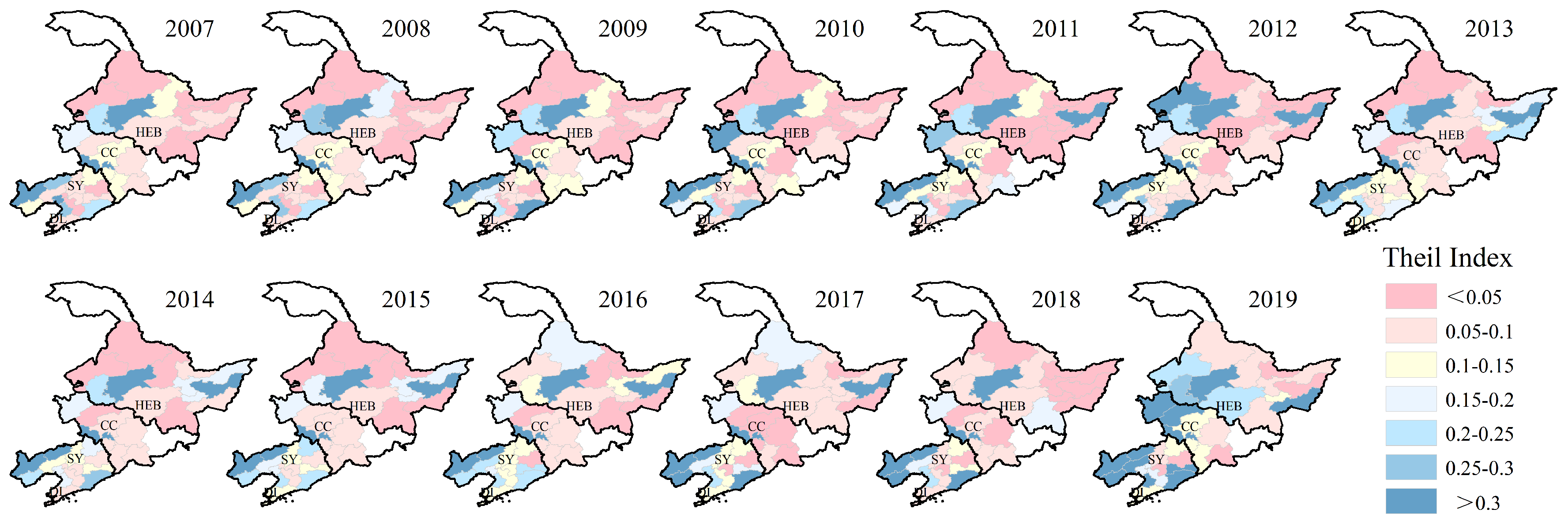
From 2007 to 2019, the industrial structure rationalization index in Northeast China’s three provinces showed clear periodic and regional differences (
Figure 10). High-Theil-index areas (irrational structures) were mainly in the northwestern and southwestern regions, with eastern areas showing high values in 2011–2017 and 2019. Low-value areas were mostly in central and northeastern regions. By 2019, high-value areas in the northwest and southwest had expanded significantly.
For Heilongjiang, high-Theil-index areas concentrated in eastern and western regions from 2007 to 2019, while low-value areas were around Harbin and in northern regions. From 2007 to 2010, the west was the core high-value area; eastern areas joined as a second core in 2011, forming an east–west dual-core pattern. These areas fluctuated from 2012 to 2018, with brief high-value spots in northern regions during 2016–2017. In 2019, the western high-value area expanded to connect to the central region, while a small high-value pocket remained in the east. Jilin had a better industrial structure rationalization than the other provinces. From 2007 to 2018, only one northwestern and one southwestern city had high Theil indexes, while most areas had low values. In 2019, the northwestern high-value area expanded slightly. Liaoning had more high-Theil-index areas, concentrated in the northwestern and southeastern regions from 2007 to 2019. These areas grew in 2017 and 2019. Low-value areas were mainly around the central cities of Shenyang and Dalian.
This result shows that areas with irrational industrial structures are mainly resource-based cities and industrial cities, which are closely related to their single-industrial structure [
33].
3.4. Analysis of the Relationship Between the Thiel Index and the Decoupling Status Using MLR
This study found that both the industrial structure and elasticity coefficient in eastern and southwestern regions exhibited problems, suggesting a possible link between them. To verify this, a multiple linear regression model was constructed. In the model, the elasticity coefficient (D) was set as the independent variable, while the industrial structure rationalization index (Theil index, TL) served as the dependent variable. The model included the GDP growth rate (GDP) and government expenditure (GOV) as control variables to explore the relationship between TL and D. The results of the fitted equation are as follows:
The multiple regression results showed strong overall significance (F-statistic > 10, p < 0.01). The variance inflation factors (VIFs) were all below 5, indicating no serious multicollinearity among the independent variables. The adjusted R2 value exceeded 0.46, showing moderate explanatory power for the dependent variable and a good model fit.
The core explanatory variable, the Theil index (TL), had a significantly positive regression coefficient (β = 0.309, p = 0.02). A higher Theil index was linked to a higher decoupling elasticity coefficient (d). This meant a closer link between economic growth and carbon emissions, including negative decoupling (carbon emissions grow faster than the economy). Conversely, a lower Theil index led to a lower decoupling elasticity coefficient. When GDP grew positively, this tended toward strong decoupling (economic growth with falling carbon emissions).
Among the control variables, government spending (gov) had a significant regression coefficient (t-value < 0.05), showing that local fiscal policies affect decoupling states. However, the GDP had a t-test value of 0.127 (>0.05), failing the significance test. This meant that the economic growth rate alone had no direct impact on the carbon emission decoupling elasticity during the study period.
4. Discussion
4.1. Temporal and Spatial Patterns of Carbon Emissions and Economic Development
Liaoning always had higher carbon emissions and economic development levels than Jilin and Heilongjiang, closely related to its heavy-industry-dominated industrial structure [
34]. The lower carbon emissions in Jilin and Heilongjiang benefited from forest and agricultural carbon sinks [
25] and lower energy consumption [
35].
High-value areas of carbon emissions and economic development were concentrated in central cities, consistent with spatial patterns observed in other regions [
36,
37]. However, a distinct regional feature of Northeast China is that cities with high carbon-emission growth rates were not central cities. It is likely because these non-central cities had smaller initial emission bases and experienced rapid industrial expansion in specific periods [
38], differing from coastal regions, where central cities often drive emission growth through continuous urbanization.
Notably, a few cities in eastern and western Northeast China showed negative carbon emission growth, which seems contradictory to their high-emission industrial structures. This may be attributed to strict environmental policies, leading to reduced production and, thus, lower emissions, and their economic growth is also blocked.
4.2. Decoupling Status and Industrial Structure Rationalization
Tapio model analysis showed that benign decoupling dominated most years from 2007 to 2019, while negative decoupling mainly occurred in 2013–2014, 2015–2016, and 2018–2019, consistent with previous research [
35,
39]. Severe economic downturns from 2013 to 2016 were the main cause of negative decoupling expansion. However, the negative decoupling in 2018–2019 may be also related to the economic downturn caused by population loss and policy lag [
40]. Spatially, negative decoupling is concentrated in the eastern and southwestern regions. Eastern areas were mainly resource-based cities, where declining resource industries caused GDP declines, leading to strong negative decoupling [
33]. Southwestern areas were heavy-industrial cities, where industrial expansion caused carbon emissions to grow faster than the GDP, leading to expansive negative decoupling [
41]. Provincially, prefecture-level cities in Jilin and Heilongjiang had better decoupling states, related to Jilin’s low-carbon agriculture and Heilongjiang’s energy transition [
35,
42]. Liaoning had a worse performance due to its high proportion of heavy industry [
15].
The analysis of the industrial structure rationalization showed irrational industrial structures concentrated in northwestern and southwestern areas, occasionally appearing in eastern areas. Northwestern and southwestern areas were industrial cities, while east-ern areas were resource-based cities, consistent with findings that single-industry structures cause industrial irrationality [
33]. In 2019, the irrational areas showed large-scale expansion, possibly related to industrial hollowing out from overly rapid industrial restructuring [
43]. Jilin had a better industrial structure rationalization through increasing the tertiary-industry share and developing low-carbon agriculture. Heilongjiang had resource-based cities in the east and industrial cities in the west, while Liaoning was mainly industrial cities—both had more high-Theil-index areas, with single-industry structures being the main cause of industrial irrationality.
The study found spatial overlap between the industrial structure rationalization and decoupling status, suggesting an internal connection. However, existing studies lack direct quantitative research on their relationship. They mostly focus on the industrial structure rationalization’s impact on single goals, like emission reduction or economic stability [
44,
45]. This MLR model confirmed a positive correlation between the Theil index and the elasticity coefficient in the decoupling model. This means declining rationalization tends to lead to expansive negative decoupling. This further proved that promoting industrial structure rationalization in Northeast China can improve the decoupling status (toward strong decoupling), and it fulfills the hypothesis proposed at the beginning of this study.
4.3. Policy Recommendations
The results showed that making industrial structures more rational can improve the decoupling between economic development and carbon emissions, but different provinces and regions need different policies [
46].
For resource-based cities in Heilongjiang and industrial cities in Liaoning, with overlapping negative decoupling and high Theil indexes, prioritize industrial restructuring. Heilongjiang should develop biomass energy and an ice–snow economy [
11] to reduce reliance on traditional resources. It can also learn from Shaanxi’s industrial upgrading experience to cut emissions via industrial advancement [
47]. Liaoning needs to accelerate low-carbon tech upgrades in the steel and petrochemical sectors [
48,
49], such as promoting green building materials and carbon capture technologies [
50], following Beijing’s model to shift traditional industries [
51] and referring to Zhengzhou’s experience to drive decoupling through energy efficiency improvements [
52]. While Jilin has fewer negative decoupling and high-Theil-index cases, it also needs to address fluctuations in specific years, such as learning from the Huang–Huai–Hai Plain to boost agricultural efficiency, optimize industrial structures, and expand carbon-sink advantages [
39].
For overall regional development, Northeast China can adopt the Yangtze River Delta model [
39] to establish industrial restructuring mechanisms. This includes orderly transferring high-energy-consuming industries from Liaoning to Heilongjiang and balancing regional decoupling differences through carbon-sink trading. Meanwhile, it can also offer tax incentives to cities with rational industrial structures and strengthen carbon emission controls in cities with poor decoupling. These steps can improve the overall decoupling and achieve coordinated green development [
53].
4.4. Limitations and Future Research
This study has some limitations. The data only cover from 2007 to 2019 and do not include the latest changes after 2020, when the “Double Carbon” goals were further advanced, so they may not show how the decoupling relationship in the three northeastern provinces has changed in recent years. The analysis is at the city level, not going down to districts, counties, or specific industries, making it hard to find more detailed differences. It uses multiple linear regression, which mainly shows linear links between variables and cannot fully capture the non-linear relationship between the industrial structure rationalization and decoupling. Also, it focuses too much on the industrial structure rationalization and does not analyze enough how other key variables interact, which may lead to underestimating the combined effect of multiple factors on decoupling.
Future research can be carried out in several ways. Expand the data to include policy impact analysis after the “Double Carbon” goals were implemented, and compare changes in decoupling patterns before and after the policies. Refine the research to the district, county, or industry level, and combine micro-level enterprise data to analyze the micro-mechanisms of the industrial structural adjustment. Use machine-learning methods to identify the weights of key variables affecting decoupling, making up for the limitations of linear models. Incorporate scenario analysis to simulate the decoupling trends of the three northeastern provinces at key nodes in 2030 and 2060, providing a predictive basis for the long-term path to achieve the “Double Carbon” goals. In addition, this study on the three northeastern provinces can serve as a reference case for other similar regions, but specific applications need to be adjusted according to local policy differences. Future research can use more detailed data to explore the internal mechanisms so that regions with similar mechanisms can gain more experience to learn from.
5. Conclusions
This study systematically explores the relationship between economic development and carbon emissions in Northeast China from 2007 to 2019. It focused on how rational industrial structures affect the decoupling between the two. By integrating the Tapio decoupling model, Theil index, and multiple linear regression (MLR) model, we obtained the following key findings:
(1) Carbon emissions and GDP in the three provinces all showed a “rapid growth–slight decline–regrowth” trend, with clear regional differences. High levels were concentrated in central cities. The decoupling status varied a lot over time and space. Most years had good decoupling, but there were periods of negative decoupling, which were mostly concentrated in industrial and resource-based cities;
(2) The rationality of industrial structures differed by region. Areas with high Theil indexes (showing irrationality) were also mainly in industrial and resource-based cities, mostly due to relying on a single industry. The regression model proved that a higher Theil index (more irrational structure) was closely linked to worse decoupling. It is confirmed that making industrial structures more rational in Northeast China can improve decoupling, filling a gap in direct quantitative research;
(3) The study offers targeted policy suggestions. Liaoning should speed up low-carbon upgrades in the steel and petrochemical industries. Resource-based cities in Heilongjiang can develop biomass energy and an ice–snow economy to reduce resource dependence. Jilin needs to strengthen agricultural carbon sinks. Regionally, setting up industrial restructuring mechanisms can promote coordinated green development. Meanwhile, this study also provides some reference for carbon reduction in similar regions. Future research can expand data, dig deeper into county or industry levels, and use non-linear methods to explore complex relationships, supporting long-term low-carbon transition in Northeast China.
