Electric Bus Battery Energy Consumption Estimation and Influencing Features Analysis Using a Two-Layer Stacking Framework with SHAP-Based Interpretation

Abstract

The widespread adoption of electric buses represents a major step forward in sustainable transportation, but also brings new operational challenges, particularly in terms of improving their efficiency and controlling costs. Therefore, battery energy consumption management is a key approach for addressing these issues. Accurate prediction of energy consumption and interpretation of the influencing factors are essential for improving operational efficiency, optimizing energy use, and reducing operating costs. Although existing studies have made progress in battery energy consumption prediction, challenges remain in achieving high-precision modeling and conducting a comprehensive analysis of the influencing features. To address these gaps, this study proposes a two-layer stacking framework for estimating the energy consumption of electric buses. The first layer integrates the strengths of three nonlinear regression models—RF (Random Forest), GBDT (Gradient Boosted Decision Trees), and CatBoost (Categorical Boosting)—to enhance the modeling capacity for complex feature relationships. The second layer employs a Linear Regression model as a meta-learner to aggregate the predictions from the base models and improve the overall predictive performance. The framework is trained on 2023 operational data from two electric bus routes (NO. 355 and NO. W188) in Changsha, China, incorporating battery system parameters, driving characteristics, and environmental variables as independent variables for model training and analysis. Comparative experiments with various ensemble models demonstrate that the proposed stacking framework exhibits superior performance in data fitting. Furthermore, XGBoost (Extreme Gradient Boosting, version 2.1.4) is introduced as a surrogate model to approximate the decision logic of the stacking framework, enabling SHAP (SHapley Additive exPlanations) analysis to quantify the contribution and marginal effects of influencing features. The proposed stacked and surrogate models achieved superior battery energy consumption prediction accuracy (lowest MSE, RMSE, and MAE), significantly outperforming benchmark models on real-world datasets. SHAP analysis quantified the overall contributions of feature categories (battery operation parameters: 56.5%; driving characteristics: 42.3%; environmental data: 1.2%), further revealing the specific contributions and nonlinear influence mechanisms of individual features. These quantitative findings offer specific guidance for optimizing battery system control and driving behavior.

1. Introduction

With the intensification of global climate change, governments in different countries are placing increasing emphasis on carbon emission reduction. The demand for energy conservation and emission reduction in transportation systems has become increasingly urgent [1]. As one of the primary contributors to global energy consumption and carbon emissions, the transportation system plays an important role in environmental sustainability initiatives. To mitigate environmental pressures, many countries have introduced policies to promote green transportation, recognizing it as a key strategy for addressing climate challenges, and as a result, the adoption of electric vehicles (EVs) has emerged as a cornerstone solution [2]. This policy focus has elevated EV development to a national strategic priority, and it is projected that by 2025, EV sales will exceed 20 million units, accounting for over a quarter of global automobile sales [3]. While the widespread adoption of EVs contributes to carbon emission reduction, air quality improvement, and green transformation of the transportation system, several challenges and limitations persist, including battery range constraints and infrastructure integration issues [4]. Consequently, energy consumption management and range prediction have emerged as critical research areas [5]. EV energy efficiency is influenced by multiple complex factors, including vehicle and system operational status [6], driving behavior [7], climatic conditions [8], and road conditions [9]. A key challenge is minimizing energy consumption and improving operational efficiency without compromising vehicle performance. In this regard, accurately predicting battery energy consumption and analyzing its influencing factors is particularly important, as the battery—the core component of EVs, directly determines the vehicle’s range and operational efficiency. Through precise battery energy consumption prediction, energy waste can be reduced and battery utilization improved, and the battery’s lifespan can also be extended, thereby lowering the vehicle’s operational costs. A comprehensive analysis of various factors affecting battery energy consumption, such as driving behavior, climatic conditions, and battery system status, can help operational departments formulate more accurate energy optimization strategies. Furthermore, accurate energy consumption prediction facilitates more precise vehicle range estimation, which helps alleviate drivers’ range anxiety and enhances their driving experience. From an environmental perspective, reducing battery energy consumption can effectively decrease the overall carbon emissions of EVs and promote the development of greener and more efficient EVs. Therefore, battery energy consumption prediction is not only a key factor in enhancing the economic viability and market competitiveness of EVs but also a necessary means of achieving sustainable transportation and environmental protection goals.

In the prediction and estimation of energy consumption in EVs, existing research has primarily employed two methods: vehicle model-based and data-driven methods. The vehicle model-based approach relies on dynamic models, which are mainly categorized into forward and backward models. Forward models predict the vehicle motion state using driving inputs, such as throttle and brake conditions, steering angle, and other control variables. These models are widely used in industrial simulation software and have become the foundation for several commercial simulation models. In contrast, data-driven methods bypass the reliance on vehicle-specific parameters by directly utilizing the real operational data of vehicles and integrating the factors influencing energy consumption into machine learning models to predict battery energy consumption under complex influencing mechanisms. These methods leverage the powerful data-fitting capabilities of machine learning models, enabling them to handle more complex system features without requiring detailed vehicle parameters, and have gained significant attention in recent years. Although both methods have been applied in their respective fields, several key issues remain unresolved. (1) Vehicle model-based methods offer strong interpretability and can determine the contribution of various factors to energy consumption; however, some vehicle parameters are restricted by manufacturers’ confidentiality agreements, severely limiting the modeling of certain vehicle types. Additionally, when employing vehicle model-based methods for modeling, researchers are often only able to model a specific vehicle model [10,11], hindering broader applications across different vehicle types. Furthermore, some researchers have used auxiliary power models based on specific environmental temperatures and test vehicles that have undergone thermal preprocessing [12]. This implies that the validity of these models may be limited by environmental temperature and the type of test vehicle, rendering them unsuitable for widespread application across all EV types and environmental conditions. (2) Data-driven methods, which construct feature engineering based on real vehicle operation data, have been widely used by many researchers to predict the energy consumption of EVs [13,14,15]. While this approach has strong data-fitting capabilities, the “black box” nature of machine learning models leads to a lack of interpretability, which limits their transparency and reliability in practical applications. Therefore, balancing the predictive power and interpretability of the model remains a critical challenge in energy consumption prediction and estimation. (3) Currently, only a limited number of studies have focused on the impact of battery operating parameters on battery energy consumption [6], which hinders a comprehensive understanding of how the internal operating states of battery systems affect energy usage. Existing research has indicated that power management is closely related to the performance of EVs [16], and some studies have shown that monitoring battery parameters, such as controlling the temperature, is critical for achieving optimal battery operation [17,18]. Against this background, exploring the relationship between battery operating parameters and energy consumption is particularly important, as it may provide a systematic theoretical foundation for improving the energy efficiency of electric buses.

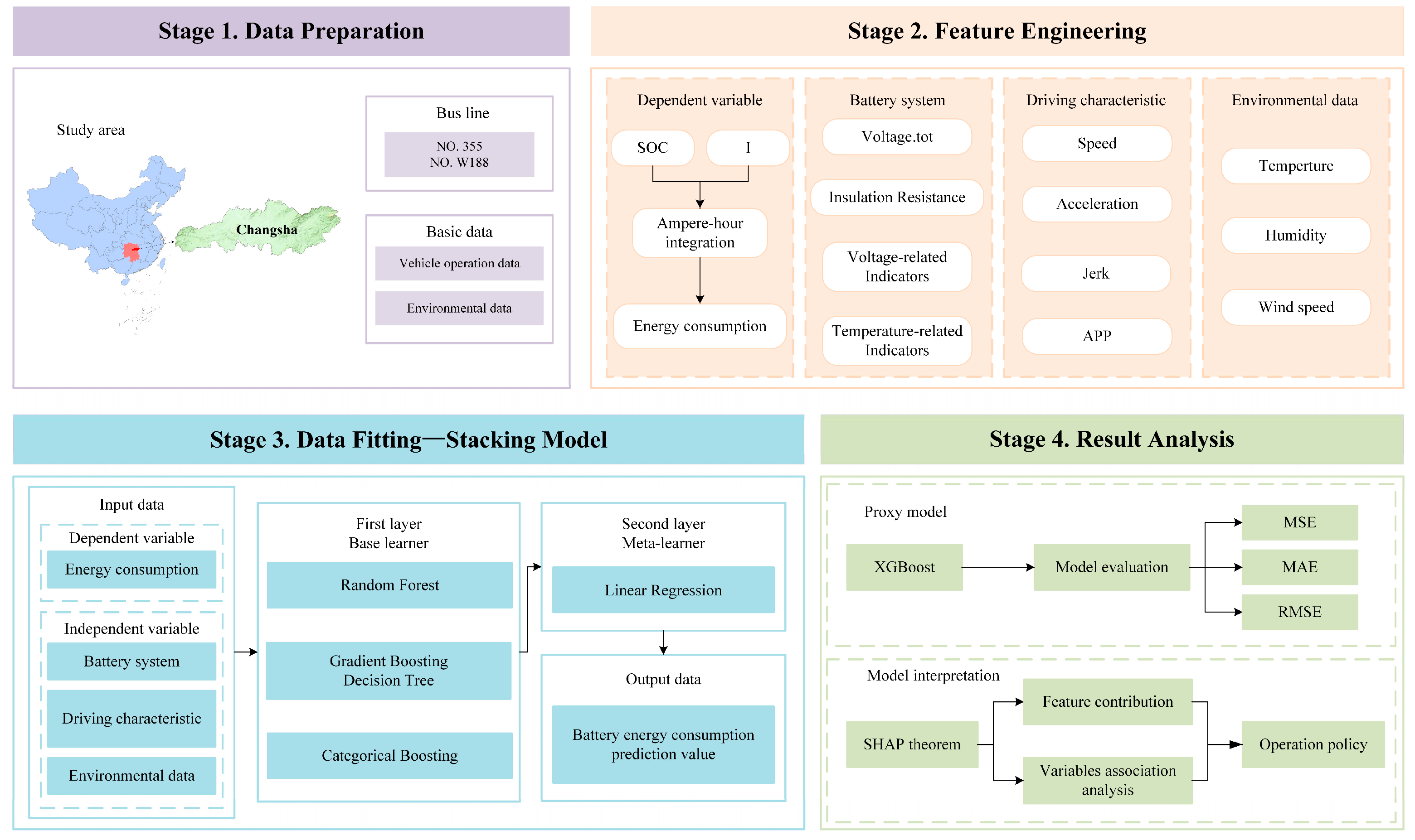
To address the above research gaps and challenges, this study proposes a framework that integrates stacking models, surrogate models, and SHAP analysis to predict the operational energy consumption of EVs and conduct an interpretability analysis. The main contributions of this study are as follows:

(1)

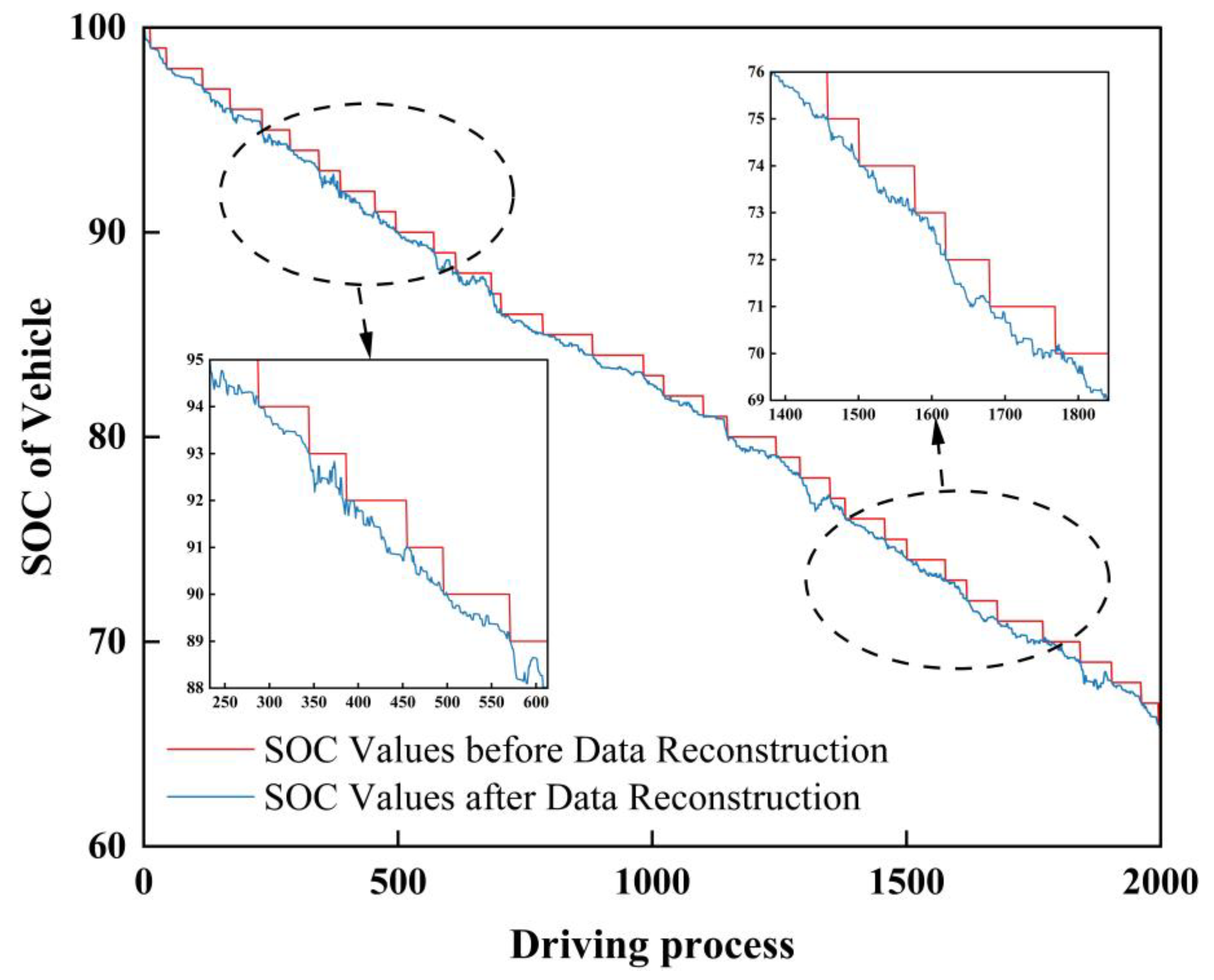
The ampere-hour integration method was introduced to reconstruct the SOC precision and improve the accuracy of the energy consumption computation [19].

(2)

Battery operating parameters were incorporated into the feature set, together with driving characteristics and environmental factors, to construct a more comprehensive system of influencing factors for energy consumption, thereby providing a broader perspective for the subsequent analysis of energy consumption determinants.

(3)

At the modeling level, a unified framework integrating a two-layer stacking model, surrogate model, and SHAP analysis is proposed to achieve a balance between the high-accuracy prediction of EV energy consumption and interpretability of its underlying mechanisms.

(4)

A nonlinear interpretability strategy was developed using the SHAP model to analyze how changes in key indicators affect battery energy consumption, providing deeper insights for formulating more precise energy control strategies and policies.

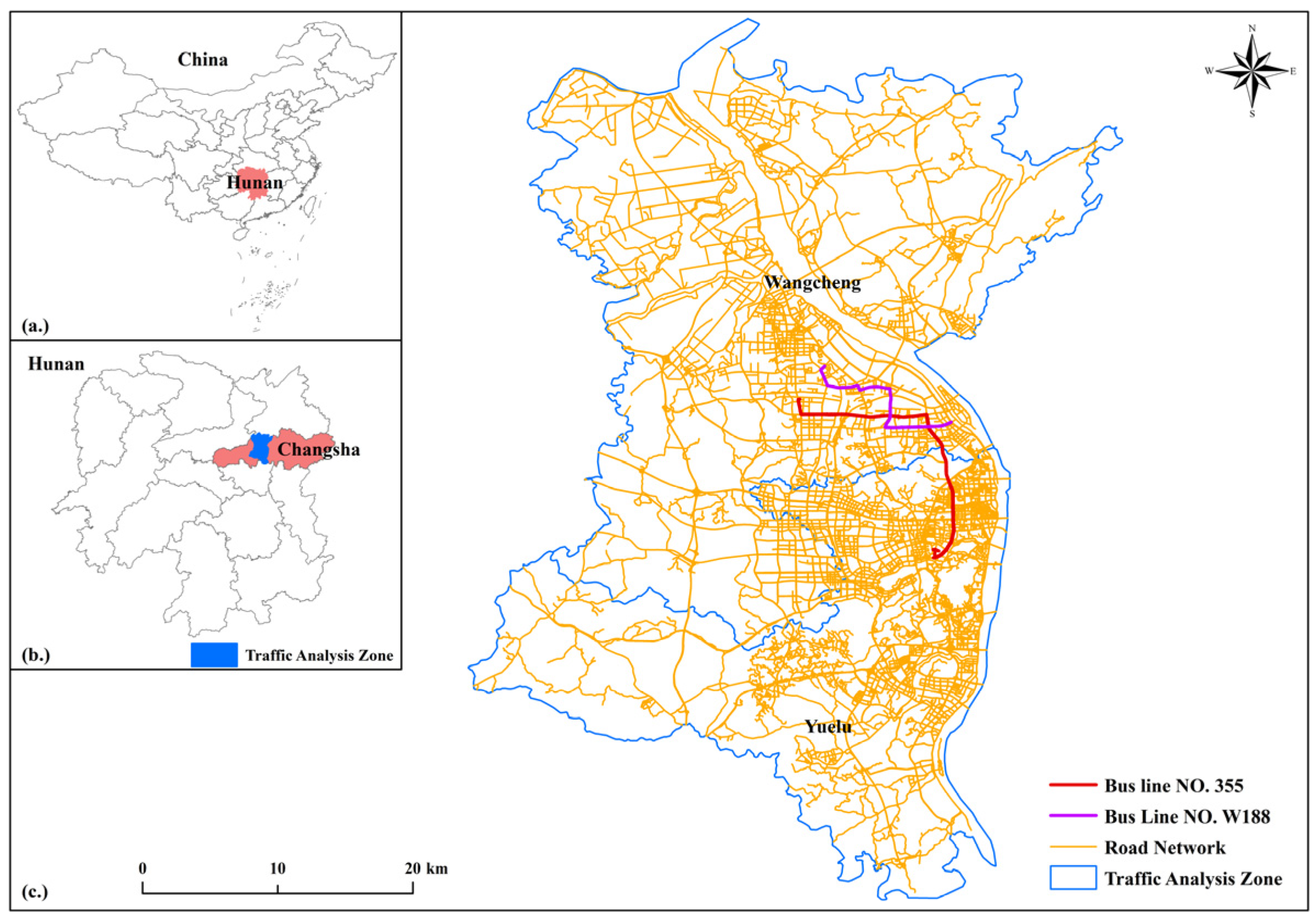
The remainder of this paper is organized as follows. Section 2 reviews the key factors influencing battery energy consumption and examines the methodologies employed in previous studies. Section 3 describes the construction of the indicator system for battery energy consumption, including an overview of the study area and data sources. Section 4 elaborates on the research methodology, detailing the process of fitting and interpreting the battery energy consumption impact mechanisms using the stacking model—surrogate model—SHAP framework. Section 5 presents the model fitting results and an exploratory analysis of the factors influencing battery energy consumption. Section 6 summarizes the key conclusions of this research.

2. Literature Review

In recent years, there has been a significant increase in research on battery energy consumption prediction and analysis of the influencing factors for EVs. Scholars generally select influencing factors from aspects such as battery system parameters, driving characteristics, environmental conditions and route characteristics. Additionally, methods for predicting the energy consumption of EVs are generally classified into two primary categories: vehicle model-based methods and data-driven methods. Both approaches have been extensively studied and applied in recent research.

2.1. The Influencing Factors of Battery Energy Consumption

This section summarizes the factors selected for EV battery energy consumption prediction from four categories: driving characteristics, environmental conditions, route characteristics, and battery system parameters.

Driving characteristics have been widely recognized as significant factors influencing the energy consumption of new energy batteries and have been extensively applied in energy consumption prediction research. Under identical road, environmental, and vehicle conditions, variations in driving habits and behaviors can lead to differences in energy consumption values. Zhang et al. demonstrated in their analysis and prediction of EV energy consumption that battery energy consumption is highly correlated with driver behavior characteristics, particularly the speed and acceleration [20]. He et al. analyzed the relationship between energy consumption reduction and acceleration time and found that controlling driving behavior, such as extending the acceleration time, is key to reducing energy consumption during acceleration, emphasizing the significant impact of driving behavior on EV energy consumption [21]. Zhang et al. conducted an energy consumption characteristic analysis based on microscopic driving parameters and found that the energy consumption rate of EVs increases with higher instantaneous speed and acceleration [4]. The driving characteristics reflected by the use of the accelerator and brake pedals also impact energy consumption. Moreover, during acceleration, the proportion of energy consumption exceeds that of deceleration because kinetic energy can be recovered and converted into electrical energy during coasting or braking [22]. Lárusdóttir et al. conducted a comprehensive study on the energy consumption of various vehicle types, analyzing the impact of driving behavior and vehicle characteristics [23]. They concluded that extreme acceleration behaviors significantly increase energy consumption, whereas moderate acceleration and stable driving speeds contribute to energy conservation [23]. In addition to the aforementioned indicators, Huang et al. introduced the degree of accelerator pedal depression in an energy consumption prediction model based on driving behavior to intuitively assess driving characteristics, achieving an accuracy of 98%. Simulation results showed that differences in the degree and frequency of accelerator pedal depression among drivers significantly impacted battery energy consumption [24].

Environmental factors are less frequently incorporated into related studies due to the challenges associated with their observation; however, existing research has demonstrated their significant impact on battery energy consumption. Vepsäläinen et al. introduced environmental factors into the energy consumption prediction of three bus routes in southern Finland using a linear model and achieved a prediction accuracy of 75%. The study found that ambient temperature is the most influential environmental factor contributing to energy consumption uncertainty [8]. In their study on the sensitivity of EV propulsion power to environmental factors, Yi et al. highlighted that environmental variables, such as temperature and wind speed, have a profound impact on the overall energy consumption of EVs and significantly affect the remaining range of the vehicle [25]. In developing an energy consumption model for electric buses and optimizing the charging schedule, Gao et al. incorporated special conditions, such as rainy weather, into the model and considered humidity levels as a critical environmental variable [26]. Ambient temperature has been consistently identified as the primary environmental factor influencing battery energy consumption [27]. However, research on the effects of other environmental variables, such as humidity and air pressure, remains limited.

Building on the above, some studies have classified the factors influencing battery energy consumption into internal and external factors. For external factors, in addition to environmental variables, some studies have incorporated route characteristics into the indicator system, typically measuring these characteristics based on the number of bus stops and traffic lights along a route. For instance, Gallet et al. emphasized the role of bus stops in estimating the energy demand of electric buses [28]. Their longitudinal dynamics model effectively utilizes low-resolution operational data, such as bus arrival and departure times at each bus stop, to accurately calculate energy demand, revealing that the heterogeneity of driving conditions leads to significant variance in energy requirements across different routes and at different times of the day. It also demonstrates the good potential for fast charging during layover times by quantifying the energy demand of bus routes between stops. Similarly, El-Taweel et al. introduced trip length and the distance between consecutive bus stops as key indicators in their energy consumption model while modeling bus routes in regions such as Brampton, Canada. They generated speed profiles to reflect real-world traffic conditions and speed behaviors for energy consumption modeling [9]. Regarding internal factors, existing research primarily focuses on driving characteristics, with some studies incorporating the internal parameters of the vehicle battery system into the indicator framework. For example, Wu et al. considered the voltage, current, and resistance of a battery pack when estimating the instantaneous power and trip energy consumption of EVs [6]. Fotouhi et al. incorporated SOC-related indicators into battery energy consumption estimation [29]. The introduction of these battery system parameters helps shift the analytical perspective of battery energy consumption toward the vehicle’s battery system, offering new insights into battery system design and the development of energy-efficient EV models.

2.2. Predictive Methods

This section reviews the two primary predictive methods for estimating the battery energy consumption in EVs: vehicle model-based and data-driven methods, each with its strengths, limitations, and applications in energy consumption prediction.

Vehicle model-based methods have been widely applied in simulation software. For instance, Cioroianu et al. developed an EV model and simulated the energy consumption of the Dacia Sandero using AVL Cruise software, obtaining an average energy consumption result of 15.19 kWh/100 km [30]. Similarly, the Argonne National Laboratory developed a vehicle simulation tool called Autonomie, which, in simulations of hundreds of thousands of vehicles, demonstrated that the prediction error fell within ±3% of the observed values. This simulation tool has become a standard tool for analyzing vehicle energy consumption [31]. Backward models often utilize Longitudinal Dynamics Models (LDM) and Vehicle Specific Power (VSP) models, both of which have extensive applications [20]. For example, Wu et al. developed an LDM-based model to estimate energy consumption by incorporating the vehicle speed, acceleration, road slope, and other driving parameters. In the energy consumption prediction for over 40 trips, the average MAE for all journeys was 15.6% [6]. Fotouhi et al. integrated a vehicle model, driver model, and terrain model to develop an energy consumption estimator with an estimation error of less than 3% in field tests on specific routes [29]. Zhang and Tian developed a vehicle-driven energy consumption prediction model by analyzing vehicle performance, extracting road features, and calculating wheel forces under varying road conditions. Simulation results showed that after a hybrid vehicle traveled more than 60 km, its power consumption dropped to below 1 kW [32]. Although vehicle model-driven methods are widely applied and offer strong interpretability compared with data-driven models, they require a large number of vehicle-specific parameters during the modeling process, which may be constrained by vehicle type variations and proprietary parameter confidentiality.

Data-driven methods, which can be directly modeled using vehicle operation data, have garnered increasing attention from scholars in recent years. Zhang et al. developed a prediction framework based on the XGBoost model. In the application of energy consumption prediction for electric taxis in Beijing, the RMSE and MAPE were reduced by 32.05% and 30.14%, respectively [20]. Grubwinkler et al. developed an SVM model based on crowdsourced data to predict segment-level energy consumption in EVs, achieving a relative average prediction error of less than 6.7% [13]. Wang et al. used a gradient boosting model to predict the energy consumption of hybrid vehicles. The model achieved an average Pearson correlation of 0.741 through cross-validation, demonstrating high accuracy and strong robustness [33]. Nan et al. used an LSTM-XGBoost model to predict the instantaneous energy consumption of electric buses, demonstrating strong time series forecasting and regression capabilities, with an RMSE of 0.079 and an MAE of 0.086 [34]. Ziółkowski et al. developed an MLP-based neural network model to predict fuel consumption of passenger cars [35]. The prediction results showed that the linear Pearson correlation coefficient between the predicted and actual values was 0.93–0.95 [35]. Modi et al. designed a multi-channel Convolutional Neural Network (CNN) that uses speed, road elevation, and battery SOC as input features for energy consumption prediction, achieving a minimum mean absolute percentage error of 1.57% [14]. Li et al. developed an energy consumption prediction model that combines RNN and DNN, achieving a MAE of 0.074682 when predicting energy consumption using vehicle state characteristics and other operational data [15]. Yao et al. proposed a large-scale learning and prediction algorithm (LSLPP), a machine learning method for calculating energy consumption across different vehicle types, with the normalized RMSE for all experimental vehicles being less than 0.8% [36]. Existing research has demonstrated the strong data-fitting capabilities of data-driven methods. However, due to their “black box” nature, these models lack interpretability compared to vehicle model-driven approaches, posing a significant limitation in practical applications.

3. Data Sources

3.1. Basic Data

This study draws on vehicle operation data from Line 355 and Line W188 in Changsha, Hunan Province, covering the entire year of 2023 as the research dataset. Information on the vehicles and their electric systems is summarized in

Table 1. Vehicle and battery system information.

Parameters	Value
Brand	CRRC Corporation Limited (China Railway Rolling Stock Corporation, Zhuzhou, China)
Public model number	TEG6106BEV20
Fuel type	Pure electric
Vehicle weight	16700 kg
Dimensions	10,490 × 2490 × 3280 mm
Wheelbase	5600 mm
Number of axles	2
Maximum speed	69 km/h
Battery model number	TZ405XSD23
Power	150 kw
Battery capacity	221 kWh

, a sample of the operational data is provided in

Table 2. Driving process sample of an electric bus.

DATA_TIME	Speed (km/h)	SOC (%)	Vol. tot (V)	Cur. tot (A)	…	IR (Ω)	Tem. Max (°C)	Tem. Min (°C)	Vol. Item (V)	Tem. Item (°C)
7 May 2023 8:03	0	100	485.6	10.4	…	5632	25	22	3.350; 3.41…	22; 22…
7 May 2023 8:04	4	100	486.2	12.9	…	5137	25	22	3.350; 3.40…	22; 22…
7 May 2023 8:04	4	100	483	56.3	…	25,117	25	22	3.340; 3.39…	22; 22…
…	…	…	…	…	…	…	…	…	…	…
7 May 2023 8:11	24	100	480.8	3.4	…	5442	25	22	3.330; 3.36…	22; 22…
7 May 2023 8:11	33	99	480.3	3.3	…	5260	25	22	3.330; 3.35…	22; 22…
7 May 2023 8:12	33	99	480.6	3.9	…	5260	25	22	3.330; 3.35…	22; 22…

, and Figure 1a–c illustrate the spatial distribution of the study area and the selected vehicle operation routes. These include EV operation, battery system, device alarm, and location data. Additionally, given the influence of weather conditions on operational energy consumption, this study incorporated 2023 environmental data for Changsha covering the period from 1 January 2023 to 31 December 2023, which were obtained from the Weather Underground website (https://www.wunderground.com/) (accessed on 10 July 2024), with a sample of the environmental dataset presented in

Table 3. Sample environmental data for the research region.

Time	Temperature (°F)	Humidity (%)	Wind Speed (mph)
7 May 2023 08:00 A.M.	61	88	13
7 May 2023 09:00 A.M.	61	88	16
7 May 2023 10:00 A.M.	63	82	11
7 May 2023 11:00 A.M.	64	77	13

.

3.2. Construction of an Indicator Framework

This study selects the battery operating energy consumption of electric buses as the dependent variable. To address the limitation that the State of Charge (SOC) data transmitted by the battery sensor is integer-based, the accuracy of the SOC data is improved using the ampere-hour integration method [19]. The reconstruction process is performed at each 1% change interval of SOC, which serves as the calculation unit, as defined in Equations (1)–(3).

$${SOC}_{t+1}={SOC}_t+{\displaystyle \frac{\sum _t^{t+1}Idt}{c}},$$

(1)

$$C={\sum }_{t=0}^{t=MAX}Idt,$$

(2)

$$EC={SOC}_{t+1}-{SOC}_t,$$

(3)

where ${SOC}_t$ represents the state of charge of the vehicle battery at time t, I represents the charging and discharging current of the battery, t represents the charging and discharging time, C represents the total energy of charging and discharging for every 1% SOC change, and EC represents the energy consumption of the battery.

Based on the aforementioned principles, Figure 2 presents a comparison of the vehicle SOC data before and after reconstruction. The reconstructed SOC data eliminate the integer limitation of the original data, allowing accurate capture of SOC variations during vehicle operation, thereby facilitating the calculation of energy consumption using Equation (3).

Regarding the independent variables, this study synthesizes existing research and dataset-specific characteristics to construct a comprehensive framework of factors influencing battery energy consumption. An influence factor framework was established by incorporating battery system parameters, driving characteristics, and environmental information. This framework facilitates the modeling and interpretation of energy consumption relationship. Additionally, this approach broadens the perspective on battery energy consumption mechanisms in electric buses and supports the development of more efficient and energy-optimized battery systems for electric buses. The battery system and driving characteristic data were processed based on the vehicle operation data. The former includes the total voltage and insulation resistance of the battery system, as well as the mean and variance of the voltage of the battery ystemAdditionally, statistical metrics, such as the mean, variance, maximum, and minimum values of the real-time temperature, are calculated based on the temperature data of the battery system. The latter retains the accelerator pedal position from the raw data and calculates derived indicators, such as acceleration and acceleration rate of change, based on speed metrics. Given the influence of weather conditions on electric bus energy consumption, three key indicators—temperature, humidity, and wind speed—are selected from the environmental data. These indicators were temporally synchronized with the vehicle operation data to ensure consistency in the analysis.

Considering the aforementioned factors and data structure,

Table 4. Dependent and independent variables selection and definition.

Variable	Unit	Definition
Dependent variable
EC	%	The energy consumption of vehicle operation
Independent variable
Battery system
Vol. tot	V	Total voltage of the battery system
Vol. mean	V	The average value of voltage
Vol. var	V2	The variance of the voltages across the individual cells
IR	Ω	Insulation Resistance of the battery system
Tem. max	°C	The maximum value of temperature in the battery system
Tem. min	°C	The minimum value of temperature in the battery system
Tem. mean	°C	The average value of temperature in the battery system
Tem. var	(°C)2	The variance of the temperature across the individual cells
Driving characteristic
Speed	m/s	The operating speed of the vehicle
Acceleration	m/s2	The acceleration of the vehicle
Jerk	m/s3	The rate of change of the vehicle’s acceleration
APP	%	The extent of acceleration pedal pressing
Environmental data
Temperature	°C	The temperature of Changsha city at the corresponding time
Humidity	%	The humidity of Changsha city at the corresponding time
Wind speed	mph	The wind speed of Changsha city at the corresponding time

presents the definitions of the variables. All results presented in Section 5 are derived from modeling based on the variables listed in Table 4, with the format and units of each variable being consistent with those specified in Table 4.

4. Methodology

4.1. The Framework of Research

To investigate the nonlinear relationship between the battery energy consumption of an electric bus and various characteristics, this study employs a four-stage research approach: Data Preparation, Feature Engineering, Data Fitting, and Result Analysis, as shown in Figure 3.

(1)

In the Data Preparation stage, vehicle operation data for the entire year of 2023 were collected from two electric bus routes (NO. 355 and NO. W188) in Changsha city. Additionally, weather data for the study area in 2023 were gathered.

(2)

In the Feature Engineering stage, based on the data processing principles introduced in Section 3, the battery energy consumption (dependent variable) is calculated using the ampere-hour integration method. A set of independent variable indicators is constructed, covering battery operation parameters, driving characteristics, and environmental data, to provide a data framework for subsequent modeling.

(3)

During the data fitting stage, a stacking ensemble model is employed to capture the nonlinear relationship between the battery energy consumption and its influencing factors. The stacking framework leverages the complementary strengths of multiple machine learning models to enhance prediction performance and robustness. Unlike single-model approaches that may suffer from bias or variance limitations, the stacking model integrates diverse base learners to reduce the overfitting risk and improve generalization. In the first layer, three powerful tree-based models—Random Forest (RF), Gradient Boosting Decision Tree (GBDT), and Categorical Boosting (CatBoost)—are used as base learners. These models are well-known for their ability to model complex nonlinear interactions and efficiently handle structured tabular data. To synthesize the outputs of these base models, a Linear Regression model is employed as a meta-learner in the second layer. This linear meta-model integrates the predictions from the base learners, capturing their joint contributions in a transparent and interpretable manner.

(4)

In the result analysis stage, to further enhance the model interpretability and support the SHAP-based explanation, a surrogate model is constructed using XGBoost to approximate the predictive behavior of the entire stacking framework. This surrogate model preserves the predictive power of the ensemble while enabling a more efficient interpretation of feature importance and the underlying influence mechanisms. The analysis focuses on two key aspects: the average contribution of each feature to the prediction of battery energy consumption and the marginal effect of the feature values on the predicted consumption. This analysis enables a comprehensive understanding of how various influencing factors affect the model output, thereby uncovering the underlying mechanisms driving battery energy consumption. Overall, the architecture provides a balanced solution that combines high accuracy, robustness to overfitting, and interpretability, making it suitable for modeling complex relationships in battery energy consumption data.

4.2. Influence Relationship Fitting Framework

The framework for fitting the influence relationships of battery energy consumption combines a stacking model and a surrogate model. First, a two-layer stacking ensemble integrates RF, GBDT, CatBoost, and Linear Regression to predict electric bus battery energy consumption. Stacking aggregate predictions from heterogeneous learners to improve accuracy and generalization. The ensemble adopts a layered architecture in which diverse high-capacity models perform nonlinear transformations in the first layer, and a lightweight meta-learner aggregates their outputs in the second layer. The electric bus operation dataset is partitioned using 5-fold cross-validation to generate training and testing sets for model training and evaluation [20]. The training set is used to learn the relationship between battery energy consumption and the influencing factors, while the testing set is used to evaluate the model’s prediction performance on unseen data in offline testing. Meanwhile, cross-validation largely replaces the role of a validation set and is employed to optimize the model hyperparameters. In the data fitting process, battery operation profiles, driving behavior metrics, and weather conditions constituted the inputs, and battery energy consumption served as the target. Each first-layer learner was fitted independently on identical inputs to generate predictions, which were forwarded as meta-features to a second-layer Linear Regression model. The optimal aggregation weights were derived analytically using the normal equation, which guarantees numerical stability and computational efficiency. To facilitate the subsequent interpretability analysis of the influencing mechanisms, a surrogate model was employed to mimic the fitting mechanism between the inputs and outputs of the stacking ensemble. This is crucial for balancing the data-fitting capability of the model with the interpretability analysis within the stacking framework.

Figure 4 illustrates the overall architecture of the influence relationship fitting. RF, GBDT, and CatBoost were employed as first-layer base learners; these models were deliberately chosen for their high predictive accuracy and mutual diversity, which are widely recognized as essential conditions for strong ensemble performance [37]. A Linear Regression model serves as the meta-learner in the second layer, and its simplicity minimizes the computational overhead, enhancing the overall framework’s suitability for large-scale data applications. The dependent variable, energy consumption, and three categories of independent variables serve as the input data for the stacking model. After the stacking model completes the fitting of the influence relationships, it outputs the predicted battery energy consumption values (i.e., “${\widehat{y}}_{i,stacking}$” in Figure 4) and undergoes model performance evaluation. To mimic the prediction process of the stacking model, the surrogate model uses independent variables and the output of the stacking model as inputs. After training, it outputs predicted values of the stacking model’s predictions (i.e., “${\widehat{y}}_{i,surrogate}$” in Figure 4) and undergoes model performance evaluation. In summary, the proposed influence relationship fitting framework provides a stable and efficient fusion mechanism while maintaining modeling flexibility, enabling robust and highly accurate predictions of electric-bus battery-energy consumption. These advantages highlight the potential of the framework in capturing and analyzing the mechanisms that influence energy consumption.

4.2.1. Base Learners Layer

Building on the overall architecture outlined in the previous section, the base learner layer operates as a nonlinear feature transformation module. It captures intricate, nonlinear relationships between battery energy consumption and its explanatory variables while producing a set of diverse predictive signals that exploit the complementary strengths of multiple learning paradigms.

To satisfy the requirements of high predictive accuracy and algorithmic diversity, three nonlinear ensemble regressors were deployed in this layer: RF, GBDT, and CatBoost. Although all three belong to the ensemble learning family, they embody distinct integration strategies—bagging, boosting, and bordered boosting, maximizing heterogeneity among learners. The collective outputs of these first-layer models form an enriched representation of the data, providing the second-layer meta-learner with informative and complementary features, and ultimately enhancing the predictive performance of the stacking ensemble.

• Random Forest

RF is a powerful ensemble learning algorithm proposed by Breiman in 2001 [38]. The model trains multiple decision trees using bootstrap sampling, where each tree independently predicts the data, and the final prediction is obtained by aggregating the results. In regression tasks, the final prediction of the RF is the average of the predictions from all the decision trees, as expressed in Equation (4).

$${\widehat{y}}_{i,RF}={\displaystyle \frac{1}{T}}{\sum }_{t=1}^T{\widehat{y}}_i^{\left(t\right)},$$

(4)

where ${\widehat{y}}_{i,RF}$ represents the prediction of the RF for the i_th sample; T is the total number of trees; and ${\widehat{y}}_i^{\left(t\right)}$ represents the prediction of the t_th tree for the i_th sample.

RF offers several notable advantages. First, by introducing feature randomness and bootstrap sampling during training, the model’s reliance on any single decision tree is effectively reduced, thereby lowering the risk of overfitting. Second, its ensemble mechanism smooths the influence of outliers or local perturbations, resulting in a strong robustness. Additionally, since individual trees in the forest can be trained in parallel, the algorithm achieves high computational efficiency without compromising accuracy, making it well-suited for large-scale datasets. These characteristics allow the RF to strike a balance between performance and stability in complex modeling tasks, justifying its inclusion as one of the base learners.

• Gradient Boosting Decision Tree

GBDT, proposed by Friedman in 2001 [39], is a widely used ensemble-learning algorithm. It adopts a forward stage-wise strategy, in which a new decision tree is trained in each iteration to fit the negative gradient of the loss function with respect to the current model’s predictions, thereby progressively optimizing the overall model performance. In regression tasks, the prediction for a given input is the scaled sum of the outputs from all subtrees, as formulated in Equation (5).

$${\widehat{y}}_{i,GBDT}={\sum }_{m=1}^M\eta ·f_m(x_i),$$

(5)

where ${\widehat{y}}_{i,GBDT}$ represents the prediction of the GBDT for the i_th sample; $\eta$ represemts the learning rate; $f_m$ represents the output of the m_th tree; M represents the total number of boosting iterations.

Due to its optimization process, which incrementally fits the negative gradient of the loss function, GBDT demonstrates a strong fitting capability and can effectively capture complex nonlinear relationships. Moreover, by focusing on the residuals from the previous iteration in each boosting step, the model exhibits high flexibility and adaptability when handling heterogeneous features. Therefore, GBDT was selected as one of the base learners in the stacking framework.

• CatBoost

CatBoost, proposed by Yandex in 2017, is an ensemble learning algorithm that enhances the modeling capabilities of traditional gradient boosting methods, particularly in handling categorical features and in mitigating overfitting. Although its prediction formula is similar to that of GBDT, CatBoost introduces several key improvements in its training mechanism, including ordered boosting and ordered target encoding [40]. The former helps the model effectively prevent target leakage, and the latter improves the representation of categorical features. Even in regression tasks dominated by numerical variables, these mechanisms contribute to improved robustness and generalization performance. In addition, CatBoost adopts a symmetric tree structure to enhance the training efficiency and inference speed. With these optimizations, CatBoost serves as one of the key base learners in the first layer of the stacking framework constructed in this study.

4.2.2. Meta Learner Layer

The Linear Regression model is selected as the meta-learner in the stacking regression framework. Its primary role is to take the prediction outputs from the three base models in the first layer as new input features and learn the optimal weighted relationship between these predictions and the actual energy consumption values. The detailed computational process for the second layer is summarized as follows:

Step 1: Receive the prediction outputs from the three base models in the first layer (each sample yields three predicted values), which are treated as new features and combined into a feature vector to serve as the input for the second-layer model.

Step 2: The relationship between the three predicted values and the actual battery energy consumption is fitted using a closed-form solution (normal equation), thereby obtaining a set of weight coefficients, as defined in Equation (6).

$${\widehat{y}}_i={\omega }_1·{\widehat{y}}_{RF}+{\omega }_2·{\widehat{y}}_{GBDT}+{\omega }_3·{\widehat{y}}_{CatBoost}+b,$$

(6)

where ${\widehat{y}}_i$ represents the final predicted result for the i_th sample; ${\widehat{y}}_{RF}$, ${\widehat{y}}_{GBDT}$, and ${\widehat{y}}_{CatBoost}$ represent the predictions for the i_th sample obtained from the RF, GBDT, and CatBoost models, respectively; ${\omega }_1$, ${\omega }_2$, and ${\omega }_3$ represent the weight coefficients assigned to the three base models; and b represents the bias term.

Step 3: After the linear regression model is trained, predictions for the test samples are generated by first obtaining the three outputs from the base models in the first layer, which are then fed into the linear regression model to produce the final aggregated prediction.

4.2.3. Surrogate Model for Interpretability

In the stacking framework, the second layer employs a Linear Regression model, which constrains the ability to capture potential nonlinear relationships between the base model outputs and the true energy consumption values. Moreover, because the stacking model is a nested multi-model structure, existing SHAP tools cannot directly interpret it, severely limiting the explainability of the framework. To overcome this bottleneck, a surrogate modeling strategy is adopted: a high-performance regression model is trained to approximate the overall input–output mapping of the stacking ensemble, thereby reproducing its predictive logic—without disassembling its internal computations—and enabling effective interpretation of its outputs.

XGBoost is selected as the surrogate model. By sequentially minimizing a regularized objective function and constructing regression trees, XGBoost exhibits strong data fitting capabilities, effectively replicating the predictive behavior of the stacking ensemble. Compared with other models, XGBoost provides a faster processing speed and efficiently handles large-scale datasets [41]. Moreover, it is highly compatible with SHAP’s additive feature attribution method, which enables each prediction to be explained in a consistent and reliable manner. Consequently, XGBoost strikes an excellent balance among model flexibility, computational efficiency, and interpretability, providing robust support for subsequent analyses of the drivers of energy consumption. For all samples in the dataset, the predictions are computed as specified in Equation (7).

$${\widehat{y}}_{i,XGBoost}={\sum }_{k=1}^K{f}_k\left(x_i\right), f_kϵF,$$

(7)

where ${\widehat{y}}_{i,XGBoost}$ represents the prediction of XGBoost for the i_th sample; K represents the total number of trees; $f_k$ represents the k_th regression tree; F represents the functional space of all possible regression trees.

The learning objective includes both loss minimization and regularization, as defined in Equation (8).

$$L={\sum }_{i=1}^{n}l(y_i,{\widehat{y}}_i)+{\sum }_{k=1}^K\mathsf{\Omega }\left(f_k\right),$$

(8)

where L represents the overall objective function of XGBoost, which is the combined loss to be minimized during model training; ${\sum }_{i=1}^{n}l(y_i,{\widehat{y}}_i)$ represents the prediction error over the samples; and ${\sum }_{k=1}^K\mathsf{\Omega }\left(f_k\right)$ represents the regularization term that penalizes the structural complexity of each tree to prevent overfitting.

In this study, XGBoost is employed as a surrogate model, not to directly predict the actual battery energy consumption, but to learn the mapping between the input features and outputs of the stacking ensemble. Thus, XGBoost captures the predictive logic of the complex stacking model in a more efficient and interpretable manner. This surrogate modeling approach establishes the foundation for the subsequent SHAP-based analysis, enabling deeper insights into the implicit decision-making patterns of the original ensemble model.

4.3. SHAP-Based Interpretation of Feature Contributions and Marginal Effects in Stacked Model Predictions

The SHAP model offers strong interpretability for machine learning models [42]. Therefore, in this study, SHAP is employed to interpret the prediction results of the stacking ensemble model. Specifically, SHAP treats all input features as “contributors” to the predicted energy consumption and quantifies both the direction and magnitude of their contributions by calculating the SHAP values for each feature in individual samples [43]. Based on this, the SHAP values for all samples are aggregated to assess the average influence of each feature on the overall prediction, thereby identifying the key contributing factors.

The core idea of the SHAP model is that a model’s prediction can be expressed as a linear combination of a baseline value and the SHAP values of all the input features. Since SHAP follows the assumption of linear additivity—where each feature’s contribution to the prediction is independently computed and then aggregated—it enables a clear identification of how each feature individually influences the model’s output. The calculation of the SHAP values is shown below, as defined in Equation (9), where the prediction is represented as the sum of the baseline and SHAP values of all features.

$$y_i=y_{base}+{\sum }_{j=1}^n{\phi }_{ij},$$

(9)

where $y_i$ denotes the predicted battery energy consumption for the i_th data sample; $y_{base}$ represents the expected prediction of battery energy consumption over all samples; ${\phi }_{ij}$ represents the SHAP value of the j_th feature for the i_th sample; n represents the total number of features.

Based on this, the specific calculation formula for ${\phi }_{ij}$ is as defined in Equation (10).

$${\phi }_{ij}={\sum }_{S\subseteq N\backslash \left\{j\right\}}{\displaystyle \frac{‖S‖!\left(n-‖S‖!-1\right)!}{n!}}\left(f_i\left(S\cup \left\{j\right\}\right)-f_i\left(S\right)\right),\forall j\in N,$$

(10)

where $f_i\left(S\right)$ represents the model’s output when only the features in subset S are provided as input.

5. Result Analysis

5.1. Statistical Characteristics of Data

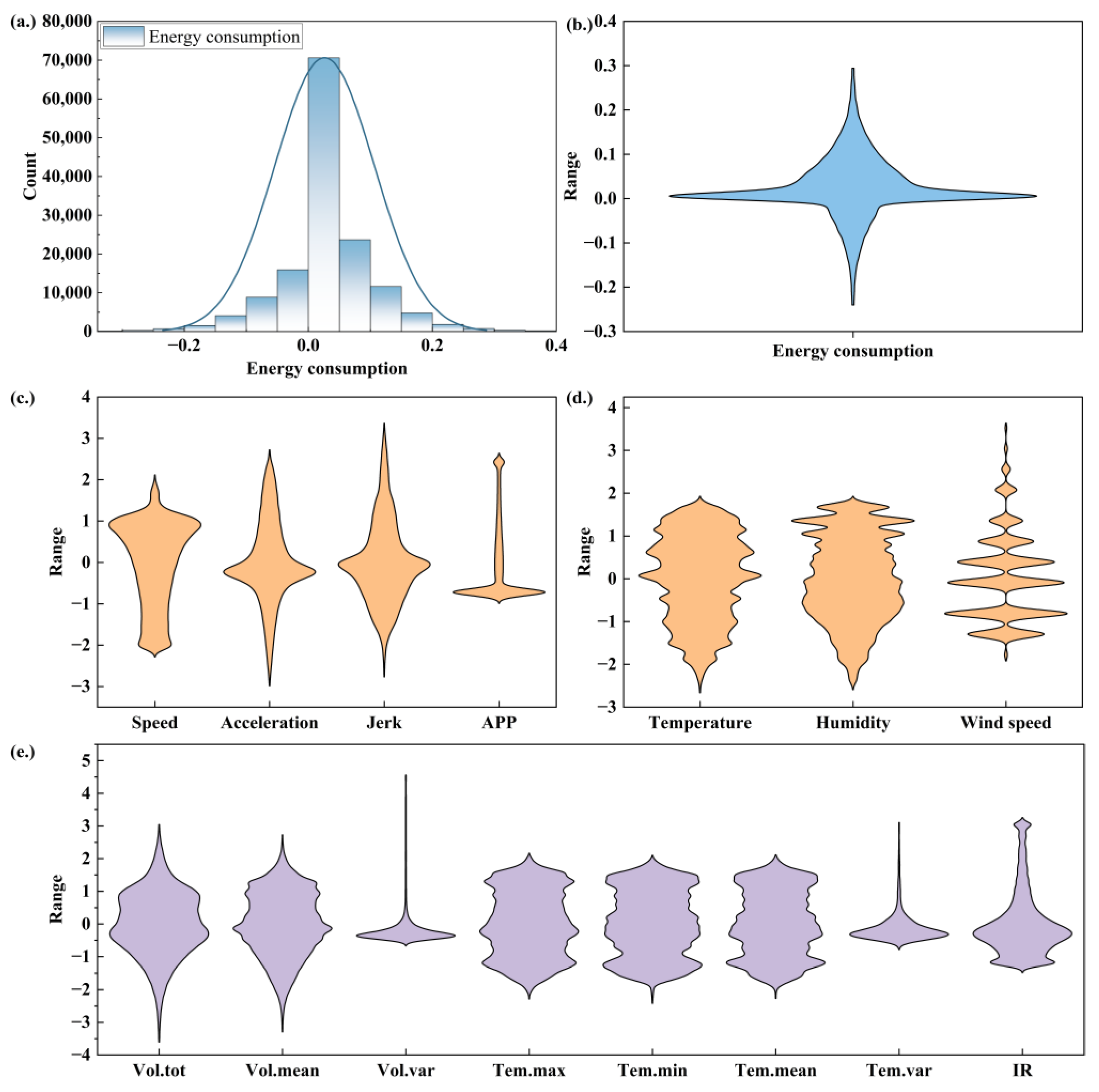
Figure 5 illustrates the spatial distribution of battery energy consumption and its influencing factors. Figure 5a,b illustrate the distribution of battery energy consumption, revealing that the data exhibit characteristics of a normal distribution, primarily concentrated around zero. Most samples exhibit energy consumption values close to zero, suggesting that vehicles predominantly operate in a low-energy consumption state during operation or under various conditions. As depicted in the histogram and violin plot, data frequency is highest around zero and gradually decreases as energy consumption values deviate from zero. The rightward extension of the kernel density estimation (KDE) curve suggests occasional periods of significant fluctuations in battery energy consumption. These higher energy consumption values, although less frequent, correspond to specific conditions in which the battery operates under high load or experiences abnormal functioning, resulting in a substantial increase in energy consumption. The occurrence of negative energy consumption on the left side of the distribution, although less frequent than that on the right side, suggests that vehicles may recover energy via the regenerative braking system under specific conditions.

Figure 5c–e presents the descriptive statistics of the factors influencing energy consumption, with all variables standardized prior to the analysis to ensure dimensional consistency. In terms of driving characteristics, Speed and Acceleration exhibited relatively dispersed distributions, indicating considerable variability among the samples, whereas APP demonstrated a more concentrated distribution, suggesting smaller fluctuations. Temperature and humidity exhibited relatively symmetric distributions. In contrast, wind speed displayed a distinctly multimodal distribution that gradually narrows at both ends, indicating that extremely high or low wind speeds occur less frequently. Regarding battery parameters, Vol. tot has a wide distribution range, suggesting significant fluctuations in the battery load over different time periods. Vol. mean also exhibits a broad distribution, while Vol. var remains relatively concentrated, implying that although the overall voltage level of the battery system varies considerably under different conditions, the voltage differences among individual sub-batteries remain relatively stable. Similarly, both Tem. mean and Tem. var indicate substantial temperature variations under different operating conditions, while the internal temperature differences among the sub-batteries remain stable. Tem. max and Tem. min exhibited broad and symmetric distributions, suggesting significant variations in the extreme battery temperatures across different scenarios. IR remains relatively concentrated for most of the time; however, its wide range of fluctuations implies that the battery’s insulation resistance may undergo considerable variation under different operating states.

5.2. Hyperparameter Optimization and Prediction Performance Comparison

To enhance the predictive performance and generalization ability of both the stacking and surrogate models, a two-stage hyperparameter optimization strategy was adopted in this study. In the first stage, a grid search combined with 5-fold cross-validation was applied to each of the three base learners in the first layer of the stacking model to determine the optimal values of n_estimators, max_depth, and learning_rate. In the second stage, the surrogate model was also tuned using a grid search with 5-fold cross-validation, targeting the optimization of n_estimators, learning_rate, max_depth, and the subsampling ratio subsample. The final optimal parameter configurations are listed in

Table 5. The results of hyperparameter optimization.

Parameter	Values	Description
n_estimators	140	The number of decision trees in the RF
	150	The number of decision trees in the GBDT
	150	The number of decision trees in the CatBoost
	200	The number of decision trees in the XGBoost
Learning-rate	0.1	The Learning-rate in the GBDT
	0.1	The Learning-rate in the CatBoost
	0.1	The Learning-rate in the XGBoost
max_depth	10	The maximum depth of the tree in RF
	5	The maximum depth of the tree in GBDT
	7	The maximum depth of the tree in XGBoost
depth	6	The maximum depth of the tree in CatBoost

.

To comprehensively evaluate the fitting accuracy of the model for battery energy consumption prediction, this study employs three widely used statistical metrics: mean squared error (MSE), mean absolute error (MAE), and root mean squared error (RMSE), with their respective calculation formulas defined in Equations (11)–(13). Among them, MSE and RMSE apply a squared transformation to the error terms, assigning greater weight to larger deviations, thereby making the evaluation more sensitive to instances with high errors. In contrast, the MAE calculates the average of the absolute deviations between the predicted and actual values, offering results with clear physical meaning and ease of interpretation. By incorporating both absolute and squared error metrics, this study evaluates the model’s accuracy and robustness from multiple perspectives, providing a solid foundation for formulating subsequent energy management strategies.

$$MSE={\displaystyle \frac{1}{n}}{\sum }_{i=1}^n{(y_i-{\widehat{y}}_i)}^2,$$

(11)

$$MAE={\displaystyle \frac{1}{n}}{\sum }_{i=1}^n{|y}_i-{\widehat{y}}_i|,$$

(12)

$$RMSE=\sqrt{{\displaystyle \frac{1}{n}}{\sum }_{i=1}^n{(y_i-{\widehat{y}}_i)}^2}$$

(13)

To further validate the effectiveness of the proposed stacking model, it is compared with several representative models. Specifically, the base learners of the stacking model included various ensemble algorithms, such as RF, CatBoost, and GBDT. These models, as typical representatives of machine learning approaches, demonstrate strong generalization capabilities in similar prediction tasks. In addition, deep learning models such as CNN and RNN have been widely applied in the field of energy consumption prediction in recent years; therefore, selected deep learning models are also included for comparison. By evaluating the performance of the stacking model against both traditional machine learning models and state-of-the-art deep learning approaches, this study aims to provide a comprehensive assessment of the predictive advantages and robustness of the proposed method.

As shown in

Table 6. Comparison of prediction results from different models.

	MSE	RMSE	MAE
AdaBoost	0.0030	0.0548	0.0328
RF	0.0024	0.0486	0.0279
GBDT	0.0025	0.0496	0.0262
CatBoost	0.0028	0.0529	0.0288
CNN	0.0023	0.0477	0.0288
DNN	0.0027	0.0518	0.0336
RNN	0.0024	0.0491	0.0297
Stacked models	0.0020	0.0444	0.0241
Surrogate model	0.0020	0.0445	0.0242

, the stacked model outperforms all baseline models, achieving the lowest MSE (0.0020), RMSE (0.0444), and MAE (0.0241). This demonstrates that the stacking framework, which integrates multiple base learners through a meta-model, offers superior predictive accuracy and generalization ability. Moreover, the surrogate model—trained to approximate the output of the stacked model—achieves nearly identical performance, indicating its strong ability to replicate the behavior of the ensemble. Compared with conventional machine learning and deep learning models, the stacked model and its surrogate show clear advantages across all evaluation metrics, confirming the effectiveness of the stacking strategy.

5.3. Overall Feature Contribution Analysis

To analyze the impact mechanism of various influencing factors on battery energy consumption, this study applies the SHAP framework to evaluate both the direction and magnitude of each factor’s effect on the dependent variable. Figure 6 presents the feature importance scatter plot and bar chart generated using the SHAP model. Figure 6a shows the distribution of the SHAP values for each feature across all samples. The color represents the feature value for each sample (red indicates high values and blue indicates low values), while the horizontal spread of the points reflects the degree to which each sample influences battery energy consumption. This plot also reveals the overall direction of each feature’s effect on the target variables. Figure 6b ranks the features by importance and presents their average impact on battery energy consumption, which is quantified by the mean absolute SHAP value. By jointly analyzing both plots, we can assess not only the relative importance of each variable but also the direction of its influence, providing an intuitive understanding of the internal mechanism of the stacking model.

Based on the above results, this study quantified the overall relative importance of the three major categories of features in relation to battery energy consumption, as shown in

Table 7. Overall contribution of feature categories to energy consumption.

Feature Category	|Collective Contribution|
Battery System	56.5%
Driving characteristics	42.3%
Environmental Data	1.2%

. In addition, to focus on the most representative influencing factors, the study extracted the relative importance of the ten most impactful features, as shown in Figure 7. The percentage values in the figure indicate the relative contribution of each feature to the model’s prediction, while the colors represent the categories to which the features belong. These features contribute most significantly to the model output and play a dominant role in determining the battery energy consumption. Analyzing these key features enables a more targeted understanding of the underlying mechanisms and provides recommendations for optimizing energy efficiency.

In the model, battery system indicators exerted the most substantial influence on energy consumption, with a cumulative contribution of 56.5%. From a macro perspective, Vol. tot is one of the primary driving factors, contributing −28.32% in total and ranking second among all variables. Vol. mean contributes 22.33%, indicating that higher average voltage levels lead to increased energy consumption. This suggests that while a moderate overall voltage level supports energy efficiency, an excessively high average voltage may hinder energy consumption control. Vol. var, which contributed 3.62%, underscores the importance of regulating the internal voltage distribution differences within the battery system. The IR contributed −0.71%, implying that strong insulation performance helps suppress leakage losses and enhances the overall system efficiency. Tem. var, with a contribution of 0.57%, further indicates that an uneven temperature distribution can intensify localized thermal effects, leading to increased energy consumption and underscoring the need for effective thermal management. Overall, maintaining an appropriate total voltage level, improving voltage stability, ensuring reliable insulation performance, and optimizing thermal management strategies are key measures for reducing the energy consumption.

Driving characteristics significantly impact battery energy consumption. Among them, APP (30.92%), acceleration (6.38%), speed (−4.01%), and jerk (1.02%) are the major contributing features, collectively accounting for 42.3% of the total contribution. This result indicates that aggressive acceleration and unstable driving behaviors notably increase energy consumption. Specifically, APP ranks first among all features in terms of contribution, highlighting its critical role as a driving factor of battery energy usage. A higher APP value reflects more intense acceleration behavior, requiring the battery to deliver a higher power output to meet driving demands, thereby increasing energy consumption. Similarly, increases in acceleration and jerk intensify the instantaneous power demand, elevate the battery load, and accelerate energy loss. In contrast, the negative contribution of speed suggests that maintaining a moderate and stable driving speed improves battery system efficiency and reduces energy consumption. Overall, these findings underscore the importance of optimizing driving behavior and minimizing abrupt operations to enhance the energy efficiency.

Environmental data contribute a total of 1.2% to battery energy consumption, with temperature being the only environmental factor among the top ten features, contributing −0.58%. This result suggests that although environmental factors have a limited overall impact, temperature still plays a positive role in reducing battery energy consumption. Favorable ambient temperatures help decrease internal battery resistance and improve charging and discharging efficiencies, thereby reducing energy demand to some extent. These findings highlight the important role of temperature in optimizing the operating conditions of batteries.

5.4. Variables Association Analysis

Section 5.3 provides an intuitive illustration of the average contribution of each feature to battery energy consumption, which facilitates the identification of key influencing factors. However, it does not capture how variations in feature values affect the direction and magnitude of their contributions. In real-world driving scenarios, feature variables often exhibit nonlinear influence patterns and complex interactions, making average contribution values insufficient for revealing their dynamic behavior. Therefore, this study introduces SHAP dependence plots to depict the marginal impact trends of key variables across different value ranges, thereby offering a more comprehensive understanding of the factors that affect battery energy consumption. In the SHAP dependence plots, the horizontal axis represents the independent variable influencing battery energy consumption, with units consistent with those in Table 4. The vertical axis indicates the extent of the variable’s impact on the battery energy consumption, expressed as the SHAP values. Since SHAP values reflect the relative contribution of each feature to battery energy consumption, they are presented as unitless standardized explanatory metrics. In addition to visualizing the relationship between SHAP and feature values, the SHAP dependence plots also display, on the secondary vertical axis, the variable that exhibits the strongest interaction with the current feature along with its corresponding value, thereby facilitating the analysis of how feature interactions affect energy consumption.

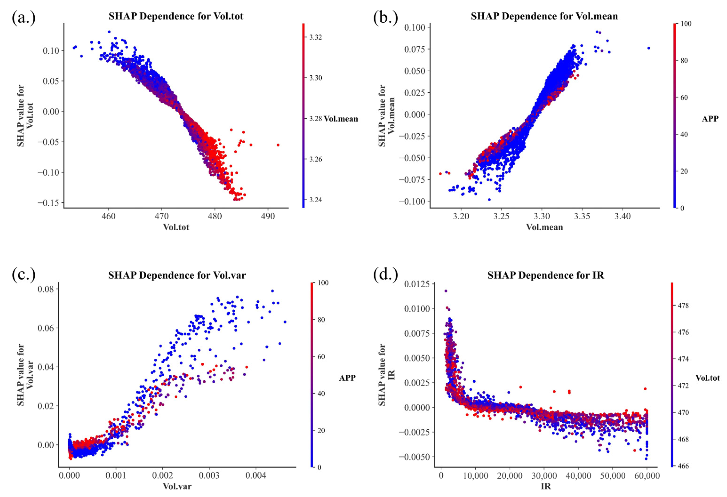
Figure 8 illustrates the marginal effects of four battery system parameters, Vol. tot, Vol. mean, Vol. var, and IR, on battery energy consumption using SHAP dependence plots, along with their interactions with key auxiliary features. The SHAP dependence plot for Vol. tot shows a clear negative correlation. The SHAP value transitions from positive to negative at approximately Vol. tot ≈ 473, indicating that when the total voltage is below this threshold, it contributes to increased energy consumption, whereas beyond this point, it helps to suppress the energy use. Furthermore, the interaction effect reveals that higher values of Vol. mean on both sides of the threshold tend to dampen the impact of Vol. tot on energy consumption—pulling the SHAP values toward zero. This suggests a moderating effect, where Vol. tot and Vol. mean jointly influence energy consumption in a compensatory way. Vol. mean exhibited a positive correlation with the SHAP values, with the SHAP value crossing zero at approximately Vol. mean = 3.28, indicating this point as a critical threshold where the contribution to energy consumption shifted from negative to positive. The interaction effect with APP is particularly prominent, and higher APP values tend to weaken the influence of Vol. mean on battery energy consumption, pulling the SHAP values closer to zero. Vol. var shows an overall upward trend in its SHAP values, with a marked increase observed when Vol. var exceeds 0.001, indicating that greater voltage fluctuations in this range lead to significantly higher energy consumption. When Vol. var is below 0.001, the SHAP values change more gradually but exhibit two distinct inflection points, suggesting a more complex nonlinear impact on energy consumption in this interval. Nonetheless, Vol. var values below 0.001 are generally associated with a suppressive effect on energy use, which provides meaningful insights for designing energy control strategies at the battery system level. APP is again identified as the most significant interacting variable. When Vol. var < 0.001, higher APP values tended to shift the SHAP values from negative to positive, indicating increased energy consumption. Conversely, when Vol. var > 0.001, higher APP values tended to suppress the increase in SHAP values, thereby mitigating the negative impact of voltage variance. IR exhibits a typical pattern of diminishing marginal effects, with its SHAP value generally decreasing as IR increases. However, this downward trend is non-linear, showing a distinct “steep-then-gradual” pattern. Notably, IR ≈ 5000 corresponds to a turning point in the rate of SHAP value change, indicating a critical threshold at which the marginal impact intensity begins to shift. In addition, IR ≈ 10,650 marks the point at which the SHAP value crosses zero, signifying a change in the direction of IR’s influence on energy consumption—from a slight positive contribution to a negative (i.e., suppressive) effect. These two critical points represent the inflection of IR’s marginal effect and the directional shift in its impact, offering valuable insights into the relationship between the insulation condition of the battery system and its energy performance.

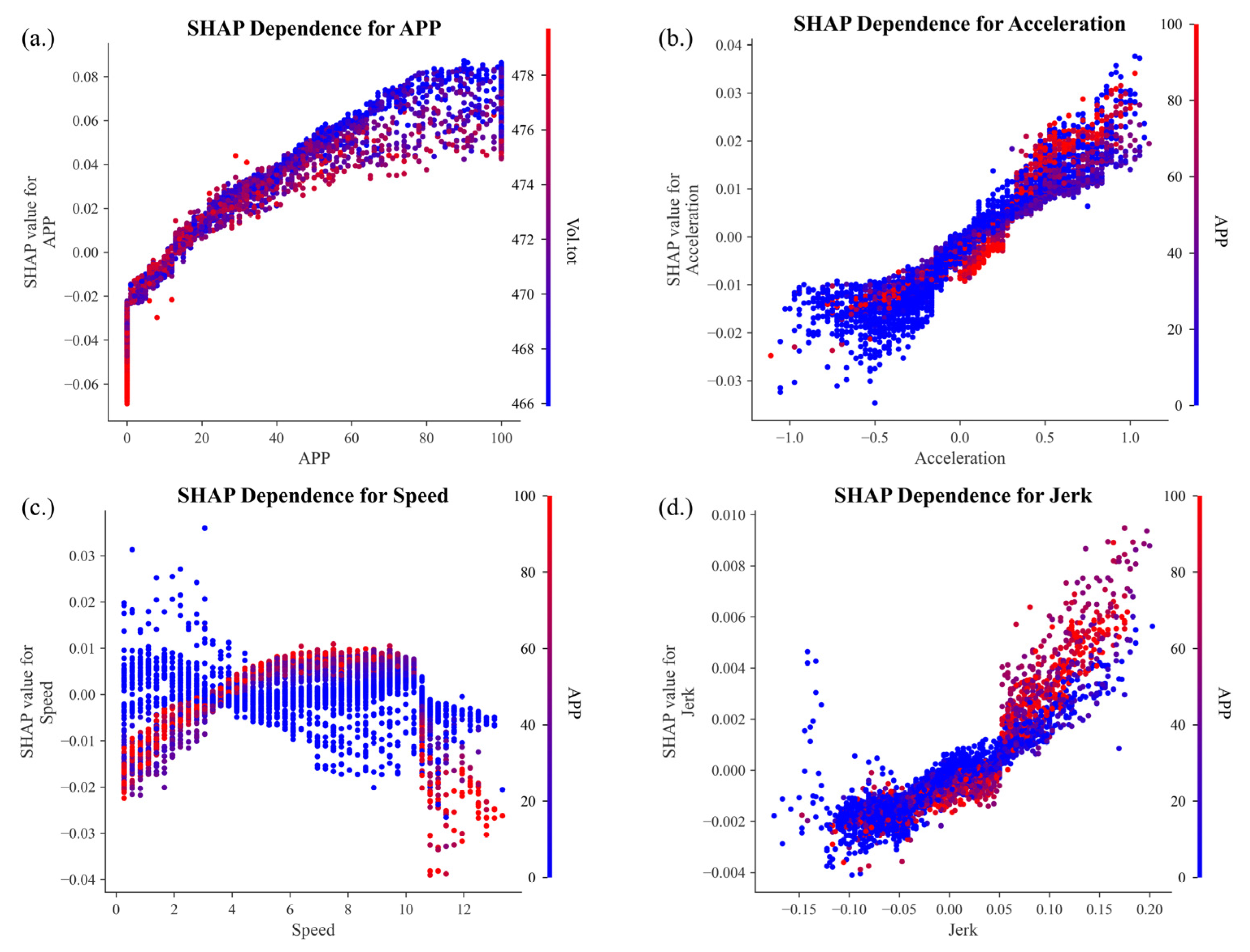
Figure 9 shows the SHAP dependence plots of the key driving-related features. The SHAP value for APP shows a monotonically increasing trend, with the rate of increase gradually slowing as APP rises. The SHAP value crosses from negative to positive at approximately APP ≈ 15, indicating that in the low throttle range, the APP has little to no impact on energy consumption and may even exert a slight suppressive effect. However, once the APP exceeds this threshold, it contributes significantly to increased energy consumption. Vol. tot demonstrates the most prominent interaction with APP. Notably, when the APP exceeds 50, higher Vol. tot values are associated with reduced SHAP values, suggesting that an elevated total voltage can mitigate the energy consumption impact of aggressive throttle inputs in higher APP ranges. The SHAP value for Acceleration exhibits an overall linearly increasing trend, transitioning from negative to positive around Acceleration ≈ 0. This indicates that positive acceleration is a major contributor to the increased energy consumption. In terms of interaction effects, the APP emerged as the primary interacting variable, with a pronounced amplification effect observed, particularly in the region where Acceleration > 0.35. In this range, higher APP values significantly increase the SHAP values of Acceleration, thereby reinforcing its positive contribution to energy consumption. This trend suggests that aggressive acceleration behavior driven by high APP inputs results in heightened energy sensitivity and elevated consumption risk. Accordingly, this region can be regarded as a critical intervention zone for energy management and control. Implementing measures to limit aggressive driving behavior or promote smoother acceleration in this region could effectively enhance overall energy efficiency. The relationship between Speed and SHAP value exhibits a parabolic pattern—initially increasing and then decreasing—with significant differences in interaction effects across various speed ranges. Specifically, in both the low-speed range (approximately 0–4 m/s) and the high-speed range (above 10 m/s), lower APP values are associated with higher SHAP values. In the moderate speed range (approximately 4–10 m/s), SHAP values remain at a relatively high level, and higher APP values further amplify the SHAP values. This trend indicates that aggressive driving behavior significantly intensifies the energy consumption within the moderate speed range. Jerk shows a positive correlation with SHAP values, indicating that the smoothness of driving behavior has a significant impact on energy consumption. The SHAP value increases notably when Jerk > 0, suggesting that sudden acceleration or unsteady driving substantially increases energy consumption.

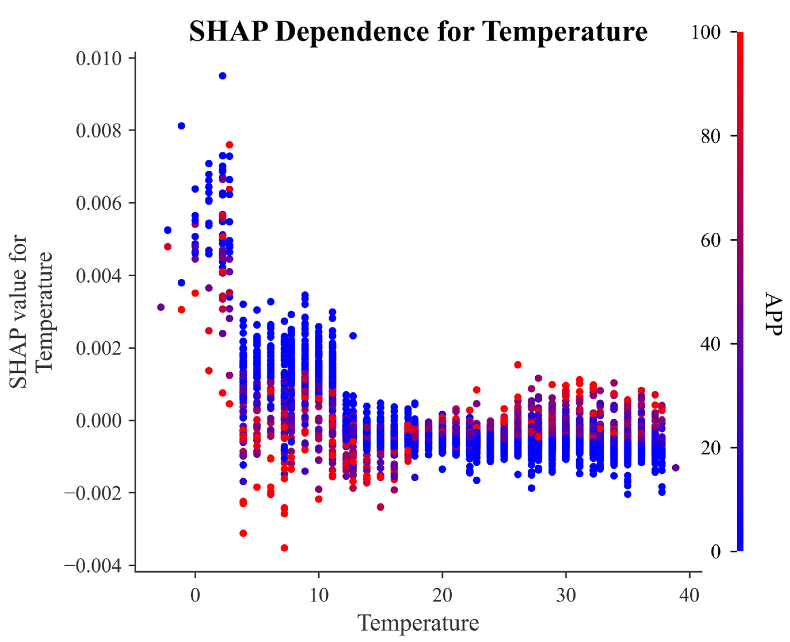
Figure 10 illustrates the SHAP dependence of Temperature on battery energy consumption. Overall, Temperature exhibits a clear negative correlation with SHAP values. A critical threshold is observed at approximately 13 °C, where the SHAP value shifts from positive to negative. This indicates that lower ambient temperatures are associated with higher energy consumption during vehicle operation, which may be attributed to increased use of heating systems and changes in battery electrochemical activity under cold conditions. This finding highlights the importance of enhancing the adaptability of energy management strategies in low-temperature environments. In particular, incorporating temperature-aware energy consumption prediction and optimization mechanisms is essential to improve the operational efficiency and range stability of battery systems under varying climate conditions.

In summary, this section reveals the marginal contribution patterns and interaction effects of key features from three categories of data on battery energy consumption. By identifying the nonlinear influence pathways and critical threshold transitions of these features, the analysis facilitates a deeper understanding of how different variables affect energy consumption under complex operating conditions. Moreover, the findings provide a theoretical foundation for the development of future energy-optimization and control strategies.

6. Conclusions and Future Work

6.1. Conclusions

This study, based on a framework integrating stacking models, surrogate models, and SHAP analysis, predicts the operational energy consumption of electric buses and investigates the key influencing factors and their underlying mechanisms. The results show that battery operational parameters, driving characteristics, and environmental factors contribute 56.5%, 42.3%, and 1.2% to energy consumption prediction, respectively. Among them, battery parameters such as Vol. tot, Vol. mean, Vol. var, and IR have the most significant impact on energy consumption. In terms of driving characteristics, APP, Acceleration, Speed, and Jerk are identified as critical influencing factors. Among the environmental variables, ambient temperature exerts the most notable effect. This study also identifies the nonlinear influence patterns of these key features, which enhances the understanding of how they affect battery energy consumption and offers new perspectives for promoting energy conservation, emission reduction, and sustainable development in transportation systems. Based on the above findings, this study proposes the following optimization recommendations to improve the energy efficiency of electric buses:

(1)

Optimizing the Battery Management System (BMS) to improve energy utilization efficiency. SHAP analysis reveals that a higher Vol. tot is significantly associated with lower energy consumption, particularly when Vol. tot exceeds 473, where the SHAP value tends to be negative, emphasizing the importance of maintaining a stable and efficient overall voltage level during operation. Meanwhile, the positive contributions of Vol. mean and Vol. var indicate that controlling voltage fluctuations and ensuring voltage stability are equally crucial for controlling energy consumption. Specifically, when Vol. mean is below 3.28, the SHAP value is less than 0, indicating that the average voltage range is associated with lower energy consumption. When the Vol. var is below 0.001, the SHAP value is relatively low, suggesting that a more uniform voltage distribution helps reduce energy consumption. Additionally, IR is identified as a key variable, with its marginal effect indicating that when IR exceeds 10,650, the SHAP value becomes negative, highlighting the importance of improving insulation quality to enhance energy efficiency. Therefore, optimizing the BMS should go beyond mere passive state monitoring and incorporate proactive regulation and predictive control capabilities. Specifically, the BMS should implement dynamic voltage regulation strategies to ensure that Vol. tot and Vol. mean remain within energy-efficient operating ranges. Moreover, real-time monitoring and rapid response mechanisms are beneficial for mitigating energy fluctuations related to Vol. var. Regular assessment of insulation conditions and timely identification of potential faults are also crucial for further ensuring the efficient, safe, and low-carbon operation of battery systems.

(2)

Given the significant impact of driving characteristics on battery energy consumption, this study confirms that targeted adjustments to driving behavior are essential for controlling energy usage. The results indicate that aggressive acceleration, characterized by high APP values, significantly increases energy consumption, whereas smooth acceleration and moderate throttle input can effectively alleviate this burden. The positive correlations between Acceleration, Jerk, and energy consumption further suggest that gradual speed changes and smooth velocity transitions help reduce energy demands during dynamic driving conditions. These findings underscore the necessity of employing intelligent driver-assistance systems to suppress extreme driving behaviors, such as sudden starts and stops, thereby enhancing overall driving stability and facilitating energy control. Additionally, the adverse impact of high APP values within the moderate-speed range should not be overlooked. In conclusion, refined management of driving behavior can significantly reduce the operational energy consumption of electric buses and support the development of more sustainable urban transportation systems.

(3)

The study finds that among various environmental factors, temperature is one of the primary variables affecting battery energy consumption, with its impact being particularly evident under extreme climate conditions. Such extreme temperatures are typically associated with increased energy demand, especially due to the operation of auxiliary systems like air conditioning. The results highlight the importance of enhancing the energy adaptation capabilities of vehicles under these conditions. Specifically, optimizing the energy management strategy of the air conditioning system and implementing battery preheating mechanisms in low-temperature environments can help mitigate the negative effects of ambient temperature fluctuations on battery performance and the overall energy consumption of the vehicle.

6.2. Limitations and Future Work

Despite the valuable findings of this study, several limitations remain. First, the training process of the stacking model is relatively complex, requiring substantial computational resources and posing challenges for parameter tuning, which may limit its practical applications. Secondly, this study was validated only in Changsha, Hunan Province, China. Future research should consider extending model validation to a broader range of geographical regions or datasets to assess its generalizability under different geographic and climatic conditions. In addition, the indicator system constructed in this study still has room for further expansion. For example, vehicle load is an important factor that should be prioritized and incorporated into future indicator systems. However, due to data limitations, this study was unable to obtain the real-time load data of electric buses during operation. Although vehicle load does not directly affect speed, acceleration, or environmental variables, it can significantly influence motor load, thereby impacting overall energy consumption. Therefore, future research should consider incorporating real-time load and other supplementary data and gradually transition from the current offline testing to online testing, in order to further enhance the model’s accuracy and comprehensiveness in predicting energy consumption and analyzing its influencing mechanisms.