Abstract
This study presents an integrated geospatial framework for assessing the risk to high-speed railway (HSR) infrastructure, combining a persistent scatterer interferometric synthetic aperture radar (PS-InSAR) analysis with multi-criteria decision-making in a geographic information system (GIS) environment. Focusing on the Honam HSR corridor in South Korea, the model incorporates both maximum ground deformation and subsidence velocity to construct a dynamic hazard index. Social vulnerability is quantified using five demographic and infrastructural indicators, and a two-stage analytic hierarchy process (AHP) is applied with dependency correction to mitigate inter-variable redundancy. The resulting high-resolution risk maps highlight spatial mismatches between geotechnical hazards and social exposure, revealing vulnerable segments in Gongju and Iksan that require prioritized maintenance and mitigation. The framework also addresses data limitations by interpolating groundwater levels and estimating train speed using spatial techniques. Designed to be scalable and transferable, this methodology offers a practical decision-support tool for infrastructure managers and policymakers aiming to enhance the resilience of linear transport systems.
1. Introduction
High-speed railways (HSRs) are essential for achieving sustainable and low-carbon urban mobility, enabling rapid interregional connectivity. However, due to their extended linear geometry and rigid infrastructure, HSR systems are highly vulnerable to ground deformation, particularly in geologically unstable or reclaimed terrains. In South Korea, the Honam HSR corridor traverses floodplains and soft alluvial zones with high subsidence potential, making it a critical subject for risk monitoring [1,2].
Persistent scatterer interferometric synthetic aperture radar (PS-InSAR) is widely recognized as a reliable remote sensing technique for detecting millimeter-scale surface displacement over long temporal and spatial ranges [3,4]. Beyond geophysical deformation monitoring, recent studies have extended the application of InSAR to other risk-related domains, such as air quality and disaster impact assessment. For example, ref. [5] demonstrated the integration of InSAR coherence with atmospheric satellite observations to examine air quality deterioration in conflict zones, while ref. [6] proposed a framework for interpreting complex subsidence mechanisms using cross-heading PS-InSAR data. These developments underscore the methodological versatility and cross-domain applicability of InSAR-based approaches, particularly in environmental and geohazard contexts.
However, while PS-InSAR provides precise geophysical data, it does not directly assess whether such displacements pose a functional risk to infrastructure or human settlements. Several studies have attempted to bridge this gap by integrating InSAR outputs with GIS-based risk modeling frameworks, particularly in urban environments [7,8]. Nevertheless, these models typically focus on general hazard mapping and rarely address the unique requirements of high-speed railways, which demand infrastructure-specific spatial resolution and operational decision-making logic.
Multi-criteria decision-making (MCDM) methods such as the analytic hierarchy process (AHP) have become increasingly popular for integrating diverse hazard and vulnerability indicators in geospatial risk assessments [9,10]. Studies have applied AHP–GIS frameworks to assess various natural hazards such as floods [11], landslides [12], and waterlogging [13]. However, these models often overlook two critical limitations: (1) the dynamic spatiotemporal characteristics of ground deformation, and (2) potential interdependencies among indicators, which can distort weight estimation in conventional AHP models [14].
To overcome these limitations, this study proposes an integrated spatiotemporal risk modeling framework tailored to high-speed railway corridors in smart urban environments. Our model combines millimeter-level vertical deformation data derived from PS-InSAR with ten key indicators: five representing geotechnical and operational hazards (e.g., maximum deformation, subsidence rate, groundwater depletion, track type, and train speed), and five reflecting socio-environmental vulnerability (e.g., population density, GDP, urbanization rate, vulnerable population ratio, and emergency service accessibility). Each indicator is systematically weighted using a two-stage AHP approach and further refined using Euclidean distance-based dependency correction to reduce redundancy and enhance analytical robustness.
The proposed model generates a high-resolution, segment-level composite risk map that enables infrastructure managers and policymakers to prioritize maintenance, implement early warning systems, and formulate long-term resilience strategies. By linking deformation patterns with socioeconomic exposure, this study provides a practical and scalable solution for risk-informed planning in high-speed railway systems.
Furthermore, our framework contributes meaningfully to the evolving discourse on smart urban corridors by integrating physical hazard data and urban vulnerability indicators into a GIS-based decision-support system tailored for linear infrastructure risk assessment. The proposed methodology is not only spatially explicit and segment-sensitive but also designed to be transferable across different types of transport corridors and adaptable to diverse geographic and data environments. This adaptability ensures the framework’s utility as a practical tool for future urban resilience planning and mobility management.
Previous studies have conceptualized smart corridors as integrated urban infrastructures that combine ecological restoration with digital governance [15,16], serve as testbeds for smart environmental experimentation [16], or function as spatial strategies for achieving smart sustainability goals [17,18,19]. Additionally, smart corridors have been recognized as platforms for participatory planning and urban governance [20,21], as well as mechanisms for enhancing resilience in metropolitan peripheries [22,23].
In alignment with these perspectives, this study defines a “Smart Urban Corridor” as an integrated infrastructure domain where high-speed transportation systems, remote sensing technologies, and GIS-based analytical tools are collectively employed to support data-informed resilience planning, infrastructure risk management, and long-term strategic maintenance prioritization.
2. Materials and Methods
2.1. Study Area
The Honam High-Speed Railway (HSR) corridor, located in the southwestern region of South Korea, spans approximately 182.3 km between Osong Station in North Chungcheong Province and Gwangju Songjeong Station in South Jeolla Province. As a major component of Korea’s high-speed rail network, the corridor supports train operations at speeds of up to 300 km/h, thereby enhancing regional integration and transportation efficiency [24].
The study area is not situated near any known active fault lines and is considered seismically stable. Although a temporary suspension of train services occurred during Typhoon Hinnamnor in 2022, the disruption was short-lived and did not result in structural damage. Historically, geotechnical issues have posed a more significant concern in this region. The Honam HSR was constructed on embankment foundations composed of mixed sand and clay, which raised concerns about ground subsidence even prior to the commencement of operations. In response, this study was supported by the Government of the Republic of Korea to assess ground deformation and associated risks along the Honam HSR using a PS InSAR-based framework. The surrounding land use is characterized predominantly by low rise residential areas, agricultural fields, and transport infrastructure, which were integrated into the spatial vulnerability assessment.
From a geotechnical standpoint, the corridor traverses broad alluvial plains underlain by weak and highly compressible soils, including clay and silt layers. These subsurface conditions are prone to long-term consolidation and differential settlement, posing structural challenges to rail infrastructure stability. According to [24], such ground conditions represent one of the principal risk factors contributing to uneven deformation along the corridor.
In addition to geotechnical characteristics, climatic and topographic conditions play a significant role in shaping ground deformation risks along the corridor. The study area experiences seasonal variations in rainfall and temperature, which contribute to soil moisture fluctuation and thermal expansion–contraction cycles. Moreover, the elevation profile varies from low-lying floodplains to gently undulating terrain, influencing surface runoff and subsurface water dynamics. These environmental factors are important contextual elements for interpreting the deformation patterns captured through PS-InSAR.
Empirical evidence underscores the significance of this concern. Following the line’s inauguration, ground deformation monitoring programs detected vertical subsidence in approximately 16 percent of the total corridor length, with maximum vertical displacements reaching up to 5.6 cm in critical embankment zones [25,26]. These observations highlight the importance of continuous subsidence surveillance and risk mitigation, particularly in sections where ground conditions and infrastructure types are heterogeneous.
Structurally, the Honam corridor incorporates a range of engineering forms, including embankments, cuttings, viaducts, and tunnels, with each exhibiting distinct sensitivity to ground deformation. The predominant use of concrete slab tracks offers high geometric stability but may amplify deformation stress, while shared segments with conventional rail utilize ballasted tracks that respond differently to subsurface movement. These variations necessitate differentiated modeling of infrastructure vulnerability.
The present study applies a persistent scatterer interferometric synthetic aperture radar (PS InSAR) analysis along the entire Honam High-Speed Railway corridor to quantify ground subsidence and generate a spatial risk map using the analytic hierarchy process (AHP). The corridor includes critical segments such as Gongju, Iksan, and Sintaein, where previous reports documented vertical displacements of up to 5.6 cm, affecting approximately 16 percent of the total alignment, primarily due to weak alluvial deposits [24]. To provide a more recent and detailed assessment, this study utilized 29 high-resolution X-band SAR images acquired from TerraSAR X and TanDEM X satellites between August 2016 and September 2018. The PS InSAR analysis revealed vertical subsidence ranging from 1.56 mm to 46.47 mm across the corridor, capturing both localized and progressive deformation patterns.
Figure 1 illustrates the spatial extent of the study area along the Honam High-Speed Railway corridor, encompassing the full alignment from Osong Station in the north to Songjeong Station in the south. The yellow polygon delineates the designated smart urban corridor, which serves as the primary focus of this analysis.
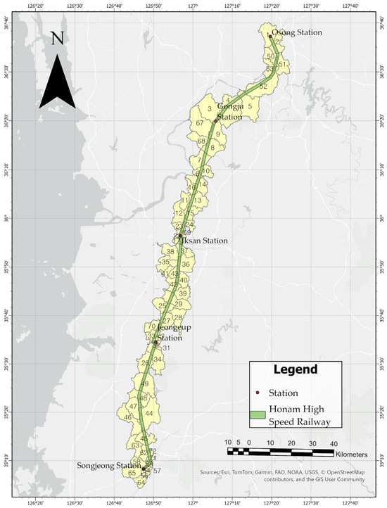
Figure 1.
Spatial extent of the Honam High-Speed Railway (HSR) corridor from Osong Station to Songjeong Station. The map shows the high-speed railway alignment (green line), station locations (red dots), and the Smart Urban Corridor area (yellow polygon) used as the study boundary. The figure number is represented in Appendix B, Figure A12 and Table A6.
2.2. Data Collection
2.2.1. Collection of Satellite Imagery for PS InSAR Analysis
To quantify long-term ground deformation along the Honam High-Speed Railway corridor, this study employed the persistent scatterer interferometric synthetic aperture radar (PS InSAR) technique, as established in prior studies [1,27,28].
The derived deformation measurements were geocoded and interpolated into 5 m resolution raster datasets using the inverse distance weighting (IDW) method. These rasters were subsequently classified into 10 categories and visualized using ArcGIS Pro 3.5, forming the core input for spatial risk analysis. Validation was conducted using ground control points (GCPs) and known subsidence-prone areas, yielding a root mean square error (RMSE) of less than 2 mm per year, consistent with the accuracy levels reported in previous PS InSAR studies on linear infrastructure.
By integrating high-resolution ground deformation data into a GIS-based analytical framework, this approach offers practical geospatial insights for smart urban corridor planning, with direct implications for predictive maintenance strategies and resilient infrastructure design.
The dataset comprised 29 high-resolution X-band SAR images, including 24 TerraSAR-X and 5 TanDEM-X acquisitions, obtained between August 2016 and September 2018. All scenes were acquired in ascending right-looking mode with HH polarization. The StripMap products used in this study have a spatial resolution of approximately 3 m in range and 3.3 m in azimuth. A master image dated 23 October 2017 was selected for interferogram generation. It is noteworthy that no SAR acquisitions were possible between June and September 2017 due to restricted satellite tasking caused by heightened security surveillance over the Korean Peninsula following multiple missile tests and North Korea’s sixth nuclear test on 3 September 2017.
The final acquisition in this dataset, dated 4 October 2018, is illustrated in Appendix C (see Figure A13 and Figure A14), showing the precise SAR footprint over the study area. All satellite images were commercially procured from Airbus Defence and Space, and researchers may contact the corresponding author for potential data sharing upon request.
To capture the full 188 km span of the Honam High-Speed Railway (HSR), a total of four SAR scenes were acquired using TerraSAR-X and TanDEM-X satellites. To enhance spatial coherence and detail, each scene was subdivided into overlapping segments—specifically, Scene 1-1, Scene 1-2, Scene 2, Scene 3-1, Scene 3-2, Scene 4-1, and Scene 4-2—enabling continuous ground deformation monitoring along the entire corridor. This study primarily focused on the analysis results from Scene 1, while the remaining scenes (Scenes 2, 3, and 4) are provided in Appendix A for reference.
Table 1 summarizes the 29 X-band SAR images used for PS-InSAR analysis of Scene 1, which represents a key section of the Honam High-Speed Railway corridor. The dataset includes 24 TerraSAR X and 5 TanDEM X acquisitions, all collected in right-looking, ascending mode with HH polarization. Each image is characterized by its acquisition date, baseline, temporal interval, and Doppler centroid. Scenes 2 through 4, which cover the remaining sections of the corridor, are provided in Appendix A for reference.

Table 1.
Types of X-band SAR images used in this study (Scene 1).
2.2.2. PS-InSAR Processing
The persistent scatterer interferometric synthetic aperture radar (PS-InSAR) technique was employed to extract time-series ground deformation along the Honam High-Speed Railway corridor. This method identifies stable reflectors, often human-made structures such as railway tracks, bridges, and buildings, that retain high coherence over multiple SAR acquisitions. PS-InSAR is capable of detecting millimeter-scale displacement by analyzing the temporal phase stability of these persistent scatterers, as demonstrated in previous research.
The processing followed a standardized workflow (Figure 2). First, all SAR images were coregistered to a master scene to ensure pixel-level alignment across the entire image stack. Second, differential interferograms were generated by calculating phase differences associated with surface displacement, while minimizing spatial and temporal decorrelation. Third, atmospheric phase screen (APS) distortions, primarily due to tropospheric delays caused by varying weather conditions such as temperature and humidity, were mitigated using spatial filtering and temporal low-pass filtering techniques implemented in SNAP 6.0. This preprocessing step plays a critical role in reducing atmospheric artifacts that can obscure true ground deformation signals.
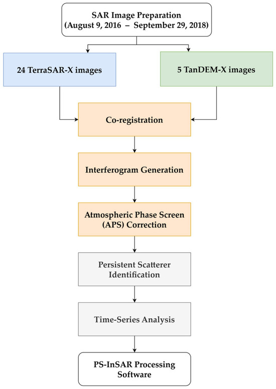
Figure 2.
Workflow of PS-InSAR processing applied in this study, including SAR image preparation, co-registration, interferogram generation, APS correction, persistent scatterer identification, and time-series analysis. The different colors represent distinct stages of the processing: blue for input data (24 TerraSAR-X images and 5 TanDEM-X images), orange for processing steps (co-registration, interferogram generation, APS correction), gray for analysis stages (persistent scatterer identification, time-series analysis), and the final step of PS-InSAR processing software at the bottom.
Fourth, persistent scatterer candidates were automatically extracted based on amplitude dispersion and phase coherence thresholds. These selected points were used to construct a stable network for time-series analysis. Finally, displacement time series were derived relative to a network of ground control points (GCPs), ensuring consistency across all observations.
To further enhance the spatial reliability and referencing accuracy of PS-InSAR measurements, a total of 17 corner reflectors were strategically installed along the railway corridor. These artificial reflectors were deployed at key segments to supplement natural PS density, particularly in vegetated or topographically complex areas, thereby improving the signal-to-noise ratio and ensuring robust phase connectivity.
Additionally, although the influence of radar lens density on signal backscattering can vary by surface material and geometry, the use of high-resolution TerraSAR-X and TanDEM-X datasets helped maintain adequate spatial sampling and signal quality along the linear railway infrastructure.
2.2.3. PS-InSAR Coregistration and Coherence
Although SAR satellites acquire imagery along repeat orbits, perfect spatial alignment between acquisitions is rarely achieved due to slight variations in sensor positioning and look angle. These temporal and spatial offsets necessitate a coregistration process to ensure pixel-level correspondence across all SAR scenes.
To achieve precise alignment, backscatter maps representing the radar return intensity are employed. These maps are generated by coregistering a single master image with multiple slave images. In this study, one master image was selected and coregistered with 28 slave images to produce a consistent set of backscatter maps for further analysis.
The resulting backscatter imagery is expressed in grayscale; brighter pixels indicate stronger radar reflectivity and darker pixels indicate lower backscatter intensity. While the reflectance characteristics vary by SAR band, certain general patterns apply: steel-framed structures, concrete buildings, and other human-made targets typically exhibit high reflectivity, whereas farmlands, barren lands, mountainous areas, and water bodies show weak backscatter. Notably, asphalt surfaces exhibit strong backscatter in the X band (used in this study) but tend to reflect weakly in L- and C-band imagery [29,30,31,32,33]. The grayscale backscatter maps used in this study are illustrated in Appendix A, Figure A1.
Coherence is a key metric used to assess the quality of SAR imagery and is computed through the coregistration of master and slave images. It quantifies the degree of similarity between two SAR acquisitions at the pixel level, with higher coherence values indicating improved interferogram quality. In PS-InSAR processing, coherence is derived by first generating reflectivity images for both the master and slave scenes, followed by the calculation of pixel-wise coherence. The coherence at a given pixel can be mathematically expressed as described in prior studies [34,35,36]:
In this equation, the following applies:
- γ is the complex coherence coefficient, representing the normalized correlation between two complex SAR signals.
- y1 and y2 denote the complex SAR signals acquired at two different observation times.
- E[·] represents the expectation operator, indicating the ensemble average or statistical mean.
- |y1|2 and |y2|2 are the squared magnitudes (power) of the respective SAR signals.
- The numerator E[y1·y2] is the cross-correlation (covariance) between the two signals.
- The denominator is the geometric mean of the power of the two signals, ensuring that the coefficient is normalized between 0 and 1.
Coherence (or decorrelation) is influenced not only by the geometric relationship between image pairs but also by spatial and temporal baselines, which can degrade coherence and consequently affect interferogram quality [37,38,39,40].
In this equation, BL represents baseline decorrelation caused by the spatial separation between satellite orbits, dop denotes Doppler decorrelation due to spectral misalignment, and vol accounts for volume-scattering effects, such as electromagnetic refraction. Thermal decorrelation arises from sensor-induced noise, temporal decorrelation results from the time interval between acquisitions, and processing refers to decorrelation introduced during interferometric processing.
In practice, most recently launched high-performance SAR satellites are capable of minimizing the majority of decorrelation sources. As a result, only spatial baseline and temporal decorrelation are typically considered significant, while other components are often assumed to be negligible in PSInSAR applications.
In this study, a Minimum Spanning Tree (MST)-based interferometric network was constructed to calculate coherence, replacing the conventional star graph configuration centered on a single master image. The MST approach establishes interferometric pairs by connecting image scenes with the shortest possible spatial and temporal baselines, thereby effectively mitigating baseline and temporal decorrelation effects.
A total of 29 TerraSAR-X and TanDEM-X images acquired over a 28-month period were used to construct the MST network, resulting in 29 nodes and 406 edges within the interferometric graph. Figure 3 illustrates the structure of the resulting MST network.
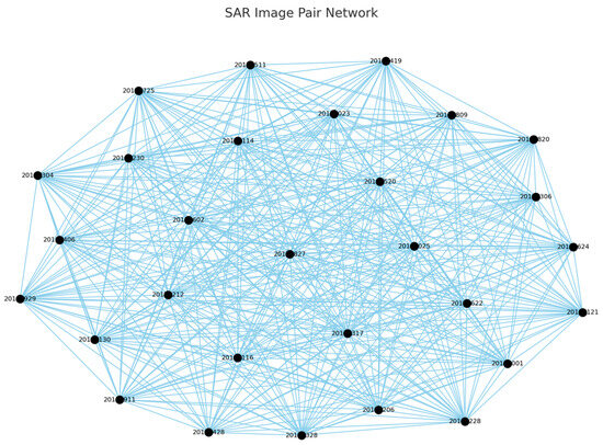
Figure 3.
Interferometric SAR network constructed from 29 acquisition dates, resulting in 29 nodes and 406 edges within the interferometric graph. Each node represents a SAR image acquisition date, and each edge denotes a potential interferometric pair.
Unlike other methods that estimate surface displacement across the entire SAR image scene, the Persistent Scatterer Interferometry (PSI) technique selectively extracts surface deformation only at high-reflectivity, temporally stable targets known as persistent scatterer candidates (PSCs). To enhance processing efficiency and maintain result accuracy, PSC selection is based on coherence-related metrics, rather than using all pixel points. Specifically, points with high-amplitude stability and spatial coherence are preselected, followed by the generation of a triangulated irregular network (TIN) to ensure spatial connectivity. While the Delaunay method is commonly used for TIN construction, alternative approaches such as the Flowered Tree or Freely Connected Network (FCN) may be applied when PSCs are sparsely or unevenly distributed, though these methods can introduce connections involving low-coherence points.
Figure 4 illustrates different network structures used for connecting Persistent Scatterer Candidates (PSCs): Figure 4a: Delaunay-based triangulation, Figure 4b: a Freely Connected Network (FCN), and Figure 4c: a real SAR scene example showing connection intensity across the azimuth-range plane.
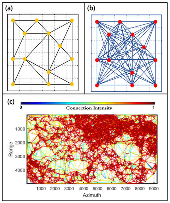
Figure 4.
Comparison of PSC point connection strategies for interferometric analysis. (a) Delaunay triangulation: a commonly used method that forms a sparse but structured network by connecting neighboring points to form triangles without overlapping edges. (b) Freely Connected Network (FCN): a denser connection strategy in which each point is connected to multiple surrounding points, increasing redundancy and network robustness, but potentially including low-coherence links. (c) Real SAR Scene Connection Map: Triangulated PSC points over a SAR scene, color-coded by connection intensity. The connection intensity ranges from low (blue) to high (red), indicating the strength and density of spatial coherence-based connections across the image in the azimuth-range domain.
The selection of persistent scatterer candidates (PSCs) is a crucial preprocessing step in PS-InSAR analysis, as it significantly affects the number, accuracy, and spatial distribution of final deformation measurements, as well as the structure and connectivity strength of the resulting triangulated irregular network (TIN). In this study, PSC selection was performed using TerraSAR-X and TanDEM-X datasets while the topographic characteristics of each study area were taken into account. In particular, for Scenes 1, 3, and 4, dense vegetation in mountainous terrain along the railway corridors caused reduced spatial coherence, increasing the potential for errors in PSC selection. To mitigate the degradation in coherence and connection strength caused by such terrain, region-specific PSC selection strategies were applied to each interferometric scene. For Scene 1, the area was subdivided into two parts due to persistently low coherence near the railway segment traversing rugged topography. Similarly, Scenes 3 and 4 were also divided into sub-regions to improve network connectivity and ensure a more robust triangulated irregular network formation. These adaptive strategies helped stabilize the PS network structure despite environmental constraints, such as vegetation cover and elevation variability.
For Scene 1, the area was subdivided into two parts due to low coherence near the railway segment traversing mountainous terrain.
- In Scene 1-1 (Cheongju Osong to Sejong), sparse point processing was applied due to limited surface exposure from tunnels. A total of 15,565 points with an amplitude stability index (ASI) ≥ 0.75 were extracted, resulting in 155,853 connections using the Local Redundant method.
- In Scene 1-2 (Buyeo to Nonsan), where flat agricultural land dominates, points were selected using a composite threshold (ASI + spatial coherence > 1.5), yielding 8290 PSCs and 82,900 connections.
Scene 2, covering Gongju to Jeongeup, features minimal topographic variation and a balanced distribution of urban and agricultural areas. It was the only scene processed as a whole, resulting in 25,147 PSCs selected with ASI ≥ 0.8 and 251,464 connections established via Closest Local Redundant linkage.
Scene 3 was also divided due to varying terrain.
- Scene 3-1 (Jeongeup downtown to Gochang) included both urban centers and adjacent rural areas. Using ASI > 0.7, 21,337 PSCs and 213,364 connections were obtained via Local Redundant connection.
- Scene 3-2 (Jangseong Buk-myeon), surrounded by steep mountains and lacking urban features, yielded only 1567 points with extremely low coherence. Here, Delaunay triangulation was adopted instead, generating 4986 links.
For Scene 4, where terrain and urban distribution varied, a similar subdivision was used.
- Scene 4-1 (Jangseong Station area) featured better PSC distribution compared to Scene 3-2 due to increased urban coverage. PSCs were selected using the ASI + spatial coherence > 1.5 criterion, with Delaunay triangulation producing 12,664 connections.
- Scene 4-2 (Jangseong to Gwangju Songjeong Station) covered both mountainous and urban areas. A total of 9549 points with ASI ≥ 0.73 were extracted and connected using Delaunay, resulting in 28,619 links.
These region-specific approaches allowed for improved coherence preservation and robust network construction tailored to the terrain and land cover characteristics of each scene.
Table 2 summarizes the number of extracted persistent scatterer candidates (PSCs), extraction and connection methods, and mean coherence values for each subdivided scene. Region-specific strategies, including amplitude-based and coherence-based selection criteria, as well as connectivity approaches (Local Redundant or Delaunay), were applied, depending on terrain characteristics and point distribution.
Table 2.
Summary of PSC extraction and connection parameters by scene.
During the study period, the ground subsidence along the Honam High-Speed Railway, as derived from PS-InSAR analysis, ranged from 1.56 mm to 46.47 mm. Each subsidence measurement was incorporated as one of the ten contributing factors in the Total Risk model, which includes five hazard indicators and five vulnerability indicators. The comprehensive PS-InSAR-derived subsidence results for the entire Honam High-Speed Railway are provided in Appendix A.
2.2.4. Hazard and Vulnerability Indicators for Spatial Risk Assessment
By integrating high-resolution deformation monitoring into a GIS-based framework, this approach provides actionable geospatial intelligence for smart urban corridor planning, particularly in supporting predictive maintenance and resilient infrastructure design.
To comprehensively assess the spatial vulnerability of the Honam High-Speed Railway (HSR) corridor, this study integrates multiple geospatial indicators representing both socioeconomic exposure and environmental sensitivity. The selection of indicators was guided by a synthesis of recent urban risk assessment frameworks in smart city contexts, particularly those using PS InSAR and AHP methodologies [41,42,43].
Five core indicators were selected to represent the vulnerability dimension: population density, vulnerable demographics, regional GDP, the urbanization ratio, and the accessibility of emergency services. These indicators reflect both the magnitude of potential social impact and the resilience of local infrastructure.
Population density and demographics: Gridded population data from the Korean Statistical Information Service (KOSIS) were used to calculate township-level density. Vulnerable populations—defined as individuals under 9 or over 65—were extracted and expressed as a demographic vulnerability ratio, normalized to a 0 to 1 scale. High-density and high-dependency zones were identified as critical exposure areas, following approaches by [5,44].
Regional GDP per capita: Economic vulnerability was quantified using local GDP data obtained from the Korean Local Economy Database. Municipal level values were log-transformed to reduce skewness and then spatially interpolated to reflect the distribution of economic assets exposed to infrastructure failure [45,46,47,48].
Urbanization ratio: Land cover data from the Environmental Geographic Information Service (EGIS) were classified to compute the urbanization ratio, defined as the proportion of built-up land (residential, commercial, industrial, and transport) in each raster cell. High urban density has been shown to correlate with elevated vulnerability to land deformation impacts, especially in transport-dependent districts [49].
Accessibility of emergency services: Geocoded data for fire stations, emergency hospitals, and ambulatory centers were retrieved from the National Spatial Data Infrastructure Portal (NSDI). Euclidean distance-based buffers were calculated to generate accessibility indices, in line with methods used in Tangshan and Shanghai urban risk models [50,51].
All variables were standardized using z-score normalization and classified into ten ordinal levels based on natural breaks (Jenks optimization), as demonstrated in recent AHP-based spatial risk assessments [52,53]. This facilitated their integration into the AHP-based multi-criteria decision model. To ensure analytical consistency and minimize multicollinearity, a correlation matrix was computed. Indicators with Pearson correlation coefficients exceeding plus or minus 0.75 were adjusted during the AHP weighting process to prevent redundancy.
These integrated socioeconomic and environmental indicators provide a detailed understanding of spatial vulnerability along the HSR corridor, supporting data-informed infrastructure planning within smart urban development frameworks.
In alignment with best practices in urban resilience assessment, our study further structures the indicator system into two primary domains: (a) regional hazard evaluation and (b) regional vulnerability evaluation. This dual-layered structure enables a more targeted interpretation of composite risk.
The hazard evaluation dimension encompasses the following five indicators:
- Maximum vertical ground deformation: derived from PS-InSAR analysis, this indicator captures the peak subsidence rate per segment, representing the most critical geotechnical hazard.
- Subsidence velocity: this refers to the average linear ground movement rate, reflecting persistent stress on infrastructure foundations.
- Groundwater depletion: based on temporal fluctuations in groundwater levels, this serves as a proxy for hydrogeological instability, commonly linked to anthropogenic extraction or seasonal stress.
- Railway segment type: each segment is classified as slab or ballast track, acknowledging differences in structural tolerance to vertical deformation.
- Design train speed: faster segments are more vulnerable to safety hazards from minor subsidence and thus require more proactive management.
In parallel, the vulnerability evaluation component includes the following five indicators:
- Population density: a higher density correlates with greater exposure in terms of potential human impact during service disruption or failure.
- Gross domestic product (GDP): used as a proxy for economic exposure; areas with a higher GDP represent greater potential losses from service interruption or asset damage.
- Urbanization ratio: reflects the proportion of built-up land, indicating physical infrastructure density and potential economic losses.
- Vulnerable demographic ratio: this quantifies populations under 15 and over 65, who are less mobile and more susceptible in emergencies.
- Accessibility of emergency facilities: proximity to fire stations, emergency centers, and medical units reflects the adaptive capacity of each area.
While many prior studies have successfully combined InSAR-derived deformation and urban vulnerability indicators to map ground-related risks in megacities such as Shanghai [42], Suzhou [54], Rome [43], and Mexico City [41], this study expands the methodological framework to the context of high-speed railway corridors, which are linear infrastructure systems that are spatially extensive yet highly localized in sensitivity. Unlike typical urban block-based zoning approaches, our model applies corridor-specific spatial granularity to capture both geotechnical hazards and socioeconomic exposure at the rail segment level.
Furthermore, by combining ground deformation patterns with regional demographic and infrastructural vulnerability, our framework delivers a high-resolution risk landscape tailored to the operational and planning needs of smart transport systems. This integrated assessment offers actionable insights for prioritizing segment-level maintenance, early warning protocols, and long-term urban infrastructure resilience in rapidly evolving smart city regions.
2.3. AHP-Based Risk Modeling
Effective risk assessment in urban infrastructure, particularly in transport corridors, demands a multidimensional analytical approach that can systematically integrate heterogeneous indicators from both hazard and vulnerability domains. The analytic hierarchy process (AHP), first introduced by [9], provides a robust multi-criteria decision-making (MCDM) methodology that supports the derivation of relative weights through structured pairwise comparisons and eigenvalue computations. This method has been widely adopted in disaster risk analysis [55,56], and it remains one of the most reliable techniques for quantifying subjective judgments in a mathematically consistent manner [57].
In smart city applications, AHP has been used to prioritize risk factors in complex urban systems, from flood vulnerability in African and Asian cities [58,59] to earthquake-prone zones in China [60] and cyber risks in intelligent railways [61]. Its utility in weighting both geotechnical hazards and socioeconomic exposure has also been demonstrated in urban land use planning [62], rail corridor analysis [63], and disaster resilience strategies for smart cities [64]. Despite its strengths, classical AHP models often assume independence among criteria, an assumption that does not always hold in interdependent urban systems. To address this limitation, researchers have integrated AHP with complementary methods such as fuzzy logic [65,66], data-driven normalization, or dependency adjustment via k-nearest neighbor clustering [67].
Building on these foundational insights, our study employs AHP to structure a composite risk index tailored for high-speed railway infrastructure. The model addresses two primary objectives: (i) quantifying the relative severity of deformation-induced hazards across railway segments and (ii) integrating socioeconomic and infrastructural vulnerability to identify high-priority zones for mitigation. The resulting framework enables a scalable and replicable methodology for infrastructure risk zoning, consistent with recent applications of AHP in smart transportation and infrastructure resilience [68,69].
This study utilizes the analytic hierarchy process (AHP) to evaluate the relative importance of multiple factors influencing railway infrastructure risk. The detailed theoretical background of AHP, along with the relevant equations and tables used to derive the pairwise comparison matrices and calculate weights, is provided in Appendix D. This section includes an in-depth discussion of AHP’s theoretical framework, the assumptions made, and the mitigation strategies implemented to ensure methodological consistency.
2.3.1. Indicator Hierarchy and Weighting
In this study, certain categorical indicators, namely track type (tunnel, bridge, and embankment sections), urbanization rate (industrial, commercial, residential, and public use zones), and availability of relief facilities (five levels based on the presence and proximity of fire stations), were further analyzed using a second-stage AHP hierarchy. This additional step enabled a more granular weighting of these nonnumeric factors, allowing them to be integrated consistently with the main evaluation framework.
Figure 5 illustrates the hierarchical structure and methodological process of the analytic hierarchy process (AHP) applied in this study. The analysis is divided into two stages. In the first stage, ten key indicators were categorized into two domains: hazard indices and vulnerability indices. The hazard indices include maximum ground subsidence, subsidence velocity, train speed, railroad type, and groundwater exposure. The vulnerability indices consist of population density, disaster response resources, GDP, urbanization, and the proportion of disaster-vulnerable people.
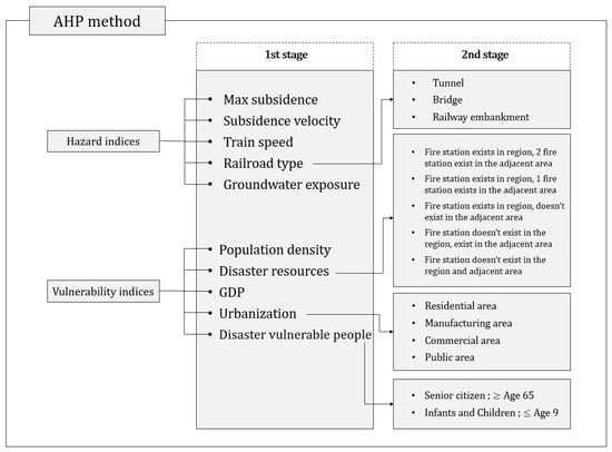
Figure 5.
Two-stage AHP framework used for risk assessment. The first stage includes ten primary indicators categorized into hazard and vulnerability indices. The second stage addresses three qualitative indicators—railroad type, urbanization, and disaster resource access—through subhierarchical evaluation to ensure consistent weighting.
However, three indicators, namely railroad type, urbanization, and disaster resource access, involve categorical or qualitative attributes that could not be fully evaluated using the standard 10-point AHP scale. To address this limitation, a second-stage AHP analysis was implemented, focusing on subcategories, such as the following: tunnel, bridge, and embankment for railroad type; residential, commercial, and public zones for urbanization; and five levels of fire station availability for disaster response capability.
This two-tiered approach allowed for the structured and consistent incorporation of both quantitative and qualitative factors, thereby enhancing the accuracy and interpretability of the final risk assessment model.
To determine the ten key indicators used for hazard and vulnerability assessment, the study relied on expert consultation with five faculty members specializing in civil engineering and disaster risk management, alongside considerations of spatial data availability. These indicators were selected to ensure both conceptual relevance and empirical feasibility within a geospatial risk assessment context. Following the selection, relative weights for each indicator were derived through a structured analytic hierarchy process (AHP) survey involving 25 participants. The expert panel included 20 graduate students from the Disaster & Risk Management Laboratory at Sungkyunkwan University (SKKU) and five faculty members—Professors Hongsik Yoon, Seunghee Park, and Am Jang from SKKU; Professor Jaejoon Lee from Chonnam National University; and Professor Moonsu Song from Kyungwoon University—all of whom possess substantial expertise in infrastructure safety and disaster risk analysis. To ensure the reliability of the survey results, any response with a consistency ratio (CR) exceeding 0.1 was excluded from the final analysis.
As summarized in Table 3, the results of the AHP analysis revealed that the highest-weighted hazard indicator was subsidence velocity (0.318), followed by groundwater discharge (0.245) and maximum subsidence (0.207). For vulnerability indicators, population density (0.247) and the urbanization rate (0.232) received the highest priority, while GDP ranked the lowest (0.146). These results reflect expert perceptions of the relative significance of each factor in assessing rail infrastructure risk.
Table 3.
Final pairwise comparison matrix with calculated weights and rankings for hazard and vulnerability indicators used in this study.
However, since some of the indicators, namely railroad type, urbanization, and emergency facility access, feature categorical or qualitative characteristics that are not easily captured using conventional AHP scaling, a second-stage hierarchical AHP analysis was performed. The results, presented in Table 4, provide refined weights for each subcategory, such as bridge sections (0.534) in railroad types and manufacturing areas (0.301) in building types. Notably, for emergency response capability, regions lacking both in-zone and adjacent fire stations were considered the most vulnerable, receiving the highest weight (0.313).
Table 4.
Refined subcategory weights derived from second-stage hierarchical AHP analysis for selected qualitative indicators.
This two-tiered approach was adopted to overcome the limitations of traditional AHP applications, which often rely on single-stage expert scoring and may lack sufficient granularity or objectivity in handling qualitative variables. By supplementing the primary indicator weighting with a secondary decomposition, this study enhances both the validity and the interpretability of the risk model.
2.3.2. Composite Risk Index Calculation
To enhance the validity of the AHP-derived weights and address the issue of potential redundancy among interrelated factors, this study employed a supplementary procedure to account for dependencies across indicators. While the analytic hierarchy process (AHP) enables a structured derivation of weights and consistency verification based on expert surveys, it inherently assumes mutual independence among evaluation criteria. However, as prior studies have highlighted, overlooking interdependencies among factors may result in overrepresentation or distorted weights, particularly in urban or infrastructure systems where indicator correlations are common [70,71,72,73].
To mitigate this issue, a dependency-adjusted weighting process was introduced by analyzing inter-factor correlations. Specifically, Euclidean distance was employed as a dissimilarity metric to capture the similarity between indicator pairs [74,75]. This approach draws on the methodological foundation proposed by [73], who emphasized that high correlation among decision factors can significantly distort AHP-based rankings, and recommended supplemental correction procedures. In parallel, the use of Euclidean distance aligns with the k-nearest neighbor (KNN)-based similarity computation method described by [76], which has been widely adopted in geospatial and environmental risk modeling.
In this study, the calculated Euclidean distances serve as the basis for a triangular distance matrix, representing the degree of dissimilarity among all indicator pairs. Each factor’s final dependency-adjusted weight was computed as the normalized inverse of its total Euclidean distances from other indicators—an approach shown to improve weight reliability and reduce bias in MCDM contexts [77,78].
By applying this formula to all factor pairs, a triangular distance matrix is constructed, as presented in Equation (3):
In this matrix, each element u(i,j) represents the Euclidean distance between factors i and j. The diagonal elements, which indicate zero distance (that is, the factor compared with itself), are excluded from the dependency weighting process.
The dependency weight of each factor is then determined by computing the normalized inverse of the sum of its Euclidean distances from all other factors. In this way, factors that exhibit greater similarity to others, reflected by lower cumulative distances, are assigned proportionally higher weights. This normalization ensures that highly correlated indicators do not exert excessive influence on the final risk index, thereby enhancing the robustness and balance of the assessment.
The results of this dependency-weighted analysis are visualized in Figure 6. By refining the AHP-derived weights with this adjustment procedure, the proposed risk model achieves greater accuracy and reduces the risk of multicollinearity in subsequent GIS-based risk mapping.
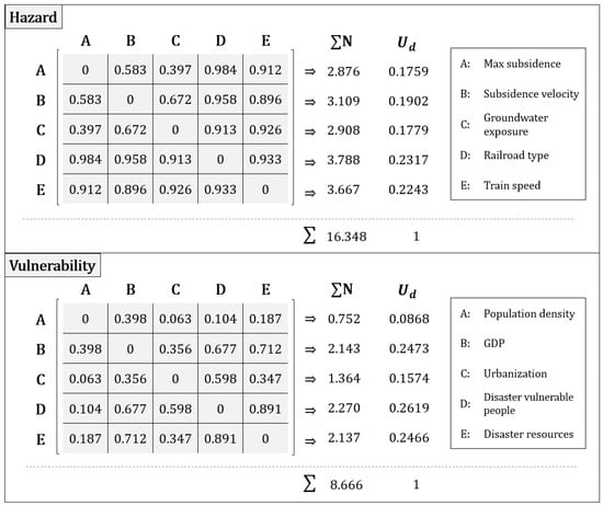
Figure 6.
Euclidean distance-based dependency weights for hazard and vulnerability indicators. The matrices display the pairwise Euclidean distances among indicators, with normalized weights Ud derived from the inverse of total distances.
Furthermore, this methodology is consistent with best practices observed in transportation planning and smart city applications, where fuzzy AHP, distance-based aggregation, and dependency-aware modeling have proven effective in complex decision environments [78,79].
2.4. Vulnerability Curve Assessment
To evaluate community-level vulnerability in conjunction with geotechnical hazards, this study introduces a vulnerability curve model that quantitatively relates hazard intensity to expected damage. Vulnerability, broadly defined, encompasses physical, social, economic, and environmental conditions that increase a community’s susceptibility to adverse hazard impacts. These dimensions align with the typologies proposed in the literature—physical vulnerability captures the structural susceptibility of buildings and infrastructure [80,81], economic vulnerability pertains to losses from business interruptions or economic exposure, social vulnerability refers to the risks faced by marginalized populations, and environmental vulnerability encompasses degradation from hazard interactions [82].
Ref. [82] further conceptualized vulnerability into two domains: external (exposure to hazard shocks and stressors such as earthquakes or resource depletion) and internal (coping ability or resilience deficits). Vulnerability curves have thus become a standard analytical tool to express these conditions in quantitative risk modeling. Rather than relying solely on hazard intensity, these curves enable modeling of how identical hazard events produce differential outcomes depending on community fragility [83].
Empirical and regression-based vulnerability functions have been applied across geotechnical domains, including mining subsidence [80], differential settlements [81], and landslide risk [84,85]. Particularly for debris flow and fluvial hazards, researchers such as [86,87] derived continuous damage functions using logistic or hyperbolic regression models. These parametric functions—often resembling fragility curves—allow for probabilistic damage estimation across intensity levels. Later works have refined these models for structure-specific applications such as rockfall-induced building collapse [88] or slow-moving landslides [83], with several adopting advanced formulations like the Avrami function [89].
In the present study, a vulnerability assessment was implemented as a foundational step for community-scale risk mapping along the Honam High-Speed Rail corridor. The primary hazard of interest was long-term subsidence triggered by geotechnical processes, with damage scenarios differentiated based on rail segment type (gravel vs. concrete). Maintenance and repair standards (Table 5) were used to establish damage thresholds for each segment type.
Table 5.
Damage classification and maintenance thresholds for gravel and concrete railway tracks based on subsidence levels.
For instance, ref. [90] evaluated the cumulative settlement behavior of railway embankments constructed using tunnel spoil and reported that routine settlement levels requiring maintenance typically range between 10 and 20 mm, which supports the thresholds defined for “normal repair” (10 mm for gravel and 7 mm for concrete) and “priority repair” (14 mm for gravel, 10 mm for concrete) in Table 5. Likewise, Ref. [91] reviewed international subgrade performance guidelines for high-speed railways and recommended maintaining cumulative subsidence below 15 mm to prevent deterioration of track geometry. This guidance is reflected in the “urgent repair” thresholds (18 mm for gravel and 14 mm for concrete), while the upper bounds for “allowable subsidence” (30 mm) and “failure” (50 mm) correspond to levels that may compromise structural safety if exceeded. These empirical and guideline-based findings provide validation for the tiered damage classification and maintenance actions summarized in Table 5.
Using these thresholds, vulnerability tables were generated separately for gravel (Table 6) and concrete tracks (Table 7), mapping subsidence intensity levels (in mm) to discrete damage grades (D0–D5). From these tables, expected damage values (Ed) were computed using the weighted average formula:
Table 6.
Ground settlement-based damage grades (D0–D5) for gravel tracks.
Table 7.
Ground settlement-based damage grades (D0–D5) for concrete tracks.
Subsequently, vulnerability curves were derived by regressing damage levels against subsidence intensity using the hyperbolic tangent formulation introduced by Saeidi et al. (2009) [80]:
This functional form enables the modeling of damage escalation as a function of incremental deformation, producing S-shaped curves that capture both the onset and saturation of damage. Curve fitting was conducted for each rail type to reflect infrastructure-specific vulnerability characteristics. The fitted results are presented in Figure 7, where the vulnerability curves for both gravel and concrete tracks clearly illustrate their respective deformation damage relationships.
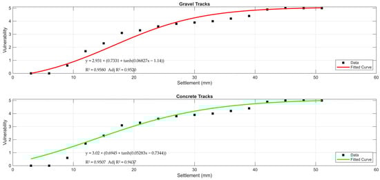
Figure 7.
Continuous vulnerability curves derived using hyperbolic tangent regression (Saeidi et al., 2009 [80]) underground settlement: red curve (gravel track, R2 = 0.9580), green curve (concrete track, R2 = 0.9507), and black squares (observed damage values).
Similarly, ref. [92] applied S-shaped fragility curves to assess subsidence-induced risks to transmission towers in a salt lake region, effectively characterizing nonlinear structural responses to ground deformation. Building on this approach, the present study extends its application to high-speed rail infrastructure, providing a quantitative basis for integrating vulnerability into the GIS-based risk mapping framework described in Section 2.5.
Building on this formulation, continuous vulnerability curves were developed separately for gravel and concrete tracks to reflect their differing structural responses to ground deformation. The fitted models revealed that the concrete track exhibits a slightly lower asymptotic vulnerability (~5.01) and a gentler slope (c = 0.05283) compared to the gravel track (~5.09, c = 0.06827). In terms of regression performance, the gravel track model achieved R2 = 0.9580 and adjusted R2 = 0.9520, while the concrete track model yielded R2 = 0.9507 and adjusted R2 = 0.9437. This difference also reflects the greater stiffness and structural continuity of concrete track systems, which tend to distribute deformation more evenly than gravel tracks.
These results indicate that concrete tracks experience a more gradual increase in damage under subsidence, ultimately reaching saturation in a smoother and more stable manner. This behavioral pattern has also been confirmed in recent machine learning-based infrastructure studies that modeled subsidence-induced ground instability using ensemble methods and artificial neural networks [93,94]. These studies demonstrated that data-driven vulnerability curves—linking settlement to structural performance—can be significantly flattened when predictive analytics are employed, allowing for the early detection and targeted reinforcement of vulnerable segments. As such, the vulnerability curve for concrete infrastructure may be regarded as more desirable, reflecting enhanced resilience and lower sensitivity to ground settlement compared to gravel tracks.
Notably, the Honam High-Speed Rail predominantly adopts concrete track structures, except for limited gravel track segments shared with conventional trains. This design choice aligns with the findings of [95], who emphasized that incorporating proactive mitigation and recovery measures into infrastructure design can reduce the steepness of damage–impact curves and improve long-term operational resilience. Accordingly, the risk assessment in this study focuses on the concrete track vulnerability curve to ensure consistency with real-world infrastructure conditions and to reflect the relative structural advantage of slab tracks in terms of subsidence tolerance.
This contrast in behavior between concrete and gravel track systems was effectively captured through the hyperbolic tangent–based regression framework applied in this study. This methodological approach models the nonlinear escalation of damage as a function of subsidence intensity and aligns with international best practices in infrastructure vulnerability modeling. It also complements recent advancements in resilience-focused urban infrastructure analytics, thereby reinforcing the broader relevance and applicability of the adopted risk analysis framework.
2.5. GIS-Based Risk Mapping
To effectively visualize and communicate the spatial distribution of risk along the Honam High-Speed Railway corridor, this study adopted a GIS-based risk mapping framework that integrates both PS-InSAR-derived hazard indicators and AHP-based vulnerability assessments. Geographic information systems (GISs) offer a robust platform for multi-criteria spatial analysis and have been extensively used in infrastructure risk studies due to their capacity to layer and synthesize diverse geospatial data [96,97,98,99,100].
The composite risk index, constructed through a weighted overlay of hazard and vulnerability layers, was spatially represented using raster-based risk zoning. Each input indicator was normalized and classified into ten intervals to ensure comparability across scales. Hazard indicators, such as subsidence magnitude, subsidence velocity, groundwater outflow, track type, and operational speed, were spatially derived from PS-InSAR analysis and operational data. Vulnerability indicators, including population density, GDP, the urbanization ratio, the proportion of vulnerable groups, and emergency facility accessibility, were also spatialized and classified.
To capture the broader impact zones beyond the rail line, kernel density estimation (KDE) was applied to model risk dispersion in a 1 km buffer area surrounding the rail corridor. This method, supported by prior infrastructure risk literature [101], allowed the visualization of secondary impact areas where the risk may extend into residential and urban zones.
The final output, shown in Figure 8, displays the risk landscape across the study region, highlighting zones categorized from “Very Low” to “Very High” based on composite scores.
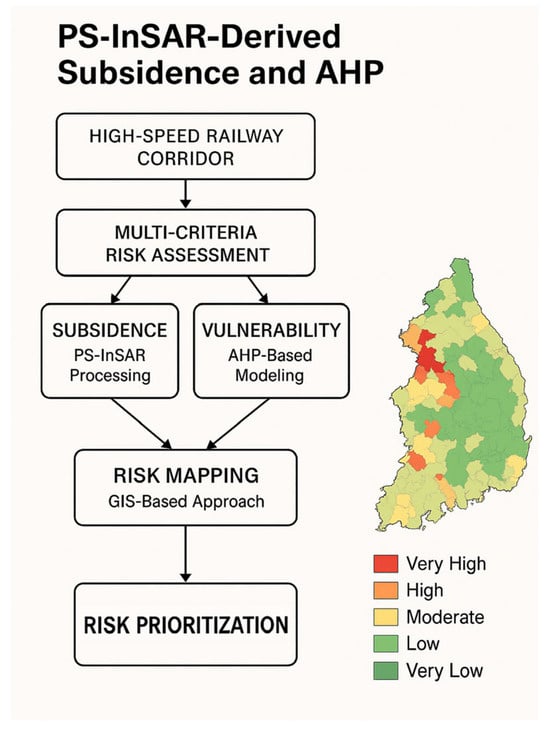
Figure 8.
Workflow for subsidence risk assessment along a high-speed railway corridor using PS-InSAR-derived deformation data and AHP-based vulnerability modeling. Subsidence and vulnerability layers are integrated using Euclidean distance for GIS-based risk mapping and subsequent risk prioritization. The resulting risk map classifies areas into five levels: very high, high, moderate, low, and very low. Risk levels are illustrative and intended as an example for methodological demonstration.
3. Results
This section presents the results of the risk assessment conducted for both high-speed railway infrastructure and the surrounding communities. The conceptual basis of this study follows the UN-ISDR definition of risk as the probability of loss, resulting from the interaction between hazards and vulnerabilities. This relationship can be mathematically expressed as follows:
In this context, vulnerability is defined as the set of physical, social, economic, and environmental conditions that increase a community’s sensitivity to the impacts of hazards. It can be categorized into four types: physical, economic, social, and environmental vulnerability.
To evaluate risk, this study adopts a two-tiered approach:
- Railway risk assessment, focused on the potential hazard posed by ground subsidence along the Honam High-Speed Railway line;
- Community risk assessment, based on a 0.5 km, 1 km, 2 km buffer around the railway line, reflecting areas potentially affected by accidents.
For this purpose, five hazard indicators were selected:
- Maximum ground subsidence;
- Subsidence velocity;
- Groundwater outflow;
- Railway structure type (tunnel, bridge, or embarkment);
- Sectional speed.
In parallel, five vulnerability indicators were defined:
- Population density;
- Local GDP;
- Urbanization rate;
- Proportion of vulnerable groups (children and the elderly);
- Presence of emergency and relief facilities.
Given the differing units and scales of the selected indicators, direct comparison was not feasible. To address this challenge, the analytic hierarchy process (AHP) was employed to derive relative importance weights for each indicator. In addition, to mitigate the effects of multicollinearity and inter-variable correlation, dependency weights were calculated using a Euclidean distance-based k-nearest neighbors (k-NN) similarity model.
Accordingly, the hazard and vulnerability components were first weighted using the dependency-based model, as shown in Equation (8):
To derive the final composite weights, this study averaged the AHP-derived weights and the dependency-based weights. The final weighted hazard and vulnerability expressions are provided in Equation (8):
The final composite weights for each indicator were obtained by averaging the AHP and dependency weights, forming a unified hazard and vulnerability index. These were then classified into ten levels to produce the final integrated risk map, which forms the basis for scenario-based risk analysis across the study area.
3.1. Railway Hazard Assessment
To assess community-level risk, this study builds upon existing railway hazard assessment frameworks by identifying and analyzing five key indicators that represent physical risk factors along the high-speed railway corridor.
Maximum ground subsidence was derived from PS-InSAR time-series data, capturing the largest vertical displacement observed during the monitoring period.
Subsidence velocity was calculated by tracking the displacement of corner reflectors at 17 locations at two-month intervals, enabling high-precision estimation of ground deformation rates. These values were then spatially interpolated across the Honam High-Speed Railway using inverse distance weighting (IDW), reflecting the intensity and urgency of ground movement over time.
Groundwater outflow was evaluated using national groundwater datasets from 2019 by analyzing changes in groundwater levels near the same 17 corner reflectors. The maximum annual fluctuation in groundwater level was selected as the hazard indicator and interpolated using IDW to represent subsurface hydrological instability affecting soil integrity.
Railway structure type was categorized into tunnels, bridges, and embankments. A total of 63 bridges and 34 tunnels along the Honam High-Speed Railway were surveyed, and the resulting structural data were interpolated using IDW. Vulnerability-based weights were then assigned according to the characteristics of each structure type.
Segmental train speed was estimated by analyzing departure and arrival times at each station, applying a range between 150 km/h and 310 km/h, to reflect actual travel speeds across different segments of the line. This indicator was used to assess the potential severity of accidents associated with high-speed operation.
3.1.1. Ground Subsidence Analysis
Ground subsidence was analyzed using time-series data obtained through the persistent scatterer interferometric synthetic aperture radar (PS-InSAR) technique. The maximum subsidence value was defined as the most negative displacement recorded during the observation period. This metric represents the peak vertical deformation affecting the railway alignment and serves as a critical indicator of physical hazard potential.
While maximum subsidence provides insight into the severity of ground settlement over time, it does not convey information about the rate or abruptness of the deformation process. As highlighted by Lee (2025) [24], such limitations necessitate the inclusion of supplementary indicators—such as subsidence velocity—for a more comprehensive risk assessment of high-speed rail systems.
Figure 9 illustrates the spatial distribution of normalized ground subsidence levels along the Honam High-Speed Railway corridor, as derived from PS-InSAR analysis. Subsidence values were classified into ten intervals, ranging from 1.56 mm to 46.47 mm, to visualize the severity and spatial variation of ground deformation. The color gradient from blue to red represents increasing levels of subsidence intensity. A 0.5 km and 1 km buffer zone around the railway line is also shown to indicate the potential area of impact for community risk assessment.
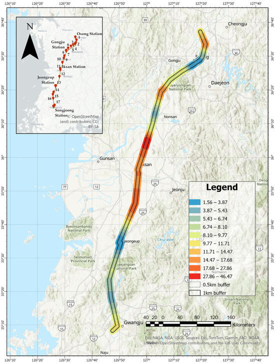
Figure 9.
Spatial distribution of normalized ground subsidence levels derived from PS-InSAR analysis along the railway corridor between Osong and Gwangju. Displacement values were normalized and classified into ten severity levels, with Level 1 indicating the lowest and Level 10 the highest subsidence. The color gradient represents increasing subsidence intensity in millimeters (mm), as shown in the legend. A 2 km buffer zone was applied around the railway to delineate the analysis area. The solid black lines represent a 1 km buffer, while the dashed lines indicate a 0.5 km buffer. The inset map in the upper left shows the locations of 17 corner reflector (CR) installations, along with major station names and the segment numbering used in the analysis.
Figure 9 illustrates the spatial distribution of ground subsidence along the Honam High-Speed Railway corridor, as estimated using the PS-InSAR technique. The analysis was based on a time series of 24 TerraSAR-X and 5 TanDEM-X SAR images acquired between August 2016 and September 2018. Following standard PS-InSAR processing steps—including coregistration, interferogram generation, atmospheric phase screen (APS) correction, and persistent scatterer identification—the displacement measurements were normalized and classified into ten subsidence levels.
The results reveal marked spatial heterogeneity in deformation severity across the corridor. Notably, segments near Iksan and northern Jeongeup exhibit the highest subsidence levels, reaching up to approximately 46 mm. The classification facilitates intuitive interpretation of risk-prone areas, with warmer colors (red to orange) indicating a higher subsidence intensity. The buffer zones (0.5 km: dashed line; 1 km: solid line) further contextualize the spatial extent of deformation relative to the railway alignment. These findings provide a basis for prioritizing maintenance and monitoring in geotechnically sensitive sections of the railway infrastructure.
3.1.2. Subsidence Velocity Evaluation
Subsidence velocity serves as a key indicator of the dynamic characteristics of ground deformation, quantifying the temporal rate of vertical displacement along the Honam High-Speed Railway (HSR) corridor. Unlike maximum subsidence, which captures only the total accumulated deformation, subsidence velocity incorporates the time dimension, providing critical insights into the abruptness and progression of settlement behavior.
In this study, high-precision subsidence velocity was estimated by tracking the displacement of corner reflectors at 17 selected locations at two-month intervals. This approach enabled the quantification of ground movement intensity and urgency over time. The derived velocity values were then spatially interpolated across the entire Honam HSR using inverse distance weighting (IDW), facilitating a continuous spatial representation of deformation dynamics along the corridor.
Velocity maps were generated by interpolating point-based subsidence velocity measurements into continuous spatial surfaces using inverse distance weighting (IDW). These maps were subsequently integrated into the risk model as a critical hazard layer. This approach enables the distinction between gradually evolving settlement patterns and abrupt subsidence events, thereby improving the spatiotemporal resolution of risk identification.
Areas with high subsidence velocity are typically associated with zones of significant geotechnical instability and infrastructure stress, particularly in sections where weak alluvial deposits underlie slab track systems. Incorporating velocity as a dynamic hazard indicator thus contributes to a more refined and responsive risk assessment framework, enhancing the effectiveness of infrastructure monitoring and early warning systems.
To validate the accuracy of the PS-InSAR-derived surface deformation measurements, a ground-based observation network was established along the Honam High-Speed Railway corridor. A total of 17 corner reflectors were strategically installed at selected sites spanning the entire railway alignment, as illustrated in Figure 10. These corner reflectors served as stable artificial targets to enhance radar signal returns and enable precise displacement tracking. Over a monitoring period of approximately two years, differential leveling surveys were conducted at two-month intervals, resulting in a total of 14 observation epochs. The high-precision leveling data obtained from these campaigns were used to detect subtle vertical ground movements at each reflector site. By comparing these field-derived displacements with the PS-InSAR measurements, the study assessed the consistency, reliability, and spatial accuracy of the satellite-based deformation estimates. This systematic validation approach suggests that the remote sensing data hold significant potential for application in subsidence risk mapping and infrastructure vulnerability analysis.
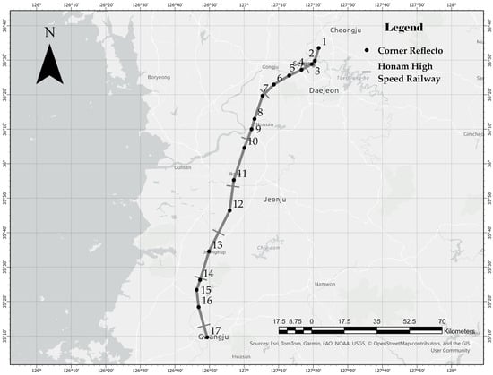
Figure 10.
Spatial distribution of 17 corner reflectors installed along the Honam High-Speed Railway corridor in South Korea for PS-InSAR validation. The corner reflectors (black dots) are positioned at regular intervals covering the entire railway alignment from Cheongju in the north to Gwangju in the south. The solid black line represents the railway route. These reflector sites served as stable ground control points for precise displacement monitoring through repeated leveling surveys. The data collected from these ground observations were used to assess the accuracy and reliability of PS-InSAR-derived ground deformation measurements. The basemap was generated using OpenStreetMap data and includes administrative boundaries and major cities for spatial reference.
To assess the accuracy of the PS-InSAR-derived ground deformation measurements, precise leveling surveys were conducted a total of 14 times at approximately two-month intervals. The resulting leveling data were compared with the corresponding PS-InSAR displacement values. Figure 11 presents the comparison between the PS-InSAR measurements and precise leveling data at Site 1, while the corresponding results for the remaining sites (Sites 2 through 17) are provided in Appendix A for reference.
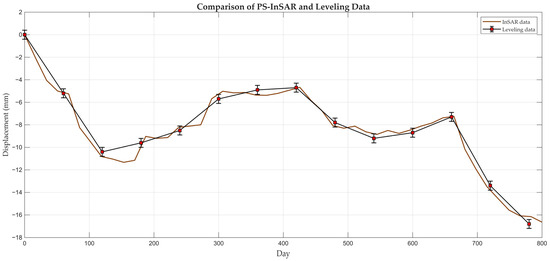
Figure 11.
Comparison of displacement between PS-InSAR data and leveling survey results for the first observation period. The red squares indicate the leveling measurements with associated error bars, and the brown line represents the PS-InSAR-derived displacement. The profile distance is shown on the horizontal axis, and the displacement in millimeters is shown on the vertical axis.
Figure 11 presents a comparative analysis between the first PS-InSAR-derived displacement measurements and corresponding precise leveling data at Site 1 during the initial monitoring period. The x-axis represents time in days, and the y-axis indicates vertical displacement in millimeters. Red markers denote leveling observations with associated error bars, while the blue line corresponds to the PS-InSAR measurements.
Figure 12 presents the root mean square error (RMSE) values between PS-InSAR-derived displacements and precise leveling measurements from 2016 to 2018 for each of the 17 reflector locations. The majority of RMSE values fall within the 2–3 mm range, indicating that the PS-InSAR technique provides displacement measurements with accuracy comparable to ground-based leveling. The full time-series comparisons for each reflector site are provided in Appendix B, Figure A9 and Figure A10.
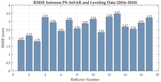
Figure 12.
Root mean square error (RMSE) between PS-InSAR-derived displacement and precise leveling data at 17 reflector sites along the study corridor (2016–2018). Most RMSE values range between 2 mm and 3 mm, demonstrating high consistency between satellite-based and ground-based measurements.
Figure 12 presents the spatial distribution of the annual ground subsidence rate along the Honam High-Speed Railway corridor, derived from PS-InSAR analysis. The estimated linear deformation rates were classified into ten levels based on magnitude (in mm/yr), enabling a clearer assessment of areas with relatively higher or lower subsidence velocity. The subsidence rates were interpolated using the inverse distance weighting (IDW) method, based on displacement measurements from 17 corner reflectors (CRs) installed along the corridor. The locations of these CRs are indicated by red dots in the inset map on the upper left.
Figure 9 and Figure 12 depict the spatial distribution of maximum ground subsidence and annual subsidence velocity, respectively, along the Honam High-Speed Railway corridor. While both maps highlight areas of deformation, notable differences in their spatial patterns can be observed due to methodological distinctions in data derivation.
The maximum subsidence map (Figure 9) was generated based on the PS-InSAR time-series analysis of all persistent scatterer (PS) points, capturing the most extreme vertical displacement recorded during the monitoring period. This provides a comprehensive view of localized ground settlement intensity across the entire corridor.
In contrast, the subsidence velocity map (Figure 12) was derived by tracking displacements at 17 strategically installed corner reflector (CR) sites, with measurements taken at two-month intervals. These point-based estimates were then converted into annual rates and spatially interpolated using IDW. As a result, the velocity map reflects generalized deformation trends, potentially smoothing localized anomalies but offering clearer insights into the temporal progression of settlement.
The variation between the two maps underscores the importance of integrating both static (maximum displacement) and dynamic (velocity) indicators to obtain a more holistic understanding of geotechnical risks affecting high-speed rail infrastructure.
Figure 13 illustrates the spatial distribution of annual ground subsidence rates along the Honam High-Speed Railway corridor, derived from PS-InSAR analysis. Subsidence velocities were calculated by tracking displacement at 17 corner reflector (CR) sites at two-month intervals, converted to annual rates (mm/year), and spatially interpolated using the inverse distance weighting (IDW) method.
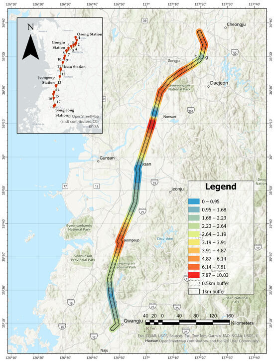
Figure 13.
Spatial distribution of annual ground subsidence rates (mm/yr) along the Honam High-Speed Railway corridor, derived from PS-InSAR analysis. The deformation velocities were interpolated using the inverse distance weighting (IDW) method based on displacement measurements from 17 corner reflectors (CRs). The subsidence rates were classified into ten levels, with warmer colors indicating higher annual settlement. A 2 km buffer zone was applied around the railway to define the analysis area. Solid black lines represent a 1 km buffer, while dashed lines indicate a 0.5 km buffer. The inset map in the upper left shows the locations of the 17 CR installations used in the interpolation.
The resulting velocity values were classified into ten levels, allowing for a clear distinction between areas with relatively low and high subsidence activity. The color gradient—ranging from blue (low velocity) to red (high velocity)—enables an intuitive visual identification of zones with potentially elevated geotechnical risk.
As shown on the map, segments between Iksan and Jeongeup, as well as parts of the Nonsan area, exhibit relatively high subsidence velocities, potentially associated with localized geotechnical factors such as heterogeneous subsoil conditions or groundwater fluctuations. In contrast, regions near Gwangju and Gongju display lower rates of vertical displacement, indicating relatively stable ground conditions.
This spatial distribution of subsidence velocity, as a dynamic hazard indicator, offers valuable input for long-term infrastructure risk assessment and supports the development of targeted maintenance and mitigation strategies for high-speed rail systems.
3.1.3. Groundwater Outflow Analysis
Groundwater Outflow was evaluated as a significant hydrological factor contributing to long-term ground deformation along the Honam High-Speed Railway (HSR) corridor. Excessive fluctuations or sustained decreases in groundwater levels can accelerate soil consolidation and induce vertical displacement, particularly in clay-rich or loosely deposited alluvial strata.
To quantify this factor, groundwater level data were obtained from [102], which provides time-series records from observation wells across the country. Among these, 17 monitoring wells located in the closest proximity to the corresponding 17 corner reflector (CR) sites along the Honam High-Speed Railway were selected. Groundwater level fluctuations at these sites were tracked over the course of one year (2019) to estimate local hydrological dynamics.
The minimum and maximum groundwater levels observed during this period were used to calculate the annual fluctuation range for each site. These values are summarized in Table 8, and the resulting groundwater variation intensity was interpolated across the entire railway corridor using the inverse distance weighting (IDW) method to generate a continuous spatial representation.
Table 8.
Annual groundwater level fluctuations (ΔGWL) at 17 corner reflector sites in 2019 (unit: m). Monthly groundwater levels recorded at monitoring wells closest to each PS-InSAR corner reflector site. The final column (ΔGWL) indicates the annual fluctuation, calculated as the difference between the maximum and minimum groundwater levels observed during the year.
This study analyzed the relationship between groundwater fluctuations and ground deformation (subsidence rates) using groundwater level data from 17 monitoring sites provided in Table 8. The PS-InSAR data were collected from 2016 to 2018, while groundwater displacement measurements were conducted in 2019, making direct comparisons challenging. However, despite this temporal discrepancy, the study provided valuable insights into the relationship between groundwater level changes in 2019 and the ground deformation observed in the PS-InSAR data.
Seasonal variations in groundwater levels were observed, with the monsoon season (June–August) showing peak groundwater levels and the dry season (October–February) corresponding to decreases in groundwater levels, as evidenced by the data in Table 8. For instance, in CR ID 4, groundwater levels increased between June and August, while a decrease was noted from October to February. Similar patterns of groundwater increase during the summer and decrease during the dry season were observed in CR IDs 5, 7, 9, and 10.
The analysis of the impact of these seasonal changes on subsidence rates revealed a correlation between increased groundwater levels during the summer and reduced subsidence rates, and decreased groundwater levels during the dry season and increased subsidence rates. For example, in CR ID 9, groundwater levels increased from June to August, leading to a reduction in subsidence rates, while from October to February, subsidence rates showed an upward trend.
This analysis provides essential foundational data for understanding the temporal relationship between groundwater fluctuations and subsidence rates. Specifically, the increase in groundwater levels leads to soil expansion and ground stabilization, resulting in reduced subsidence rates, while a decrease in groundwater levels accelerates consolidation, leading to increased subsidence rates. This temporal analysis is crucial for further investigations into the effects of groundwater fluctuations on ground deformation, particularly in the context of infrastructure risk management.
Figure 14 illustrates the spatial distribution of maximum annual groundwater level variation along the Honam High-Speed Railway corridor. Based on the ΔGWL values recorded at 17 corner reflector sites (as presented in Table 8), the data were spatially interpolated using the inverse distance weighting (IDW) method. This approach facilitates the identification of hydrologically sensitive zones where substantial groundwater level fluctuations may contribute to subsurface instability and long-term deformation risks.
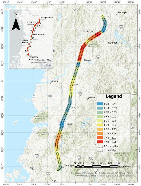
Figure 14.
Spatial distribution of annual groundwater level fluctuations (ΔGWL, in meters) along the Honam High-Speed Railway corridor. The map illustrates spatial variability in hydrological dynamics by classifying groundwater level changes into ten categories. Higher ΔGWL values—particularly in the northern (Osong) and southern (Gwangju) sections—indicate areas with more pronounced seasonal or anthropogenic influences on aquifer systems. The interpolation was performed using the inverse distance weighting (IDW) method based on monthly groundwater data from wells closest to each of the 17 corner reflectors (CRs). CR locations are marked as red dots in the inset map. A 2 km corridor buffer was applied, with solid black lines denoting the 1 km buffer and dashed lines indicating the 0.5 km buffer zones.
Figure 14 reveals the spatial heterogeneity of groundwater level fluctuations (ΔGWL) along the Honam High-Speed Railway corridor. Notably, elevated ΔGWL values—exceeding 1.5 m—were observed in southern segments near Gwangju and northern zones around Osong, indicating regions with pronounced hydrological variability. In contrast, the central corridor exhibited relatively stable groundwater conditions with fluctuations below 0.7 m.
These spatial patterns align with known variations in hydrogeological settings, including the presence of shallow unconfined aquifers and differential pumping intensities. Areas with large ΔGWL values correspond to locations where seasonal recharge–discharge cycles or excessive groundwater withdrawal may trigger consolidation in compressible soil layers, thus amplifying the potential for vertical ground displacement.
The integration of this ΔGWL layer into the broader risk assessment framework allows for the identification of subsurface vulnerability hotspots. As groundwater-induced settlement often evolves gradually yet persistently, such mapping is essential for early detection of latent geomechanical hazards that could compromise the structural integrity and long-term performance of high-speed rail infrastructure.
3.1.4. Railway Structure Type Classification
The type of track structure was considered a critical factor influencing ground deformation susceptibility along the Honam High-Speed Railway (HSR) corridor. As described in Section 2, the corridor was classified into three primary structural types: tunnels, bridges, and embankments. Each type exhibits distinct geotechnical behavior and varying sensitivity to subsurface movement.
Unlike other indicators in this study, which were normalized into ten levels using statistical methods, the railway structure factor was categorized into three levels based on weights derived from the analytic hierarchy process (AHP) during the criteria evaluation phase. Specifically, AHP-derived scores of 3.23, 5.34, and 1.43 were assigned to bridge, tunnel, and embankment sections, respectively.
Furthermore, using the extended AHP methodology presented in Table 4 of Section 2.3, structure-specific weights were assigned to 63 bridges and 34 tunnels along the Honam HSR. These weights were then spatially interpolated across the entire corridor using the inverse distance weighting (IDW) method, with the resulting distribution visualized in Figure 15. Table 9 summarizes the major overpasses and tunnels included in the analysis. A full list of all 90 structures and their corresponding tunnel sections is provided in Appendix A, Table A1.
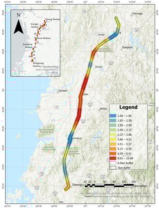
Figure 15.
Spatial distribution of structure-specific vulnerability scores along the Honam High-Speed Railway corridor. The map visualizes vulnerability levels by classifying interpolated AHP-based scores into ten categories. Higher values—particularly near Iksan and Jeongeup—indicate segments with greater structural vulnerability due to bridge and tunnel configurations. The interpolation was conducted using the inverse distance weighting (IDW) method based on structure-specific weights assigned to 63 bridges and 34 tunnels. A 2 km corridor buffer was applied; solid black lines represent the 1 km buffer, while dashed lines indicate the 0.5 km buffer zones. The red dots in the inset map denote major station locations and segment indices.
Table 9.
Overview of structure types, counts, and representative examples along the Honam HSR corridor.
Figure 15 presents the spatial distribution of structure-specific vulnerability scores along the Honam High-Speed Railway (HSR) corridor. As described in Section 2.3, the scores were derived using the extended analytic hierarchy process (AHP) methodology applied to 63 bridges and 34 tunnels, and spatially interpolated using the inverse distance weighting (IDW) method. The interpolated values were classified into ten levels to reflect spatial heterogeneity in vulnerability along the corridor.
The results show a concentration of high vulnerability scores in the central section of the corridor, particularly between Iksan and Jeongeup, where bridge and tunnel density is notably high. The accumulation of such structures contributes significantly to the overall structural risk, and it was incorporated as one of the key input layers in the total railway risk map developed in this study.
3.1.5. Train Speed Estimation by Segment
Segment speed is one of the operational factors that may influence the response characteristics of high-speed railway infrastructure to ground deformation. Trains operating at higher velocities could be more exposed to physical impacts when encountering subsidence or uneven ground conditions. Accordingly, quantifying and spatially representing segment-level train speeds can provide useful reference data for risk assessment.
Due to the unavailability of actual speed profiles from the Korea Railroad Corporation (KORAIL), a reverse estimation method was employed to compute representative segment speeds. The approach utilized publicly available information, including the scheduled travel time between stations, interstation distances, and the train’s maximum speed. Based on this information, the segment speed was derived using a trapezoidal velocity profile model that assumes linear acceleration and deceleration phases.
Figure 16 presents the conceptual velocity profile used in the speed estimation process. The total distance (Dtotal) was calculated using the area under the trapezoidal speed-time curve, and the time spent at maximum velocity (t) was estimated by subtracting acceleration/deceleration phases from the total travel time (T). This allowed the estimation of the acceleration/deceleration distance (d) for each interstation segment. The resulting equations, depicted in Figure 16, provided a consistent and logical framework for calculating segment-level speeds.
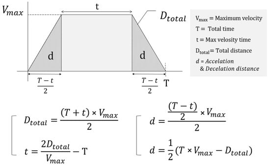
Figure 16.
Conceptual velocity profile and equations used to estimate segment speed based on trapezoidal motion between two stations.
Figure 17 shows the spatial distribution of estimated segment-level train speeds along the Honam High-Speed Railway corridor. Train speeds were classified into ten levels through normalization, allowing consistent integration with other hazard indicators in the AHP framework. Faster segments imply higher dynamic loads and shorter response times, increasing derailment risk in subsidence-prone areas. This normalized speed data contributes to the overall risk map by representing operational vulnerability related to train velocity.
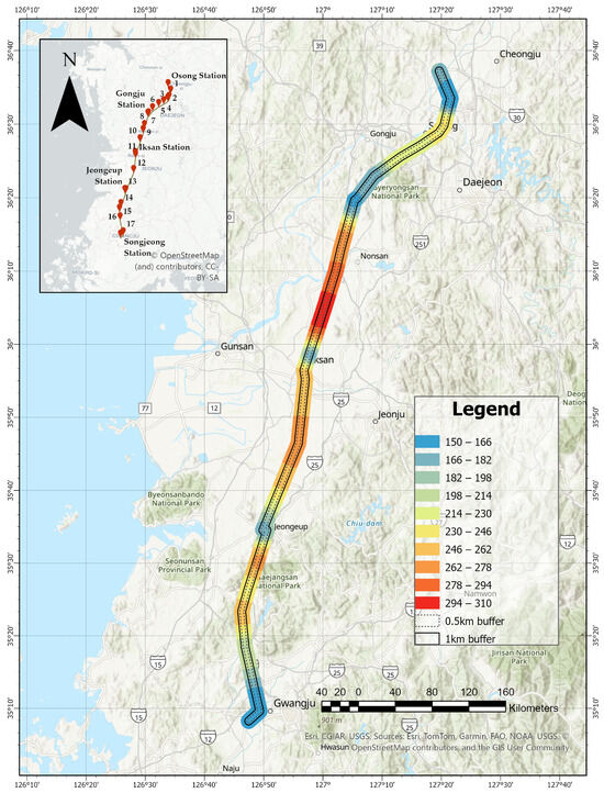
Figure 17.
Spatial distribution of estimated segment-level train speeds along the Honam High-Speed Railway corridor. The map visualizes calculated speeds, derived using a trapezoidal velocity profile model based on interstation distances and scheduled travel times, classified into ten categories. Due to the unavailability of actual speed profiles, the estimation was performed using publicly available data. A 2 km corridor buffer was applied; solid black lines represent the 1 km buffer, while dashed lines indicate the 0.5 km buffer zones. The red dots in the inset map indicate the locations of 17 corner reflectors (CRs) and all station stops along the corridor used in the analysis.
The spatial distribution of estimated train speeds shown in Figure 17 provides critical insight into segment-level vulnerability across the Honam High-Speed Railway (HSR) corridor. Segments with relatively higher speeds—particularly those in the central corridor near Iksan and Jeongeup—may present elevated risk levels in the event of ground deformation. In such segments, the reduced reaction time associated with high-speed operation increases the potential for damage when sudden subsidence or abrupt changes in ground conditions occur.
High-speed zones typically coincide with long, uninterrupted stretches where trains operate at or near their maximum velocity. In these areas, even minor structural displacements or geomechanical shifts may pose significant safety concerns due to the dynamic forces involved. Furthermore, bridge and tunnel concentrations within these zones can amplify vulnerability, as structural rigidity combined with high kinetic energy leaves little margin for error.
In contrast, terminal areas such as Osong and Gwangju, where speeds are generally lower due to deceleration and acceleration patterns, may be less exposed to sudden-impact risks but remain susceptible to cumulative stress effects over time.
Overall, the speed distribution map serves as a valuable indicator for identifying priority monitoring zones. The integration of speed data into the broader risk framework highlights its role as a critical weighting factor in segment-level vulnerability assessments.
3.1.6. Composite Physical Risk Index Mapping
To comprehensively assess the ground deformation risk along the Honam High-Speed Railway (HSR) corridor, five key contributing factors were selected: maximum subsidence, subsidence velocity, groundwater outflow, track structure type, and segment speed. These indicators inherently differ in unit, scale, and physical meaning, requiring a standardized framework to enable integrated comparison and modeling.
Accordingly, each indicator was normalized into ten ordinal levels using the natural breaks classification method. An analytic hierarchy process (AHP) was conducted to derive priority weights for each indicator, which were then combined with their respective dependency coefficients to generate a weighted linear combination. The result was an integrated risk index representing the spatial likelihood of subsidence-induced hazard along the railway line.
Figure 18 illustrates the composite physical risk index map for the Honam High-Speed Railway corridor, developed through the integration of five spatial indicators: (1) maximum ground subsidence, (2) subsidence velocity, (3) groundwater outflow, (4) railway structure type, and (5) train speed. Due to the differences in units, scales, and physical interpretations across these indicators, each dataset was spatially mapped and normalized into ten ordinal classes using the natural breaks classification method.
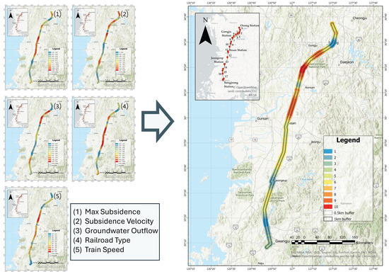
Figure 18.
Composite physical risk index map for the Honam High-Speed Railway corridor, derived from the integration of five spatial indicators: maximum subsidence, subsidence velocity, groundwater outflow, railway structure type, and train speed. Each indicator was normalized into ten ordinal levels using the natural breaks classification method. The final index was computed using a weighted linear combination based on AHP-derived priority weights. Spatial buffers of 0.5 km and 1 km from the railway centerline were applied to define the analysis extent. This index is intended to be combined with the vulnerability map as part of the final outcome in the spatiotemporal risk modeling of high-speed rail infrastructure.
To quantify the relative importance of each factor, the analytic hierarchy process (AHP) was employed based on the pairwise comparison results presented in Section 2.3.2 and Figure 6. This analysis yielded the following priority weights: 0.293 for maximum subsidence, 0.196 for subsidence velocity, 0.151 for groundwater outflow, 0.213 for railway structure type, and 0.147 for train speed. To further refine the weighting scheme and account for potential redundancies among the indicators, these AHP-derived weights were adjusted using dependency coefficients calculated from a Euclidean distance-based similarity matrix.
The final composite risk index was computed using a weighted linear combination of the normalized indicator layers. This index provides a spatially explicit representation of the hazard potential induced via ground deformation along the railway alignment. It serves as a key output of the hazard-based assessment and offers a valuable basis for risk-informed decision-making in future infrastructure management and planning. Furthermore, the index is integrated with the composite vulnerability map to constitute the final outcome of a comprehensive analytical framework for spatiotemporal risk modeling of high-speed rail infrastructure using PS-InSAR and AHP.
Figure 19 presents a zoom-in analysis of a high-risk section near Gongju Station along the Honam High-Speed Railway corridor. This area was identified as the segment with the highest composite hazard risk, where multiple risk factors converge. Within a 2 km buffer zone from the railway centerline, a concentrated distribution of elevated risk levels is clearly visualized. The inset map highlights spatial transitions in hazard intensity, suggesting that the combined effects of ground subsidence, groundwater outflow, structural configuration, and train speed significantly increase the vulnerability of this segment. Such localized analysis provides critical insight for site-specific risk mitigation planning and targeted infrastructure reinforcement strategies.
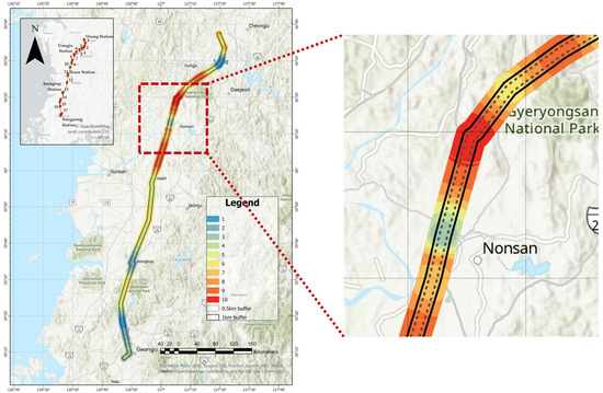
Figure 19.
Localized zoom-in analysis of a high-risk segment near Gongju Station along the Honam High-Speed Railway corridor. This section was identified as having the highest composite hazard risk. The inset highlights a concentrated distribution of high-risk values within spatial buffers of 0.5 km and 1 km from the railway centerline, delineated by dashed and solid lines, respectively. The spatial transitions in hazard levels suggest the combined influence of multiple contributing factors, including ground subsidence, subsidence velocity, groundwater outflow, railway structure type, and train speed. This detailed visualization provides critical input for targeted site-specific risk mitigation strategies and infrastructure planning.
3.2. Community Vulnerability Assessment
While infrastructure-centric hazard evaluation provides insight into the physical risk associated with rail-induced ground deformation, a comprehensive disaster preparedness framework must also consider the vulnerability of surrounding communities. Community vulnerability refers to the degree to which a population is exposed to and unable to cope with the impacts of a disruptive event. In this context, it serves as a metric for estimating the potential social damage resulting from a railway-related hazard, such as track subsidence or derailment.
This study assessed community vulnerability based on a combination of demographic, urban, and institutional indicators. Areas with higher population density, greater proportions of mobile or transient populations, and higher rates of urbanization are generally more susceptible to severe consequences due to greater exposure and concentration of assets. Conversely, the presence of emergency response facilities, such as fire stations, general hospitals, and police stations, contributes to increased coping capacity and thereby reduces overall vulnerability.
By quantifying and spatially mapping these factors, a vulnerability index was generated for the regions surrounding the Honam HSR corridor. This enables the identification of critical zones where a combination of high hazard potential and weak response infrastructure may amplify disaster risk. The results from this analysis are integrated with the hazard intensity map to derive a comprehensive rail-related disaster risk assessment, supporting both preventive planning and emergency response strategy development.
3.2.1. Population Density Mapping
Population density is a key demographic factor in assessing vulnerability, particularly in infrastructure risk analysis. Areas with a higher population density are more likely to experience greater social and economic impacts in the event of infrastructure failure, including potential hazards associated with high-speed rail (HSR) operations. In this study, population density data were obtained from the Korean Statistical Information Service [103], based on the most recent administrative-level dataset as of February 2019. The data were provided at the eup, myeon, and dong levels—the smallest administrative divisions in South Korea—allowing for high spatial resolution and detailed vulnerability analysis along the Honam High-Speed Railway (HSR) corridor. Additionally, the population density of each administrative unit (expressed as persons per km2) is presented in Appendix B, Table A6, serving as a reference for comparative vulnerability assessment and spatial interpretation across the study region.
The population figures were normalized to density values (persons/km2) and then converted into a GIS-compatible format for spatial analysis. The data were subsequently spatially joined with the administrative boundaries intersecting the Honam HSR impact zone. To categorize the population density data, a natural breaks classification method was applied, dividing the range of densities into ten distinct risk levels. The observed population density values ranged from 26 to 15,603 persons/km2, with the densest urban neighborhoods, such as parts of Gwangju and Iksan, falling into the highest categories.
Figure 20 presents the spatial distribution of population density along the Honam High-Speed Railway (HSR) corridor. The population data, sourced from administrative units at the eup, myeon, and dong levels, were normalized to persons per square kilometer and processed in a GIS-compatible format. A natural breaks classification method was applied to divide the density values into ten ordinal classes, allowing for a high-resolution demographic assessment of the surrounding areas. This layer serves as a core indicator in the vulnerability analysis framework for evaluating community exposure to potential railway-related hazards.
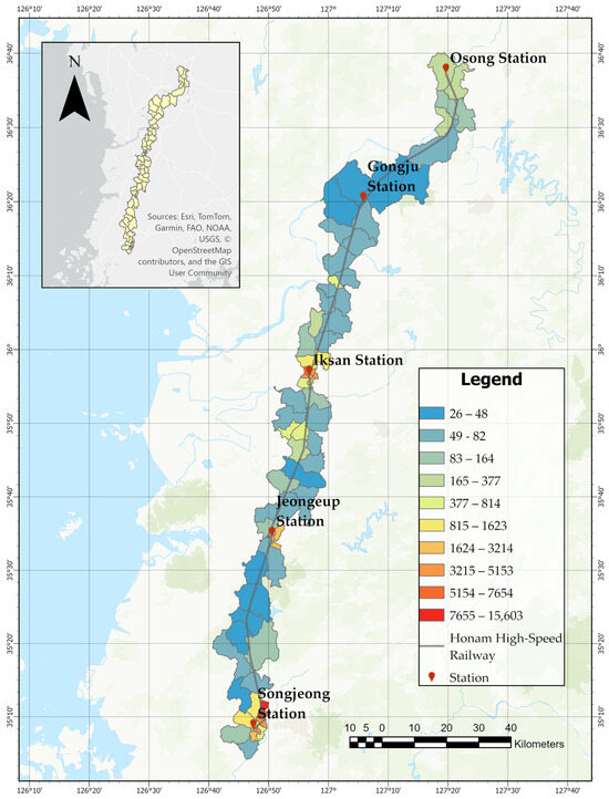
Figure 20.
Population density map of the administrative regions intersecting the Honam High-Speed Railway (HSR) corridor. The population data, based on eup, myeon, and dong administrative units as of February 2019, were sourced from the Korean Statistical Information Service (KOSIS) and spatially represented through GIS analysis. This map visualizes the residential concentration along the railway corridor and serves as a key indicator for assessing population exposure in railway-related hazard analysis. The inset map in the upper left shows the location of the administrative units included in the analysis.
As shown in Figure 20, population density varies markedly along the Honam High-Speed Railway (HSR) corridor, with notable concentrations not only near terminal urban centers but also within high-risk segments in the midline of the corridor. In particular, areas such as Iksan and Nonsan, while not classified as major metropolitan regions, exhibit moderate to high population densities due to their regional connectivity and patterns of urban development. These central segments, characterized by both operational railway infrastructure and residential clustering, may face elevated levels of exposure in the event of ground deformation or other rail-related hazards. The spatial concentration of population in these areas highlights the importance of incorporating midline regional characteristics into infrastructure risk management and emergency preparedness planning.
3.2.2. GDP-Based Economic Exposure Evaluation
The gross domestic product (GDP) represents the economic capacity of a region and is commonly used as a proxy for potential property damage in disaster risk assessments. Higher regional GDP values typically indicate greater concentrations of assets and infrastructure, suggesting elevated levels of economic loss in the event of a disruption. As such, GDP was adopted in this study as a socioeconomic indicator to evaluate the vulnerability of communities surrounding the Honam HSR corridor.
Regional GDP data were obtained from the Korean Statistical Information Service [103], the same source used for the population density analysis. While demographic data are available at finer administrative levels (eup, myeon, and dong), GDP figures are only published at broader administrative units (si, gun, and gu). As such, the analysis was conducted at a coarser spatial resolution, which may introduce some limitations in precision. Nevertheless, the data remain valuable for identifying regional economic exposure to potential hazards. The GDP values for each administrative unit are summarized in Appendix B, Table A6, and were spatially joined with the corresponding boundaries for integration into the vulnerability assessment.
Figure 21 illustrates the spatial distribution of gross regional domestic product (GRDP) in areas surrounding the Honam High-Speed Railway (HSR) corridor. GRDP serves as a key socioeconomic indicator reflecting the economic capacity and asset concentration within a given region, and is widely used to estimate the potential scale of economic losses in the event of infrastructure-related disasters.
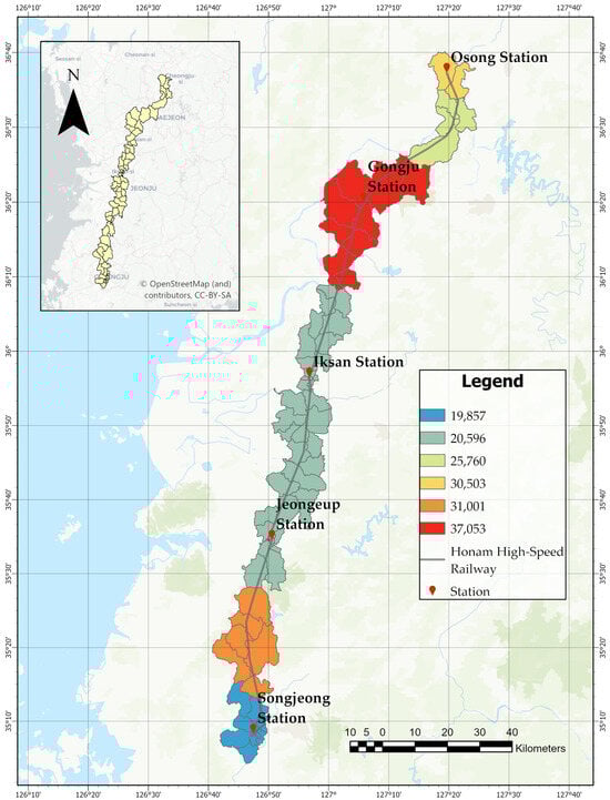
Figure 21.
Spatial distribution of gross regional domestic product (GRDP) along the Honam High-Speed Railway (HSR) corridor. This map displays GRDP values (in USD per year) aggregated at the si, gun, and gu administrative levels, which reflect the economic exposure of regions adjacent to the railway line. GRDP is used as a proxy for regional economic capacity and asset concentration, offering insights into the potential severity of financial losses in the event of infrastructure failure. Higher GRDP values, shown in red, are observed in major economic centers such as Gongju and parts of Osong, indicating heightened disaster vulnerability due to asset density. The inset map shows the full extent of administrative boundaries used for the assessment.
Figure 21 highlights notable spatial disparities in regional economic capacity along the Honam High-Speed Railway (HSR) corridor. The highest GRDP values are observed in Gongju and Osong areas, indicating a high concentration of economic assets and infrastructure. These economically intensive zones are potentially more vulnerable to substantial financial losses in the event of a rail-related disruption, such as ground deformation or service interruption.
In contrast, southern sections of the corridor, particularly around Gwangju and Jeongeup, exhibit lower GRDP levels, suggesting relatively reduced economic exposure. While these areas may face less direct economic loss, the presence of critical infrastructure still necessitates strategic risk management.
The variation in GRDP along the corridor emphasizes the importance of tailoring disaster mitigation strategies according to regional economic characteristics. Regions with both high GRDP and elevated physical hazard levels warrant prioritized investment in resilience measures to safeguard economic stability.
3.2.3. Urbanization Rate Analysis
The urbanization rate represents the extent of built-up development within a region, and it is a critical component of community vulnerability assessment. Areas with higher degrees of urbanization often have greater concentrations of infrastructure, assets, and populations, making them more susceptible to widespread damage in the event of a disaster. Moreover, highly urbanized environments tend to exhibit lower adaptive capacity due to impervious surfaces, limited evacuation routes, and increased exposure density.
In this study, urbanization data were acquired from the Environmental Geographic Information Service [104]. Building footprint layers were extracted and classified into four primary categories based on their functional use: industrial facilities, commercial facilities, residential buildings, and public institutions. These categories were evaluated using the analytic hierarchy process (AHP), and corresponding dependency weights were assigned to each subcategory to reflect their relative contribution to urban vulnerability.
For example, commercial and residential areas were given higher weights due to their population concentration, while public facilities were considered as lower impact zones. These weighting values correspond to the building type weights presented in Table 4, which reflect the relative contribution of each land use category to urban vulnerability based on population exposure and functional criticality. The weights were as follows: commercial area (0.232), industrial area (0.301), residential area (0.280), and public facilities (0.187). The proportion of each area type within the study region is provided in Appendix B Table A6.
Figure 22 illustrates the spatial distribution of the urbanization rate along the Honam High-Speed Railway corridor. The urbanization rate was calculated as the ratio of built-up area within each administrative unit and serves as a key indicator for assessing infrastructure concentration and urban vulnerability in the region.
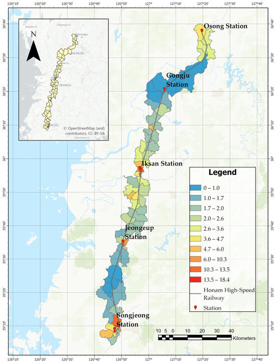
Figure 22.
Spatial distribution of the urbanization rate along the Honam High-Speed Railway corridor. The map visualizes the percentage of built-up area within each administrative boundary, derived from national building footprint datasets provided by the Environmental Geographic Information Service (EGIS). The urbanization rate was computed by calculating the ratio of built-up area to total land area within each unit, then classified into ten ordinal categories using the natural breaks method. Higher urbanization rates, represented in orange and red, indicate regions with greater infrastructure concentration and potentially higher vulnerability in the event of a disaster. Urban centers near Songjeong and Iksan Stations show the highest levels of urban development, suggesting increased exposure to infrastructure-related hazards.
Figure 22 presents the spatial distribution of the urbanization rate along the Honam High-Speed Railway (HSR) corridor. The urbanization rate, defined as the ratio of built-up area to total land area within each administrative unit, serves as a proxy for infrastructure and asset concentration. Regions with higher urbanization rates are generally more vulnerable to extensive damage in the event of a disaster, due to greater exposure and density of critical elements.
Using national building footprint data from the Environmental Geographic Information Service (EGIS), the urbanization rate was computed and categorized into ten ordinal classes through the natural breaks classification method. The results reveal that urban areas near Songjeong and Iksan Stations exhibit the highest urbanization rates, exceeding 13.5%, indicating strong alignment with dense residential and commercial activity. In contrast, rural segments around Jeongeup and Gongju Stations show significantly lower levels of urban development.
This spatial disparity underscores the need to account for varying levels of urban vulnerability in disaster preparedness and infrastructure resilience planning. The urbanization rate, as an indicator, provides essential spatial insight for developing targeted risk mitigation strategies.
3.2.4. Vulnerable Group Identification
The presence of disaster-vulnerable groups, particularly children and the elderly, significantly increases a community’s exposure in emergency scenarios due to reduced mobility and heightened need for assistance. These groups face increased difficulty evacuating during sudden events such as train derailments or infrastructure collapse, making them a critical component of vulnerability assessments.
In this study, vulnerable populations were defined using demographic data from the Korean Statistical Information Service (KOSIS; http://kosis.kr). Specifically, individuals aged 0–9 years were classified as children and those aged 65 years and older as elderly. The data were collected at the eup, myeon, and dong administrative levels, ensuring a fine spatial resolution across the study area.
Figure 23 presents the spatial distribution of vulnerable population ratios in the vicinity of the Honam High-Speed Railway corridor. The map depicts the proportion of disaster-sensitive groups, specifically individuals under the age of 9 and those aged 65 and older, normalized by the total population within each administrative unit. This demographic-based metric serves as a critical indicator for assessing community-level vulnerability and emergency preparedness capacity.
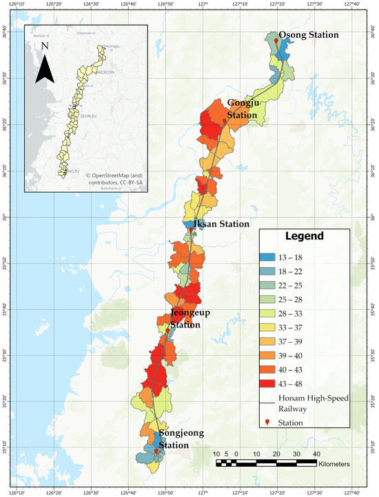
Figure 23.
Spatial distribution of disaster-vulnerable population ratios along the Honam High-Speed Railway corridor. Vulnerability is calculated as the proportion of children (under age 9) and elderly individuals (over age 65) relative to the total population in each administrative unit. Data were collected at the eup, myeon, and dong levels and classified into ten categories using the natural breaks method. Regions with higher ratios indicate greater potential difficulty in evacuation and response during hazard events. The inset map in the upper left corner shows the broader administrative boundary context of the study area.
Figure 23 presents the spatial distribution of disaster-vulnerable population ratios along the Honam High-Speed Railway (HSR) corridor. The vulnerability metric was derived from demographic data, specifically the proportion of individuals aged under 9 and over 65 within each administrative unit, as these groups are considered to have reduced mobility and heightened dependency in emergency scenarios.
The analysis reveals that several areas—including parts of Jeongeup, peripheral districts of Iksan, and southern sections of Gwangju and Jangseong—exhibit vulnerability ratios exceeding 40%. These zones may face substantial challenges in evacuation and emergency response operations during infrastructure failures, such as ground subsidence or derailments. Accordingly, they represent high-priority regions for preemptive disaster planning and targeted deployment of emergency services.
In contrast, regions near Sejong City and Osong Station show comparatively lower vulnerability ratios, falling below 20%. These areas, characterized by a younger population structure, may possess comparatively higher resilience in terms of community mobility and response capacity.
This demographic-based index offers valuable insights when interpreted in conjunction with other socioeconomic and physical indicators such as urbanization rate and GRDP. It enables the identification of spatial risk disparities and supports the formulation of tailored, region-specific disaster mitigation strategies for communities situated along critical high-speed rail infrastructure.
3.2.5. Emergency Facility Accessibility Assessment
The availability and spatial distribution of emergency relief facilities play a vital role in minimizing disaster impact through rapid response and coordinated rescue operations. In the event of railway-related accidents such as derailment or infrastructure failure, the proximity to fire stations and 119 rescue centers significantly influences the community’s capacity for immediate evacuation and medical support.
In this study, relief facility accessibility was evaluated through a five-level classification system based on both direct presence and spatial adjacency. The classification considered whether a given administrative unit contains a fire station and whether neighboring units also possess such facilities. This allowed for a more nuanced understanding of emergency infrastructure coverage, accounting for both local and regional response capabilities.
The five categories include the following: (1) regions with a fire station and two adjacent areas also covered; (2) those with a fire station and one adjacent covered area; (3) areas with a station but no adjacent support; (4) those without a fire station but with nearby coverage; and (5) regions with neither a fire station nor adjacent access. These classifications were assigned integer values and converted into a categorical vulnerability layer.
Figure 24 presents the spatial distribution of emergency facility accessibility along the Honam High-Speed Railway corridor. This map visualizes the results of a five-level classification scheme based on the presence of fire stations within each administrative unit and the coverage provided by adjacent areas.
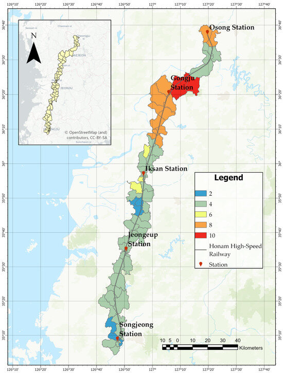
Figure 24.
Spatial representation of emergency facility accessibility along the Honam High-Speed Railway corridor. The map classifies each administrative region into five categories based on the presence of a fire station within the region and its surrounding areas: (1) regions with a fire station and two neighboring regions also covered, (2) regions with a fire station and one adjacent area covered, (3) regions with a fire station but no adjacent support, (4) regions without a fire station but with nearby coverage, and (5) regions lacking both internal and adjacent access to emergency facilities. These categories were converted into integer scores, creating a categorical vulnerability layer for use in subsequent integrated risk analysis. The inset map in the upper left shows the full extent of the study area’s administrative boundaries.
The classification highlights variations in emergency response infrastructure across the region, serving as a critical reference for evaluating community readiness and informing risk-based emergency planning in the event of railway-related disasters.
Figure 24 illustrates the spatial distribution of emergency response infrastructure accessibility along the Honam High-Speed Railway corridor. The classification scheme, based on both the presence of fire stations within administrative units and the availability of such facilities in adjacent areas, was used to categorize regions into five levels of emergency service coverage.
Notably, the area surrounding Gongju Station falls into the highest vulnerability category (value of 10), indicating the presence of a fire station within the unit but a lack of coverage in adjacent areas. This classification suggests limited regional support, potentially impeding coordinated emergency response in the event of railway-related accidents such as derailments or infrastructure failures.
Conversely, areas near Jeongeup and Songjeong Stations are characterized by the lowest vulnerability scores, reflecting a robust distribution of emergency facilities both locally and in adjacent zones. These spatial disparities underscore the importance of considering regional emergency service networks in disaster preparedness and infrastructure resilience planning. The findings serve as a foundation for identifying zones requiring targeted investment in emergency services to enhance overall community response capacity.
3.2.6. Composite Social Vulnerability Index Mapping
Based on the individual assessment of community-based vulnerability factors, a composite social vulnerability index was developed to quantify and spatially visualize the overall disaster exposure of regions adjacent to the Honam High-Speed Railway (HSR) corridor. This index was constructed using five key indicators directly related to disaster impact:
- (1)
- Population density;
- (2)
- Gross regional domestic product (GRDP);
- (3)
- Urbanization rate;
- (4)
- Proportion of disaster-vulnerable populations;
- (5)
- Availability of emergency response facilities.
These indicators collectively reflect both the social exposure and coping capacity of each region, forming a multidimensional framework for vulnerability evaluation.
To ensure comparability across differing units and measurement scales, all indicators were normalized into ten ordinal classes using the natural breaks classification method. Subsequently, the analytic hierarchy process (AHP) was applied to assign relative weights to each indicator based on its perceived influence on overall vulnerability. These weights were further refined using dependency coefficients derived from Euclidean distance analysis, as illustrated in Figure 6 of Section 2.3.2, to mitigate redundancy and account for inter-indicator correlations.
The final composite vulnerability score was computed using a weighted overlay approach, integrating the five standardized indicators with both the AHP-derived and dependency-adjusted weights.
Figure 25: Spatial distribution of overall social vulnerability, derived by integrating multiple indicators: (1) population density, (2) GRDP, (3) urbanization rate, (4) vulnerable population, and (5) response facilities. The submaps on the left display the individual distributions of each indicator, while the map on the right presents the composite vulnerability levels based on weighted integration. Major stations along the Honam High-Speed Railway (Osong, Gongju, Iksan, Jeongeup, and Songjeong) are marked to highlight their spatial relationship with high-vulnerability areas.
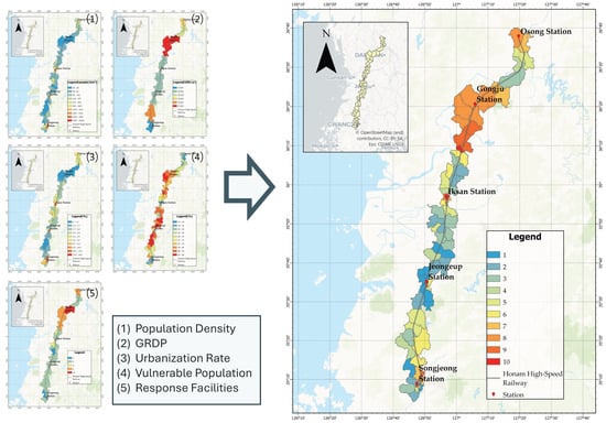
Figure 25.
Integrated spatial assessment of social vulnerability along the Honam High-Speed Railway corridor. The five submaps on the left illustrate the distribution of individual vulnerability indicators: (1) population density (persons/km2), (2) gross regional domestic product (GRDP, billion KRW), (3) urbanization rate (%), (4) the proportion of vulnerable populations (%), and (5) the availability of emergency response facilities (count). These indicators were normalized and weighted to construct a composite social vulnerability index, which is visualized in the main map on the right. Higher index values (shown in orange to red) represent areas with elevated social vulnerability. The map also marks key railway stations—Osong, Gongju, Iksan, Jeongeup, and Songjeong—to examine their proximity to highly vulnerable zones. This spatial synthesis supports risk-informed transportation planning and highlights the need for resilience measures in regions with limited adaptive capacity.
Figure 25 illustrates the spatial distribution of social vulnerability along the Honam High-Speed Railway corridor, based on five key indicators: population density, gross regional domestic product (GRDP), urbanization rate, proportion of vulnerable population, and emergency response facilities. These indicators reflect different dimensions of social vulnerability, such as demographic pressure, economic capacity, urban development, social fragility, and institutional preparedness.
The individual maps reveal regional variations in each indicator. For instance, Songjeong and Iksan show high population density and urbanization, while Osong and Gongju exhibit stronger economic productivity. Vulnerable populations are more concentrated in the southern parts of the corridor, notably around Jeongeup and Songjeong. Emergency response facilities are unevenly distributed, with some areas lacking sufficient infrastructure.
The composite vulnerability map on the right consolidates the five indicators into a single index, highlighting regions with greater overall vulnerability, such as the mid-southern corridor between Gongju and Jeongeup. These areas tend to have low economic resilience and high concentrations of vulnerable populations with limited emergency support.
The alignment of high-speed railway stations with these vulnerable areas underscores the importance of integrating vulnerability assessments into transportation planning for improved resilience and safety. This analysis highlights the need for targeted investments in infrastructure and disaster preparedness, particularly where critical transport infrastructure intersects with socially vulnerable populations.
3.3. Integrated Assessment of Hazard Exposure and Community Vulnerability
A comprehensive understanding of rail-related disaster risk requires a multidimensional analytical approach that moves beyond assessments based on a single variable. In the case of high-speed railway infrastructure, which spans large geographical areas and operates with a high degree of sensitivity to external disturbances, it is essential to evaluate both the likelihood of physical hazard occurrence and the potential severity of impacts on affected communities. This dual perspective is necessary to support the development of realistic and effective disaster response strategies.
The assessment of physical hazard focused on identifying structural vulnerabilities by analyzing spatial data related to ground subsidence, groundwater variation, railway structure classification, and train operating speeds. These indicators collectively describe the likelihood and magnitude of damage to physical infrastructure. On the other hand, the assessment of social vulnerability measured a community’s exposure and response capacity by using indicators such as population density, urban development level, regional economic output, the proportion of socially at-risk groups, including children and elderly people, and the accessibility of emergency response facilities. While each assessment highlights a distinct aspect of risk, neither is sufficient on its own to explain the full extent of potential disaster impacts, which result from the interaction between exposure to hazards and the vulnerability of the affected population.
To address this, the study conducted a Composite Community Vulnerability Assessment by spatially integrating the physical hazard index from Section 3.1 with the social vulnerability index from Section 3.2. This method allows for the identification of areas where both high hazard potential and weak social resilience overlap. The combined risk map supports disaster mitigation efforts, guides the allocation of response resources, and informs investment decisions in public infrastructure.
Both indices were standardized and mapped using the same spatial framework. This allowed the resulting map to reflect not only the possibility of hazard occurrence but also the capacity of communities to absorb and respond to those hazards. The integrated analysis provides a detailed spatial assessment that can support advanced modeling of risk in infrastructure systems that extend across long corridors. It also offers valuable insights for planning based on empirical data and for establishing long-term strategies for resilient infrastructure management. Figure 26 presents the integrated risk map derived from the overlay of the composite physical hazard and social vulnerability indices along the Honam High-Speed Railway corridor.
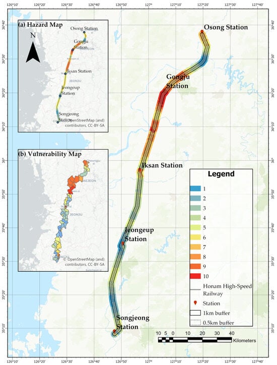
Figure 26.
Composite risk map for the Honam High-Speed Railway (HSR) corridor derived from the integration of physical hazard and social vulnerability indices. The map illustrates the spatial distribution of rail-related disaster risk based on the weighted overlay of composite hazard exposure and community vulnerability factors. Panel (a) presents the physical hazard map generated from geospatial indicators, including ground subsidence, subsidence velocity, groundwater outflow, railway structure type, and train speed. Panel (b) shows the social vulnerability map, constructed using population density, urbanization rate, GDP, proportion of vulnerable groups (children and elderly), and the accessibility of emergency facilities. The central map displays the resulting composite risk levels along the HSR line, classified into ten ordinal categories using the natural breaks method. Risk intensities are visualized along a 1 km and 0.5 km buffer zone from the railway centerline (solid and dotted lines, respectively), indicating potential impact areas in case of disaster. High-risk zones demonstrate the spatial convergence of physical hazard potential and weak social resilience. This integrated map offers a strategic basis for prioritizing mitigation efforts and informing community-level emergency planning.
Figure 26 presents the spatial synthesis of disaster risk for the Honam High-Speed Railway (HSR) corridor, integrating both physical hazard and social vulnerability dimensions. This composite risk assessment facilitates the identification of critical areas where the probability of hazardous events aligns with heightened community susceptibility.
Figure 26a illustrates the composite hazard map, developed from five key geotechnical and operational indicators: ground subsidence, subsidence velocity, groundwater outflow volume, railway structure type, and train speed. These indicators were standardized and combined using a weighted overlay based on the analytic hierarchy process (AHP) and Euclidean-based dependency adjustment. High hazard intensity is concentrated in segments near Gongju Station, reflecting a confluence of active subsidence, high-speed operation, and structurally vulnerable infrastructure.
Figure 26b displays the composite social vulnerability map, which incorporates demographic and socioeconomic variables, including population density, urbanization rate, gross regional domestic product (GRDP), proportion of vulnerable populations (under 9 and over 65), and the accessibility of emergency facilities. Higher vulnerability is observed in regions with dense populations and insufficient emergency infrastructure, particularly near Jeongeup and Gongju, where aging demographics and limited response capacity prevail.
The main map visualizes the resulting composite risk levels along the railway alignment, classified into ten ordinal categories using the natural breaks method. Risk intensities are depicted within 0.5 km (dotted line) and 1 km (solid line) buffer zones from the rail centerline, representing the potential impact areas in the event of a disaster. Notably, areas surrounding Gongju and Iksan Stations demonstrate a spatial convergence of elevated geotechnical hazards and heightened social vulnerability, designating them as priority zones for targeted risk mitigation and resilience planning. To reconcile the disparity in spatial resolution between high-resolution hazard layers and administrative-level vulnerability indicators, a buffer-based interpolation method combined with administrative overlays was applied to ensure consistent and spatially coherent risk integration along the corridor.
This integrated risk mapping framework demonstrates the value of combining technical and social assessments to inform spatially explicit, data-driven planning and investment in disaster resilience for high-speed rail infrastructure.
Figure 27 Integrated visualization of hazard and vulnerability assessment along the Honam High-Speed Railway line. Figure 27a presents the spatial distribution of hazard levels, highlighting a concentration of elevated hazard near Gongju Station. Figure 27b shows the corresponding vulnerability assessment, which similarly indicates a high-risk zone in the vicinity of Gongju Station. A representative segment with overlapping high hazard and vulnerability levels is magnified for detailed analysis. The lower portion of the figure illustrates the corresponding geotechnical and structural cross-section applied to this segment, including the upper and lower roadbeds, P.H.C. piles (500 × 80 t), soft soil treatment, sedimentary layer, and disposal area. This case exemplifies an engineering response strategy for high-risk sections of railway infrastructure.
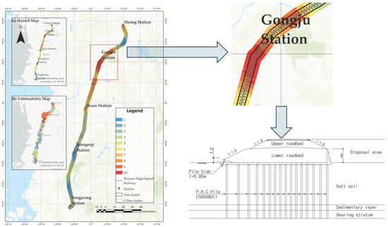
Figure 27.
Integrated visualization of hazard and vulnerability assessment along the Honam High-Speed Railway line. Panel (a) presents the spatial distribution of hazard levels, highlighting a concentration of elevated hazard near Gongju Station. Panel (b) shows the corresponding vulnerability assessment, which similarly indicates a high-risk zone in the vicinity of Gongju Station. A representative segment with overlapping high hazard and vulnerability levels is magnified for detailed analysis. The lower portion of the figure illustrates the corresponding geotechnical and structural cross-section applied to this segment, including the upper and lower roadbeds, P.H.C. piles (500 × 80 t), soft soil treatment, sedimentary layer, and disposal area. This case exemplifies an engineering response strategy for high-risk sections of railway infrastructure.
3.4. Case Analysis of High-Risk Zones Along the Honam HSR Corridor
3.4.1. Gongju Station Area
The area surrounding Gongju Station, located approximately 14 km south of the city center of Gongju in Chungcheongnam-do, is characterized by its mountainous topography, which contributes significantly to its elevated physical hazard levels. As illustrated in Figure 28, the region exhibits high scores on the hazard map, with values predominantly ranging from 8 to 10, reflecting substantial risk of ground subsidence in terms of both maximum ground deformation and deformation velocity.
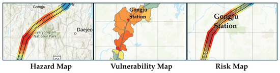
Figure 28.
Integrated hazard, vulnerability, and composite risk maps for the Gongju Station area. The hazard map (left) indicates high levels of ground deformation risk along the railway corridor near Gongju Station, particularly within mountainous terrain. The vulnerability map (center) shows relatively low to moderate social vulnerability, reflecting sparse population and minimal urban infrastructure. The composite risk map (right) reveals a localized high-risk classification (level 6), where significant physical hazard is moderated by limited social exposure.
The vulnerability map further indicates relatively high vulnerability levels, with scores between 7 and 9. Although the area’s population density and urbanization rate remain low, likely due to the mountainous landscape, other vulnerability factors—such as the limited accessibility of infrastructure, a higher proportion of elderly residents, and constrained emergency response capacity—contribute to the elevated vulnerability index.
Consequently, the composite risk map classifies the Gongju Station area as a high-risk zone, with final scores ranging from 8 to 10. This reflects the combined influence of severe physical hazards and heightened social vulnerability. From a policy perspective, this outcome underscores the need for prioritized mitigation efforts in the area. Key recommendations include the establishment of a continuous ground stability monitoring system, the implementation of protective measures for critical infrastructure, and the enhancement of response capabilities for vulnerable populations. Furthermore, the findings call for the integration of these risk assessment results into localized spatial planning and the advancement of national land safety evaluation systems to ensure proactive and context-sensitive risk management.
3.4.2. Iksan-si Area
The central area of Iksan-si in Jeollabuk-do is a highly urbanized zone characterized by dense concentrations of residential, commercial, and institutional infrastructure. As shown in Figure 29, the hazard map reveals risk levels ranging from 7 to 9 across the area, with all five hazard indicators exceeding a score of 7. This consistently elevated scoring suggests considerable geotechnical vulnerability, particularly with respect to ground instability.
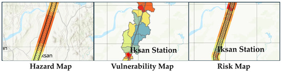
Figure 29.
Integrated hazard, vulnerability, and composite risk maps for the Iksan Station area. The hazard map (left) demonstrates moderate to high geotechnical risk (levels 7–9) associated with subsidence potential near Iksan Station. The vulnerability map (center) illustrates moderate to high levels of social vulnerability, largely driven by high population density and urbanization. The composite risk map (right) highlights several high-risk zones (levels 6–9), with localized peaks reaching level 10 due to the combination of maximum subsidence, deformation velocity, rail type, and train speed factors.
In terms of social vulnerability, the area scores high in population density and urbanization rate, while the overall vulnerability map indicates a moderate classification with values ranging from 4 to 7. These scores reflect a combination of urban intensity and variable access to emergency services and infrastructure.
The composite risk map integrates these hazard and vulnerability dimensions, indicating risk levels between 6 and 9, with certain segments marked at the maximum score of 10. These highest-risk zones are primarily associated with critical factors such as maximum ground subsidence, deformation velocity, rail type, and the maximum operational speed of trains.
From a policy and planning perspective, these findings highlight the need for comprehensive risk mitigation strategies in central Iksan. Prioritized measures should include the implementation of continuous geotechnical monitoring systems in high-risk zones, enhancement of the structural resilience of railway infrastructure, and the development of operational protocols for speed regulation in vulnerable segments. Furthermore, it is essential to integrate risk map outcomes into localized spatial planning, alongside strengthening adaptive capacity for socially vulnerable populations, to ensure effective and sustainable risk governance.
Table 10 presents the summarized assessment results for the two selected high-risk areas—Gongju Station and Iksan Station—based on hazard, vulnerability, and composite risk evaluations.
Table 10.
Summary of hazard, vulnerability, and composite risk assessment results for high-risk areas near Gongju and Iksan Stations.
4. Discussion
4.1. Methodological Contributions
This study proposes an integrated spatiotemporal risk modeling framework tailored to high-speed railway corridors by combining PS-InSAR-based ground deformation monitoring with a GIS-based multi-criteria decision-making approach. The Honam High-Speed Railway (HSR) corridor in South Korea served as a representative case study to validate the applicability of the proposed framework in identifying both geotechnical instability and spatial patterns of social vulnerability.
A core methodological innovation lies in the explicit inclusion of subsidence velocity as a dynamic hazard indicator, supplementing the conventional use of maximum vertical displacement. This dual-parameter strategy enables a more nuanced characterization of deformation risk by accounting for both the magnitude and temporal progression of ground movement—an aspect often neglected in previous assessments of linear infrastructure.
The study also introduces a correlation-adjusted analytic hierarchy process (AHP) weighting scheme that mitigates redundancy between interrelated indicators. By computing Euclidean distances between normalized indicator vectors, the influence of highly collinear inputs—such as population density and urbanization ratio—was appropriately moderated. This enhancement improves the consistency and objectivity of composite risk evaluations, especially in data-rich environments where variable interdependency is common.
Furthermore, the proposed framework adopts a segmented risk mapping approach that reflects spatial heterogeneity along the railway alignment. Unlike traditional grid-averaging techniques, this method preserves local variability in geohazard intensity and exposure, which is critical for elongated infrastructure assets where risk conditions can fluctuate substantially over short distances.
By integrating high-resolution PS-InSAR measurements with structured decision logic and adaptive segmentation, this framework offers a scalable and transferable methodology for infrastructure risk analysis. Its flexibility allows application not only to railway networks but also to other linear systems such as metro lines, highways, or utility corridors. Collectively, these methodological contributions advance the state-of-the-art in spatiotemporal risk modeling for linear infrastructure systems.
4.2. PS-InSAR Performance and Technical Limitations
However, the application of the PS InSAR technique in this study presents limitations related to the spatial distribution of corner reflectors. Although the reflectors exhibited high temporal coherence values exceeding 0.91, which ensured reliable time-series deformation measurements, the total number of installed reflectors, limited to only 17, was insufficient to accurately represent the entire 188 km extent of the Honam High-Speed Railway using inverse distance weighted interpolation. Consequently, future research should focus on establishing a more densely distributed corner reflector network in critical sections such as Gongju and Iksan, where both maximum subsidence and subsidence velocity were observed to be significant.
By implementing continuous subsidence monitoring systems in these high-risk areas, it will be possible to build a high-resolution risk analysis framework. Such an advanced monitoring infrastructure would provide objective and scientifically grounded data to support preventive measures against catastrophic accidents, such as track misalignment or train overturning caused by subsidence. Ultimately, this would play a crucial role in enhancing the safety and operational reliability of high-speed railway infrastructure.
Furthermore, the dependency-adjusted AHP weighting scheme, which accounts for indicator intercorrelation via Euclidean distance, offers a methodological advance over classical MCDM techniques. This innovation improves the reliability of risk rankings by mitigating redundancy among highly correlated inputs such as population density and urbanization ratio.
While the dependency-adjusted AHP weighting scheme improves the reliability of risk rankings by mitigating redundancy among highly correlated indicators, a fundamental methodological limitation remains: the analytic hierarchy process (AHP) inherently relies on expert judgment for pairwise comparisons. This reliance introduces an element of subjectivity, potentially affecting the consistency and reproducibility of the derived weights. In the present study, this limitation was partially addressed through a data-driven adjustment procedure that incorporated Euclidean distance-based indicator correlations. This hybrid approach aimed to balance expert knowledge with empirical interdependencies, thereby enhancing the robustness of the composite risk model. Nonetheless, future studies are encouraged to explore complementary weighting techniques—such as entropy-based methods or machine learning-driven optimization—to further minimize human-induced bias, particularly in contexts where expert consensus is limited or contested.
4.3. Hydrological Risk and Groundwater Interaction
Recent studies have increasingly highlighted the influence of long-term groundwater outflow on ground deformation in alluvial environments. For instance, ref. [105] utilized SBAS-InSAR techniques with 47 ALOS-2 (PALSAR-2) images collected between 2015 and 2021 to analyze subsidence patterns across a 21,678 km2 area in the Bohai Bay region. Their analysis identified six concentrated subsidence zones, with deformation rates reaching up to –94 mm/year. Notably, significant segments of the Beijing–Tianjin Intercity HSR (161.4 km) and the Beijing–Shanghai HSR (194.5 km) were affected, with 11–28% of the rail corridors experiencing subsidence exceeding 10 mm/year. These results underscore the spatial vulnerability of high-speed railway infrastructure in geologically sensitive alluvial plains and emphasize the importance of integrating hydrological dynamics into deformation risk assessments.
Similarly, ref. [106] utilized an SBAS-PS InSAR workflow on 292 Sentinel-1 images (2016–2022) to monitor deformation across the Choushui River alluvial plain. Their results revealed a large, centralized subsidence bowl centered on Yunlin County, with maximum deformation rates nearing 60 mm/yr. By integrating InSAR data with groundwater well logs and compaction measurements, they identified shallow aquifer (1st–2nd layer) compaction as the primary contributor to land subsidence along the Taiwan High-Speed Rail (THSR) corridor. Based on an allowable threshold of 40 mm/yr, the authors recommended managing seasonal groundwater fluctuations within 3–6 m in shallow and 4–6 m in deeper aquifers to limit ongoing consolidation. This integrated InSAR–hydrogeology framework highlights how excessive seasonal drawdown accelerates track settlement and provides actionable parameters for mitigation planning.
Beyond methodological concerns, data limitations also require consideration. In this study, groundwater variability was estimated using monthly well depth records from the national monitoring network. To ensure spatial consistency with the PS InSAR deformation analysis, only 17 observation wells located near corner reflectors were used. While this spatial alignment improved data coherence, the limited number and uneven distribution of monitoring sites may have restricted the ability to detect localized hydrological anomalies along the 188 km railway corridor.
In addition, groundwater levels were represented by monthly interpolated values, rather than direct on-site measurements throughout the entire railway section. As a result, the spatial detail and temporal sensitivity of the hydrogeological risk indicators may have been reduced. This constraint limits the ability of the model to detect rapid or localized changes in groundwater conditions, particularly in areas with complex geological variability.
Furthermore, while this study incorporated hydrogeological data to characterize groundwater-driven deformation, it did not explicitly consider climatic variables such as precipitation patterns, temperature fluctuations, or seasonal recharge cycles, all of which can significantly influence subsurface hydromechanical processes. For instance, intense rainfall events may lead to increased pore pressure and consolidation, while prolonged droughts can exacerbate aquifer drawdown and surface settlement. Temperature-induced soil expansion and contraction may also contribute to deformation, particularly in fine-grained soils. Future research should integrate meteorological datasets and climate projections to more comprehensively evaluate the coupled interactions between climatic forcing and ground subsidence risk in high-speed railway corridors.
In addition to addressing climatic drivers, improving the accuracy and responsiveness of future assessments will require the establishment of a more comprehensive groundwater monitoring network with a higher density of observation points, particularly in critical areas such as Gongju and Iksan. Incorporating continuous observation systems would further enhance the precision and reliability of groundwater-related risk assessments.
4.4. Spatial Risk Patterns Along the Honam HSR Corridor
In the Gongju area, high levels of geotechnical risk were identified due to concentrated subsidence and deformation, while social vulnerability remained low, owing to sparse population and limited development. This resulted in a moderate to high composite risk level, with the severe physical hazard offset by minimal exposure. In Iksan, concentrated urban development and population density have contributed to heightened levels of social vulnerability. When combined with moderate geotechnical hazards, this has resulted in notably elevated composite risk levels across several segments of the corridor. The interplay of ground deformation dynamics, rail infrastructure characteristics, and train operational conditions further intensifies the risk in certain areas. These findings highlight the importance of implementing targeted risk mitigation measures, such as the continuous monitoring of ground stability, the strengthening of structural components, and the application of operational controls in vulnerable sections to ensure safe and resilient railway operations.
Beyond general mitigation principles, specific engineering measures may include the reinforcement of subgrade using geosynthetic materials, the installation of settlement-monitoring sensors (e.g., inclinometers and extensometers), and the implementation of water table management systems to mitigate deformation in affected zones. In high-risk areas such as near Gongju Station, periodic track releveling and speed reduction protocols could be applied to maintain operational safety. While a formal cost–benefit analysis was not within the scope of this study, future work should evaluate the economic viability and prioritization of these interventions, particularly for long-term resilience planning under budget constraints.
4.5. Data, Modeling, and Analytical Limitations
While the proposed framework demonstrates strong potential for geospatial risk assessment of linear infrastructure, several limitations associated with data availability, modeling assumptions, and analytical precision warrant critical discussion.
First, the PS-InSAR dataset employed in this study is derived from 29 X-band SAR scenes (24 TerraSAR-X and 5 TanDEM-X acquisitions) obtained in ascending orbit mode from 2016 to 2018. While the use of high-resolution commercial satellites ensures precise displacement measurements, the relatively high cost and limited temporal availability of such data constrain long-term monitoring. Consequently, the two-year observation window used in this study allows for detecting short- to medium-term deformation signals but remains insufficient to capture long-term subsidence trends or delayed geotechnical responses to cumulative natural and anthropogenic drivers. To address this limitation, future research should consider incorporating extended temporal baselines using open-access SAR missions such as Sentinel-1 or ALOS-2, which offer continuous data streams. However, due to their coarser spatial resolution compared to TerraSAR-X, further methodological studies are required to enhance the spatial fidelity of deformation detection using medium-resolution sensors, potentially through advanced filtering techniques, resolution fusion strategies, or hybrid PS-SBAS integration frameworks.
Second, the estimation of segment-level train velocities was derived indirectly from public railway timetables and route lengths. While this approximation provided a practical basis for integrating operational dynamics into the risk model, it may introduce uncertainty due to potential discrepancies between scheduled and actual travel speeds. The integration of onboard GNSS datasets or real-time train telemetry would provide more accurate assessments of operational exposure.
Third, socioeconomic and infrastructure-related vulnerability indicators, including gross domestic product, emergency facility access, and medical infrastructure density, were aggregated at the administrative (city or county) level. This spatial generalization may have obscured localized variations in exposure and adaptive capacity, particularly in densely developed urban sub-districts or sparsely populated rural fringes. Employing finer-grained data such as census blocks or land-parcel-level statistics would improve spatial resolution and analytical precision.
The validation of PS-InSAR-derived deformation was constrained due to the limited number of available ground control points, including 17 corner reflectors and several known groundwater drawdown zones. Although these reference points provided essential ground truth for calibration, their sparse and uneven distribution limited the ability to verify deformation signals across the full 188 km extent of the corridor. This spatial limitation may reduce the robustness of the model in capturing localized subsidence features, particularly in areas without direct observational data. To enhance validation accuracy and spatial representativeness, future studies should incorporate additional geodetic control sources, such as GNSS stations or benchmark-leveling networks. Furthermore, establishing a denser groundwater observation array aligned with the rail corridor would improve the integration of hydrogeological processes into deformation risk modeling and support more reliable hazard characterization.
Moreover, the social vulnerability indicators used in this study—such as the gross domestic product, access to emergency facilities, and medical infrastructure density—were derived from 2019 statistics and do not capture temporal variations in socioeconomic conditions. This static representation may overlook evolving patterns of vulnerability driven by demographic shifts, policy changes, or infrastructure development. Incorporating multi-year datasets or time-series statistics would allow future studies to assess the dynamics of vulnerability and improve the temporal robustness of the risk model.
Finally, the use of the analytic hierarchy process (AHP) for indicator weighting, while offering a structured and transparent framework, remains sensitive to subjectivity in expert judgment. Although this limitation was partially mitigated through a data-driven adjustment procedure incorporating Euclidean distance-based dependency analysis, the influence of initial pairwise assumptions persists. Future studies should consider hybrid weighting approaches, such as fuzzy AHP, entropy weighting, or principal component analysis (PCA), to enhance objectivity and reproducibility, particularly in contexts where expert consensus is fragmented or difficult to obtain.
Collectively, addressing these limitations will be essential to refining the scalability, transferability, and empirical rigor of the proposed risk assessment framework across diverse infrastructural and geographical contexts.
4.6. Practical Applicability and Roadmap for Adaptation
Nevertheless, this study offers a scalable, extensible, and transferable framework for infrastructure risk assessment. Its reliance on open-access satellite data (e.g., SBAS, GNSS, and Lidar), modular integration of AHP-based decision logic, and compatibility with widely available GIS platforms (e.g., QGIS 3.44) ensure adaptability to a variety of geographical contexts, including rural railways, coastal corridors, or urban transit systems. To operationalize such flexibility, a six-phase conceptual roadmap was developed, encompassing (1) data acquisition and preprocessing, (2) hazard and vulnerability modeling, (3) weighting and aggregation, (4) spatial structuring, (5) risk visualization, and (6) policy-oriented application (see Figure 30). This phased structure enables users to substitute or augment modules based on local data availability and risk priorities—for instance, replacing PS-InSAR with GNSS data, or adjusting vulnerability indicators based on region-specific socioeconomic conditions.
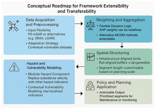
Figure 30.
Conceptual roadmap showing the modular workflow and adaptation paths for different geospatial contexts.
Furthermore, the rail-aligned segmentation strategy allows for consistent application across linear infrastructure types—including metro lines, pipelines, or highways—facilitating cross-domain risk comparisons. The framework’s modular design supports context-specific adaptation while preserving methodological consistency. As smart mobility systems and digital twins increasingly underpin transportation planning, this integrative approach enables data-driven resilience management and sustainable infrastructure governance across diverse spatial, institutional, and technical landscapes. Similar methodologies have been applied in various geospatial studies, such as flash flood vulnerability assessments in Bangladesh [107], multi-hazard risk assessments of rail infrastructure in India [108], and machine learning-based risk modeling in the Indian state of Uttarakhand [109].
Although this study primarily applies PS-InSAR due to its high precision in point-based monitoring using clearly defined scatterers such as corner reflectors, the platform is also designed to support SBAS-InSAR processing. SBAS is advantageous for spatially continuous deformation analysis and can complement PS-based assessments, especially in areas without dense artificial targets. As shown in Figure 29, the framework accommodates both approaches, allowing users to flexibly apply either or both depending on regional data availability and monitoring objectives. This dual compatibility ensures the robust long-term monitoring of rail corridors, supporting proactive risk mitigation and infrastructure sustainability.
5. Conclusions
This study presented a geospatial risk assessment framework integrating high-resolution PS-InSAR analysis with AHP-based multi-criteria modeling to identify hazard-prone segments along the Honam High-Speed Railway. The approach successfully captured ground subsidence patterns and linked them with infrastructure types and social vulnerability indicators to produce segment-level risk maps.
By incorporating TerraSAR-X and TanDEM-X imagery, the method provided spatially continuous deformation monitoring, overcoming the limitations of point-based ground methods. The dependency-adjusted AHP weighting improved the robustness of risk modeling by minimizing bias due to multicollinearity.
Key findings reveal that subsidence-prone areas like Gongju and Iksan exhibit varying risk levels, depending on both geotechnical and socioeconomic conditions. The model’s ability to account for these localized differences enables more targeted mitigation strategies.
This framework offers practical utility for adaptive infrastructure management by supporting risk-informed maintenance planning, speed regulation, and sensor deployment. Its compatibility with open-source tools also ensures scalability and transferability to other regions.
Future work should explore the integration of additional hazard types, real-time operational data, and long-term climate variability to extend the model toward a comprehensive, multi-hazard infrastructure risk platform.
Author Contributions
Conceptualization, S.-J.L., H.-S.Y. and S.-W.K.; methodology, S.-J.L. and S.-W.K.; software, S.-J.L. and S.-W.K.; validation, S.-J.L. and H.-S.Y.; formal analysis, S.-J.L. and S.-W.K.; investigation, S.-J.L. and S.-W.K.; resources, S.-J.L.; data curation, S.-J.L.; writing—original draft preparation, S.-J.L. and S.-W.K.; writing—review and editing, H.-S.Y. and S.-W.K.; visualization, S.-J.L. and S.-W.K.; supervision, H.-S.Y.; project administration, H.-S.Y.; funding acquisition, H.-S.Y. All authors have read and agreed to the published version of the manuscript.
Funding
This work was supported by a National Research Foundation of Korea (NRF) grant funded by the Korea government (MSIT) (RS-2021-NR059478).
Institutional Review Board Statement
Not applicable.
Informed Consent Statement
Not applicable.
Data Availability Statement
The SAR images used in this study were commercially purchased from Airbus Defence and Space and are not publicly available due to licensing restrictions. However, they may be shared by the corresponding author upon reasonable request for academic or research purposes.
Conflicts of Interest
The authors declare no conflicts of interest.
Appendix A
Appendix A presents supplementary outputs derived from the overall PS-InSAR processing workflow. This section includes intermediate and supporting results that, while not central to the main text, are essential for understanding the processing steps, evaluating data quality, and ensuring the reproducibility of the analysis. Figures and tables in this appendix illustrate key components such as coherence maps, reflectivity layers, interferometric connections, and time-series deformation results associated with each scene. These materials provide a comprehensive overview of the PS-InSAR implementation applied in this study.
Table A1.
Types of X-band SAR images used in this study (Scene 2).
Table A1.
Types of X-band SAR images used in this study (Scene 2).
| Scene 2: 29 Images (TerraSAR-X: 24, TanDEM-X: 5); Right-Looking (X-Band), Ascending Orbit | ||||||
|---|---|---|---|---|---|---|
| Image | Satellite | Date | Polarization | Baseline | Interval | Doppler |
| Slave | TerraSAR-X | 9 August 2016 | HH | −91.4334 | −319 | −0.03895 |
| Slave | TerraSAR-X | 20 August 2016 | HH | −210.844 | −308 | −0.01011 |
| Slave | TerraSAR-X | 11 September 2016 | HH | −94.8596 | −286 | −0.01479 |
| Slave | TerraSAR-X | 25 October 2016 | HH | −45.771 | −242 | −0.01932 |
| Slave | TerraSAR-X | 16 November 2016 | HH | −35.6862 | −220 | −0.00188 |
| Slave | TerraSAR-X | 30 December 2016 | HH | −90.1487 | −176 | −0.00235 |
| Slave | TerraSAR-X | 21 January 2017 | HH | 80.70174 | −154 | 0.007928 |
| Slave | TerraSAR-X | 12 February 2017 | HH | −40.5533 | −132 | 0.01236 |
| Slave | TerraSAR-X | 6 March 2017 | HH | 42.83211 | −110 | −0.00118 |
| Slave | TerraSAR-X | 17 March 2017 | HH | 105.1081 | −99 | −0.00223 |
| Slave | TerraSAR-X | 28 March 2017 | HH | 28.31367 | −88 | −0.00973 |
| Slave | TerraSAR-X | 19 April 2017 | HH | 125.2578 | −66 | −0.00322 |
| Slave | TerraSAR-X | 11 May 2017 | HH | −134.051 | −44 | −0.01308 |
| Slave | TerraSAR-X | 2 June 2017 | HH | −7.39436 | −22 | −0.00789 |
| Master | TerraSAR-X | 24 June 2017 | HH | 0 | 0 | −0.01849 |
| Slave | TanDEM-X | 1 October 2017 | HH | 355.9156 | 99 | −0.01324 |
| Slave | TerraSAR-X | 23 October 2017 | HH | −24.9506 | 121 | −0.01263 |
| Slave | TerraSAR-X | 14 November 2017 | HH | −211.436 | 143 | −0.00716 |
| Slave | TerraSAR-X | 6 December 2017 | HH | 56.67686 | 165 | −0.00214 |
| Slave | TanDEM-X | 28 December 2017 | HH | 284.7677 | 187 | −0.01603 |
| Slave | TanDEM-X | 30 January 2018 | HH | 22.77071 | 220 | −0.01462 |
| Slave | TanDEM-X | 4 March 2018 | HH | 154.5185 | 253 | −0.01146 |
| Slave | TerraSAR-X | 6 April 2018 | HH | 135.3632 | 286 | −0.00857 |
| Slave | TerraSAR-X | 28 April 2018 | HH | −263.041 | 308 | −0.0307 |
| Slave | TanDEM-X | 20 May 2018 | HH | 204.1424 | 330 | −0.02224 |
| Slave | TerraSAR-X | 22 June 2018 | HH | −35.0611 | 363 | −0.01708 |
| Slave | TerraSAR-X | 25 July 2018 | HH | −15.1098 | 396 | −0.02195 |
| Slave | TerraSAR-X | 27 August 2018 | HH | −52.7121 | 429 | −0.00247 |
| Slave | TerraSAR-X | 29 September 2018 | HH | 31.05214 | 462 | 0.001123 |
Table A2.
Types of X-band SAR images used in this study (Scene 3).
Table A2.
Types of X-band SAR images used in this study (Scene 3).
| Scene 3: 29 Images (TerraSAR-X: 24, TanDEM-X: 5); Right-Looking (X-Band), Ascending Orbit | ||||||
|---|---|---|---|---|---|---|
| Image | Satellite | Date | Polarization | Baseline | Interval | Doppler |
| Slave | TerraSAR-X | 3 August 2016 | HH | −168.097 | −451 | −0.02134 |
| Slave | TerraSAR-X | 25 August 2016 | HH | −102.245 | −429 | −0.01147 |
| Slave | TerraSAR-X | 16 September 2016 | HH | −85.422 | −407 | −0.01441 |
| Slave | TerraSAR-X | 8 October 2016 | HH | −81.6386 | −385 | −0.02015 |
| Slave | TerraSAR-X | 30 October 2016 | HH | −275.201 | −363 | −0.01138 |
| Slave | TerraSAR-X | 21 November 2016 | HH | −88.9957 | −341 | −0.0067 |
| Slave | TerraSAR-X | 13 December 2016 | HH | −34.3649 | −319 | −0.00669 |
| Slave | TerraSAR-X | 4 January 2017 | HH | −189.509 | −297 | 0.004638 |
| Slave | TerraSAR-X | 26 January 2017 | HH | −223.287 | −275 | 0.008062 |
| Slave | TerraSAR-X | 17 February 2017 | HH | 137.1766 | −253 | −0.01038 |
| Slave | TerraSAR-X | 11 March 2017 | HH | −52.2451 | −231 | −0.04463 |
| Slave | TerraSAR-X | 2 April 2017 | HH | 132.1616 | −209 | −0.0249 |
| Slave | TerraSAR-X | 24 April 2017 | HH | −55.8083 | −187 | −0.0081 |
| Slave | TerraSAR-X | 16 May 2017 | HH | −63.8358 | −165 | −0.01862 |
| Slave | TerraSAR-X | 7 June 2017 | HH | 32.58929 | −143 | −0.01333 |
| Slave | TerraSAR-X | 29 June 2017 | HH | −159.037 | −121 | −0.01161 |
| Slave | TerraSAR-X | 14 September 2017 | HH | −1.91879 | −44 | −0.01136 |
| Slave | TanDEM-X | 6 October 2017 | HH | 174.375 | −22 | −0.00828 |
| Master | TerraSAR-X | 28 October 2017 | HH | 0 | 0 | 0.000715 |
| Slave | TerraSAR-X | 19 November 2017 | HH | −341.748 | 22 | 0.000198 |
| Slave | TerraSAR-X | 11 December 2017 | HH | −189.382 | 44 | −0.02149 |
| Slave | TerraSAR-X | 13 January 2018 | HH | −176.582 | 76 | −0.02701 |
| Slave | TerraSAR-X | 15 February 2018 | HH | −72.0711 | 110 | −0.0138 |
| Slave | TerraSAR-X | 20 March 2018 | HH | −69.0874 | 143 | −0.00992 |
| Slave | TanDEM-X | 22 April 2018 | HH | 297.2611 | 176 | −0.00192 |
| Slave | TanDEM-X | 25 May 2018 | HH | 226.9615 | 209 | −0.0038 |
| Slave | TerraSAR-X | 27 June 2018 | HH | −222.357 | 242 | −0.02135 |
| Slave | TerraSAR-X | 30 July 2018 | HH | −37.3414 | 275 | −0.02406 |
| Slave | TanDEM-X | 1 September 2018 | HH | 118.3237 | 308 | −0.00499 |
Table A3.
Types of X-band SAR images used in this study (Scene 4).
Table A3.
Types of X-band SAR images used in this study (Scene 4).
| Scene 4: 29 Images (TerraSAR-X: 24, TanDEM-X: 5); Right-Looking (X-Band), Ascending Orbit | ||||||
|---|---|---|---|---|---|---|
| Image | Satellite | Date | Polarization | Baseline | Interval | Doppler |
| Slave | TerraSAR-X | 3 August 2016 | HH | −104.485 | −286 | −0.02134 |
| Slave | TerraSAR-X | 25 August 2016 | HH | −39.3234 | −264 | −0.01147 |
| Slave | TerraSAR-X | 16 September 2016 | HH | −21.8271 | −242 | −0.01441 |
| Slave | TerraSAR-X | 8 October 2016 | HH | −19.1595 | −220 | −0.02015 |
| Slave | TerraSAR-X | 30 October 2016 | HH | −211.989 | −198 | −0.01138 |
| Slave | TerraSAR-X | 21 November 2016 | HH | −26.0299 | −176 | −0.0067 |
| Slave | TerraSAR-X | 13 December 2016 | HH | 30.03268 | −154 | −0.00669 |
| Slave | TerraSAR-X | 4 January 2017 | HH | −126.541 | −132 | 0.004638 |
| Slave | TerraSAR-X | 26 January 2017 | HH | −159.611 | −110 | 0.008062 |
| Slave | TerraSAR-X | 17 February 2017 | HH | 200.3253 | −88 | −0.01038 |
| Slave | TerraSAR-X | 11 March 2017 | HH | 11.37803 | −66 | −0.04463 |
| Slave | TerraSAR-X | 2 April 2017 | HH | 195.2449 | −44 | −0.0249 |
| Slave | TerraSAR-X | 24 April 2017 | HH | 8.21256 | −22 | −0.0081 |
| Master | TerraSAR-X | 16 May 2017 | HH | 0 | 0 | −0.01862 |
| Slave | TerraSAR-X | 7 June 2017 | HH | 96.97956 | 22 | −0.01333 |
| Slave | TerraSAR-X | 29 June 2017 | HH | −95.744 | 44 | −0.01161 |
| Slave | TerraSAR-X | 14 September 2017 | HH | 61.11293 | 121 | −0.01136 |
| Slave | TanDEM-X | 6 October 2017 | HH | 237.993 | 143 | −0.00828 |
| Slave | TerraSAR-X | 28 October 2017 | HH | 62.80535 | 165 | 0.000715 |
| Slave | TerraSAR-X | 19 November 2017 | HH | −278.284 | 187 | 0.000198 |
| Slave | TerraSAR-X | 11 December 2017 | HH | −126.26 | 209 | −0.02149 |
| Slave | TerraSAR-X | 13 January 2018 | HH | −112.882 | 242 | −0.02701 |
| Slave | TerraSAR-X | 15 February 2018 | HH | −8.27112 | 275 | −0.0138 |
| Slave | TerraSAR-X | 20 March 2018 | HH | −6.02228 | 308 | −0.00992 |
| Slave | TanDEM-X | 22 April 2018 | HH | 360.8435 | 341 | −0.00192 |
| Slave | TanDEM-X | 25 May 2018 | HH | 291.7482 | 374 | −0.0038 |
| Slave | TerraSAR-X | 27 June 2018 | HH | −158.312 | 407 | −0.02135 |
| Slave | TerraSAR-X | 30 July 2018 | HH | 26.54346 | 440 | −0.02406 |
| Slave | TanDEM-X | 1 September 2018 | HH | 181.7141 | 473 | −0.00499 |

Figure A1.
Backscatter maps of the four TerraSAR-X/TanDEM-X scenes covering the Honam High-Speed Railway corridor. Each grayscale image represents radar intensity after the coregistration of 28 slave images to a master scene. Bright areas indicate strong radar reflectivity (e.g., urban infrastructure), while darker areas correspond to low-reflectivity surfaces such as vegetation, water bodies, or rugged terrain.


Figure A2.
Scatter plot of cumulative ground displacement derived from PS-InSAR time-series analysis over Scene 1-1 along the Honam High-Speed Railway corridor. The x-axis and y-axis represent pixel coordinates in range (Lines [pix]) and azimuth (Samples [pix]) directions, respectively. Each dot corresponds to a persistent scatterer (PS) point, colored by cumulative vertical displacement (in mm) during the observation period (August 2016 to September 2018). Negative values (in red tones) indicate ground subsidence, while positive values (in blue tones) represent uplift. The displacement range spans from approximately −45 mm to +45 mm. This figure offers a detailed view of localized deformation behavior within the most displacement-prone segment (Scene 1-1) discussed in Section 3.1.1, and it complements the broader subsidence patterns presented in the main text.


Figure A3.
Scatter plot of cumulative ground displacement derived from PS-InSAR time-series analysis over Scene 1-2 along the Honam High-Speed Railway corridor. The x-axis and y-axis represent pixel coordinates in range (Lines [pix]) and azimuth (Samples [pix]) directions, respectively. Each dot corresponds to a persistent scatterer (PS) point, colored by cumulative vertical displacement (in mm) during the observation period (August 2016 to September 2018). Negative values (in red tones) indicate ground subsidence, while positive values (in blue tones) represent uplift. The displacement range spans from approximately −45 mm to +45 mm. This figure offers a detailed view of localized deformation behavior within the most displacement-prone segment (Scene 1-2) discussed in Section 3.1.1, and it complements the broader subsidence patterns presented in the main text.


Figure A4.
Scatter plot of cumulative ground displacement derived from PS-InSAR time-series analysis over Scene 2 along the Honam High-Speed Railway corridor. The x-axis and y-axis represent pixel coordinates in range (Lines [pix]) and azimuth (Samples [pix]) directions, respectively. Each dot corresponds to a persistent scatterer (PS) point, colored by cumulative vertical displacement (in mm) during the observation period (August 2016 to September 2018). Negative values (in red tones) indicate ground subsidence, while positive values (in blue tones) represent uplift. The displacement range spans from approximately −45 mm to +45 mm. This figure offers a detailed view of localized deformation behavior within the most displacement-prone segment (Scene 3-1) discussed in Section 3.1.1, and it complements the broader subsidence patterns presented in the main text.


Figure A5.
Scatter plot of cumulative ground displacement derived from PS-InSAR time-series analysis over Scene 3-1 along the Honam High-Speed Railway corridor. The x-axis and y-axis represent pixel coordinates in range (Lines [pix]) and azimuth (Samples [pix]) directions, respectively. Each dot corresponds to a persistent scatterer (PS) point, colored by cumulative vertical displacement (in mm) during the observation period (August 2016 to September 2018). Negative values (in red tones) indicate ground subsidence, while positive values (in blue tones) represent uplift. The displacement range spans from approximately −45 mm to +45 mm. This figure offers a detailed view of localized deformation behavior within the most displacement-prone segment (Scene 3-2) discussed in Section 3.1.1, and it complements the broader subsidence patterns presented in the main text.


Figure A6.
Scatter plot of cumulative ground displacement derived from PS-InSAR time-series analysis over Scene 3-2 along the Honam High-Speed Railway corridor. The x-axis and y-axis represent pixel coordinates in range (Lines [pix]) and azimuth (Samples [pix]) directions, respectively. Each dot corresponds to a persistent scatterer (PS) point, colored by cumulative vertical displacement (in mm) during the observation period (August 2016 to September 2018). Negative values (in red tones) indicate ground subsidence, while positive values (in blue tones) represent uplift. The displacement range spans from approximately −45 mm to +45 mm. This figure offers a detailed view of localized deformation behavior within the most displacement-prone segment (Scene 4-1) discussed in Section 3.1.1, and it complements the broader subsidence patterns presented in the main text.


Figure A7.
Scatter plot of cumulative ground displacement derived from PS-InSAR time-series analysis over Scene 4–1 along the Honam High-Speed Railway corridor. The x-axis and y-axis represent pixel coordinates in range (Lines [pix]) and azimuth (Samples [pix]) directions, respectively. Each dot corresponds to a persistent scatterer (PS) point, colored by cumulative vertical displacement (in mm) during the observation period (August 2016 to September 2018). Negative values (in red tones) indicate ground subsidence, while positive values (in blue tones) represent uplift. The displacement range spans from approximately −45 mm to +45 mm. This figure offers a detailed view of localized deformation behavior within the most displacement-prone segment (Scene 4-2) discussed in Section 3.1.1, and it complements the broader subsidence patterns presented in the main text.


Figure A8.
Scatter plot of cumulative ground displacement derived from PS-InSAR time-series analysis over Scene 4–2 along the Honam High-Speed Railway corridor. The x-axis and y-axis represent pixel coordinates in range (Lines [pix]) and azimuth (Samples [pix]) directions, respectively. Each dot corresponds to a persistent scatterer (PS) point, colored by cumulative vertical displacement (in mm) during the observation period (August 2016 to September 2018). Negative values (in red tones) indicate ground subsidence, while positive values (in blue tones) represent uplift. The displacement range spans from approximately −45 mm to +45 mm. This figure offers a detailed view of localized deformation behavior within the most displacement-prone segment (Scene 4-2) discussed in Section 3.1.1, and it complements the broader subsidence patterns presented in the main text.

Appendix B
This appendix provides detailed descriptions and classification criteria for the nine non-InSAR indicators used in the composite risk assessment model. Each indicator was normalized and categorized into ten ordinal levels using Jenks’s natural breaks optimization. The table below summarizes the definition, data source, measurement unit, and classification thresholds for each indicator, including population density, GDP per capita, urbanization ratio, vulnerable population ratio, the accessibility of emergency facilities, groundwater variability, the railway track type, the operational speed, and the design train speed. These parameters formed the vulnerability and hazard input layers used in the AHP-based spatial risk evaluation.

Figure A9.
Comparison of PS-InSAR-derived subsidence (blue line) with precise leveling data (red points with error bars) for sites 2 through 9. The horizontal axis represents the profile distance (m), and the vertical axis indicates displacement (mm). Overall, the PS-InSAR measurements show good agreement with the ground-truth leveling results, with site-specific deviations depending on local conditions.


Figure A10.
Comparison of PS-InSAR-derived subsidence (blue line) with precise leveling data (red points with error bars) for sites 10 through 17. The horizontal axis represents the profile distance (m), and the vertical axis indicates displacement (mm). Overall, the PS-InSAR measurements show good agreement with the ground-truth leveling results, with site-specific deviations depending on local conditions.


Figure A11.
Corner reflector (CR) installation and geometric configuration for PS-InSAR monitoring along the Honam High-Speed Railway. (a) Location of the CR site near the Honam HSR line (36.1665° N, 127.0503° E), with a zoomed-in satellite image highlighting the precise reflector placement north of Gwangju–Songjeong Station. (b) Ground-level photographs of the CR installed on a concrete platform in an open field with minimal vegetation to ensure reliable backscatter. The compactness of the CR is 0.91, indicating high geometric precision. (c) Geometric alignment between the CR and satellite imaging parameters, including satellite orbit heading angle (190.37°), CR opening direction (100.37°), flight direction, and look direction. The TanDEM-X satellite operates at an altitude of approximately 514 km with an orbital inclination of 97.44° and a revisit cycle of 11 days. It transmits and receives X-band microwave signals toward the lower right of its orbital path.

Table A4.
Geographic coordinates of 63 bridges included in the Honam High-Speed Railway corridor analysis. Structure-specific weights were assigned based on the extended AHP methodology outlined in Section 2.3 and subsequently interpolated using the IDW method, as visualized in Figure 6. Bridge structures represent one of three classified railway structure types—alongside tunnels and embankments—and were assigned an AHP-derived weight of 3.23, reflecting their relative vulnerability to ground deformation.
| Bridge Name | Lon (°E) | Lat (°N) | Bridge Name | Lon (°E) | Lat (°N) | Bridge Name | Lon (°E) | Lat (°N) |
|---|---|---|---|---|---|---|---|---|
| Osong Overpass | 127.3206 | 36.61778 | Taeseong Overpass | 127.3064 | 36.60059 | Sansu Bridge | 127.2656 | 36.55384 |
| Geumgang Bridge | 127.2338 | 36.51007 | Buyong Bridge | 127.2168 | 36.48518 | Hwangryong Overpass | 127.2036 | 36.46707 |
| Balsan Overpass | 127.1746 | 36.42738 | Maam Bridge | 127.275 | 36.55803 | Bongmyeong Overpass | 127.2717 | 36.55438 |
| Bongmyeong Bridge | 127.269 | 36.55113 | Hyangji Ramyeon Bridge | 127.2682 | 36.5503 | Hyangji Bridge | 127.2674 | 36.54939 |
| Sinyeong No. 1 Bridge | 127.1044 | 36.34302 | Sinyeong No. 2 Bridge | 127.103 | 36.34092 | Sinyeong No. 3 Bridge | 127.1016 | 36.33883 |
| Sinyeong No. 4 Bridge | 127.1001 | 36.33673 | Gongju Overpass | 127.0968 | 36.33245 | Sinyeongcheon Bridge | 127.0943 | 36.32878 |
| Hoam Bridge | 127.0788 | 36.28572 | Seopyeon Bridge | 127.0692 | 36.27005 | Janggu Bridge | 127.0533 | 36.24424 |
| Ogang Bridge | 127.0459 | 36.20076 | Sindang Bridge | 127.0402 | 36.18662 | Galsan Bridge | 127.0258 | 36.16373 |
| Jeongji Overpass | 127.0131 | 36.1158 | Jeongji Bridge | 127.0066 | 36.09582 | Sinjak Bridge | 126.9803 | 36.03084 |
| Eoryang Bridge (1) | 126.9573 | 35.98692 | Eoryang Bridge (2) | 126.9543 | 35.98144 | Hwabae Bridge | 126.9403 | 35.95302 |
| Hwasil Bridge | 126.9474 | 35.94588 | Juksan Bridge | 126.9225 | 35.85903 | Jungni Bridge | 126.9096 | 35.81996 |
| Wonhyeong No. 1 Bridge | 126.8984 | 35.77739 | Wonhyeong No. 2 Bridge | 126.8962 | 35.76899 | Wonhyeong No. 3 Bridge | 126.892 | 35.7552 |
| Hwangdeung No. 1 Bridge | 126.8885 | 35.7425 | Hwangdeung No. 2 Bridge | 126.8853 | 35.73251 | Hwangdeung No. 3 Bridge | 126.8787 | 35.71353 |
| Mokcheon Bridge | 126.876 | 35.70462 | Mangyeonggang Bridge | 126.8694 | 35.68649 | Yongam Overpass | 126.8593 | 35.65842 |
| Buyong No. 1 Overpass | 126.8524 | 35.63975 | Buyong No. 2 Overpass | 126.85 | 35.63328 | Duwol Overpass | 126.8431 | 35.61466 |
| Gangjeong Overpass | 126.8382 | 35.59989 | Wonpyeongcheon Bridge | 126.8344 | 35.58854 | Yujeong Bridge | 126.8204 | 35.52989 |
| Yeonjeong Bridge | 126.8107 | 35.49394 | Gyuchon Bridge | 126.8038 | 35.46264 | Wolsong Bridge | 126.8004 | 35.44456 |
| Hankyocheon Bridge | 126.8247 | 35.42469 | Namsan Bridge | 126.8177 | 35.41092 | Jeongeup Overpass | 126.8079 | 35.38148 |
| Eupjicheon Bridge | 126.8057 | 35.37276 | Daeheung Overpass | 126.8145 | 35.33798 | Yongheung Overpass | 126.8033 | 35.28991 |
| Hwangryong No. 1 Bridge | 126.805 | 35.23144 | Hwangryong No. 2 Bridge | 126.8061 | 35.22283 | Waryongcheon Bridge | 126.809 | 35.20161 |
| Maryeong No. 1 Overpass | 126.8118 | 35.18298 | Maryeong No. 2 Overpass | 126.813 | 35.17213 | Hwangryonggang Bridge | 126.7938 | 35.12482 |
| Osong Overpass | 127.3206 | 36.61778 | Taeseong Overpass | 127.3064 | 36.60059 | Sansu Bridge | 127.2656 | 36.55384 |
| Geumgang Bridge | 127.2338 | 36.51007 | Buyong Bridge | 127.2168 | 36.48518 | Hwangryong Overpass | 127.2036 | 36.46707 |
| Balsan Overpass | 127.1746 | 36.42738 | Maam Bridge | 127.275 | 36.55803 | Bongmyeong Overpass | 127.2717 | 36.55438 |
| Bongmyeong Bridge | 127.269 | 36.55113 | Hyangji Ramyeon Bridge | 127.2682 | 36.5503 | Hyangji Bridge | 127.2674 | 36.54939 |
| Sinyeong No. 1 Bridge | 127.1044 | 36.34302 | Sinyeong No. 2 Bridge | 127.103 | 36.34092 | Sinyeong No. 3 Bridge | 127.1016 | 36.33883 |
| Sinyeong No. 4 Bridge | 127.1001 | 36.33673 | Gongju Overpass | 127.0968 | 36.33245 | Sinyeongcheon Bridge | 127.0943 | 36.32878 |
Table A5.
Geographic coordinates of 34 tunnels along the Honam High-Speed Railway corridor. Structure-specific weights were assigned to each tunnel section using the extended analytic hierarchy process (AHP) methodology described in Section 2.3. These weights reflect the relative susceptibility of tunnel segments to ground deformation and were integrated into the spatial vulnerability assessment presented in Figure 6.
| Tunnel Name | Lon (°E) | Lat (°N) | Tunnel Name | Lon (°E) | Lat (°N) | Tunnel Name | Lon (°E) | Lat (°N) |
|---|---|---|---|---|---|---|---|---|
| Hakcheon Tunnel | 127.2827 | 36.57495 | Galsan Tunnel | 127.2366 | 36.51075 | Buyong Tunnel 1 | 127.2144 | 36.47918 |
| Buyong Tunnel 2 | 127.2046 | 36.46501 | Jangjae Tunnel | 127.1872 | 36.43815 | Yeonggok Tunnel | 127.1558 | 36.39389 |
| Gyeryong Tunnel | 127.124 | 36.3484 | Wondong Tunnel | 127.0788 | 36.28572 | Bongmyeong Tunnel | 127.055 | 36.24519 |
| Hyangji Tunnel | 127.0459 | 36.20076 | Yeomcheon Tunnel | 127.032 | 36.17281 | Sinyeong Tunnel | 127.0131 | 36.1158 |
| Noti Tunnel | 126.9803 | 36.03084 | Mogaul Tunnel | 126.9522 | 35.97672 | Jungni Tunnel | 126.9474 | 35.94588 |
| Gimje Cut-and-Cover | 126.9225 | 35.85903 | Hoeryong Tunnel | 126.8998 | 35.77368 | Usan Tunnel | 126.8886 | 35.74394 |
| Noryeong Tunnel | 126.8349 | 35.5114 | Dalseong Tunnel | 126.8292 | 35.4821 | Jukcheong Tunnel | 126.8249 | 35.45538 |
| Seongdeok Tunnel 1 | 126.8163 | 35.39834 | Seongdeok Tunnel 2 | 126.8157 | 35.39389 | Moam Tunnel | 126.8145 | 35.33798 |
| Songhyeon Tunnel 1 | 126.8058 | 35.27694 | Songhyeon Tunnel 2 | 126.8049 | 35.26827 | Songhyeon Tunnel 3 | 126.8039 | 35.2596 |
| Jangsan Tunnel | 126.803 | 35.25094 | Yongheung Tunnel | 126.802 | 35.24227 | Waryong Tunnel 1 | 126.805 | 35.23144 |
| Waryong Tunnel 2 | 126.8077 | 35.20907 | Maryeong Tunnel | 126.8124 | 35.16632 | Sinryong Tunnel | 126.7994 | 35.14771 |
| Goryong Tunnel | 126.7975 | 35.13903 |

Figure A12.
Spatial distribution of administrative regions corresponding to place names listed in Table A6. The map displays the location and extent of each administrative unit used in the PS-InSAR analysis across the study area, subdivided into three panels. Each yellow polygon is labeled with a unique identifier matching the numeric codes in Table A6. These codes represent local administrative divisions (eup, myeon, and dong) within the Honam High-Speed Railway corridor and surrounding regions.

Table A6.
Regional demographic and economic indicators used as input factors for the community vulnerability mapping. The variables include total population, area, gross regional domestic product (GRDP), age-based vulnerable groups (under 9 and over 65 years old), and urbanization rate. These indicators were integrated into the vulnerability index to assess spatial disparities along the Honam High-Speed Railway corridor.
| Region No. | Region | Population | Area (km2) | GRDP ($) | Under 9 Age (Population) | Over 65 Age (Population) | Urbanization Rate (%) |
|---|---|---|---|---|---|---|---|
| 1 | O-song-eup | 20,823 | 63,050,646 | 30,503 | 2696 | 2354 | 4 |
| 2 | Gangnae-myeon | 13,594 | 46,805,483 | 30,503 | 1723 | 765 | 3 |
| 3 | Iin-myeon | 3183 | 97,400,173 | 37,053 | 1223 | 113 | 1 |
| 4 | Gyeryong-myeon | 5360 | 129,672,457 | 37,053 | 1976 | 181 | 1 |
| 5 | Banpo-myeon | 4223 | 92,717,968 | 37,053 | 1081 | 161 | 1 |
| 6 | Ganggyeong-eup | 8804 | 10,810,760 | 37,053 | 2551 | 395 | 6 |
| 7 | Seongdong-myeon | 4472 | 54,502,954 | 37,053 | 1594 | 104 | 2 |
| 8 | Gwangseok-myeon | 4267 | 52,604,574 | 37,053 | 1543 | 134 | 2 |
| 9 | Noseong-myeon | 3182 | 55,258,836 | 37,053 | 1111 | 141 | 2 |
| 10 | Chaeun-myeon | 2203 | 30,307,889 | 37,053 | 835 | 76 | 2 |
| 11 | Hamyeol-eup | 7147 | 29,098,804 | 20,596 | 2120 | 375 | 4 |
| 12 | Hwangdeung-myeon | 6984 | 42,400,332 | 20,596 | 2142 | 294 | 3 |
| 13 | Nangsan-myeon | 3031 | 53,502,144 | 20,596 | 1067 | 119 | 2 |
| 14 | Mangseong-myeon | 3074 | 49,218,113 | 20,596 | 1215 | 84 | 2 |
| 15 | Samgi-myeon | 2612 | 35,736,342 | 20,596 | 892 | 72 | 3 |
| 16 | Yongdong-myeon | 1548 | 25,585,725 | 20,596 | 689 | 22 | 2 |
| 17 | Pyeonghwa-dong | 5096 | 9,886,521 | 20,596 | 986 | 339 | 5 |
| 18 | Inhwa-dong | 7150 | 3,702,896 | 20,596 | 1894 | 367 | 11 |
| 19 | Ma-dong | 9676 | 2,297,636 | 20,596 | 1157 | 105 | 13 |
| 20 | Namjung-dong | 12,482 | 2,701,479 | 20,596 | 3372 | 502 | 17 |
| 21 | Mohyeon-dong | 38,098 | 5,267,182 | 20,596 | 5181 | 3973 | 12 |
| 22 | Songhak-dong | 8512 | 2,204,911 | 20,596 | 1231 | 980 | 10 |
| 23 | Sin-dong | 23,936 | 19,008,948 | 20,596 | 3342 | 716 | 5 |
| 24 | Samseong-dong | 31,789 | 19,571,625 | 20,596 | 3208 | 2823 | 4 |
| 25 | Sintaein-eup | 5444 | 45,591,363 | 20,596 | 1906 | 279 | 2 |
| 26 | Ibam-myeon | 2658 | 54,423,634 | 20,596 | 1125 | 62 | 2 |
| 27 | Jeongu-myeon | 2430 | 46,099,490 | 20,596 | 1039 | 85 | 2 |
| 28 | Taein-myeon | 3421 | 51,994,311 | 20,596 | 1378 | 107 | 2 |
| 29 | Gamgok-myeon | 2658 | 63,489,582 | 20,596 | 1193 | 53 | 2 |
| 30 | Suseong-dong | 17,985 | 8,942,096 | 20,596 | 2298 | 1709 | 9 |
| 31 | Chosan-dong | 10,965 | 4,265,108 | 20,596 | 1530 | 951 | 6 |
| 32 | Yeonji-dong | 5375 | 2,590,866 | 20,596 | 1282 | 421 | 12 |
| 33 | Nongso-dong | 4155 | 28,574,526 | 20,596 | 1077 | 186 | 3 |
| 34 | Sanggyo-dong | 3767 | 70,188,931 | 20,596 | 1441 | 146 | 1 |
| 35 | Baeksan-myeon | 2321 | 44,876,964 | 20,596 | 911 | 63 | 3 |
| 36 | Yongji-myeon | 3588 | 53,201,765 | 20,596 | 1388 | 113 | 2 |
| 37 | Baekgu-myeon | 3843 | 33,740,600 | 20,596 | 1373 | 126 | 3 |
| 38 | Gongdeok-myeon | 2392 | 44,064,184 | 20,596 | 943 | 75 | 2 |
| 39 | Bongnam-myeon | 2086 | 36,110,308 | 20,596 | 951 | 53 | 2 |
| 40 | Hwangsan-myeon | 1887 | 27,735,488 | 20,596 | 755 | 41 | 3 |
| 41 | Yochon-dong | 10,984 | 16,881,724 | 20,596 | 2665 | 809 | 6 |
| 42 | Sinpung-dong | 13,198 | 35,037,663 | 20,596 | 2771 | 988 | 3 |
| 43 | Geomsan-dong | 11,690 | 21,760,627 | 20,596 | 1781 | 1108 | 4 |
| 44 | Jangseong-eup | 13,181 | 104,324,886 | 31,001 | 3284 | 1029 | 2 |
| 45 | Nam-myeon | 3222 | 42,354,097 | 31,001 | 1020 | 172 | 2 |
| 46 | Hwangnyong-myeon | 3840 | 67,387,074 | 31,001 | 1081 | 171 | 2 |
| 47 | Seosam-myeon | 1388 | 51,320,708 | 31,001 | 495 | 58 | 1 |
| 48 | Bugil-myeon | 1210 | 46,058,461 | 31,001 | 518 | 34 | 1 |
| 49 | Bugi-myeon | 2675 | 84,932,347 | 31,001 | 1131 | 82 | 1 |
| 50 | Yeondong-myeon | 3573 | 33,483,820 | 25,573 | 1014 | 119 | 3 |
| 51 | Bugang-myeon | 6553 | 43,661,950 | 25,573 | 1354 | 386 | 3 |
| 52 | Geumnam-myeon | 8812 | 112,030,802 | 25,573 | 2389 | 320 | 1 |
| 53 | Bangok-dong | 8676 | 29,892,367 | 25,573 | 286 | 1531 | 3 |
| 54 | Songjeong dong (1) | 11,407 | 2213,484 | 19,856 | 1669 | 822 | 7 |
| 55 | Songjeong dong (2) | 6537 | 2,033,599 | 19,856 | 1367 | 350 | 17 |
| 56 | Dosan-dong | 15,897 | 6,159,194 | 19,856 | 1898 | 1607 | 4 |
| 57 | Sinheul-dong | 4791 | 8,165,533 | 19,856 | 827 | 383 | 2 |
| 58 | Eoryong-dong | 35,933 | 26,534,338 | 19,856 | 2696 | 2354 | 4 |
| 59 | Usan-dong | 24,656 | 6,906,728 | 19,856 | 1723 | 765 | 9 |
| 60 | Wolgok dong (1) | 13,523 | 962,596 | 19,856 | 1223 | 113 | 17 |
| 61 | Wolgok dong (2) | 23,454 | 1,503,231 | 19,856 | 1976 | 181 | 15 |
| 62 | Hanam-dong | 26,325 | 23,591,385 | 19,856 | 1081 | 161 | 13 |
| 63 | Imgok-dong | 2055 | 44,497,510 | 19,856 | 2551 | 395 | 1 |
| 64 | Donggok-dong | 1888 | 24,083,367 | 19,856 | 1594 | 104 | 2 |
| 65 | Pyeong-dong | 6440 | 43,246,774 | 19,856 | 1543 | 134 | 6 |
| 66 | Pyeong-dong | 6440 | 17,061,780 | 25,760 | 1111 | 141 | 6 |
| 67 | Tancheon-myeon | 3204 | 99,132,588 | 37,053 | 835 | 76 | 1 |
| 68 | Chochon-myeon | 2217 | 42,790,682 | 37,053 | 2120 | 375 | 2 |
| 69 | Jungang-dong | 3229 | 1,351,615 | 20,596 | 2142 | 294 | 18 |
| 70 | Deokcheon-myeon | 1764 | 31,331,044 | 20,596 | 1067 | 119 | 2 |
| 71 | Unnam-dong | 31,772 | 4,150,754 | 19,856 | 1215 | 84 | 9 |
| 72 | Suwan-dong | 77,979 | 6,910,368 | 19,856 | 892 | 72 | 14 |
Appendix C
The following images illustrate the high-resolution PS-InSAR data obtained through TerraSAR-X imagery, which was commercially procured for the study. The figures below represent the areas covered by the acquired satellite data.
Figure A13: Overview of the study area, with the highlighted region indicating the focus of the analysis.
Figure A14: Detailed imagery of the study area, showcasing the high-resolution data collected by TerraSAR-X and TanDEM.
These datasets are available for further research purposes. If required, interested researchers may contact the corresponding author to request access to the raw data for academic and non-commercial purposes.

Figure A13.
Overview of the study area along the Honam High-Speed Railway corridor, showing the geographical region covered by the TerraSAR-X image. The red box indicates the area of interest for the PS-InSAR analysis, while the inset map provides the location of the study area within South Korea. The acquisition date and other relevant metadata are also provided, including the product type and orbital parameters.


Figure A14.
High-resolution TerraSAR-X image of the study area along the Honam High-Speed Railway corridor, showcasing the detailed spatial distribution of surface features. This satellite imagery was utilized in the PS-InSAR analysis to assess ground displacement and monitor subsidence along the railway infrastructure. The image provides critical insights into both urban and natural terrain, which were analyzed for potential geotechnical risks related to ground deformation.

Appendix D
To structure a comprehensive and scalable framework for railway infrastructure risk analysis, this study employs the analytic hierarchy process (AHP), which enables systematic decomposition of complex decision problems into a hierarchical structure consisting of the goal, criteria, sub-criteria, and alternatives. The approach is particularly well suited to evaluating composite risks that emerge from interactions between geotechnical hazards and urban vulnerability conditions, especially in transport networks and smart city corridors.
Originally developed by Thomas Saaty in the 1980s, AHP is a multi-criteria decision-making (MCDM) method designed to handle both quantitative and qualitative factors through pairwise comparisons and eigenvalue-based weighting [9]. The methodology has been widely applied in urban planning, infrastructure management, and disaster risk assessment contexts [110,111]. While AHP assumes factor independence within each hierarchy level, this study addresses the known limitation of horizontal interdependencies by introducing a dependency adjustment mechanism in Section 2.3.2.
To estimate the relative importance of decision-making elements and assess the consistency of pairwise comparisons, AHP derives a matrix of comparisons between all criteria. This process yields a consistent weighting scheme through eigenvalue calculations. For a set of n evaluation factors (A1, A2, …, Aₙ) with corresponding weights (W1, W2, …, Wₙ), the pairwise comparison matrix A is structured as follows:
While the eigenvalue method enables the calculation of the relative importance of decision-making elements based on pairwise comparisons, the AHP framework inherently evaluates alternatives two at a time. Consequently, the resulting priority ranking is not always guaranteed to be consistent when interpreted through transitive relationships among three or more elements. To address this limitation, the present study employs the consistency ratio (CR) to validate the reliability of expert judgments in the pairwise comparison matrix. According to Saaty, a CR value below 0.1 is considered acceptably consistent, while values between 0.1 and 0.2 are marginally acceptable depending on context. Values exceeding 0.2 are deemed unacceptably inconsistent and require judgment revision.
To ensure the validity of the analytic hierarchy process (AHP) application, this study grounded its methodological framework on four essential theoretical assumptions, as summarized in Table A7. These assumptions serve as the foundational criteria for structuring pairwise comparisons and constructing a consistent hierarchical model.
Table A7.
Theoretical Assumptions of AHP.
Table A7.
Theoretical Assumptions of AHP.
| Addressed Assumption | Description |
|---|---|
| Reciprocity | All decision elements must be mutually comparable, and the degree of importance should be measurable in a reciprocal manner. |
| Homogeneity | The compared elements should fall within a limited range, with a common scale to allow meaningful evaluation. |
| Independence | While elements in a lower layer depend on their immediate upper-level criteria, horizontal independence among peer elements must be maintained. |
| Expectation | The hierarchy must fully represent the scope of decision-makers’ rational expectations, covering all relevant aspects of the problem. |
However, in practical applications, these assumptions may be challenged by inconsistencies in questionnaire design or respondent interpretation. To address potential violations, this study incorporated specific mitigation strategies, as shown in Table A8.
Table A8.
Mitigation Measures to Satisfy AHP Assumptions.
Table A8.
Mitigation Measures to Satisfy AHP Assumptions.
| Addressed Assumption | Mitigation Strategy |
|---|---|
| Reciprocity | All pairwise questions were standardized using the following format to ensure consistency: “How much more important is subsidence factor A compared to B?” |
| Homogeneity | A dimensionless 10-point scale was adopted to unify judgment standards and eliminate scale disparity. |
| Independence | Criteria and sub-criteria were selected to be mutually exclusive and logically distinct, minimizing redundancy. |
| Expectation | The hierarchical model was limited to two levels to reduce complexity and facilitate accurate expert judgments. |
To construct a pairwise comparison matrix suitable for the analytic hierarchy process (AHP), expert respondents were asked to compare the relative importance of each factor with respect to others in a structured questionnaire format. Table A9 illustrates a portion of the survey used in this study. Each question follows a standardized phrasing—“How important do you think Factor X is compared to Factor Y?”—and utilizes Saaty’s fundamental scale ranging from 1/9 to 9 to quantify preference strength.
Table A9.
Example structure of the AHP-based pairwise comparison questionnaire used for multi-criteria decision analysis. Each question prompts respondents to evaluate the relative importance of one factor over another using a standardized scale.
Table A9.
Example structure of the AHP-based pairwise comparison questionnaire used for multi-criteria decision analysis. Each question prompts respondents to evaluate the relative importance of one factor over another using a standardized scale.
| Question No. | Pairwise Comparison | Scale Selection Example |
|---|---|---|
| 1 | How important do you think Factor 1 is compared to Factor 2? | 1/3 |
| 2 | How important do you think Factor 1 is compared to Factor 3? | 1/2 |
| ⋮ | ⋮ | ⋮ |
| 10 | How important do you think Factor 4 is compared to Factor 5? | 1 |
The responses collected from the survey are then aggregated and used to generate the pairwise comparison matrix A, where each element aij represents the relative importance of Factor i over Factor j. An example matrix based on five evaluation criteria is shown in Table A10.
Table A10.
Example of a pairwise comparison matrix constructed for risk assessment using the analytic hierarchy process (AHP). The matrix reflects the relative importance of the five factors based on expert judgment, forming the basis for deriving priority weights.
Table A10.
Example of a pairwise comparison matrix constructed for risk assessment using the analytic hierarchy process (AHP). The matrix reflects the relative importance of the five factors based on expert judgment, forming the basis for deriving priority weights.
| Factor 1 | Factor 2 | Factor 3 | Factor 4 | Factor 5 | |
|---|---|---|---|---|---|
| Factor 1 | 1 | 0.333 | 0.5 | 1 | 0.5 |
| Factor 2 | 3 | 1 | 2 | 2 | 1 |
| Factor 3 | 2 | 0.5 | 1 | 1 | 1 |
| Factor 4 | 1 | 0.5 | 1 | 1 | 0.5 |
| Factor 5 | 2 | 1 | 1 | 2 | 1 |
This matrix became the basis for deriving the normalized weight vector and calculating consistency metrics, including the consistency index (CI) and the consistency ratio (CR), as part of the AHP process.
To evaluate the relative importance of risk factors associated with railway infrastructure and surrounding socioeconomic vulnerability, this study adopted the analytic hierarchy process (AHP). The methodology was applied to a set of ten key indicators: five related to geotechnical and operational risk, namely ground subsidence magnitude, subsidence rate, groundwater outflow volume, track type, and section speed, and five related to community vulnerability, comprising population density, regional GDP, urbanization rate, the proportion of vulnerable groups, and the presence of relief facilities.
In the initial AHP hierarchy, all ten indicators were assessed using expert-driven pairwise comparisons on a unified 10-point Saaty scale. However, certain qualitative or categorical indicators, specifically track type, urbanization rate, and the availability of relief facilities, could not be directly stratified within the main hierarchy due to their inherent limitations in continuous scaling. As a result, a second-stage AHP analysis was performed for these three indicators. This subhierarchical evaluation enabled a refined and context-sensitive weighting process, ensuring the analytical consistency and comparability of all final indicator weights within the overall decision framework.
References
- Ferretti, A.; Prati, C.; Rocca, F. Permanent Scatterers in SAR Interferometry. IEEE Trans. Geosci. Remote Sens. 2001, 39, 8–20. [Google Scholar] [CrossRef]
- Akcin, H.A.K.A.N.; Kutoglu, H.S.; Kemaldere, H.; Deguchi, T.; Koksal, E. Monitoring subsidence effects in the urban area of Zonguldak Hardcoal Basin of Turkey by InSAR-GIS integration. Nat. Hazards Earth Syst. Sci. 2010, 10, 1807–1814. [Google Scholar] [CrossRef]
- Shahzad, F.; Zhu, Z.; Gloaguen, R. Monitoring Land Subsidence in the Peshawar District, Pakistan, with a Multi-Track PS-InSAR Technique. Nat. Hazards Earth Syst. Sci. 2010, 10, 1807–1815. [Google Scholar] [CrossRef]
- Khan, J.; Ren, X.; Hussain, M.A.; Jan, M.Q. Monitoring Land Subsidence Using PS-InSAR Technique in Rawalpindi and Islamabad, Pakistan. Remote Sens. 2022, 14, 3722. [Google Scholar] [CrossRef]
- Mohamadi, B.; Abu Ghazala, M.O.; Li, H.; Al-Sabbagh, T.A.; Younes, A. Integrating InSAR Coherence and Air Pollution Detection Satellites to Study the Impact of War on Air Quality. Int. J. Appl. Earth Obs. Geoinf. 2025, 142, 104687. [Google Scholar] [CrossRef]
- Mohamadi, B.; Balz, T.; Younes, A. A Model for Complex Subsidence Causality Interpretation Based on PS-InSAR Cross-Heading Orbits Analysis. Remote Sens. 2019, 11, 2014. [Google Scholar] [CrossRef]
- Chai, L.; Xie, X.; Wang, C.; Tang, G.; Song, Z. Ground subsidence risk assessment method using PS-InSAR and LightGBM: A case study of Shanghai metro network. Int. J. Digit. Earth 2024, 17, 2297842. [Google Scholar] [CrossRef]
- Kyriou, A.; Mpelogianni, V.; Nikolakopoulos, K.; Groumpos, P.P. Review of Remote Sensing Approaches and Soft Computing for Infrastructure Monitoring. Geomatics 2023, 3, 367–392. [Google Scholar] [CrossRef]
- Saaty, T.L. The Analytic Hierarchy Process; McGraw-Hill: New York, NY, USA, 1980. [Google Scholar]
- Malczewski, J. GIS and Multicriteria Decision Analysis; John Wiley & Sons: New York, NY, USA, 2006. [Google Scholar]
- Lyu, H.; Yin, Z. An improved MCDM combined with GIS for risk assessment of multi-hazards in Hong Kong. Sustain. Cities Soc. 2023, 96, 104427. [Google Scholar] [CrossRef]
- Devara, M.; Tiwari, A.; Dwivedi, R. Landslide susceptibility mapping using MT-InSAR and AHP enabled GIS-based multi-criteria decision analysis. Geomat. Nat. Hazards Risk 2021, 12, 675–693. [Google Scholar] [CrossRef]
- Sar, N.; Chatterjee, S.; Das Adhikari, M. Integrated remote sensing and GIS based spatial modelling through analytical hierarchy process (AHP) for water logging hazard, vulnerability and risk assessment in Keleghai river basin, India. Model. Earth Syst. Environ. 2015, 1, 31. [Google Scholar] [CrossRef]
- Lyu, H.-M.; Shen, S.-L.; Zhou, A.; Yang, J. Risk assessment of mega-city infrastructures related to land subsidence using improved trapezoidal FAHP. Sci. Total Environ. 2020, 717, 135310. [Google Scholar] [CrossRef] [PubMed]
- Biscaya, S.; Elkadi, H. A smart ecological urban corridor for the Manchester Ship Canal. Cities 2021, 110, 103042. [Google Scholar] [CrossRef]
- Elkadi, H.; Biscaya, S. Towards a smart ecological urban corridor for Manchester Ship Canal. In Proceedings of the ICSC 2018: 20th International Conference on Smart Cities, Bangkok, Thailand, 13–14 December 2018. [Google Scholar]
- Martin, C.; Evans, J.; Karvonen, A.; Paskaleva, K.; Yang, D.; Linjordet, T. Smart-sustainability: A new urban fix? Sustain. Cities Soc. 2019, 45, 87–97. [Google Scholar] [CrossRef]
- Gracias, J.; Parnell, G.; Specking, E.; Pohl, E.; Buchanan, R. Smart Cities—A Structured Literature Review. Smart Cities 2023, 6, 1719–1743. [Google Scholar] [CrossRef]
- Lim, Y.; Edelenbos, J.; Gianoli, A. Identifying the results of smart city development: Findings from systematic literature review. Cities 2019, 95, 102397. [Google Scholar] [CrossRef]
- Santosa, H.; Fauziah, N. Establishing public consensus through developing spatial multimedia system towards smart governance in managing cityscape planning. PEOPLE Int. J. Soc. Sci. 2019, 4, 1083–1100. [Google Scholar] [CrossRef]
- Jiang, H. Smart urban governance in the ‘smart’ era: Why is it urgently needed? Cities 2020, 97, 103004. [Google Scholar] [CrossRef]
- De Falco, S.; Angelidou, M.; Addie, J.P.D. From the “smart city” to the “smart metropolis”? Building resilience in the urban periphery. Eur. Urban Reg. Stud. 2018, 26, 205–223. [Google Scholar] [CrossRef]
- Luque-Ayala, A.; Marvin, S. Developing a critical understanding of smart urbanism? Urban Stud. 2015, 52, 2105–2116. [Google Scholar] [CrossRef]
- Lee, S.-J.; Yun, H.-S.; Kim, T.-Y. Monitoring of High-Speed Railway Ground Deformation Using Interferometric Synthetic Aperture Radar Image Analysis. Appl. Sci. 2025, 15, 4318. [Google Scholar] [CrossRef]
- Chosun Ilbo. Subsidence Found in 217 Spots over 29 km of Honam High-Speed Rail. Chosun Ilbo, 13 February 2015. Available online: https://www.chosun.com/site/data/html_dir/2015/02/13/2015021300328.html (accessed on 20 March 2025).
- Korea National Railway. Ground Subsidence in Honam High-Speed Rail; Korea National Railway: Seoul, Republic of Korea, 2015; Available online: https://www.kr.or.kr/boardCnts/view.do?boardID=52&boardSeq=1101458&page=207 (accessed on 20 March 2025).
- Crosetto, M.; Monserrat, O.; Cuevas-González, M.; Crippa, B.; Devanthéry, N. Persistent Scatterer Interferometry: A Review. ISPRS J. Photogramm. Remote Sens. 2016, 115, 78–89. [Google Scholar] [CrossRef]
- Hooper, A.; Zebker, H.; Segall, P.; Kampes, B. A New Method for Measuring Deformation on Volcanoes and Other Natural Terrains Using InSAR Persistent Scatterers. Geophys. Res. Lett. 2012, 39, L09303. [Google Scholar] [CrossRef]
- Nashashibi, A.Y.; Ibrahim, A.A.; Cook, S.; Sarabandi, K. Experimental Characterization of Polarimetric Radar Backscatter Response of Distributed Targets at High Millimeter-Wave Frequencies. IEEE Trans. Geosci. Remote Sens. 2016, 54, 1013–1024. [Google Scholar] [CrossRef]
- Alaqeel, A.A.; Douglas, T.J.; Nashashibi, A.Y.; Sarabandi, K. J-Band Polarimetric Radar Measurements of Surfaces at High Angles of Incidence. IEEE Trans. Geosci. Remote Sens. 2024, 62, 5106612. [Google Scholar] [CrossRef]
- Baghdadi, N.; Choker, M.; Zribi, M.; El Hajj, M.; Paloscia, S.; Verhoest, N.E.C.; Lievens, H.; Baup, F.; Mattia, F. A New Empirical Model for Radar Scattering from Bare Soil Surfaces. Remote Sens. 2016, 8, 920. [Google Scholar] [CrossRef]
- Xu, Q.; Zhao, C.; Chen, Z.; Wu, S.; Wang, X.; Fan, L. Characterization of 77 GHz Radar Backscattering from Sea Surfaces at Low Incidence Angles: Preliminary Results. Remote Sens. 2025, 17, 116. [Google Scholar] [CrossRef]
- Meng, T.; Yang, X.; Chen, K.-S.; Nunziata, F.; Xie, D.; Buono, A. Radar Backscattering Over Sea Surface Oil Emulsions: Simulation and Observation. IEEE Trans. Geosci. Remote Sens. 2021, 60, 2000714. [Google Scholar] [CrossRef]
- Touzi, R.; Lopes, A.; Bruniquel, J.; Vachon, P.W. Coherence estimation for SAR imagery. IEEE Trans. Geosci. Remote Sens. 1999, 37, 135–149. [Google Scholar] [CrossRef]
- Aiazzi, B.; Alparone, L.; Baronti, S.; Garzelli, A. Coherence estimation from multilook incoherent SAR imagery. IEEE Trans. Geosci. Remote Sens. 2003, 41, 2531–2539. [Google Scholar] [CrossRef]
- Liang, R.; Liu, Y.; Xu, H.; Li, Z. A Novel Coherence Estimation Method for InSAR. In Proceedings of the 8th Asia-Pacific Conference on Synthetic Aperture Radar (APSAR), Bali, Indonesia, 23–27 October 2023. [Google Scholar] [CrossRef]
- Wang, M.; Huang, G.; Zhang, J.; Hua, F. A Weighted Coherence Estimator for SAR Coherent Change Detection. IEEE Trans. Geosci. Remote. Sens. 2022, 60, 5228912. [Google Scholar] [CrossRef]
- Adam, N. SAR Coherence Estimation by Composition of Subsample Estimates and Machine Learning. IEEE J. Sel. Top. Appl. Earth Obs. Remote Sens. 2024, 17, 15957–15970. [Google Scholar] [CrossRef]
- ESA. Part A: Guidelines for SAR Interferometry Processing and Interpretation. In InSAR Principles: Guidelines for SAR Interferometry Processing and Interpretation; ESA TM-19A; European Space Agency: Noordwijk, The Netherlands, 2007; Available online: https://www.esa.int/esapub/tm/tm19/TM-19_ptA.pdf (accessed on 26 July 2025).
- ESA. Part B: InSAR Processing—A Practical Approach. In InSAR Principles: Guidelines for SAR Interferometry Processing and Interpretation; ESA TM-19B; European Space Agency: Noordwijk, The Netherlands, 2007; Available online: https://www.esa.int/esapub/tm/tm19/TM-19_ptB.pdf (accessed on 26 July 2025).
- Fernández-Torres, E.A.; Cabral-Cano, E.; Novelo-Casanova, D.A.; Solano-Rojas, D.; Havazli, E.; Salazar-Tlaczani, L. Risk assessment of land subsidence and associated faulting in Mexico City using InSAR. Nat. Hazards 2022, 112, 37–55. [Google Scholar] [CrossRef]
- Zhang, Z.; Zhang, S.; Hu, C.; Zhang, X.; Yang, S.; Yan, H.; Zhang, Z. Hazard assessment model of ground subsidence coupling AHP, RS and GIS—A case study of Shanghai. Gondwana Res. 2023, 117, 344–362. [Google Scholar] [CrossRef]
- Lenardón Sánchez, M.; Farías, C.A.; Cigna, F. Multi-Decadal Land Subsidence Risk Assessment at Major Italian Cities by Integrating PSInSAR with Urban Vulnerability. Land 2024, 13, 2103. [Google Scholar] [CrossRef]
- Yu, B.; Yan, J.; Li, Y.; Xing, H. Risk Assessment of Multi-Hazards in Hangzhou: A Socioeconomic and Risk Mapping Approach Using the CatBoost-SHAP Model. Int. J. Disaster Risk Sci. 2024, 15, 640–656. [Google Scholar] [CrossRef]
- Aerts, J.P.M.; Uhlemann-Elmer, S.; Eilander, D.; Ward, P.J. Global Flood Hazard Map and Exposed GDP Comparison: A China Case Study. Nat. Hazards Earth Syst. Sci. 2020, 20, 3245–3260. [Google Scholar] [CrossRef]
- Xin, D.; Daniell, J.E.; Zhang, Z.; Wenzel, F.; Wang, S.; Chen, X. A grid-level fixed-asset model developed for China from 1951 to 2020. Nat. Hazards Earth Syst. Sci. 2025, 25, 1597–1613. [Google Scholar] [CrossRef]
- Kummu, M.; Kosonen, M.; Masoumzadeh, S. Downscaled gridded global dataset for GDP per capita (PPP) over 1990–2022. Sci. Data 2025, 12, 187. [Google Scholar] [CrossRef] [PubMed]
- Eberenz, S.; Stocker, D.; Röösli, T.; Bresch, D.N. Asset exposure data for global physical risk assessment. Earth Syst. Sci. Data 2020, 12, 817–833. [Google Scholar] [CrossRef]
- Hu, H.; Zhu, J.; Fu, H.; Liu, Z.; Xie, Y.; Liu, K. Automated Estimation of Sub-Canopy Topography Combined with Single-Baseline Single-Polarization TanDEM-X InSAR and ICESat-2 Data. Remote Sens. 2024, 16, 1155. [Google Scholar] [CrossRef]
- Hassler, J.; Granberg, T.A.; Steins, K.; Ceccato, V. Towards more realistic measures of accessibility to emergency departments in Sweden. Int. J. Health Geogr. 2024, 23, 6. [Google Scholar] [CrossRef] [PubMed]
- Kiran, K.C.; Corcoran, J.; Chhetri, P. Measuring the spatial accessibility to fire stations using enhanced floating catchment method. Socio-Econ. Plan. Sci. 2018, 68, 100667. [Google Scholar] [CrossRef]
- Nainggolan, L.; Ni, C.F.; Darmawan, Y.; Lo, W.C.; Lee, I.H.; Lin, C.P.; Hiep, N.H. Cost-effective groundwater potential mapping by integrating multiple remote sensing data and the index–overlay method. Remote Sens. 2024, 16, 502. [Google Scholar] [CrossRef]
- Erdin, C.; Çağlar, M. Rural fire risk assessment in GIS environment using fuzzy logic and the AHP approaches. Pol. J. Environ. Stud. 2021, 30, 4337–4346. [Google Scholar] [CrossRef]
- Chai, L.; Wei, L.; Cai, P.; Liu, J.; Kang, J.; Zhang, Z. Risk Assessment of Land Subsidence Based on GIS in the Yongqiao Area, Suzhou City, China. Sci. Rep. 2024, 14, 11377. [Google Scholar] [CrossRef]
- Dikmen, I.; Birgonul, M.T. An Analytic Hierarchy Process Based Model for Risk and Opportunity Assessment of International Construction Projects. Can. J. Civ. Eng. 2006, 33, 58–68. [Google Scholar] [CrossRef]
- Yahaya, S.; Ahmad, N.; Abdalla, R.F. Multicriteria analysis for flood vulnerable areas in Hadejia-Jama’are River Basin, Nigeria. Eur. J. Sci. Res. 2010, 42, 71–83. [Google Scholar]
- Sum, R.M. Risk management decision-making: The analytic hierarchy process approach. J. Int. Bus. Entrep. Dev. 2015, 8, 108–127. [Google Scholar] [CrossRef]
- Ouma, Y.O.; Tateishi, R. Urban flood vulnerability and risk mapping using integrated multi-parametric AHP and GIS. Water 2014, 6, 1515–1545. [Google Scholar] [CrossRef]
- Danumah, J.H.; Nkrumah, P.N.; Odai, S.N. Flood risk assessment and mapping in Abidjan district using multi-criteria analysis (AHP) model. Geoenviron. Disasters 2016, 3, 10. [Google Scholar] [CrossRef]
- Zhang, Z.; Wang, M.; Hu, J. Earthquake risk assessment in seismically active areas of Qinghai Province based on geographic big data. Atmosphere 2024, 15, 648. [Google Scholar] [CrossRef]
- Avci, İ.; Koca, M. A novel security risk analysis using the AHP method in smart railway systems. Appl. Sci. 2024, 14, 4243. [Google Scholar] [CrossRef]
- Sharma, A.; Miyazaki, H. Multi-hazard risk assessment in urban planning and development using AHP. ISPRS Arch. 2019, XLII-3/W8, 363–370. [Google Scholar] [CrossRef]
- Abdelkarim, A.; Elkhrachy, I.; Alzahrani, M.; Hasan, M. Integration of GIS-based multicriteria decision analysis and AHP to assess flood hazard on a train pathway. Water 2020, 12, 1702. [Google Scholar] [CrossRef]
- Bouramdane, A.A. Enhancing disaster management in smart cities through MCDM-AHP analysis amid 21st century challenges. Inf. Syst. Smart City 2024, 3, 189. [Google Scholar] [CrossRef]
- Zhuang, G. Research on safety risk assessment method of highway bridge construction based on AHP-fuzzy comprehensive evaluation. E3S Web Conf. 2021, 248, 03020. [Google Scholar] [CrossRef]
- Li, Q.; Zhou, J.; Feng, J. Safety risk assessment of highway bridge construction based on cloud entropy power method. Appl. Sci. 2022, 12, 8692. [Google Scholar] [CrossRef]
- Halder, R.K.; Uddin, M.N.; Uddin, M.A.; Aryal, S.; Khraisat, A. A comprehensive review and performance analysis of k-nearest neighbor search and join methods for high-dimensional data. J. Big Data 2024, 11, 65. [Google Scholar] [CrossRef]
- Aladayleh, K.J.; Aladaileh, M.J. Applying analytical hierarchy process (AHP) to BIM-based risk management for optimal performance in construction projects. Buildings 2024, 14, 3632. [Google Scholar] [CrossRef]
- He, J.; Dong, S. Research on contract risk management of hospital construction project based on fuzzy analytic hierarchy process. Int. J. Biol. Life Sci. 2024, 7, 79–85. [Google Scholar] [CrossRef]
- Liu, H.-H.; Yeh, Y.-Y.; Huang, J.-J. Correlated Analytic Hierarchy Process. Math. Probl. Eng. 2014, 2014, 961714. [Google Scholar] [CrossRef]
- Huang, J.-J. Analytic Hierarchy Process with the Correlation Effect via WordNet. Mathematics 2021, 9, 872. [Google Scholar] [CrossRef]
- Szádoczki, Z.; Duleba, S. Distance-based aggregation in group AHP. J. Decis. Syst. 2022, 31 (Suppl. S1), 98–106. [Google Scholar] [CrossRef]
- Ray, G.; Barney, J.B.; Muhanna, W.A. Capabilities, business processes, and competitive advantage: Choosing the dependent variable in empirical tests of the resource-based view. Strateg. Manag. J. 2003, 24, 1037–1049. [Google Scholar] [CrossRef]
- Rao, R.V.; Singh, D.; Bleicher, F.; Dorn, C. Weighted Euclidean Distance-Based Approach as a Multiple Attribute Decision Making Method for Manufacturing Situations. Int. J. Multicriteria Decis. Mak. 2012, 2, 225–240. [Google Scholar] [CrossRef]
- Chen, Z.; Zhang, X.; Lee, J. Combining PCA–AHP Combination Weighting to Prioritize Design Elements of Intelligent Wearable Masks. Sustainability 2023, 15, 1888. [Google Scholar] [CrossRef]
- Ayalew, L.; Yamagishi, H.; Ugawa, N. Landslide Susceptibility Mapping Using GIS-Based Weighted Linear Combination: The Case in Tsugawa Area of Agano River, Niigata Prefecture, Japan. Landslides 2004, 1, 73–81. [Google Scholar] [CrossRef]
- Bhattacharya, G.; Ghosh, K.; Chowdhury, A.S. Granger Causality Driven AHP for Feature Weighted kNN. Pattern Recognit. 2017, 66, 425–436. [Google Scholar] [CrossRef]
- Moslem, S.; Pilla, F. Planning Location of Parcel Lockers Using Group Analytic Hierarchy Process in Spherical Fuzzy Environment. Transp. Res. Interdiscip. Perspect. 2024, 24, 101024. [Google Scholar] [CrossRef]
- Mathew, M.; Chakrabortty, R.K.; Ryan, M.J. A Novel Approach Integrating AHP and TOPSIS under Spherical Fuzzy Sets for Advanced Manufacturing System Selection. Eng. Appl. Artif. Intell. 2020, 96, 103988. [Google Scholar] [CrossRef]
- Saeidi, A.; Deck, O.; Verdel, T. Development of building vulnerability functions in subsidence regions from empirical methods. Eng. Struct. 2009, 31, 2275–2286. [Google Scholar] [CrossRef]
- Negulescu, C.; Foerster, E. Parametric studies and quantitative assessment of the vulnerability of a RC frame building exposed to differential settlements. Nat. Hazards Earth Syst. Sci. 2010, 10, 1781–1792. [Google Scholar] [CrossRef]
- Chambers, R. Editorial introduction: Vulnerability, coping and policy. IDS Bull. 1989, 20, 1–7. [Google Scholar] [CrossRef]
- Chen, Q.; Chen, L.; Gui, L.; Yin, K.; Shrestha, D.P.; Du, J.; Cao, X. Assessment of the physical vulnerability of buildings affected by slow-moving landslides. Nat. Hazards Earth Syst. Sci. 2020, 20, 2547–2565. [Google Scholar] [CrossRef]
- Jaiswal, P.; van Westen, C.J.; Jetten, V. Quantitative assessment of direct and indirect landslide risk along transportation lines in southern India. Nat. Hazards Earth Syst. Sci. 2010, 10, 1253–1267. [Google Scholar] [CrossRef]
- Wu, Y.; Liu, D.; Lu, X.; Song, Q. Vulnerability assessment model for hazard-bearing bodies and landslide risk index. Rock Soil Mech. 2011, 32, 2487–2493, (In Chinese with English Abstract). [Google Scholar]
- Totschnig, R.; Sedlacek, W.; Fuchs, S. A quantitative vulnerability function for fluvial sediment transport. Nat. Hazards 2011, 58, 681–703. [Google Scholar] [CrossRef]
- Del Soldato, M.; Bianchini, S.; Calcaterra, D.; De Vita, P.; Di Martire, D.; Tomás, R.; Casagli, N. A new approach for landslide-induced damage assessment. Geomat. Nat. Hazards Risk 2017, 8, 1524–1537. [Google Scholar] [CrossRef]
- Mavrouli, O.; Giannopoulos, P.G.; Carbonell, J.M.; Syrmakezis, C. Damage analysis of masonry structures subjected to rockfalls. Landslides 2017, 14, 891–904. [Google Scholar] [CrossRef]
- Lee, J.-S.; Song, C.-H.; Pradhan, A.M.S.; Ha, Y.-S.; Kim, Y.-T. Development of structural type-based physical vulnerability curves to debris flow using numerical analysis and regression model. Int. J. Disaster Risk Reduct. 2024, 106, 104431. [Google Scholar] [CrossRef]
- Tajima, F.; Kageyama, T.; Nakamura, T.; Ito, K.; Kawanakajima, H.; Sakata, A. Evaluating the Cumulative Settlement of Railway Embankments Constructed with Tunnel Spoil. Transp. Eng. 2025, 20, 100307. [Google Scholar] [CrossRef]
- Liu, X.; Xiao, J.; Cai, D.; Su, Q.; Yang, G.; Yuan, S.; Jiang, G. Recent Advances in Subgrade Engineering for High-Speed Railway. Intell. Transp. Infrastruct. 2023, 2, liad001. [Google Scholar] [CrossRef]
- Jin, B.; Zeng, T.; Wang, T.; Zhang, Z.; Gui, L.; Yin, K.; Zhao, B. Advanced risk assessment framework for land subsidence impacts on transmission towers in Salt Lake region. Environ. Model. Softw. 2024, 177, 106058. [Google Scholar] [CrossRef]
- Karimai, K.; Takada, S.; Sugiyama, H.; Honsho, K. Prediction and factor analysis of liquefaction ground subsidence based on machine-learning techniques. Appl. Sci. 2024, 14, 2713. [Google Scholar] [CrossRef]
- Shults, R.; Gritsuk, D.; Yavorskyi, V.; Shults, S. Analysis of overpass displacements due to subway construction land subsidence using machine learning. Urban Sci. 2023, 7, 100. [Google Scholar] [CrossRef]
- Schotten, R.; Bachmann, D. Cataloging and Testing Flood Risk Management Measures to Increase the Resilience of Critical Infrastructure Networks. Smart Cities 2024, 7, 2995–3021. [Google Scholar] [CrossRef]
- Chen, C.; Yu, Y.-H.; Lee, Y.-F. Multi-Criteria Evaluation for Flood Risk Management Using the MCE-RISK Model. Water 2016, 8, 151. [Google Scholar] [CrossRef]
- Wang, Y.; Hong, H.; Chen, W.; Li, S.; Pamučar, D.; Gigović, L.; Duan, H. A hybrid GIS multi-criteria decision-making method for flood susceptibility mapping at Shangyou, China. Remote Sens. 2018, 11, 62. [Google Scholar] [CrossRef]
- Meena, S.R.; Mishra, B.K.; Tavakkoli Piralilou, S. A Hybrid Spatial Multi-Criteria Evaluation Method for Mapping Landslide Susceptible Areas in Kullu Valley, Himalayas. Geosciences 2019, 9, 156. [Google Scholar] [CrossRef]
- Parizi, M.K.; Osanloo, M.; Khalilzadeh, M. A GIS-based multi-criteria analysis framework to evaluate urban physical resilience against earthquakes. Sustainability 2022, 14, 5034. [Google Scholar] [CrossRef]
- Oliveira de Sousa, T.; de Oliveira, G.D.; Silva, B.C.; Salles, L.M.; Andrade, A.S. Multi-criteria assessment of flood risk on railroads using a machine learning approach: A case study of railroads in Minas Gerais. Infrastructures 2025, 10, 12. [Google Scholar] [CrossRef]
- Sarkar, T.; Sarkar, D.; Mondal, P. Road Network Accessibility Analysis Using Graph Theory and GIS Technology: A Study of the Villages of English Bazar Block, India. Spat. Inf. Res. 2021, 29, 405–415. [Google Scholar] [CrossRef]
- Groundwater Information Center. Korea National Groundwater Information System. Available online: https://www.gims.go.kr/igis_jihasumap.do (accessed on 7 May 2025).
- Korean Statistical Information Service (KOSIS). Population and Housing Census Statistics. Available online: http://kosis.kr (accessed on 7 May 2025).
- Environmental Geographic Information Service (EGIS). Ministry of Environment, Korea. Available online: https://egis.me.go.kr (accessed on 7 May 2025).
- Luo, Q.; Li, M.; Yin, Z.; Ma, P.; Perissin, D.; Zhang, Y. Land Subsidence Velocity and High-Speed Railway Risks in the Coastal Cities of Beijing–Tianjin–Hebei, China, with 2015–2021 ALOS PALSAR-2 Multi-Temporal InSAR Analysis. Remote Sens. 2024, 16, 4774. [Google Scholar] [CrossRef]
- Nguyen, T.V.; Lin, S.-J.; Yu, H.-L.; Wu, J.-C. Quantitative Assessment of Land Subsidence and Its Hydrogeological Drivers in the Choushui River Alluvial Fan Using Sentinel-1 Time-Series InSAR. Remote Sens. 2024, 16, 3789. [Google Scholar] [CrossRef]
- Sarker, S.; Jahan, I.; Wang, X.; Azad, A. Geospatial approach to assess flash flood vulnerability in a coastal district of Bangladesh: Integrating the multifaceted dimension of vulnerabilities. ISPRS Int. J. Geo-Inf. 2025, 14, 194. [Google Scholar] [CrossRef]
- Joshi, D.; Takeuchi, W.; Kumar, N.; Avtar, R. Multi-hazard risk assessment of rail infrastructure in India under local vulnerabilities towards adaptive pathways for disaster-resilient infrastructure planning. Prog. Disaster Sci. 2024, 20, 100308. [Google Scholar] [CrossRef]
- Chauhan, V.; Gupta, L.; Dixit, J. Machine learning and GIS-based multi-hazard risk modeling for Uttarakhand: Integrating seismic, landslide, and flood susceptibility with socioeconomic vulnerability. Indic. J. Geoinf. 2025, 3, 100664. [Google Scholar] [CrossRef]
- Aminbakhsh, S.; Gunduz, M.; Sonmez, R. Safety Risk Assessment Using Analytic Hierarchy Process (AHP) During Planning and Budgeting of Construction Projects. J. Saf. Res. 2013, 46, 99–105. [Google Scholar] [CrossRef]
- Cagno, E.; Caron, F.; Mancini, M. An Algorithm for the Implementation of Safety Improvement Programs. Reliab. Eng. Syst. Saf. 2000, 67, 255–269. [Google Scholar] [CrossRef]


Disclaimer/Publisher’s Note: The statements, opinions and data contained in all publications are solely those of the individual author(s) and contributor(s) and not of MDPI and/or the editor(s). MDPI and/or the editor(s) disclaim responsibility for any injury to people or property resulting from any ideas, methods, instructions or products referred to in the content. |
© 2025 by the authors. Licensee MDPI, Basel, Switzerland. This article is an open access article distributed under the terms and conditions of the Creative Commons Attribution (CC BY) license (https://creativecommons.org/licenses/by/4.0/).