Article

Landscape Ecological Risk Assessment of Peri-Urban Villages in the Yangtze River Delta Based on Ecosystem Service Values

1
College of Art and Design, Nanjing Forestry University, Nanjing 210037, China
2
College of Landscape Architecture, Nanjing Forestry University, Nanjing 210037, China
*
Author to whom correspondence should be addressed.
Sustainability 2025, 17(15), 7014; https://doi.org/10.3390/su17157014
Submission received: 23 June 2025 / Revised: 25 July 2025 / Accepted: 31 July 2025 / Published: 1 August 2025

Abstract

The rapid urbanization process has accelerated the degradation of ecosystem services (ESs) in peri-urban rural areas of the Yangtze River Delta (YRD), leading to increasing landscape ecological risks (LERs). Establishing a scientifically grounded landscape ecological risk assessment (LERA) system and corresponding control strategies is therefore imperative. Using rural areas of Jiangning District, Nanjing as a case study, this research proposes an optimized dual-dimensional coupling assessment framework that integrates ecosystem service value (ESV) and ecological risk probability. The spatiotemporal evolution of LER in 2000, 2010, and 2020 and its key driving factors were further studied by using spatial autocorrelation analysis and geodetector methods. The results show the following: (1) From 2000 to 2020, cultivated land remained dominant, but its proportion decreased by 10.87%, while construction land increased by 26.52%, with minimal changes in other land use types. (2) The total ESV increased by CNY 1.67 × 10⁹, with regulating services accounting for over 82%, among which water bodies contributed the most. (3) LER showed an overall increasing trend, with medium- to highest-risk areas expanding by 55.37%, lowest-risk areas increasing by 10.10%, and lower-risk areas decreasing by 65.48%. (4) Key driving factors include landscape vulnerability, vegetation coverage, and ecological land connectivity, with the influence of distance to road becoming increasingly significant. This study reveals the spatiotemporal evolution characteristics of LER in typical peri-urban villages. Based on the LERA results, combined with terrain features and ecological pressure intensity, the study area was divided into three ecological management zones: ecological conservation, ecological restoration, and ecological enhancement. Corresponding zoning strategies were proposed to guide rural ecological governance and support regional sustainable development.

1. Introduction

With the coordinated advancement of China’s urbanization and rural revitalization strategies [1], especially in the Yangtze River Delta (YRD) region, profound changes are taking place in the rural spatial structure and ecological pattern. As vital providers of ecosystem services (ESs), rural areas play a key role in food production, soil conservation, biodiversity maintenance, and landscape regulation [2]. Among them, peri-urban villages, situated at the interface between urban expansion and natural ecosystems, have long faced challenges such as intensive resource exploitation, frequent land use conflicts, and fragmented ecological patterns [3,4]. These issues have led to the continuous degradation of ESs and the escalation of landscape ecological risks (LERs), thereby posing significant threats to the achievement of regional Sustainable Development Goals (SDGs) [5]. Therefore, investigating the mechanisms linking urban expansion, land use change, and ecological risk is crucial for improving risk governance and enabling refined spatial management in rural areas. This approach is also consistent with the strategic priorities of ecological governance and rural revitalization in the YRD region [6].
Developed in the 1990s, landscape ecological risk assessment (LERA) provides a systematic framework to evaluate the ecological consequences of both natural and anthropogenic disturbances [7,8]. This method is based on landscape ecology theory, with a focus on regional landscapes, emphasizing the consideration of spatiotemporal heterogeneity and scale effects [9]. Currently, LERA mainly employs two methods: the “source–sink” method, which identifies risk diffusion paths and affected areas by defining source and sink zones, suitable for regions with specific risk sources [10,11]. However, this method struggles with addressing multi-source disturbances and spatiotemporal differentiation. The second method is the landscape pattern index method, which quantitatively assesses ecosystem vulnerability through indicators such as disturbance, fragmentation, and sensitivity. Its advantages include simplicity and minimal reliance on complex field data [12,13], but it mainly focuses on static landscape patterns, with strong subjectivity, making it difficult to comprehensively reflect the dynamic ecological risk process. The scale and scope of LERA focus on ecologically fragile and large-scale areas such as watersheds [14], urban clusters [15], nature reserves [16], wetlands [17], and mining areas [18]. In contrast, studies targeting small-scale rural areas particularly peri-urban villages remain relatively limited.
In recent years, the ecosystem services-based landscape ecological risk (ESRISK) framework has emerged, overcoming the limitations of traditional risk assessment approaches. This framework spatializes and monetizes ecosystem service value (ESV) and integrates disturbance factors to construct a “loss × probability” model for identifying risk levels in areas where ecological functions are degraded [19]. Existing studies have applied this framework across various regional contexts to verify its applicability. For instance, Hu et al. [20] developed a LERA model for the Tiantan area in Beijing, demonstrating its feasibility in historically and culturally significant urban centers. Tang et al. [21] integrated ESV with landscape disturbances in the Dongting Lake region, revealing a significant spatial correlation between the degradation of ESs and the distribution of ecological risks. However, current research mostly focuses on urban and watershed systems [22,23], and empirical applications at the rural scale are still significantly insufficient. Furthermore, current studies face two key limitations: First, the “probability” dimension mostly relies on static natural factors (such as slope and soil) [24], making it difficult to reflect the dynamic driving effect of human activity changes on LERs; Second, insufficient attention has been given to the drivers of spatial heterogeneity in LERs and their underlying mechanisms, with a lack of systematic methods for quantitative identification and explanatory analysis [25].
The western rural area of Jiangning District in Nanjing is located within the YRD Economic Zone and represents a typical peri-urban village. As a coupled social–ecological system [26], this region has experienced increasingly prominent LERs under the pressure of rapid urbanization, posing serious threats to rural ecological security. In response to the above-mentioned research gaps, this study aims to achieve the following three objectives (Figure 1): (1) Optimize the existing ESRISK framework by incorporating temporally sensitive composite indicators such as impervious surface ratio, vegetation coverage, and ecological connectivity into the “probability” dimension. This enhances the ability to represent risk occurrence driven by both natural and human factors and improves the dynamism and scientific robustness of LERA. (2) Identify the spatial clustering characteristics and dominant driving factors of LERs through a combination of spatial autocorrelation analysis and the geodetector method [27]. (3) Based on the LERA results, the study classifies three types of ecological management zones: ecological conservation, ecological restoration, and ecological enhancement. Corresponding spatial governance and ecological restoration strategies are then proposed to provide both theoretical and practical support for LER early warning and spatial management in the YRD and other similar regions.

2. Materials and Methods

2.1. Study Area

The study area is located in the western region of Jiangning District, Nanjing, situated between 118°29′–118°42′ E and 31°44′–31°56′ N (Figure 2). It is part of the suburban zone of Nanjing, covering an area of approximately 254 km2, with a permanent population of about 129,000. The area includes multiple administrative villages and experiences a subtropical monsoon climate, characterized by mild and humid conditions. The terrain is predominantly low mountain hills, with the southeastern region being higher and the northwest lower. Additionally, the area lies at the intersection of the YRD Economic Zone and the Anhui-Jiangsu Urban Belt, benefiting from convenient transportation and abundant natural resources. The Yangtze River flows through the region, with multiple tributaries passing through, fostering a high level of biodiversity.
As urbanization continues, the western Jiangning District established the Binhai Economic Development Zone in 2003, with the equipment manufacturing industry as the leading sector, which has driven the region’s development. However, the expansion of urban and rural construction has led to a gradual evolution of the rural spatial structure into an “industrial belt + residential cluster” layout. At the same time, urban expansion and intensified industrial activities have exacerbated environmental pollution, affecting the continuity and functionality of ecological units such as farmland, fish ponds, and rivers within the villages, leading to an increase in LER.

2.2. Data Sources

The data used in this study include basic data, natural environmental data, and socio-economic data (Table 1). Data processing was primarily conducted using ArcGIS 10.8, with all vector and raster data uniformly projected to the WGS_1984_UTM_Zone_50N coordinate system. Land use data for the years 2000, 2010, and 2020 were derived from Landsat-TM remote sensing images. Preprocessing of the images, including radiometric calibration and atmospheric correction, was carried out in ENVI 5.6. Land use types were identified through supervised classification, following the scheme proposed by Liu et al. [28] in the “China Land Use/Cover Change Remote Sensing Monitoring Database (CNLUCC)”, with necessary adjustments made to reflect the specific regional features of the study area. The land use was categorized into 6 classes: cultivated land, forest land, grassland, water bodies, construction land, and unused land. On this basis, a grid-based approach was employed to divide the study area into evaluation units. Following the principle of using 2 to 5 times the average patch size as the grid dimension [29], the Fishnet tool in ArcGIS 10.8 was used to generate a 250 m × 250 m evaluation grid (a total of 4264 units), which served as the basis for subsequent spatial calculations and correlation analyses of rural landscape ecological risk.

2.3. Methodology

2.3.1. Landscape Ecological Risk Assessment Framework

This study adopts the classical LERA paradigm of being the product of loss and probability, which can simultaneously measure the potential loss intensity of ecosystem functions and the probability of external risks occurring [19]. Compared with the original single-landscape-pattern index method, this dual-factor coupling model offers a more comprehensive representation of the compound risks faced by ecosystems [30]. The multiplicative structure not only possesses quantifiability and universality, but also facilitates ecological risk identification, spatial zoning, and priority intervention decision-making at the rural scale. Previous studies have demonstrated its applicability and practicality in scenarios such as regional ecological security [31], watershed risk assessment [32], and urban expansion [33]. Accordingly, this research focuses on peri-urban rural areas characterized by complex socio-ecological interactions. Within each spatial unit, ESV is used to quantify the potential loss of ecological function, while a set of composite indicators is employed to construct the probability of ecological degradation, reflecting the spatial intensity of risk drivers such as human disturbance and landscape vulnerability. The calculation formula is as follows:
RISK = VALUE × RPROB
In this formula, RISK represents the LER index, VALUE denotes the ESV representing the potential ecological loss, and RPROB is a composite landscape ecological stress–vulnerability index reflecting the likelihood of ecological degradation.
The ESV reflects the total stock of benefits that ecosystems can provide in a given spatial unit, rather than actual ecological loss. According to the Millennium Ecosystem Assessment (MA), ESs are classified into four categories: provisioning, regulating, supporting, and cultural services [34]. Building upon this, Costanza et al. [35] quantified 17 ecosystem functions across 16 ecosystem types, while Xie et al. [36] adapted the classification to Chinese ecological contexts. In this study, ESV is used to approximate the potential magnitude of loss. In other words, if degradation occurs, areas with higher ESV are expected to suffer greater losses in ecological function. Thus, we adopt ESV as a proxy for the loss dimension in the risk model, which enables a spatially explicit understanding of ecological priorities and vulnerability.
The RPROB term does not refer to a probabilistic value in the statistical sense, but rather represents a composite index that integrates both external stressors and internal vulnerabilities of the landscape. External stressors include anthropogenic disturbances such as urban expansion and land use intensification, while internal vulnerability describes the landscape’s inherent capacity to resist degradation. Considering both short time scales and the terrain of the study area, the impact of terrain factors on rural ecosystems in terms of natural stress is negligible [20]. In this study, six indicators were selected to construct this index, including the impervious surface ratio, distance to road, vegetation coverage, ecological land connectivity, and others, based on previous research [16,19] and local landscape characteristics. All indicators were standardized and integrated using weighted overlay analysis to ensure dimensional consistency and comparability across space. By adopting this multiplicative structure, the model captures both the potential ecological value at stake and the degree of disturbance pressure faced by each spatial unit, thereby offering a theoretically grounded and practically applicable method for rural LERA (Table 2).

2.3.2. Landscape Ecological Value

Currently, several methods are available for evaluating the ESV, including the physical quantity method [37], energy value analysis [38], shadow engineering method [39], and travel cost method [40], among others. This study primarily employs the equivalency factor method [36], which evaluates the contribution of these services to food production by converting them into equivalent measurement units, such as monetary units or other comparable indicators. The calculation model for rural landscape ecological value is as follows:
V A L U E = i = 1 n ( f i , j × A j )
In the equation, VALUE represents the total value of ESs in the study area (CNY); n is the total number of ecosystem types in the study area; fi,j is the per-unit area ESV of the j-th ecosystem type (CNY/ha); and Aj is the area of the j-th ecosystem type (ha).
The fundamental challenge of the study is calculating the ESV per unit area for various ecosystem types. This research utilizes the equivalence value table from Xie et al. [36], referencing the research of Wang et al. [41] and Lu et al. [42]. By considering the land use characteristics of the western Jiangning district, the equivalence factor for forested land is taken as the baseline value corresponding to coniferous forests. The sparse forest factor takes the forested land factor as the standard, discounted by 0.8 times [41]. High-cover grassland corresponds to scrub as the base equivalent; water corresponds to the value equivalent of the water system; unused land corresponds to bare land as the base equivalent; the ecosystem service value of construction land is 0 [43]; other land use types are matched with the equivalence value table accordingly. The final equivalence table for the study area is shown in Table 3.
Based on statistical data from the Nanjing Statistical Bureau, the Nanjing Jiangning District Statistical Yearbook, and the National Agricultural Product Cost–Benefit Compilation, the economic value of grain yield per unit area can be calculated. According to the actual economic development status of the Jiangning Western area, the value created by the grain yield per unit area in the study area is adjusted [36]. The specific calculation formula is as follows:
E a = 1 7 i = 1 n m i p i q i M
In the formula, Ea represents the economic value (CNY/ha) of the food production service function provided by the farmland ecosystem per unit area; i is the crop type; mi is the planting area of crop i (ha); Pi is the national average price of crop i in a given year (CNY/ton); qi is the yield per unit area of crop i (ton/ha); M is the total planting area of all crops (ha).

2.3.3. Landscape Ecological Risk Probability

Based on the overall framework of rural LERA constructed in Table 2, the sub-indicators under the “probability of ecological damage” dimension were further refined. Six core indicators covering both human stress and landscape vulnerability were selected and normalized according to the positive and negative attributes of each indicator. The formula is as follows:
R P R O B = P R O B n P R O B min P R O B max P R O B min
In the formula, RPROB represents the probability of ecological degradation. The definitions and calculation methods of each factor are detailed in Table 4. Based on the actual situation of the study area, the AHP (Analytic Hierarchy Process) was adopted to assign weights to each index. AHP has a strong ability to introduce expert knowledge and is widely applied in ecological evaluation research in which qualitative and quantitative data coexist and subjective judgment has a significant impact [44]. Specifically, the weight of each indicator was determined by constructing a pairwise comparison matrix based on expert judgment, and verified using consistency analysis. The final weights are as follows: ecological land connectivity (0.286), vulnerability (0.271), construction land connectivity (0.258), vegetation coverage (0.093), distance to road (0.053), and impervious surface ratio (0.040). The consistency ratio (CR) was calculated as 0.095, satisfying the commonly accepted threshold (CR < 0.10), which indicates that the matrix has acceptable consistency. The final spatial distribution of RPROB was derived by applying the above weights in ArcGIS10.8 using a weighted overlay analysis.

2.3.4. Spatial Autocorrelation Analysis

Spatial autocorrelation analysis is used to identify the spatial clustering characteristics of LERs within the study area. In this study, both Global Moran’s I and Local Moran’s I methods [43] were applied to analyze the spatial structure of ecological risk at both overall and local scales.
Global spatial autocorrelation is used to measure the degree of spatial clustering of attribute values across the entire study area. The calculation formula is as follows [45,46]:
I = i = 1 n j = 1 n w i j ( x i x ¯ ) ( x j x ¯ ) S 2 i = 1 n i = 1 n w i j
S 2 = 1 n i = 1 n ( x i x ¯ )
x ¯ = 1 n i = 1 n x i
In the formula, I represents the Global Moran’s I spatial autocorrelation index; xᵢ and xⱼ denote the attribute values (LER index) of the i-th and j-th spatial units, respectively; n is the total number of spatial units; wᵢⱼ is the binary spatial weight matrix indicating the spatial adjacency between units; x ¯ is the mean value across all units; S2 is the variance (i = 1, 2, …, n; j = 1, 2, …, m).
The local spatial autocorrelation analysis reveals the spatial clustering relationship between an individual spatial unit and its neighboring units. The calculation formula is as follows [44,45]:
I i = ( x i x ¯ ) S 2 j = 1 n w i j ( x j x ¯ )
In the formula, Iᵢ denotes the Local Moran’s I-value for the i-th spatial unit; the meanings of the remaining symbols are consistent with those in Equations (5)–(7). When Iᵢ > 0, it indicates a clustered spatial distribution pattern within the neighborhood; when Iᵢ < 0, it indicates the absence of spatial clustering; when Iᵢ ≈ 0, it suggests that the spatial distribution in the area is approximately random.

2.3.5. Geographic Detector

The geographic detector is a statistical method used to identify the sources of spatial heterogeneity and their potential driving forces [47], overcoming the limitations of traditional qualitative approaches in LER research. Its core concept is that if a certain factor significantly influences LER, then the spatial distribution of that factor should be consistent with the distribution of the ecological risk itself. In this study, six risk probability factors were selected as independent variables from both natural and anthropogenic dimensions. The factor detector and interaction detector modules were employed to analyze the influence of individual factors and their interactions on the spatial distribution of rural LER. The specific calculation formula, interaction types, and classification criteria can be found in references [47,48].

3. Results

3.1. Changes in Rural Landscape Land Use Types

Figure 3 shows the land use pattern changes in the study area, from 2000 to 2020. Overall, construction land continuously expanded, while the areas of cultivated land, forest land, and grassland decreased, and water bodies showed a slight increase. As of 2020 (Table 5), cultivated land remained the dominant land use type, accounting for 43.01% of the total area. However, over the two decades, cultivated land decreased by approximately 27.58 km2. Although the rate of decline slowed in 2010, with the annual dynamic change rate dropping to –0.33%, the ongoing loss of cultivated land remains a concern. Construction land increased significantly, reaching 21.80% of the total area, with a net gain of 26.5 km2 over the 20-year period, mainly converted from cultivated and unused land. The reductions in forest and grassland areas were relatively modest, and changes in unused land were negligible.

3.2. Spatiotemporal Evolution of Rural Landscape Ecological Risk

3.2.1. Evolution of Ecosystem Service Value in Rural Landscapes

From 2000 to 2020, the total ESV in the study area showed an overall upward trend, increasing by CNY 1.67 × 10⁹. Water bodies, forest land, and cultivated land were the primary contributors to the total ESV (Figure 4). Among them, the proportion of ESV from water bodies increased significantly, rising by 2.81% over the 20-year period, mainly concentrated in areas such as Xintong, Sijia Community, Xinzhou Village, and Miaozhuang Village. Although the ESV of cultivated land and forest land increased, the proportion decreased slightly, concentrating in Hongmu Village, Natural Village, and Xining Village, and this trend of change was related to the acceleration of urbanization and the shrinkage of agricultural land. Grassland and unused land ESV accounted for a smaller proportion, and the overall change was not obvious. Construction land contributes less to ESs, so its value is not calculated in the assessment.
Analyzing the value and change of each individual ESs (Figure 5), the value of regulating services is the dominant ES type, accounting for more than 82%. Combined with the land use area and environmental characteristics of the study area, the northwest side of the area borders the Yangtze River, and the internal Tongjing River, Shiba River and other rivers that pass through the river and a number of reservoirs constitute an important hydrological regulation system, supporting climate regulation and ecological support. The value of supporting services accounts for about 9%, with cultivated land and forest land enhancing ecosystem diversity, which can prevent soil erosion and improve nutrient cycling to some extent. Provisioning services account for around 6%. At the same time, the urbanization process is driving the transformation of traditional agriculture to urban agriculture in the area, promoting the large-scale operation of agricultural production. Cultural services, compared to the other three ESs, account for the smallest proportion, around 2%. The Huang Long Danh Tea Culture Village, Jumon People’s House, and Nanshan Lake Tourism Resort in the area have certain tourism and cultural resources, which provide unique cultural and aesthetic values to the area.

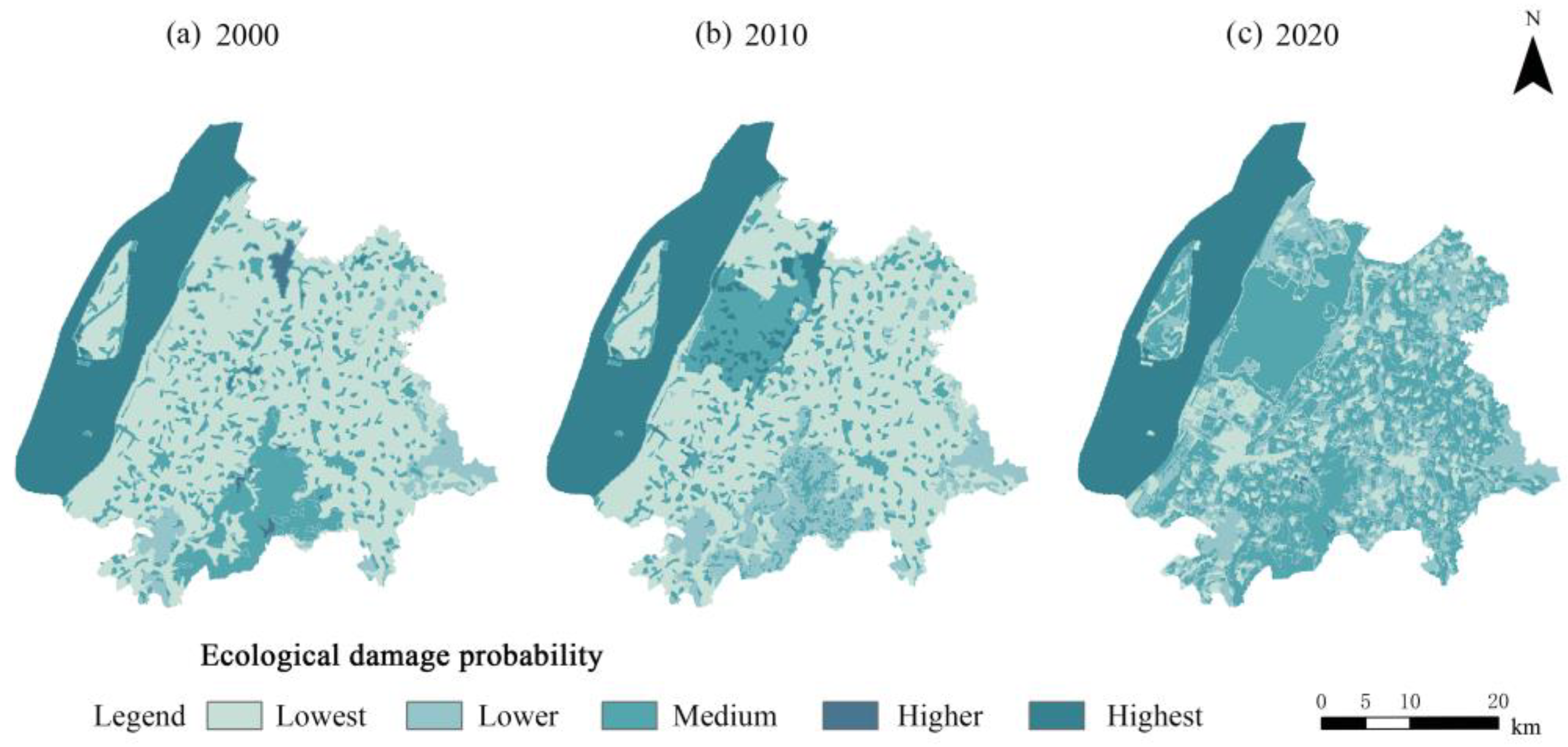
3.2.2. Evolution of Ecological Degradation Probability in Rural Landscapes

The ecological damage driving factors for the three periods in the study area were normalized. From the perspective of individual ecological damage driving factors (Figure 6), the area of impermeable surfaces has steadily increased, expanding rapidly from 2010 to 2020, mainly concentrated near densely construction areas in the northwest, with a large permeable surface in the west due to the Yangtze River water body; road density gradually increased, with rural settlements mostly located near major transportation corridors such as (G4211), Nanjing Third Ring (S002), and Ningwu Avenue (G205); vegetation coverage in the west was lower, and due to recent human activities, the increase in construction land led to habitat fragmentation and pollution; ecological land connectivity in the west and south was relatively high with little change, mainly concentrated in areas with water bodies and forest land; in contrast, the connectivity of construction land significantly changed between 2000 and 2010, focusing on the central and western parts; the landscape vulnerability of water bodies and cultivated land was higher than that of the central and southern areas, with the vulnerability of cultivated land noticeably increasing by 2020.
By combining the results of the individual factor assessments and using the natural breaks method, the rural landscape ecological damage probability was classified into five levels: lowest ecological damage probability (0 < PROB ≤ 0.1151), lower ecological damage probability (0.1151 < PROB ≤ 0.2372), medium ecological damage probability (0.2372 < PROB ≤ 0.3566), higher ecological damage probability (0.3566 < PROB ≤ 0.4548), and highest ecological damage probability (PROB > 0.4548). The ecological damage probability for the other years was classified based on the standard set in 2000 (Figure 7). Overall, the landscape damage probability continued to rise, with the lowest-, lower-, and medium-damage probability zones predominating. Over the 20 years, the areas with the lowest, lower, and highest damage probabilities decreased, and were mostly composed of cultivated land and forest land; the medium-damage-probability areas significantly increased, mainly concentrated in the centrally construction regions such as Xinzhu Village and Jiangning Community; the highest-damage-probability areas showed minimal change, continuing to be distributed around water sources in the western region.

3.2.3. Evolution of Ecological Risk in Rural Landscapes

Based on the rural LERA formula (1), the landscape ecological value and ecological damage probability in the study area were calculated using raster computation in ArcGIS 10.8, resulting in the rural LERA index for three periods. To facilitate the comparison of landscape ecological risk changes across different periods, and based on the regional actual conditions and previous related studies [20], the LER in 2000 was classified into five levels. The classification for 2010 and 2020 was based on the 2000 standard (Figure 8): lowest-risk areas (0 < RISK ≤ 5 × 10⁵ CNY/ha), lower-risk areas (5 × 10⁵ < RISK ≤ 450 × 105 CNY/ha), medium-risk areas (450 × 105 < RISK ≤ 650×105 CNY/ha), higher-risk areas (650 × 105 < RISK ≤ 1000 × 105 CNY/ha), and highest-risk areas (RISK ≥ 1000 × 105 CNY/ha).
Over the past 20 years, the area of lowest ecological risk zones has increased, primarily due to the development of construction land, especially in areas such as Jiangning and Shengjiang communities, with an increase of 25.58 km2. The area of lower ecological risk zones has continued to decrease, with much of the original cultivated land converted to medium- and higher-risk areas. The area of medium-ecological-risk zones has steadily increased, primarily distributed in cultivated land areas. From 2000 to 2020, the area classified as higher ecological risk increased by a net amount of 46.67 km2. In 2020, the higher-ecological-risk zones accounted for 20.57% of the total area, primarily consisting of scattered and fragmented cultivated land, except for the more contiguous forest land in the south. The area of highest-ecological-risk zones has shown little change, primarily distributed along the Yangtze River in the west and around water bodies within the villages.

3.3. Spatial Autocorrelation Analysis of Rural Landscape Ecological Risk

3.3.1. Global Spatial Clustering Characteristics

Using the GeoDa platform, spatial weight matrices were constructed, and the Moran’s I-values for the years 2000, 2010, and 2020 were calculated as 0.920, 0.914, and 0.938, respectively. All values are greater than 0, with p-values less than 0.001 (Figure 9), indicating a highly significant positive spatial autocorrelation of rural LER. This suggests that the distribution of ecological risk exhibits strong spatial clustering.

3.3.2. Identification of Local Spatial Clustering Patterns

Local spatial autocorrelation analysis further revealed the spatial clustering characteristics and localized distribution patterns of rural LER within the study area (Figure 10). The results indicate that ecological risks predominantly exhibit High-High and Low-Low clustering types. From 2000 to 2020, High-High clusters were mainly concentrated along the western riverside areas and in water-adjacent villages such as Xintong, Sijia, and Shengjiang. These areas, subject to both anthropogenic disturbance and natural stressors, remained ecologically vulnerable and consistently exhibited high levels of risk. In contrast, Low-Low clusters were concentrated in the southeastern regions of Hongmu and Xining, which are rich in forest and cultivated land resources, indicating low risk levels and strong spatial stability. By 2010, the spatial extent of Low-Low clusters reached its peak. However, due to intensified agricultural and construction activities in subsequent years, the degree of spatial clustering declined, and some areas transitioned into non-significant or marginal clusters. Low-High outliers, primarily located at the periphery of High-High clusters, suggest a potential outward expansion of high-risk zones, highlighting the need for early intervention to prevent ecological risk spillover. High-Low outliers were sparsely distributed along the edges of low-risk regions. By 2020, their number had significantly decreased, with most becoming non-significant or merging into Low-Low clusters. This shift indicates that localized high-risk points were absorbed or mitigated by surrounding ecosystems, leading to a more balanced ecological structure. Such changes may be attributed to reduced development intensity, ecological restoration efforts, or optimized land use, reflecting a gradual weakening of ecological disturbance boundaries and a decline in spatial autocorrelation.

3.4. Driving Factors Analysis of Rural Landscape Ecological Risk

According to the results of the factor detector (Table 6), all six driving factors have a certain impact on the spatial distribution of rural LER, with all p-values being less than 0.001, indicating statistical significance. In 2000, the explanatory power (q-values) of the factors ranked as follows: landscape vulnerability > vegetation coverage > ecological land connectivity > distance to road > impervious surface ratio > construction land connectivity. This ranking remained largely unchanged in 2010; however, the explanatory power of distance to road—an external factor reflecting the intensity of human disturbance—continued to increase and became the second-most influential factor by 2020. This indicates a growing influence of human activities on regional ecological risks. Overall, landscape vulnerability, ecological land connectivity, and vegetation coverage were the dominant drivers determining the stability and sensitivity of rural ecosystems. Meanwhile, distance to road, as a proxy for spatial expansion and land development pressure, has become increasingly influential in recent years, reflecting a trend of rising ecological risk in urban–rural transition zones. Although the impervious surface ratio and construction land connectivity showed relatively low individual explanatory power, they still contributed to the formation of localized ecological risks.
According to the results of interaction detection (Figure 11), from 2000 to 2020, the interaction q-values of any two factors were higher than those of the corresponding individual factors, indicating overall nonlinear enhancement or bivariate enhancement. The continuous increase in q-values across the three periods suggests that the formation of ecological risk is significantly driven by compound interactions. In 2000, the interaction between ecological land connectivity and landscape fragility had the highest explanatory power (q = 0.9788), followed by vegetation coverage ∩ landscape fragility (q = 0.9408) and impervious surface ratio ∩ landscape fragility (q = 0.9310). This highlights the strong coupling effects among ecological structural factors, and suggests that the combined influence of early human disturbance and ecological fragility may have led to local risk amplification, providing an important basis for identifying and forecasting high-risk potential areas. In 2010, the overall interaction relationships among the factors remained strong. The interaction between ecological land connectivity and landscape fragility continued to be the most dominant (q = 0.9770). Meanwhile, combinations such as impervious surface ratio ∩ construction land connectivity, distance to road ∩ impervious surface ratio, and ecological land connectivity ∩ distance to road showed increased explanatory power, indicating the emergence of interference effects between spatial development pressure and ecological structure, and the gradual formation of a compound risk pattern in urban–rural fringe areas. By 2020, the combinations with the highest explanatory power remained consistent with those in 2000 and 2010. Although impervious surface ratio, construction land connectivity, and distance to road still exhibited relatively low individual explanatory power, the findings reflect a continued increase in the penetration effect of construction activities on ecosystems, suggesting a tendency toward spatial risk amplification.

4. Discussion

4.1. Changes in Rural Landscape Types

The land use changes reflect an ongoing tension between urban expansion and ecological conservation [49]. The landscape is primarily composed of cultivated land, construction land, and water bodies. Over the past 20 years, urbanization has significantly impacted rural areas, with cultivated land sharply declining due to the expansion of construction land. Although the rate of loss slowed after 2010, it continues to pose risks to food security and ecological stability. The increase in construction land mainly resulted from the conversion of cultivated and unused land. The establishment of the Binjiang Economic Development Zone in 2003 further accelerated development in the northwest of the study area. Forest and grassland areas declined slightly, indicating that ecological protection policies have played a role in limiting development intensity. The expansion of water bodies is closely linked to initiatives such as the “sponge city” program, river regulation, and reservoir projects, all of which have contributed to enhancing regional ecological resilience.

4.2. Spatiotemporal Assessment of Rural Landscape Ecological Risk

The assessment results indicate that the overall LER exhibited an upward trend from 2000 to 2020. The lowest- and lower-ecological-risk areas were primarily distributed in the transitional zones between rural settlements and farmland, closely aligning with the spatial distribution of construction land. Despite a certain level of anthropogenic disturbance, since 2010, particularly around Xinzhou Village, the boundaries of construction land have stabilized and become more concentrated, leading to a reduction in LER, which is consistent with the findings of Peng et al. [50]. Medium- and higher-risk areas continued to expand, with medium-risk zones mainly concentrated in cultivated land. The expansion of construction land disrupted the connectivity of farmland landscapes, reducing ecosystem stability and elevating ecological risk, aligning with the conclusions of He et al. [51]. Higher-risk areas are mostly forest land. Due to their strong ecological sensitivity, the risks they face when exposed to the same external disturbances are higher than those of construction land, which verifies the viewpoint of Yu et al. [52]. The highest-risk areas were largely concentrated near the Yangtze River in the western part of the study area, which is consistent with the research results of Huang et al. [53] on the green spaces in the water network area of southern Jiangsu. The water area itself has a higher ecological value and is also an area with frequent human activities. Therefore, its comprehensive ecological risk level is significantly high. In terms of driving factors, natural ecological variables dominated regional ecological carrying capacity. Adili et al. [54] found that natural variables such as NDVI and DEM had stronger explanatory power for ecological risks than socioeconomic factors in the Ebinur Lake Basin. This aligns closely with our findings that landscape structure variables, such as landscape vulnerability and vegetation connectivity, play a leading role in ecological risk regulation. In contrast, among anthropogenic factors, the influence of “distance to road” increased steadily and had become a secondary dominant factor by 2020, indicating growing ecological pressure driven by urban expansion in peri-urban areas. Although the explanatory power of the impervious surface ratio was limited when considered independently, it showed significant synergistic effects in interaction detection, revealing a trend of localized risk amplification.
Compared to existing LERA studies, classification outcomes may differ due to varying evaluation perspectives and functional weight assignments. For example, Li et al. [55] found that coastal mudflats and marine areas in Zhoushan exhibited higher ecological risks, which is consistent with our results. In contrast, Pan et al. [56] emphasized the ecological buffering capacity of water bodies and classified them as lower-risk areas. In our study, given the high intensity of human activities in Jiangning District, water bodies were categorized as high-risk areas, reflecting the ability to identify zones with “high ecological value but high disturbance pressure”. Additionally, topographic factors such as elevation and slope were found to significantly influence spatial patterns of ecological risk. Yan et al. [57] observed that LER exhibits regular variation across different terrain gradients. Future research should further refine indicator systems and classification criteria based on regional ecological functions and anthropogenic activity contexts to enhance the adaptability and practical value of ecological risk assessments.

4.3. Planning Strategies

Based on the LERA of the study area, and in reference to policy documents such as the Nanjing “14th Five-Year” Ecological and Environmental Protection Plan and the Nanjing Jiangning District Territorial Spatial Master Plan (2021–2035) [58,59], the study area is divided into three ecological regulation zones according to topographic characteristics, area distribution, and land use types, with corresponding planning strategies proposed for each zone.
(1)
Ecological Conservation Zone: This zone corresponds to areas with the highest rural LER, accounting for 17.13% of the study area. It is primarily concentrated along the strip-shaped water bodies in the western region and small fragmented patches surrounding rivers within the villages. According to the results of driving factor detection, although ecological land connectivity is relatively good in these areas, the ecosystems are highly sensitive due to high landscape vulnerability and strong external pressures such as proximity to roads and intensive development disturbance. These areas should be prioritized within the ecological protection redline and subject to strict control of human disturbances. It is recommended to focus on the implementation of water buffer zone construction, ecological water-saving measures, and restrictions on construction activities to enhance ecosystem stability [60]. In particular, riverside communities such as Xintong, Sijia, and Shengjiang should establish strict environmental monitoring stations to conduct long-term tracking of water quality, biodiversity, and soil safety, forming an early warning mechanism [61]. Meanwhile, low-impact economic activities such as ecological agriculture and ecotourism should be encouraged to integrate ecological protection with economic development, promoting a sustainable feature.
(2)
Ecological Restoration Zone: This zone corresponds to areas with medium- to higher-LER, accounting for 56.07% of the total study area. These areas are mostly contiguous patches dominated by cultivated land, forestland, and grassland, with relatively high vegetation coverage. However, with the significant impact of human activities, especially between 2010 and 2020, a large amount of farmland has shifted from medium-risk to higher-risk. Driving factor analysis indicates that local ecological land connectivity has been disrupted, and areas near roads experience frequent human activities and significant declines in vegetation cover. It is therefore necessary to prohibit or strictly regulate irregular land reclamation and construction activities to prevent the conversion of farmland into construction land. Given the high ecological potential of this zone, ecological engineering techniques—such as farmland water networks, vegetative erosion control belts, and interception ditches—should be introduced to improve rural ecosystem structure and enhance connectivity among ecological lands [62]. While reducing LER, efforts should also focus on improving economic benefits. Wen et al. [63] pointed out in their study of the land ecosystems in the Guangdong–Hong Kong–Macao Greater Bay Area that ecological protection and economic development are not mutually exclusive: by enhancing ecosystem quality and optimizing spatial patterns, a win-win outcome can be achieved. For instance, in Xining Village in the southern part of the study area, there are vast stretches of cypress and bamboo forests, surrounded by mountains and water, and it has excellent resources for fruit tree and tea cultivation. It is possible to develop a characteristic forest and fruit economy and promote the development of homestay and eco-tourism industries. In the southeast, Hongmu Village was designated a national forest village in 2019 [64], boasting significant forest and cultivated land, as well as high-quality planting resources. The village should leverage its ecological strengths to promote a development model that integrates “specialized planting + ecotourism”, thus transforming ecological advantages into economic gains [65].
(3)
Ecological Enhancement Zone: This zone corresponds to areas with the lower and lowest levels of LER, accounting for 26.79% of the total study area. These zones are distributed in patchy and planar patterns around cultivated land, villages, and other construction land. They exhibit high connectivity of construction land and possess substantial development potential. However, ecological concerns such as a high proportion of impervious surfaces and insufficient green coverage also exist, necessitating ecological interventions to strengthen system resilience. The area has an advanced manufacturing base. It is recommended to adopt a development model of “moderate development + integration of green infrastructure” with strict control over high pollution and high energy consuming industries. Instead, low-impact industries such as cultural and creative sectors and green manufacturing should be encouraged. In areas with a high proportion of impervious surfaces, the introduction of eco-friendly infrastructure such as permeable pavements and constructed wetlands is advised to reduce stormwater runoff and promote groundwater recharge. In villages with low vegetation cover, strict ecological protection boundaries should be implemented, along with rational spatial planning for production, living, and ecological functions. Additionally, efforts should be made to develop cultural tourism brands by preserving and promoting historical architectural heritage, thereby fostering a synergistic development model of “ecology + culture + tourism”.

4.4. Limitations and Improvements

Although this study establishes a LERA framework suitable for peri-urban villages, certain limitations remain. First, in terms of data precision, the study primarily relies on medium-resolution remote sensing imagery for land use classification and index calculation. Future research could benefit from incorporating high-resolution remote sensing and ground-based monitoring data to improve accuracy. Second, the model is constructed based on the natural and socioeconomic characteristics of villages in Jiangning District, and its applicability to areas with more complex ecological patterns and distinct disturbance mechanisms requires further validation. Comparative studies across diverse regions and village types are recommended to enhance the model’s generalizability and transferability. Third, this study adopts the equivalence factor method for estimating ESV due to its simplicity, wide application, and regional adaptability. However, despite adjustments made to the equivalence coefficients based on local ecological and socioeconomic conditions, the calibration process still involves a degree of subjectivity. As a result, uncertainty may be introduced into the magnitude and spatial patterns of ESV estimation. To address these limitations, future studies are encouraged to incorporate empirically derived, locally calibrated correction factors to enhance the robustness and credibility of ESV assessments. Finally, landscape ecology theories can be more systematically integrated into the LERA process. For instance, constructing an evaluation framework based on the triad of “heterogeneity–connectivity–stability” may offer a more scientific understanding of how landscape pattern changes affect ESs. Moreover, the current assessment results are insufficiently linked with policy instruments. Future research should strengthen the synergy between LER evaluation outcomes and institutional tools such as spatial planning, ecological redlines, and compensation mechanisms to improve policy implementation effectiveness. To enhance the empirical basis and application value of the model, multi-source data such as field investigations, questionnaire surveys, and drone images can also be introduced for verification.

5. Conclusions

This study takes the rural areas of Jiangning District, Nanjing as the research object and constructs a dual-dimensional coupling model integrating ESV and ecological risk probability to systematically assess the spatiotemporal evolution of rural LER from 2000 to 2020 and explore its main driving mechanisms. The main conclusions are as follows:
(1)
Significant changes occurred in land use patterns. Construction land expanded substantially, while cultivated land continued to decline, reflecting a trend of land resource restructuring driven by urbanization. Water bodies slightly increased, and forest and grassland areas remained generally stable.
(2)
The overall ESV increased. Regulating services dominated, accounting for more than 82% of the total ESV. High-value areas were concentrated around water bodies in the northwest and forested areas in the south. Cultivated and forest land continued to play a core role in supporting and provisioning services. Although cultural services accounted for a smaller share, they showed potential for enhancement in specific areas.
(3)
LER continued to rise, with spatial distribution becoming more concentrated. The area of medium- to highest-risk zones expanded significantly, showing a tendency to cluster toward urban edges and the northwestern area with high construction intensity. Structural factors were the main drivers of rural LER, and interaction effects were notable. Landscape vulnerability, vegetation coverage, and ecological land connectivity were the core influencing factors, while the impact of distance to road increased steadily. The interaction among ecological structural factors had a significant amplifying effect on high-risk zones.
(4)
Based on the evolution of risk patterns and their driving mechanisms, the study delineates three functional zones: the ecological conservation zone, ecological restoration zone, and ecological enhancement zone. This zoning provides scientific support for improving the precision of rural spatial governance and promoting sustainable development.

Author Contributions

Conceptualization, Y.X., Y.L. and Y.Y.; methodology, Y.X., Y.L. and Y.Y.; software, Y.L. and Y.X.; validation, Y.X., Y.L. and Y.Y.; formal analysis, Y.X. and Y.Y.; investigation, Y.L.; resources, Y.X. and Y.Y.; data curation, Y.X. and Y.L.; writing—original draft preparation, Y.L.; writing—review and editing, Y.X., Y.L. and Y.Y.; visualization, Y.L.; supervision, Y.X. and Y.Y.; project administration, Y.X. and Y.Y.; funding acquisition, Y.X. and Y.Y. All authors have read and agreed to the published version of the manuscript.

Funding

This research was funded by the National Natural Science Foundation of China (Grant No. 32171859), the Humanities and Social Science Research Project of the Ministry of Education (Grant No. 21YJCZH187), and the Qing Lan Project, the Postgraduate Research & Practice Innovation Program of Jiangsu Province (Grant No. KYCX24_1335).

Institutional Review Board Statement

Not applicable.

Informed Consent Statement

Not applicable.

Data Availability Statement

The data used in this study can be requested from the authors.

Conflicts of Interest

The authors declare no conflicts of interest.

References

  1. Liu, Y.; Zang, Y.; Yang, Y. China’s rural revitalization and development: Theory, technology and management. J. Geogr. Sci. 2020, 30, 1923–1942. [Google Scholar] [CrossRef]
  2. da Silva, R.F.; Rodrigues, M.D.; Vieira, S.; Batistella, M.; Farinaci, J. Perspectives for environmental conservation and ecosystem services on coupled rural-urban systems. Perspect. Ecol. Conserv. 2017, 15, 74–81. [Google Scholar] [CrossRef]
  3. Zhang, Q.; Wang, J. Multi-functional coupling-based rural ecological pattern construction and network prioritization evaluation: A case study of Jiangning District, Nanjing. Ecol. Indic. 2024, 166, 112277. [Google Scholar] [CrossRef]
  4. Zhang, Y.; Li, Y.; Lv, J.; Wang, J.; Wu, Y. Scenario simulation of ecological risk based on land use/cover change-A case study of the Jinghe county, China. Ecol. Indic. 2021, 131, 108176. [Google Scholar] [CrossRef]
  5. Ji, X.; Wu, D.; Yan, Y.; Guo, W.; Li, K. Interpreting regional ecological security from perspective of ecological networks: A case study in Ningxia Hui Autonomous Region, China. Environ. Sci. Pollut. Res. 2023, 30, 65412–65426. [Google Scholar] [CrossRef]
  6. Zhao, W.; Jiang, C. Analysis of the Spatial and Temporal Characteristics and Dynamic Effects of Urban-Rural Integration Development in the Yangtze River Delta Region. Land 2022, 11, 1054. [Google Scholar] [CrossRef]
  7. Mamut, A.; Eziz, M.; Mohammad, A.; Anayit, M. The spatial distribution, contamination, and ecological risk assessment of heavy metals of farmland soils in Karashahar-Baghrash oasis, northwest China. Hum. Ecol. Risk Assess. 2017, 23, 1300–1314. [Google Scholar] [CrossRef]
  8. Li, X.; Li, S.; Zhang, Y.; O’Connor, P.; Zhang, L.; Yan, J. Landscape Ecological Risk Assessment under Multiple Indicators. Land 2021, 10, 739. [Google Scholar] [CrossRef]
  9. Lin, D.; Liu, F.; Zhang, J.; Hao, H.; Zhang, Q. Research progress on ecological risk assessment based on multifunctional landscape. J. Resour. Ecol. 2021, 12, 260–267. [Google Scholar] [CrossRef]
  10. Xiong, X.; Tang, X.; Liu, L.; Wang, J. Traditional rural landscape security pattern construction based on” Source-Sink” theory. J. Nanjing For. Univ. 2019, 43, 143–151. [Google Scholar] [CrossRef]
  11. Wang, S.; Zhao, Y.; Ren, H.; Zhu, S.; Yang, Y. Identification of Ecological Risk “Source-Sink” Landscape Functions of Resource-Based Region: A Case Study in Liaoning Province, China. Land 2023, 12, 1921. [Google Scholar] [CrossRef]
  12. Yang, Y.; Chen, J.; Lan, Y.; Zhou, G.; You, H.; Han, X.; Wang, Y.; Shi, X. Landscape Pattern and Ecological Risk Assessment in Guangxi Based on Land Use Change. Int. J. Environ. Res. Public Health 2022, 19, 1595. [Google Scholar] [CrossRef]
  13. Li, S.; He, W.; Wang, L.; Zhang, Z.; Chen, X.; Lei, T.; Wang, S.; Wang, Z. Optimization of landscape pattern in China Luojiang Xiaoxi basin based on landscape ecological risk assessment. Ecol. Indic. 2023, 146, 109887. [Google Scholar] [CrossRef]
  14. Xie, J.; Zhao, J.; Zhang, S.; Sun, Z. Optimal Scale and Scenario Simulation Analysis of Landscape Ecological Risk Assessment in the Shiyang River Basin. Sustainability 2023, 15, 15883. [Google Scholar] [CrossRef]
  15. Zhan, D.; Quan, B.; Liao, J. The Spatiotemporal Evolution and Coupling Coordination of LUCC and Landscape Ecological Risk in Ecologically Vulnerable Areas: A Case Study of the Wanzhou-Dazhou-Kaizhou Region. Sustainability 2025, 17, 4399. [Google Scholar] [CrossRef]
  16. Wang, H.; Liu, X.; Zhao, C.; Chang, Y.; Liu, Y.; Zang, F. Spatial-temporal pattern analysis of landscape ecological risk assessment based on land use/land cover change in Baishuijiang National nature reserve in Gansu Province, China. Ecol. Indic. 2021, 124, 107454. [Google Scholar] [CrossRef]
  17. Kang, L.; Yang, X.; Gao, X.; Zhang, J.; Zhou, J.; Hu, Y.; Chi, H. Landscape ecological risk evaluation and prediction under a wetland conservation scenario in the Sanjiang Plain based on land use/cover change. Ecol. Indic. 2024, 162, 112053. [Google Scholar] [CrossRef]
  18. Xu, W.; Wang, J.; Zhang, M.; Li, S. Construction of landscape ecological network based on landscape ecological risk assessment in a large-scale opencast coal mine area. J. Clean. Prod. 2021, 286, 125523. [Google Scholar] [CrossRef]
  19. Cao, Q.; Zhang, X.; Ma, H.; Wu, J. Review of landscape ecological risk and an assessment framework based on ecological services: ESRISK. Acta Geogr. Sin. 2018, 73, 843–855. [Google Scholar] [CrossRef]
  20. Hu, Y.; Gao, G. Framework and practice of urban landscape ecological risk assessment: A case study of the Tiantan Region in Beijing. Acta Ecol. Sin. 2020, 40, 7805–7815. [Google Scholar] [CrossRef]
  21. Tang, L.; Long, H.; Aldrich, D.P. Putting a Price on Nature: Ecosystem Service Value and Ecological Risk in the Dongting Lake Area, China. Int. J. Environ. Res. Public Health 2023, 20, 4649. [Google Scholar] [CrossRef]
  22. Zhou, X.; Ji, G.; Wang, F.; Ji, X. Identification and simulation of ecological zoning in the Yangtze River Delta (YRD) urban agglomeration based on Ecological Service Value (ESV)- Landscape Ecological Risk (LER). J. Clean. Prod. 2025, 516, 145778. [Google Scholar] [CrossRef]
  23. Ji, X.; Sun, Y.; Guo, W.; Zhao, C.; Li, K. Land use and habitat quality change in the Yellow River Basin: A perspective with different CMIP6-based scenarios and multiple scales. J. Environ. Manag. 2023, 345, 118729. [Google Scholar] [CrossRef]
  24. Hu, G.; Guo, Y.; Zhang, C.; Chen, Y.; Lang, Y.; Su, L.; Huang, H. Landscape ecological risk assessment of the northern coastal region of China based on the improved ESRISK framework: A case study of Cangzhou City. Ecol. Indic. 2025, 171, 113222. [Google Scholar] [CrossRef]
  25. Lin, X.; Wang, Z. Landscape ecological risk assessment and its driving factors of multi-mountainous city. Ecol. Indic. 2023, 146, 109823. [Google Scholar] [CrossRef]
  26. Liu, R.; Zhang, L.; Tang, Y.; Jiang, Y. Understanding and evaluating the resilience of rural human settlements with a social-ecological system framework: The case of Chongqing Municipality, China. Land Use Policy 2024, 136, 106966. [Google Scholar] [CrossRef]
  27. Wang, H.; Qin, F.; Xu, C.; Li, B.; Guo, L.; Wang, Z. Evaluating the suitability of urban development land with a Geodetector. Ecol. Indic. 2021, 123, 107339. [Google Scholar] [CrossRef]
  28. Xu, X.; Liu, J.; Zhang, S.; Li, R.; Yan, C.; Wu, S. China’s Multi-Period Land Use Land Cover Remote Sensing Monitoring Data Set (CNLUCC); Resource and Environment Data Cloud Platform: Beijing, China, 2018. [Google Scholar] [CrossRef]
  29. Karimian, H.; Zou, W.; Chen, Y.; Xia, J.; Wang, Z. Landscape ecological risk assessment and driving factor analysis in Dongjiang river watershed. Chemosphere 2022, 307, 135835. [Google Scholar] [CrossRef]
  30. Huang, L.; Yuan, L.; Xia, Y.; Yang, Z.; Luo, Z.; Yan, Z.; Li, M.; Yuan, J. Landscape ecological risk analysis of subtropical vulnerable mountainous areas from a spatiotemporal perspective: Insights from the Nanling Mountains of China. Ecol. Indic. 2023, 154, 110883. [Google Scholar] [CrossRef]
  31. Sui, L.; Yan, Z.; Li, K.; Wang, C.; Shi, Y.; Du, Y. Prediction of ecological security network in Northeast China based on landscape ecological risk. Ecol. Indic. 2024, 160, 111783. [Google Scholar] [CrossRef]
  32. Guan, D.; Cao, J.; Huang, D.; Zhou, L. Early warning level identification and evolutionary trend prediction of ecological risk in the upper Chang Jiang (Yangtze, R.), China. Front. Earth Sci. 2025, 19, 149–167. [Google Scholar] [CrossRef]
  33. Jiang, Z.; Gan, X.; Liu, J.; Bi, X.; Kang, A.; Zhou, B. Landscape Ecological Risk Assessment and Zoning Control Based on Ecosystem Service Value: Taking Sichuan Province as an Example. Appl. Sci. 2023, 13, 12103. [Google Scholar] [CrossRef]
  34. Assessment, M.E. Millennium ecosystem assessment. In Ecosystems and Human Wellbeing: A Framework for Assessment; World Resources Institute: Washington, DC, USA, 2005; p. 51. [Google Scholar]
  35. Costanza, R.; d’Arge, R.; De Groot, R.; Farber, S.; Grasso, M.; Hannon, B.; Limburg, K.; Naeem, S.; O’neill, R.V.; Paruelo, J. The value of the world’s ecosystem services and natural capital. Nature 1997, 387, 253–260. [Google Scholar] [CrossRef]
  36. Xie, G.; Zhang, C.; Zhang, L.; Chen, W.; Li, S. Improvement of the evaluation method for ecosystem service value based on per unit area. J. Nat. Resour. 2015, 30, 1243–1254. [Google Scholar] [CrossRef]
  37. Li, F.; Wang, F.; Liu, H.; Huang, K.; Yu, Y.; Huang, B. A comparative analysis of ecosystem service valuation methods: Taking Beijing, China as a case. Ecol. Indic. 2023, 154, 110872. [Google Scholar] [CrossRef]
  38. Sun, C.; Gu, B.; Zhang, J. Ecosystem service value assessment based on clustering analysis and ESV algorithm. World Sci. Res. J. 2020, 6, 54–61. [Google Scholar] [CrossRef]
  39. Du, J.; Shrestha, R.P.; Nitivattananon, V.; Nguyen, T.P.; Razzaq, A. Unveiling the value of nature: A comprehensive analysis of the ecosystem services and ecological compensation in Wuhan city’s urban lake wetlands. Water 2023, 15, 2257. [Google Scholar] [CrossRef]
  40. Zandebasiri, M.; Jahanbazi Goujani, H.; Iranmanesh, Y.; Azadi, H.; Viira, A.-H.; Habibi, M. Ecosystem services valuation: A review of concepts, systems, new issues, and considerations about pollution in ecosystem services. Environ. Sci. Pollut. Res. 2023, 30, 83051–83070. [Google Scholar] [CrossRef]
  41. Wang, J.; Zhang, Y.; Xia, L.; Li, J.; He, H.; Liu, S. Soil conservation and water conservation services and trade-offs following the land consolidation project: A case study of Yan’an city, China. Front. Environ. Sci. 2024, 12, 1425199. [Google Scholar] [CrossRef]
  42. Lu, Z.; Song, Q.; Zhao, J.; Wang, S. Prediction and evaluation of ecosystem service value based on land use of the Yellow River source area. Sustainability 2022, 15, 687. [Google Scholar] [CrossRef]
  43. Shen, M.; Hang, Z.; Liu, Y.; Chen, J.; Yin, Z. Spatio-temporal changes of ecological service value based on improved equivalent factor method: Case study on yangtze River Basin. J. Changjiang River Sci. Res. Inst. 2023, 40, 47. [Google Scholar]
  44. Ghosh, A.; Maiti, R. Development of new Ecological Susceptibility Index (ESI) for monitoring ecological risk of river corridor using F-AHP and AHP and its application on the Mayurakshi river of Eastern India. Ecol. Inform. 2021, 63, 101318. [Google Scholar] [CrossRef]
  45. Li, L.; Tang, H.; Lei, J.; Song, X. Spatial autocorrelation in land use type and ecosystem service value in Hainan Tropical Rain Forest National Park. Ecol. Indic. 2022, 137, 108727. [Google Scholar] [CrossRef]
  46. Yang, J.; Liu, Q.; Deng, M. Spatial hotspot detection in the presence of global spatial autocorrelation. Int. J. Geogr. Inf. Sci. 2023, 37, 1787–1817. [Google Scholar] [CrossRef]
  47. Song, Y.; Wang, J.; Ge, Y.; Xu, C. An optimal parameters-based geographical detector model enhances geographic characteristics of explanatory variables for spatial heterogeneity analysis: Cases with different types of spatial data. GISci. Remote Sens. 2020, 57, 593–610. [Google Scholar] [CrossRef]
  48. Hua, D.; Hao, X. Spatiotemporal change and drivers analysis of desertification in the arid region of northwest China based on geographic detector. Environ. Chall. 2021, 4, 100082. [Google Scholar]
  49. Cao, X.; Liu, Z.; Li, S.; Gao, Z. Integrating the ecological security pattern and the PLUS model to assess the effects of regional ecological restoration: A case study of Hefei City, Anhui Province. Int. J. Environ. Res. Public Health 2022, 19, 6640. [Google Scholar] [CrossRef]
  50. Peng, J.; Xie, P.; Liu, Y.; Hu, X. Integrated ecological risk assessment and spatial development trade-offs in low-slope hilly land: A case study in Dali Bai Autonomous Prefecture, China. Acta Geogr. Sin. 2015, 70, 1747–1761. [Google Scholar] [CrossRef]
  51. Gao, H.; Song, W. Assessing the landscape ecological risks of land-use change. Int. J. Environ. Res. Public Health 2022, 19, 13945. [Google Scholar] [CrossRef]
  52. Yu, Y.; Cui, W.; Liu, S.; Yu, T.; Song, Y. Evolutionary analysis of landscape ecological risk in Baili Rhododendron National Forest Park. PLoS ONE 2025, 20, e0317851. [Google Scholar] [CrossRef]
  53. Huang, X.; Ding, J.; Wang, D. Spatiotemporal evolution and regulation strategies of ecological risks in green space landscape in the water network area of southern Jiangsu. Zhejiang Agric. For. Univ. 2024, 41, 1283–1292. [Google Scholar] [CrossRef]
  54. Adili, A.; Wu, B.; Chen, J.; Wu, N.; Ge, Y.; Abuduwaili, J. Assessment of Landscape Ecological Risk and Its Driving Factors for the Ebinur Lake Basin from 1985 to 2022. Land 2024, 13, 1572. [Google Scholar] [CrossRef]
  55. Li, S.; Wang, L.; Zhao, S.; Gui, F.; Le, Q. Landscape ecological risk assessment of Zhoushan Island based on LULC change. Sustainability 2023, 15, 9507. [Google Scholar] [CrossRef]
  56. Pan, J.; Li, B. Simulation and analysis of human dimensions of urban thermal environment in valley-city: A case study of Lanzhou City. Arid Land Geogr. 2011, 34, 662–670. [Google Scholar]
  57. Yan, J.; Qiao, H.; Li, Q.; Song, M.; Yao, X.; Gao, P.; Zhang, M.; Li, J.; Qi, G.; Li, G. Landscape ecological risk assessment across different terrain gradients in the Yellow River Basin. Front. Environ. Sci. 2024, 11, 1305282. [Google Scholar] [CrossRef]
  58. Nanjing Municipal Bureau of Ecology and Environment. The 14th Five-Year Plan for Ecological and Environmental Protection of Nanjing. 2022. Available online: https://sthjj.nanjing.gov.cn/njshjbhj/202202/t20220209_3285947.html (accessed on 17 March 2025).
  59. People’s Government of Jiangning District, Nanjing. Territorial Spatial Master Plan of Jiangning District, Nanjing (2021–2035). 2025. Available online: http://www.jiangning.gov.cn/xwzx/gzdt/202503/t20250325_5102628.html (accessed on 29 March 2025).
  60. Yang, F.; Xiong, S.; Ou, J.; Zhao, Z.; Lei, T. Human settlement resilience zoning and optimizing strategies for river-network cities under flood risk management objectives: Taking Yueyang City as an example. Sustainability 2022, 14, 9595. [Google Scholar] [CrossRef]
  61. Bao, T.; Wang, R.; Song, L.; Liu, X.; Zhong, S.; Liu, J.; Yu, K.; Wang, F. Spatio-temporal multi-scale analysis of landscape ecological risk in Minjiang River Basin based on adaptive cycle. Remote Sens. 2022, 14, 5540. [Google Scholar] [CrossRef]
  62. Dollinger, J.; Dagès, C.; Bailly, J.-S.; Lagacherie, P.; Voltz, M. Managing ditches for agroecological engineering of landscape. Agron. Sustain. Dev. 2015, 35, 999–1020. [Google Scholar] [CrossRef]
  63. Wen, Y.; Yang, J.; Liao, W.; Xiao, J.; Yan, S. Refined assessment of space-time changes, influencing factors and socio-economic impacts of the terrestrial ecosystem quality: A case study of the GBA. J. Environ. Manag. 2023, 345, 118869. [Google Scholar] [CrossRef]
  64. National Forestry and Grassland Administration. The Notice of the National Forestry and Grassland Administration Announced About the First Batch of National Forest Villages. Available online: https://www.forestry.gov.cn/hjhb/4994/20200117/181717325474987.html (accessed on 23 February 2025).
  65. Gao, H.; Ouyang, Z.; Zheng, H.; Bluemling, B. Perception and attitudes of local people concerning ecosystem services of culturally protected forests. Acta Ecol. Sin. 2013, 33, 756–763. [Google Scholar] [CrossRef]
Figure 1. The research framework in the study.
Sustainability 17 07014 g001
Figure 2. Location of the study area.
Sustainability 17 07014 g002
Figure 3. Sankey diagram of regional land use transfer from 2000 to 2020.
Sustainability 17 07014 g003
Figure 4. (a) Changes in ESV of different land use types in the study area from 2000 to 2020; (b) Changes in the proportion of land use types in the study area from 2000 to 2020.
Sustainability 17 07014 g004
Figure 5. (a) Primary individual ESV; (b) Secondary individual ESV; (c) Proportion of ESs in the study area from 2000 to 2020; (d) ESV distribution in the study area from 2000 to 2020.
Sustainability 17 07014 g005
Figure 6. Spatial distribution of driving factors of ecological damage in the study area from 2000 to 2020.
Sustainability 17 07014 g006
Figure 7. Spatial distribution of ecological damage probability in the study area from 2000 to 2020.
Sustainability 17 07014 g007
Figure 8. Spatial distribution of ERI in the study area from 2000 to 2020.
Sustainability 17 07014 g008
Figure 9. Global Moran scatterplots of rural LER in the study area from 2000 to 2020.
Sustainability 17 07014 g009
Figure 10. Local spatial autocorrelation cluster maps of rural LER index in the study area from 2000 to 2020.
Sustainability 17 07014 g010
Figure 11. Explanatory power of interaction between factors from 2000 to 2020. Note: The meanings of X1–X6 are provided in Table 4.
Sustainability 17 07014 g011
Table 1. Basic data information.
Data TypeData NameFormat/ResolutionData Source
Basic DataAdministrative boundary dataSHPResource and Environment Science and Data Center, CAS
(http://www.resdc.cn)
(accessed on 16 February 2025)
River systems, transportation vector dataOpenStreetMap
(https://www.openstreetmap.org)
(accessed on 16 February 2025)
Land use data (2002, 2010, 2022)TIFF/30 m × 30 mResource and Environment Science and Data Center, CAS
(http://www.resdc.cn)
(accessed on 16 February 2025)
Natural Environment DataDigital Elevation Model (DEM)TIFF/30 m × 30 mGeospatial Data Cloud
(https://www.gscloud.cn)
(accessed on 16 February 2025)
Normalized Difference Vegetation Index (NDVI)Resource and Environment Science and Data Center, CAS
(http://www.resdc.cn)
(accessed on 16 February 2025)
Socio-economic DataPlanting area and yield of major crops (rice, corn, soybean, etc.)-Nanjing Statistical Yearbook,
Jiangning District Statistical Yearbook
Agricultural product prices-Compilation of National Agricultural Product Cost and Benefit Data
Table 2. The index system for rural LERA.
ObjectiveTypeIndicator
Landscape ecological valueProvisioning serviceFood production
Raw material production
Water supply
Regulating servicesGas regulation
Climate regulation
Purify environment
Hydrological regulation
Supporting servicesSoil retention
Nutrient cycling
Biodiversity
Cultural serviceAesthetic landscape
Ecological damage
probability
Anthropogenic stressorsImpervious surface ratio
Distance to road
Landscape vulnerabilityVegetation coverage
Ecological land connectivity
Construction land connectivity
Landscape susceptibility
Table 3. Equivalent value table of ESs in rural landscapes.
Land Use TypeSupply
Services
Regulation ServicesSupport
Services
Cultural ServicesTotal
Primary CategorySecondary CategoryFPRMPWRSGRCREPHRSCNCMBAL
Cultivated landDry land0.850.400.020.670.360.100.271.030.120.130.067.90
Paddy field1.360.09−2.631.110.570.172.720.010.190.210.09
Forest landForest land0.220.520.271.705.071.493.342.060.161.880.8231.55
Shrub land0.180.420.221.364.061.192.671.650.131.500.66
Grass landHigh-
coverage grassland
0.380.560.311.975.211.723.822.400.182.180.9619.69
Water bodiesReservoirs and ponds0.800.238.290.772.295.55102.240.930.072.551.89125.61
Construction landRural residential areas0.000.000.000.000.000.000.000.000.000.000.000.00
Unused landBare rocky land0.000.000.000.020.000.100.030.020.000.020.010.20
Abbreviations used are as follows: FP (Food Production), RMP (Raw Material Production), WRS (Water Resource Supply), GR (Gas Regulation), CR (Climate Regulation), EP (Environmental Purification), HR (Hydrological Regulation), SC (Soil Conservation), NCM (Nutrient Cycling Maintenance), B (Biodiversity), AL (Aesthetic Landscape).
Table 4. Probability evaluation index system of rural LERs.
TypeIndicatorDefinitionCalculation MethodAttribute
Human-induced stressImpermeable surface ratioMaterials that cannot allow percolation into the soil. The higher the impermeable surface ratio, the lower the biodiversity, and the greater the ecological stress on the system.Based on Landsat data, impermeable surface extraction was performed in Google Earth Engine (GEE), normalized to the [0, 1] range.Positive
Distance to roadMeasures the distance between the village and the surrounding road network. The closer the village is to roads, the more accessible it is, but it is more easily affected by traffic noise and pedestrians.Based on regional road network data, the Euclidean distance was calculated in ArcGIS 10.8, normalized to the [0, 1] range.Positive
Landscape ecological fragilityVegetation coverageThe density of vegetation. The denser the vegetation, the lower the ecological stress on the system.Based on Landsat data, vegetation coverage was derived using the pixel-based method in Google Earth Engine (GEE), normalized to the [0, 1] range.Negative
Ecological land connectivityThe importance index (dPC) represents the connectivity of the landscape. A larger dPC value indicates greater connectivity, stronger resilience to external risks, and lower ecological stress, leading to reduced risk.Based on land use data, the patch importance index was calculated using Conefor 2.6 software, normalized to the [0, 1] range.Negative
Construction land connectivityThe greater the connectivity of built-up land, the higher the population density, the stronger the human activity, and the greater the ecological stress on the system, leading to higher risk.Based on land use data, built-up land is considered a stress source. The larger the dPC value for the stress source, the higher the risk. Calculated using Conefor 2.6 software, normalized to the [0, 1] range.Positive
Landscape vulnerabilityThe greater the landscape vulnerability, the greater the ecological stress on ecosystem services.Based on land use data, reference values for different land use types from previous LERA literature were used, normalized to the [0, 1] range.Positive
Table 5. Changes in the area of various land use types in the study area from 2000 to 2020.
Land Use Type2000201020202000–20102010–20202000–2020
Area/
km2
Proportion/%Area/
km2
Proportion/%Area/
km2
Proportion/%Single Dynamic Change Rate of
Land Use%
Cultivated land136.7753.88112.9244.49109.1943.01−1.74−0.33−1.01
Forest land31.5612.4331.3412.3531.2212.30−0.07−0.04−0.05
Grass land13.845.4513.445.3013.445.29−0.290.00−0.15
Water bodies42.8416.8743.3517.0844.1317.390.120.180.15
Construction land28.8311.3651.9820.4855.3521.808.030.654.60
Unused land0.000.000.810.320.520.210.00−3.530.00
Table 6. Results of single-factor detection of landscape ecological risk in the study area from 2000 to 2020.
CategoryDriving FactorExplanatory Power (q-Values)
200020102020
Anthropogenic StressImpervious Surface Ratio (X1)0.07740.08240.0395
Distance to road (X2)0.19960.30170.4192
Landscape VulnerabilityVegetation Coverage (X3)0.77520.66230.5966
Ecological Land Connectivity (X4)0.67090.67430.6504
Construction Land Connectivity (X5)0.00340.03400.0445
Landscape Fragility (X6)0.90460.89970.8861
Disclaimer/Publisher’s Note: The statements, opinions and data contained in all publications are solely those of the individual author(s) and contributor(s) and not of MDPI and/or the editor(s). MDPI and/or the editor(s) disclaim responsibility for any injury to people or property resulting from any ideas, methods, instructions or products referred to in the content.

