Abstract
Exploring the spatiotemporal evolution characteristics of land use/cover change (LUCC) and landscape ecological risk (LER), and understanding their coupling mechanisms are crucial for sustainable development in ecologically vulnerable areas. This study examines the Wanzhou–Dazhou–Kaizhou (WDK) region from 1980 to 2020, employing intensity analysis, comprehensive index of land use intensity (LUI), and landscape index models to analyze the spatiotemporal evolution patterns of LUCC and LER systematically. A coupling research framework based on optimal evaluation scales was constructed to reveal the interactive mechanisms between LUI and LER. The results indicate that over the 40 years, the main land use categories were Crop and Forest. Crop was the primary stable source for the expansion of Built. LUI and LER exhibited a clear geographic gradient, higher in the south and lower in the north, with agricultural and urban areas showing higher risk levels. The coupling coordination degree between LUI and LER was generally moderate, spatially manifesting as a “strong coupling–weak coordination” pattern. Moderately unbalanced areas increased, with environmental improvements observed in some regions. However, typical ecological degradation zones also emerged. This study can provide a basis for environmental management and land use planning in the WDK region.
1. Introduction
Rapid urbanization, industrialization, and population growth have driven the large-scale transformation of natural landscapes into anthropogenic ones, significantly altering land use intensity (LUI) and patterns [1]. Research indicates that approximately three-fifths of global land changes are dominated by human activities [2]. Land use/land cover change (LUCC) alters the composition and functioning of natural systems [3], profoundly impacting ecosystems through effects on climate regulation, biodiversity, and water resource distribution [4,5,6]. This transformation is often accompanied by intensified ecological risks. The combined effects of human activities and natural processes continuously threaten landscape patterns and ecosystem stability [7,8]. Excessive urbanization and unsustainable agricultural development may disrupt landscape functions [9], leading to sharp declines in biodiversity, soil erosion, and diminished climate regulation capacity, ultimately jeopardizing both ecological security and sustainable human development. Such occurrences not only affect ecological health but also present problems to the sustainable development of human society, significantly jeopardizing human well-being [10,11]. Consequently, examining the spatiotemporal evolutionary traits of LUCC and ecological risk and evaluating their response relationships is crucial for attaining harmonious human–land development and efficient ecosystem health management.
The quantitative assessment of the spatiotemporal distribution and evolutionary characteristics of LUCC and ecological risk is essential for understanding and interpreting their interrelationships [12]. Common means for identifying LUCC features involve transition matrix [13], dynamic degrees [14], and intensity analysis [15]. The initial three methods are limited by conversion scale constraints, resulting in an analysis from a singular perspective. They neglect that LUCC is a complex, multi-process entity, making it challenging to effectively describe the intensity of changes in gains and losses across various land use categories and overall transition trends [16,17]. In contrast, intensity analysis methods focus on the magnitude of change and systematically investigate land use and LUCC processes and characteristics across multiple levels (interval, category, and transition), effectively overcoming the limitations of the three previously mentioned models [15,18]. The intensity analysis model has demonstrated efficacy in metropolitan expansion [19], watershed studies [20], and regional comparisons [21]. However, this model examines LUCC from a temporal perspective, failing to quantitatively identify spatial variations in land use intensities within the study area. Zhuang et al. [22] introduced a comprehensive index to assess land use degree to elucidate spatial variations in LUI. This model reveals the inherent characteristics of land types and the composite state influenced by human activities and landscape patterns. By combining intensity analysis with a comprehensive index of land use intensity, researchers can examine LUCC across both temporal and spatial dimensions, thereby enhancing the understanding of LUCC processes and their underlying causes.
Ecological risk assessment methods are primarily classified into “source–sink” evaluation and landscape ecological risk (LER) assessment [23]. Since the 1990s, the assessment of LER has become increasingly important as a tool for identifying and evaluating ecological risks, coinciding with advancements in landscape ecology [24]. Unlike the conventional “source–sink” theory, which focuses on specific ecological risks, LER emphasizes the characterization of cumulative regional environmental effects and risk patterns from a spatial scale perspective. This method utilizes landscape index evaluation to identify multi-source ecological risk characteristics independent of extensive environmental monitoring data, thus ensuring applicability across diverse scenarios [25,26,27,28]. LER has been extensively studied and implemented in ecologically sensitive regions characterized by significant human–land conflicts, including coastlines, ecological protection zones, and urban environments [29,30,31,32].
Scale dependency represents a fundamental aspect of LER assessment [33]. Varying spatial evaluation scales for the same research area will significantly impact the process and features of ecological risk change, leading to the modifiable area unit problem (MAUP) [34,35]. It should be mentioned that much research has relied on experience to determine the evaluation grain and extent, ignoring the impact of the scale effects. Elucidating the spatial scale effects on assessment outcomes is essential. Accordingly, performing LER assessments at suitable spatial scales can improve the accuracy and reliability of findings while offering scientific evidence for examining the relationship between LUCC and LER [36,37].
LUCC has become a major factor affecting ecosystem stability and sustainability in the context of rising human activity and global environmental change. Investigating the relationships and mechanisms between LUCC and LER is essential for mitigating ecological pressure [38,39]. Many studies focus on the geographical association between LUCC and ecosystem risk. For instance, Moran’s Index is applied to explore the spatial distribution of high and low values [40]. The coupling coordination degree (CCD) model has been used in recent research to investigate the relationship between LUI and LER, offering fresh perspectives on their response mechanisms. Su et al. [41] conducted a coupling study on LUI and LER in western Jilin Province, proposing ecological zoning management for various risk areas. Zeng et al. [42] noted a comprehensive coupling coordination analysis and simulation of LUI and LER across China, employing a multi-scenario perspective. In contrast to Moran’s Index, a measure that detects spatial clustering of values, CCD indicates the degree of interaction between LUCC and LER systems and considers the state and stage of their coordinated development, offering a more comprehensive, dynamic perspective for assessing their response levels [43].
Nevertheless, current research predominantly emphasizes the macro level and overlooks the geographical variability of smaller regions, which hampers effective governance and coordinated regional development. Thus, examining their coupling coordination relationship at smaller scales is essential. This study also looks at how the spatial evaluation scale affects LER. In contrast to prior research that employed subjective divisions of evaluation scales, we have developed a coupling coordination assessment framework for LUI-LER based on an optimal spatial scale, utilizing landscape indices and semivariogram functions [44]. This framework examines the influence of scale effects on evaluation outcomes, improving assessment accuracy and highlighting the interaction between the two variables.
The Wanzhou–Dazhou–Kaizhou (WDK) region’s geographical position grants it unique scientific and policy relevance. As the sole northeastern land corridor in the Chengdu–Chongqing Economic Circle, its land use changes directly impact the balance between the ecological security of the upper Yangtze River barrier and regional economic coordination [45]. Notably, the region has encountered increased natural disasters, including floods, landslides, and debris flows, resulting in heightened ecological risks. Data indicate that 70% of landslides in Dazhou are linked to human engineering activities, highlighting a vicious cycle of “intensive development–ecological risk accumulation” [46]. To mitigate ecological deterioration, the government has explicitly proposed in its development plan to reduce land development intensity in ecologically vulnerable areas while promoting land use intensification in suitable regions [45]. Moreover, as a significant policy experimental zone, WDK’s land use optimization model could provide valuable insights for similar ecologically vulnerable areas, including the Wuling Mountains and Karst regions. However, most research focuses on socioeconomic systems. For instance, Gao studied the economic level and industrial structure and identified the regional economic level characteristics [47]. Liu examined landscape and ecosystem service value between 2005 and 2018, revealing the evolution characteristics [48]. These studies lack a comprehensive analysis of the relationship between LUCC and ecological risks since China’s Reform and Opening-up policy in WDK. This gap hinders the assessment of long-term ecological effects resulting from anthropogenic interventions.
In short, although preliminary research has shed some light on WDK’s economic growth, little is known about the fundamental processes via which LUCC contributes to creating ecological risks. Therefore, we aim to assess the spatiotemporal evolution features of LER and LUCC in the WDK region and identify the mechanisms underlying their interactions. We propose the following research questions to achieve these goals: How has land use evolved in WDK from 1980 to 2020? What are LER’s distribution and change characteristics on temporal and spatial scales? What level of correlation exists between LER changes and LUI? Our study provides effective entry points for achieving objectives outlined in planning schemes, offering helpful information for land management and ecological governance in the WDK region. Furthermore, this research enriches the framework for studying land use and ecological risk evolution.
2. Materials and Methods
2.1. Study Area
The WDK is situated in the northeastern region of Chongqing Municipality and Sichuan Province (106°39′45″ E–108°54′ E, 30°20′37″ N–32°20′14″ N) and covers an area of 24,100 km2 (Figure 1). This region lies at the core of the Three Gorges Reservoir region and the Qinba Mountains, characterized predominantly by rugged hilly terrain with elevations gradually descending from northeast to southwest. The WDK region includes Dazhou City in Sichuan Province and the Wanzhou and Kaizhou Districts in Chongqing Municipality. Dazhou City has seven subsidiary administrative divisions: Wanyuan, Xuanhan, Tongchuan, Dachuan, Kaijiang, Qu, and Dazhu. The WDK region has favorable agricultural resources and abundant mineral deposits, including natural gas, lithium, and potassium. Consequently, it is a crucial food production and industrial hub within the Sichuan–Chongqing area. As of 2022, the region’s GDP reached 428 billion yuan, with a resident population of 8.15 million [45]. However, increased human activity in the region has led to massive uncontrolled land development in the forty years since 1980, putting much strain on the local environment. Analyzing land use changes, identifying ecological risk attributes, and elucidating the interaction mechanisms between these two systems are critical for achieving the development goals of new-type urbanization. This research is particularly relevant given the region’s ecological significance and the rapid transformations in recent decades.
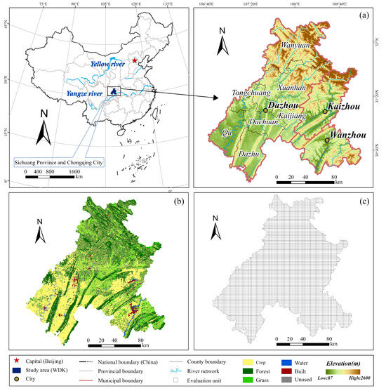
Figure 1.
Geographical location (a), land use status in 2020 (b), and 2 km evaluation unit map (c).
2.2. Data Sources and Processing
The Resource and Environment Science and Data Center of the Chinese Academy of Sciences provided the land use statistics used in this analysis for 1980, 1990, 2000, 2010, and 2020 (http://www.resdc.cn, accessed on 15 October 2024). The pixel size of these datasets is 30 m × 30 m, with an interpretation accuracy exceeding 90% [49]. The regional land use data were divided into six types using the ArcGIS 10.8 reclassification tool, which adheres to the primary classification standard: Crop, Forest, Grass, Water, Built, and Unused.
The Digital Elevation Model (DEM) data were sourced from the global 30 m resolution DEM dataset released by NASA in 2020 (https://lpdaac.usgs.gov/products/nasadem_hgtv001/, accessed on 25 October 2024) [50]. All datasets underwent coordinate system standardization using ArcGIS 10.8 software to ensure spatial consistency. In addition, the population and GDP data for the WDK region during the study period were sourced from the local government statistical departments of Dazhou and Chongqing [51,52].
2.3. Methodology
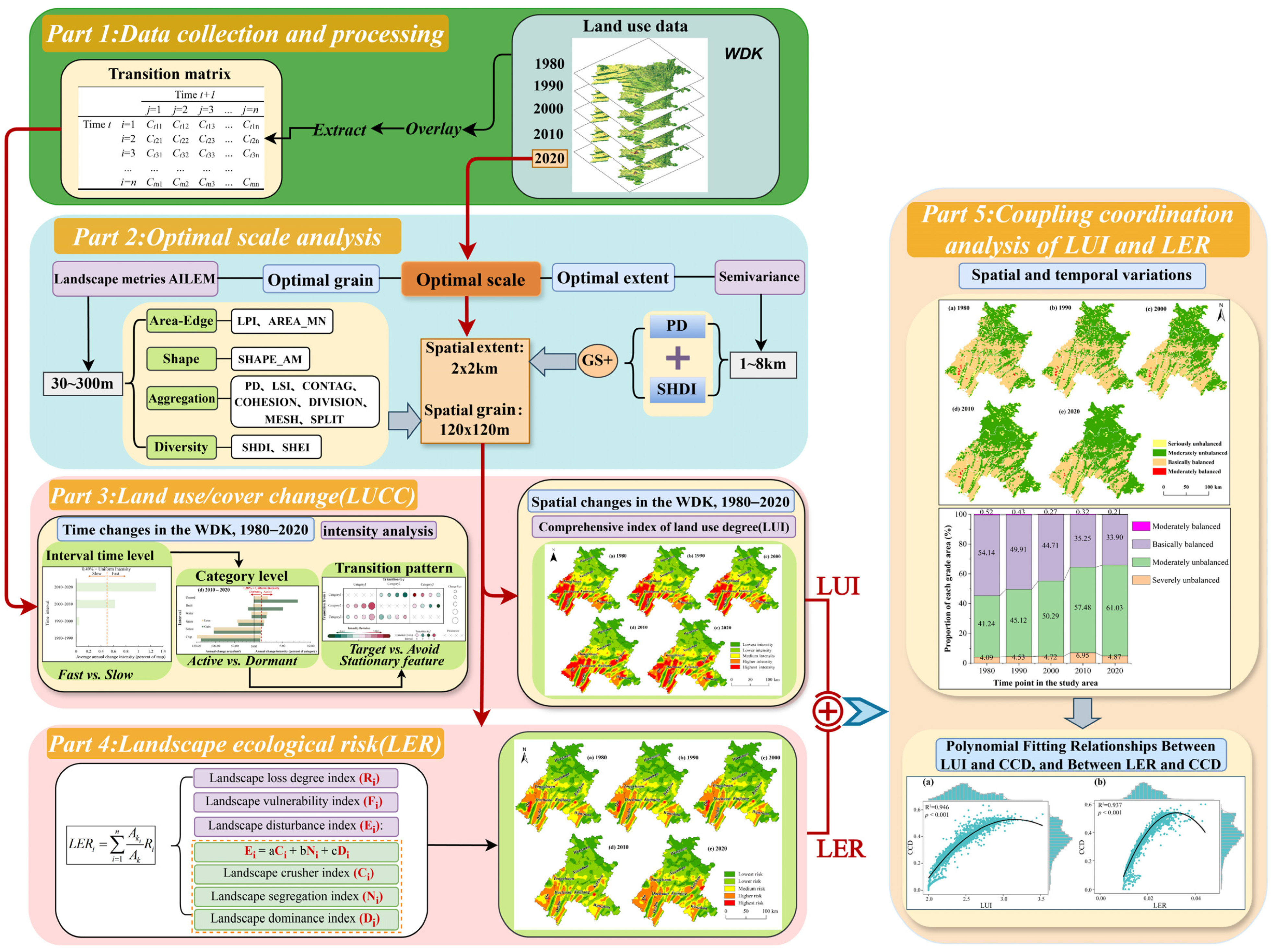
Figure 2 outlines our study process in five parts: (1) Creating a raster dataset from land use data and building a transition matrix. (2) Determining optimal spatial scale using 12 landscape metrics, the area information loss estimation model, and semivariogram analysis. (3) Conducting LUCC study, using intensity analysis for temporal features and land use index for the spatial distribution of LUI in WDK. (4) Evaluating ecological risk level in WDK using landscape metrics at the optimal scale. (5) LUI and LER’s coupling and coordination degrees were explored in spatial and temporal dimensions.
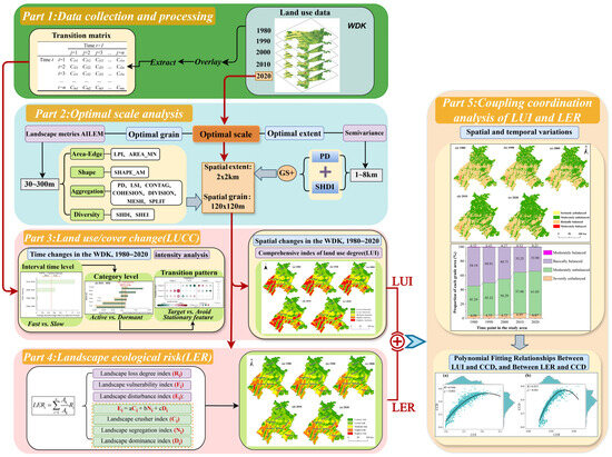
Figure 2.
Research framework.
2.3.1. Effects of Spatial Scale
- (1)
- Division of fundamental and evaluative units
From the 2020 land use data, we created several raster datasets using ArcGIS 10.8’s resampling feature. Ten different datasets were produced by methodically resampling the initial 30 m resolution data, with spatial resolutions gradually rising from 30 m to 300 m at 30 m intervals. Moreover, drawing on the research experience of previous scholars, it is advisable to delineate evaluation grid cells at 2–5 times the average patch size of the study area. To identify the most suitable assessment unit for the WDK region, we utilized ArcGIS 10.8’s Fishnet functionality. This tool facilitated the creation of a series of grids comprising eight different spatial extents. The grid sizes ranged from 1 km to 8 km, with incremental increases of 1 km between each successive extent [28,44].
- (2)
- Area Information Loss Estimation (AILE) Model
Drawing upon an extensive literature review and considering the unique features of our study region, we identified a set of 12 landscape metrics encompassing four key categories at the landscape scale: landscape diversity, area edge, shape, and spatial aggregation. These metrics were computed and examined using Fragstats version 4.3. We employed the AILE model to objectively ascertain the analysis’s most appropriate grain size [44,53].
where is the relative loss value of the landscape area of category . and are areas of category landscape before and after the change. is the information loss index of the landscape area in the study area, and n is the six landscape categories in the study area.
- (3)
- Semivariogram
The semivariogram function, a fundamental geostatistical tool, quantifies the spatial variance between data points as a function of distance [54]. In the research, we selected two landscape metrics: Patch Density (PD) and Shannon’s Diversity Index (SHDI) [28,44]. We utilized GS+ software (Version 9) to fit semivariogram functions for PD and SHDI at various grid scales to determine our analysis’s optimal spatial evaluation scale.
where denotes the calculated semivariogram value, represents the regionalized variable, is the set of all sample pairs at lag distance , and and are the variable values at locations and , respectively.
2.3.2. Intensity Analysis
There are three levels in the intensity analysis model. The intensity of land use change throughout each period may be assessed using the interval level. Whether each land use type’s gain or loss is in an active or dormant state of change is described at the category level. A more detailed representation of whether migrations from other categories to a particular category are trending or avoiding is given by the transition level [15,55].
(1) The average change intensity over the research period, and the land use change intensity for every time interval are quantified at the interval level. When > , it indicates that the change during that particular time interval is fast; when < , it suggests that the change is slow.
(2) The category level estimates the yearly gain intensity or loss intensity for every land use category across various period intervals. According to Equation (4), and are compared with to determine the activity state of each category. If > , the Category land use area gain is active; if > , the Category land use area loss is active. Conversely, if < or < , the gain or loss changes belong to a dormant state.
(3) The transition level builds upon the preceding two levels, further investigating the intensity of transitions from other categories to a specific category , as well as the uniform intensity of transitions to category . If > , it indicates that category aims to transition to category ; conversely, if < , it suggests that category avoids transitioning to category .
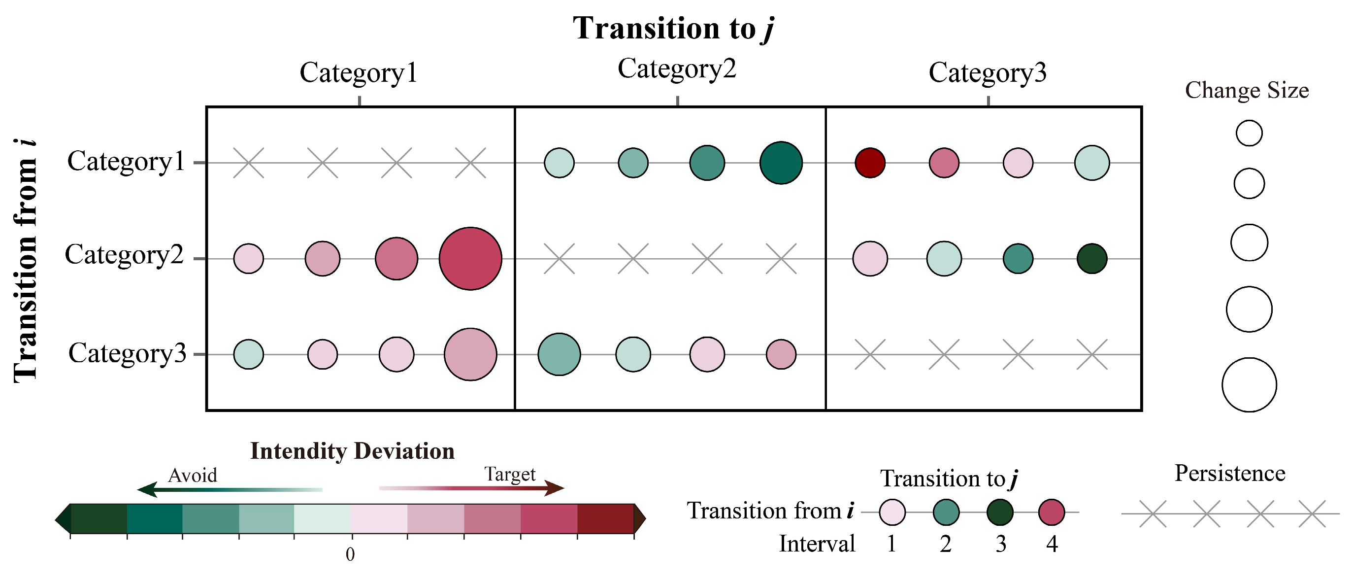
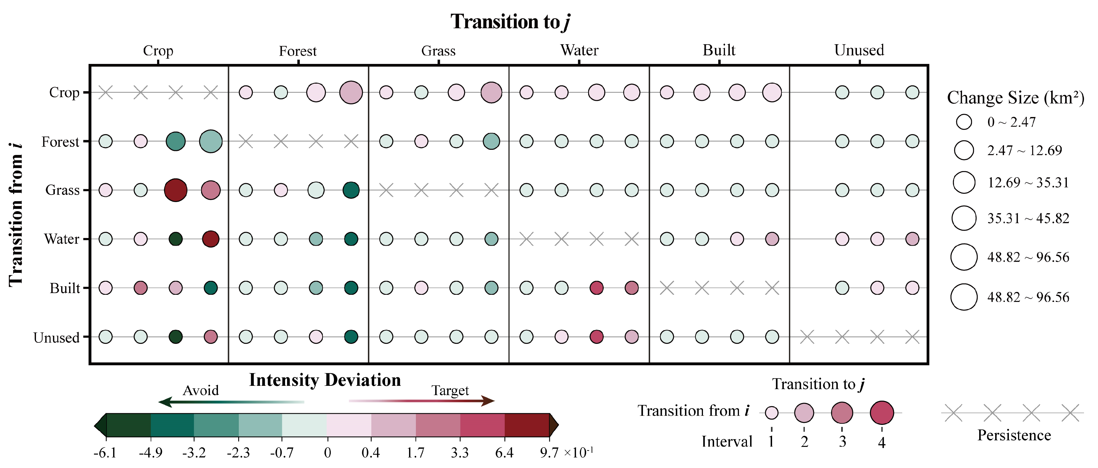
The transition pattern [19,21] visually represents inter-category transition disparities, facilitating the identification of transition characteristics. By calculating the difference between the transition intensity to category and the uniform transition intensity , we derive the deviation intensity , which indicates the avoidance or tendency of land use category transitions. This study used R software (version 4.4.2) to visualize each land use category’s transition areas and intensities across various time intervals. Transition areas and intensities were categorized into five categories using the natural break point technique. The bubble color indicates the transition’s tendency or avoidance status, whereas the magnitude of the bubble indicates the transition areas between land use categories (Figure 3). The vertical axis represents the starting time point of the study period, and the horizontal axis indicates the end time point.
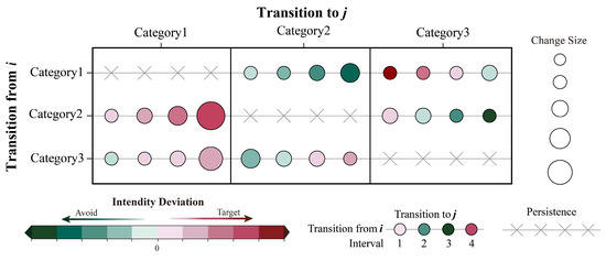
Figure 3.
Transition pattern.
In Equations (4)–(10), denotes the number of land use categories; stands for the whole study period; during the interval − , the area changing from land use category to category is denoted by ; stands for the area changing from category to a specific category during − ; shows the area transitioning from any category to category during − ; , , and represent the unchanged areas of categories , , and , respectively, during − .
2.3.3. Comprehensive Index of LUI
This study divided land use types into four classes and assigned corresponding values based on prior research experiences and the specific characteristics of WDK: Crop 3, Water, Grass, and Forest (2 each), Unused 1, and Built 4 [22]. This categorization reflects the different levels of ecological effect and human intervention associated with the land use category.
In Equation (11), represents the index of LUI, denotes the assigned value for every land use type; the percentage of every land use category to the total area is denoted by .
2.3.4. LER Assessment
When disturbed, different types of landscapes have varying increases in ecological risk, which the landscape loss index explains. We created an ecological risk assessment model based on this index to examine the spatiotemporal variability of ecological hazards in the WDK region (Table 1) [56,57].
2.3.5. CCD Model
Our research used the approach to assess how LUI and LER interact [58,59]. We standardized the data for each system to eliminate the dimensional differences between these two subsystems.
where represents the original value of a given subsystem, and denote the maximum and minimum original values within that subsystem index, and is the normalized result for that subsystem. represents the coupling degree, is the normalized value of the LER, and is the normalized value of the LUI. denotes the coordination degree, where and are the weights assigned to LER and LUI. Based on a review of numerous studies and considering the actual situation in the study area, LER and LUI are equally crucial for promoting regional sustainable development. Therefore, we set and to 0.5, respectively. represents the value of CCD. We classified the CCD, as shown in Table 2 [39,55,56].

Table 1.
The formula for LER calculation.
Table 2.
CCD types between LUI and LER.
3. Results
3.1. Spatial Effect Analysis
3.1.1. Spatial Grain Analysis
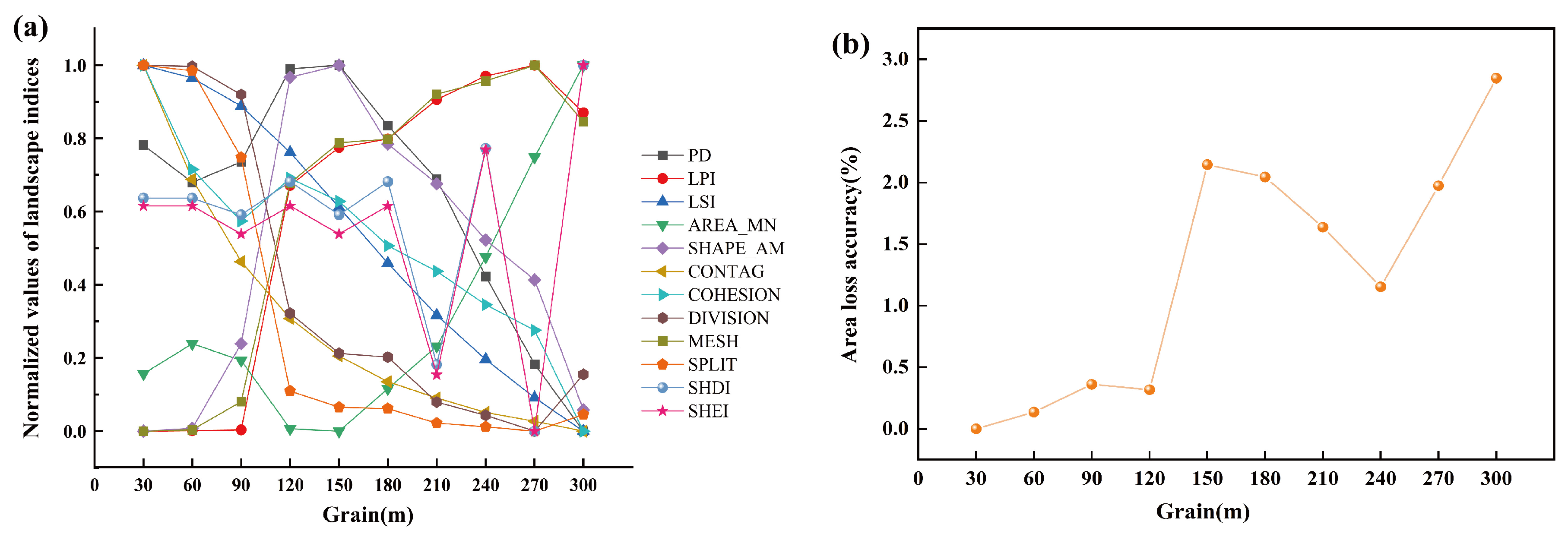
Figure 4a illustrates the normalized results of twelve landscape metrics. The indices exhibited differentiated response characteristics: LSI, CONTAG, and COHESION steadily decreased over the 30–300 m grain range, devoid of notable variations. LPI and MESH showed minimal fluctuations within the 30–90 m range but rapidly increased and stabilized between 90 and 120 m. SPLIT and DIVISION values decreased rapidly and monotonically within the 30–120 m range, then stabilized after an inflection point at 120 m. SHEI and SHDI exhibited similar fluctuation trends, with minimal variations in the 30–180 m grain range and dramatic fluctuations beyond 180 m, indicating significant size influence. SHAPE_AM, PD, and AREA_MN reached their respective maxima and minima within the 120–150 m range. Based on these response curve characteristics, we preliminarily determined the suitable spatial grain interval to be 120–150 m.
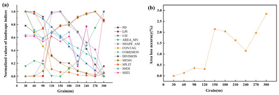
Figure 4.
Response curves of different landscape metrics (a) and landscape area loss index (b) under spatial resolutions from 30 to 300 m.
Figure 4b shows that at spatial resolutions exceeding 120 m, the landscape area loss index exhibits substantial fluctuations, consistently surpassing the 1% threshold. As the spatial grain decreased, WDK’s landscape composition stability improved. Within the 30–120 m grain range, the landscape area loss index showed only slight fluctuations, with calculated values below 0.5%. Specifically, the index increased monotonically from 30 to 90 m, then decreased between 90 and 120 m, with the area loss index at 120 m smaller than 90 m. Considering these analyses comprehensively, we determined the optimal spatial grain for the study area to be 120 m.
3.1.2. Spatial Extent Analysis
Through comparative analysis of multiple model fitting effects, this study determined that the Gaussian model performed optimally in capturing spatial autocorrelation information. Table 3 presents the calculation results for PD under the Gaussian model fitting. Across spatial extents from 1 to 8 km, the Nugget Variance (Co) decreased from 2.569 to 0.136, while the Structural Variance sill (Co + C) reduced from 9.400 to 1.899. This phenomenon suggests that smaller spatial partitions may disrupt the initial form of the study area, potentially leading to the loss of crucial information. The Co/(Co + C) ratio initially increased in the 1–2 km extent, followed by a brief decline in the 2–3 km extent. Subsequently, within the 3–8 km extent, the Co/(Co + C) ratio increased from 0.778 to 0.928. A higher Co/(Co + C) ratio indicates more significant spatial heterogeneity caused by random variables in landscape structural elements. Concurrently, the R2 fitting value at the 2 km spatial extent was 0.995, surpassing the R2 fitting value of 0.955 at the 3 km extent, thus achieving optimal fitting performance. Considering that RSS values remained relatively small across all fitting scales, the 2 km spatial evaluation extent more accurately reflects the spatial variability of the PD.
Table 3.
Semivariogram information of the PD at different spatial extents.
Table 4 illustrates the calculation results for SHDI under the Gaussian model fitting. Within the 1–2 km spatial extent, Co decreased from 0.074 to 0.061 as the extent increased. Co started to climb progressively as the geographical extent rose from 2 to 8 km, suggesting increased spatial heterogeneity caused by randomness. The lowest Co/(Co + C) values across all spatial extents were observed within the 1–3 km spatial extent; given that the R2 value reached its maximum of 0.961 at the 2 km spatial extent, with RSS maintaining a relatively low value, the 2 km spatial extent effectively reflects SHDI spatial diversity. Notably, some spatial information may be lost at wider geographical extents. According to the above results and analysis, 2 km was selected as the optimal extent for the research area.
Table 4.
Semivariogram information of SHDI at different spatial extents.
3.2. Examination of Land Use Transformations
3.2.1. Analysis of Land Use Changes over Time
- (1)
- Dynamics of Land Use Composition and Interval Levels
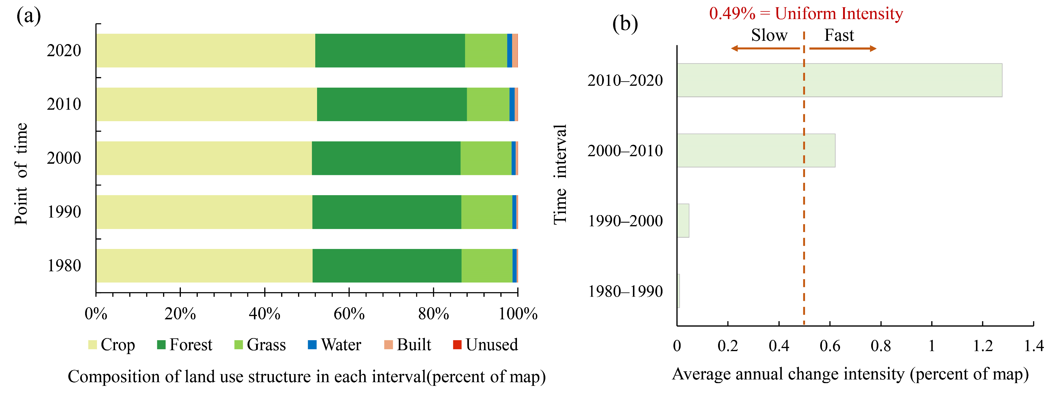
Figure 5 illustrates the structural and intensity changes in land use in WDK from 1980 to 2000. As depicted in Figure 5a, Crop was the most common land use type, covering 51% of the total area during the research period (1980–2020). Thus, agriculture has maintained its dominance in the area. Forest and Grass collectively showed a 1.89 percentage point reduction in area coverage. Built showed a significant expansion, increasing from 0.26% to 1.29%, reflecting increased urbanization.
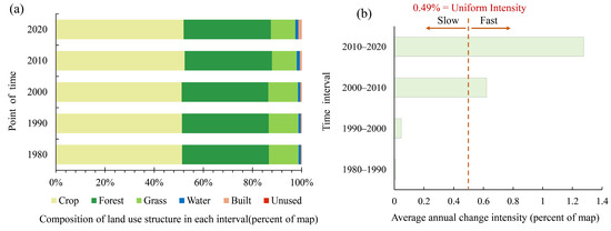
Figure 5.
Land use structure (a) and level of change intensity of time intervals (b) in WDK from 1980 to 2020.
Figure 5b depicts the WDK region’s land use change intensity from 1980 to 2020, illustrated in Figure 5b, with the red dashed line representing the mean yearly change intensity of 0.49%. The period from 1980 to 2000 exhibited change intensities below the mean annual rate, indicating a state of slow transition. In contrast, the subsequent two decades (2000–2020) witnessed change intensities surpassing the mean yearly rate, signifying a rapid phase of land use transitions. These characteristics suggest that anthropogenic activities induced relatively minor land use changes during the initial 20-year period, followed by a gradual intensification in the latter 20 years.
- (2)
- Changes in Category Levels
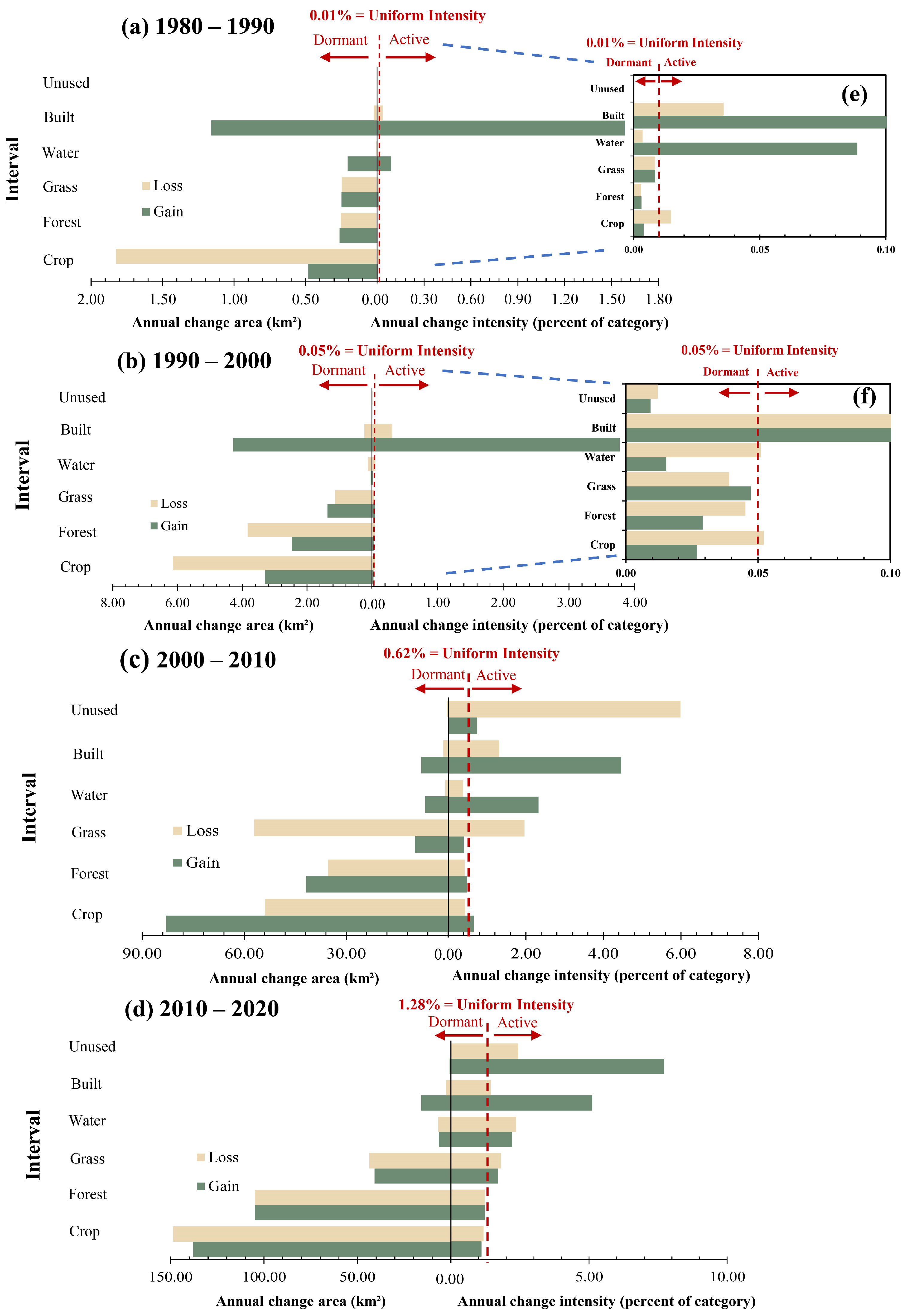
Figure 6 shows the area change and intensity of each land use type in the WDK region over the past 40 years. The yearly intensity of land use change was minimal between 1980 and 1990, at only 0.01%. Figure 6a shows that Built and Water generally increased while Crop decreased. Forest and Grass maintained a balanced change, and Unused showed insignificant variations. Built’s increase and decrease intensities were active, as were the increase in Water and decrease in Crop. Other land use categories exhibited dormant change intensities. Figure 6b reveals a notable decrease in Forest from 1990 to 2000. As shown on the right side of Figure 6b and the change intensities in Figure 6f, the reduction in the water area was slight. However, it exceeded the red dashed line, indicating an active change state. As depicted in Figure 6c, 2000–2010 witnessed a continuous expansion of Built, a significant loss of Grass, and overall increases in Water, Crop, and Forest. The change intensities of Unused, Built, Water, Grass, and Forest all surpassed the red line, indicating a substantial escalation in human activity intensity compared to the previous time interval. Figure 6d shows further increases in Built with active intensity. At the same time, Crop, Forest, Grass, and Water maintained overall balance in area changes, albeit with magnitudes far exceeding previous periods.
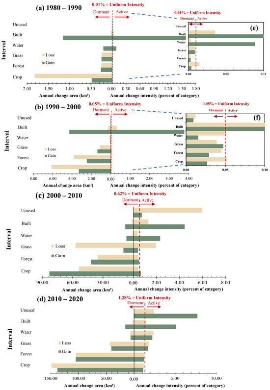
Figure 6.
Annual average change intensity of WDK land use category from 1980 to 2020 (a–d), category levels intensity magnification for 1980–1990 (e) and 1990–2000 (f).
Over the 40 years from 1980 to 2020, the degree of land use change intensified continuously, with the average change intensity rising from 0.01% to 1.28%. Built consistently expanded with increasing change intensity, while ecological land uses such as Crop, Forest, Grass, and Water maintained active change states in most intervals.
- (3)
- Changes in Transition Levels
The transition patterns during the research are depicted in Figure 7. From 1980 to 2020, Crop areas generally exhibited a target transition towards Forest, Grass, Water, and Built while avoiding transitions to Unused. For most of the research period, Forest consistently avoided transitioning to other land use categories, with a steadily increasing avoidance of transitioning to Crop and Grass. Similarly, Grass predominantly targeted transitions to Crop. This tendency was particularly pronounced from 2000 to 2010 when the target propensity and area of Grass-to-Crop transitions were high. From 1980 to 2020, Grass consistently avoided transitions to other land use categories. Water consistently avoided transitions to Forest and Grass throughout the study while targeting transitions to Unused. After 2010, Water began targeting transitions to both Crop and Unused.
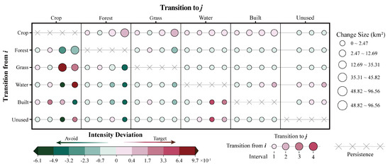
Figure 7.
Land use transition pattern of WDK from 1980 to 2020.
In summary, Crop served as the primary source for ecological land uses while avoiding transitions to Unused. The target intensity of Unused transitioning to Water gradually increased, which may positively affect the regional environment. However, the expansion of Built largely occurred through the encroachment on Crop and Water, potentially leading to land fragmentation and posing potential ecological risks.
3.2.2. Spatial Analysis of Land Use Changes
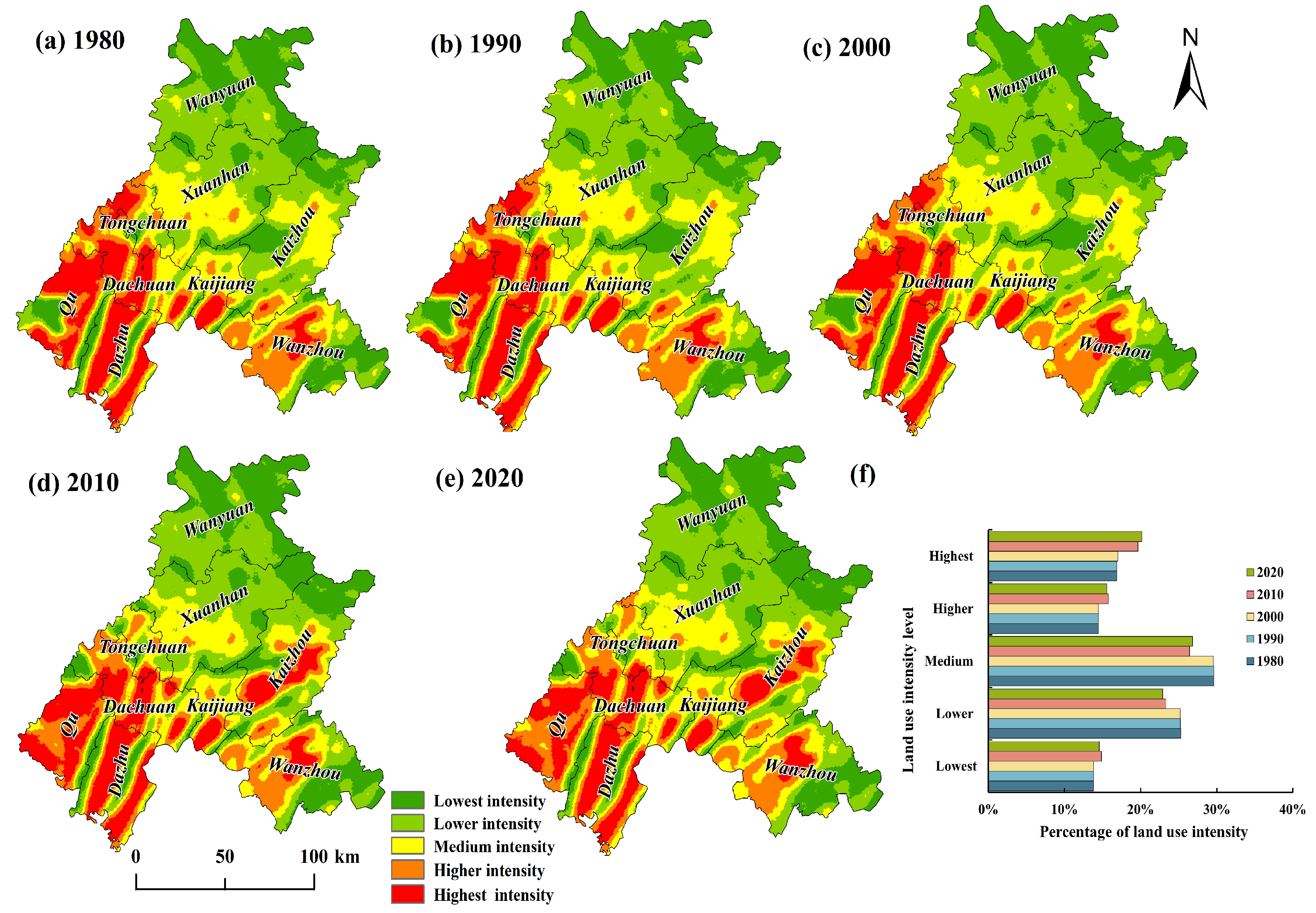
The research area was divided into 6386 evaluation units using a 2 km grid. The LUI in the WDK region was evaluated by calculating the land use degree index for every assessment unit. The results were divided into five levels using the natural breaks approach: lowest intensity (182.59–222.22), lower intensity (222.22–241.24), medium intensity (241.24–260.66), higher intensity (260.66–284.43), and highest intensity (284.43–400.00). As illustrated in Figure 8 and Figure 9, we employed ordinary kriging interpolation, implemented through ArcGIS 10.8, to generate visual representations of the results.
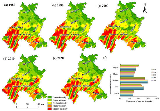
Figure 8.
Spatial distribution of land use intensity in WDK from 1980 to 2020 (a–e), percentage of land use intensity levels from 1980 to 2020 (f).
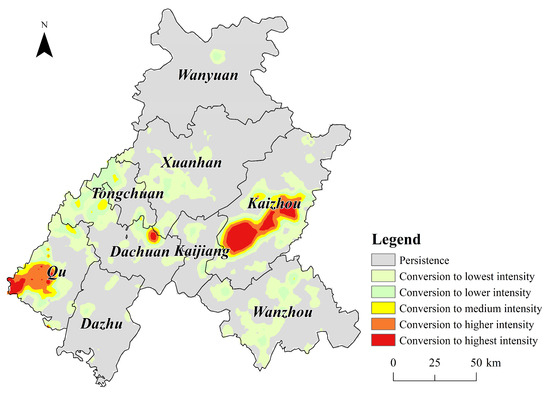
Figure 9.
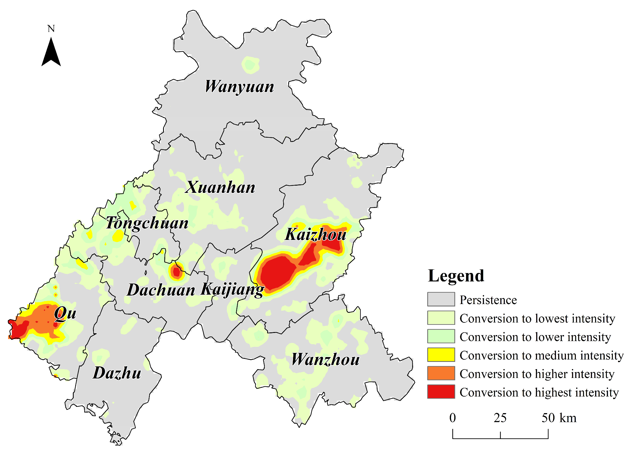
Spatial change map of land use intensity in WDK from 1980 to 2020.
The results indicate that medium- and low-intensity land use dominates the WDK region, including 38.5% of the overall study area, primarily distributed across the northern mountainous regions and the parallel mountain ranges in the central and southern parts. Higher and highest-intensity land use also occupies a significant proportion, approximately 33% of the WDK region, mainly concentrated in the parallel ridge–valley systems and hilly terrains of the central and southern regions, with an observed expansion towards the southwestern and eastern mountainous areas. As depicted in Figure 9, the period from 1980 to 2020 witnessed the emergence of new high-intensity land use zones, primarily concentrated in the urban construction areas of Qu and Kaizhou. This spatial pattern underscores the substantial impact of urbanization and agricultural development on land use intensity. New medium- and low-intensity areas were identified in Wanyuan, Dachuan, western Tongchuan, and eastern Wanzhou, indicating a relative decrease in the intensity of human-induced land surface modifications in these regions, which is conducive to improving environmental quality.
3.3. Spatiotemporal Changes in LER
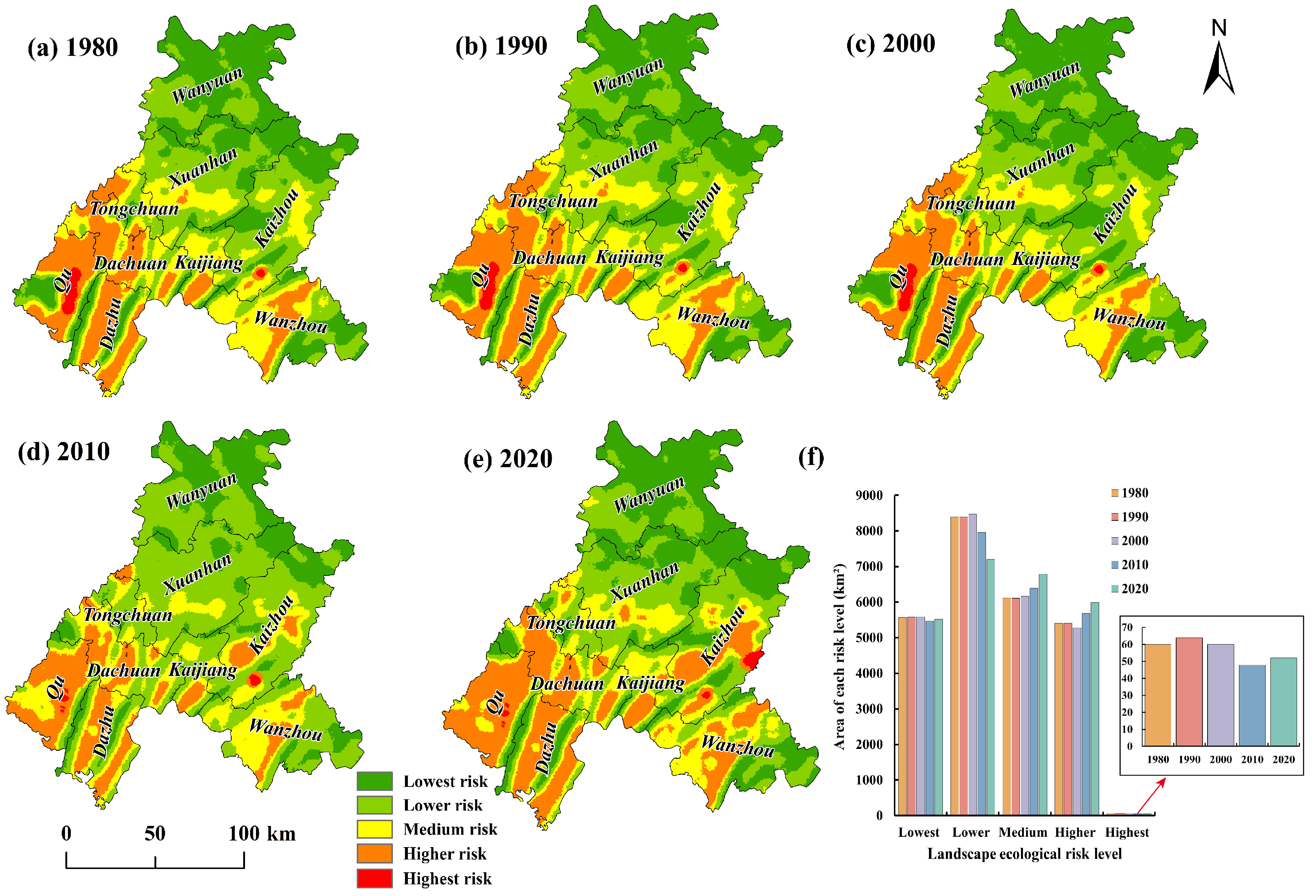
Figure 10 shows the spatiotemporal structure of LER in the WDK area based on a 2 km grid. Using the natural breaks approach, the LER was divided into five classifications: lowest (0.010–0.015), lower (0.015–0.019), medium (0.019–0.024), higher (0.024–0.056), and highest (0.056–0.185). The results indicate that while medium- and low-risk areas predominate in the WDK region, the proportion of high-risk areas increases. Low-risk areas cover 12,626.40 km2 (51.22%), medium-risk areas 6220.20 km2 (25.23%), and high-risk areas 5806.60 km2 (23.55%).

Figure 10.
Spatiotemporal distribution of LER in WDK from 1980 to 2020 (a–e), area of different LER levels from 1980 to 2020 (f).
Temporal analysis reveals that low-risk areas remained stable from 1980 to 2000 but decreased thereafter, with a significant reduction observed between 2010 and 2020, gradually transitioning into high-risk areas. As shown in Figure 11, newly emerged high-risk areas are primarily found in densely populated urban zones, such as central Kaizhou and southwestern Qu. Conversely, new low-risk areas are mainly distributed in Wanyuan, southwestern Dachuan, and western Tongchuan. This ecological risk distribution pattern aligns with the spatial changes in LUI, suggesting a correlation between the two factors.
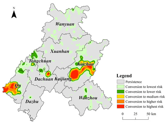
Figure 11.
Spatial change map of LER in WDK from 1980 to 2020.
Spatially, low-risk areas are mainly located in the parallel mountain ranges of northern, eastern, and southwestern WDK, characterized by Forest and Grass with favorable ecological conditions. Most medium-risk areas are in the middle of Crop and periphery of Built, where land use type conversions have induced moderate environmental risks. Urban built-up zones and places with high human activity, including Crop and Grass, are the central locations for high-risk areas. The high intensity of land use transition has caused landscape fragmentation in these areas, resulting in elevated ecological risks.
3.4. CCD Analysis of LUI and LER
A unified 2 km evaluation scale was used to compute the CCD between LUI and LER. The CCD between LUI and LER in the WDK region ranged from 0 to 0.8, and was primarily categorized into four types: seriously unbalanced (0–0.2), moderately unbalanced (0.2–0.4), basically balanced (0.4–0.6), and moderately balanced (0.6–0.8). Figure 12f demonstrates that moderately unbalanced and basically balanced states predominantly characterized the WDK region throughout the study period. Between 1980 and 2020, the percentage of moderately unbalanced areas grew steadily from 41.24% to 61.03%. Concurrently, the overall proportion of basically balanced regions decreased from 54.14% to 33.90% over the entire study period from 1980 to 2020. Figure 12a–c, f reveal that the proportion of basically balanced areas was approximately 50% from 1980 to 2000, but moderately unbalanced areas progressively replaced this during the 2000–2020 period (Figure 12d–e).
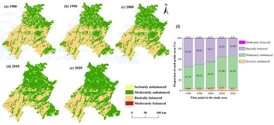
Figure 12.
Distribution and area proportion of WDK coupling coordination degree from 1980 to 2020 (a–e), percentage of coupling coordination degree levels from 1980 to 2020 (f).
Table 5 presents the average CCD levels for each year, indicating a generally low coupling and coordination level over the 40 years. Although the coupling correlation between land use changes and ecological risk formation was high across all periods, the degree of coordinated development remained low. The observed patterns reveal a significant interrelationship between LUI and LER systems. Mitigating ecological vulnerabilities hinges on fostering coordination between these two interlinked systems. Furthermore, the ratios of seriously unbalanced and balanced development stayed mostly constant, suggesting that the environmental hazards brought on by changes in land use may have been primarily confined to specific areas throughout the study period.
Table 5.
The average level of CCD between LUI and LER.
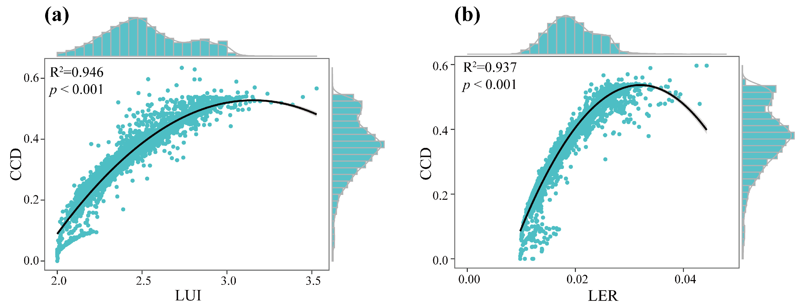
Between 1980 and 2020, the spatial distribution of the coupling coordination degree (CCD) between LUI and LER in the WDK region exhibited an overall pattern characterized by lower values in the north and higher values in the south. The central, southeastern, and southwestern areas of the WDK region, as shown in Figure 13, correspond to high values of both LUI and LER. Intensive human activities and a high proportion of Built and Crop characterize these areas. To demonstrate the specific relationship between CCD and LUI, as well as between CCD and LER, we used R software (version 4.4.2) to plot the fitting curves of CCD with LUI and LER (Figure 13) [64]. The polynomial-fitted R2 values were all greater than 0.93, and the p-value was less than 0.001, indicating that the fitting curves have high explanatory power in describing the CCD process in relation to both LUI and LER. Most values of LUI and LER are distributed to the left of the fitted quadratic function, where an increase in LUI and LER is associated with an increase in CCD. There is a significant positive correlation between CCD and both LUI and LER. An increase in LUCC intensity leads to the expansion of severely unbalanced and moderately unbalanced areas. At the same time, a decrease in LER reduces seriously unbalanced, moderately unbalanced, and basically balanced areas. A small portion of the data from the basically balanced area are distributed to the right of the inflection point of the fitting function. This phenomenon suggests that, beyond the inflection point, further increases in LUI and LER result in a weakening of their coupling and coordination. However, the distribution density of the data indicates that these values do not alter the overall positive correlation between CCD and both LUI and LER. Therefore, it is crucial to closely monitor land use practices in areas currently at a moderately balanced or balanced development stage, avoiding excessive encroachment on ecological lands such as Forest and Grass to prevent further ecological degradation.
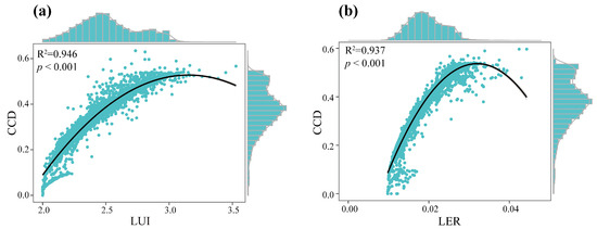
Figure 13.
The fitting curves and distribution density of CCD with LUI (a) and LER (b).
4. Discussion
4.1. LUCC Process at Spatiotemporal Scales
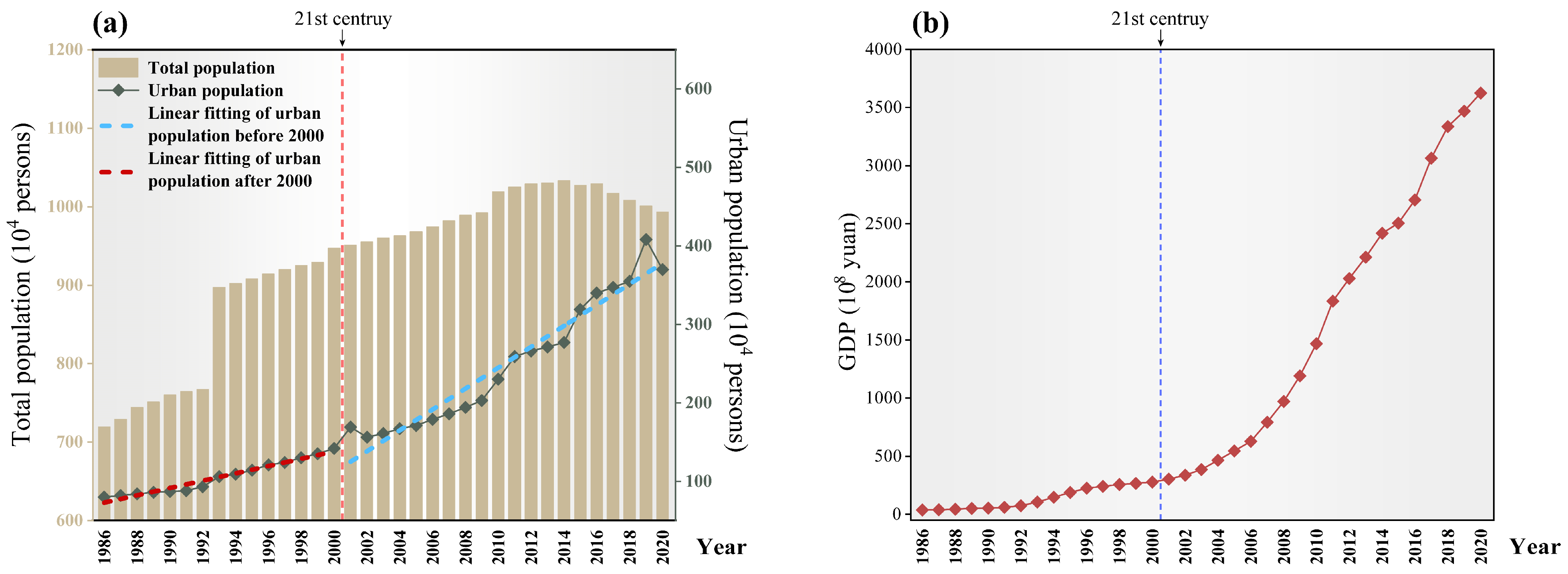
Figure 5, Figure 6 and Figure 7 illustrate that the LUCC in WDK underwent complex evolution over the past 40 years. The LUCC process can be divided into two distinct phases, with the year 2000 as a pivotal point. Between 1980 and 2000, the LUCC intensity was relatively low and changed slowly. The LUCC intensity increased rapidly, with the annual rate of change from 2010 to 2020 reaching its peak (Figure 5b). These LUCC dynamics are likely closely associated with population growth and economic development. At the transition level (Figure 7), the trend of Crop transitioning to Built remains stable. Although Forest, Grass, and Water contributed to the growth of Built, Crop remained the primary stable source rather than other land use types. Two possible reasons account for this: firstly, WDK, as a typical grain-producing area, had a sizeable initial cropland area; secondly, influenced by topography, WDK’s urban areas were primarily located near grain-producing regions, with forestland and grassland distributed in hilly areas surrounding cities. Urban expansion mainly occurred towards flat cropland areas, with minor expansion into hilly regions. As shown in Figure 14a, WDK’s population has steadily increased since 1986, with the total population growing from approximately 7.2 million to 10 million. The fitted curve for urban population growth in the region indicates that the urban population growth rate during 2001–2020 was approximately triple that of 1986–2000, with the urban population expanding from 800,000 to 3.7 million. As the 21st century began, WDK entered a rapid economic development phase characterized by exponential growth (Figure 14b) [51,52]. The accelerated GDP growth and urbanization process have been mutually reinforcing, leading to substantial rural-to-urban migration and increasing housing, transportation, and infrastructure demand. This surge can be attributed to the deepening implementation of “Western Development” strategies and the industrial transformation brought about by the Three Gorges Project. The development of industrial and agricultural economies has driven the rapid expansion of urban areas and transportation infrastructure to accommodate human activities [65,66].
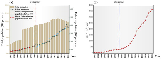
Figure 14.
Population changes (a) and GDP growth trends (b) in WDK.
In addition, when research involves multiple periods and land use types, traditional conversion hierarchy visualization methods require generating numerous bar charts [15]. This situation makes it challenging to identify LUCC characteristics systematically. This study overcame the limitations of traditional conversion hierarchy visualization methods by introducing the “transition pattern” concept and utilizing R language technology [19]. This approach clearly expresses the overall trend of land use type conversions, thereby better explaining the growth process of Built.
Based on the comprehensive index of land use degree, the LUI calculation effectively elucidates the spatial influence of human activities on various land types. This approach may address the limitations of conventional intensity analysis, which often falls short in spatial analysis. The integration of intensity analysis and the comprehensive land use intensity index offers two distinct advantages: Spatially, the comprehensive land use intensity index reveals the distribution of areas with intensive human activity. These regions typically feature more prominent and concentrated Built and Crop, indicating higher land use intensity. Temporally, intensity analysis elucidates the magnitude of land use type transitions driven by human activities within these areas.
4.2. Comparative Analysis of LER Characteristics
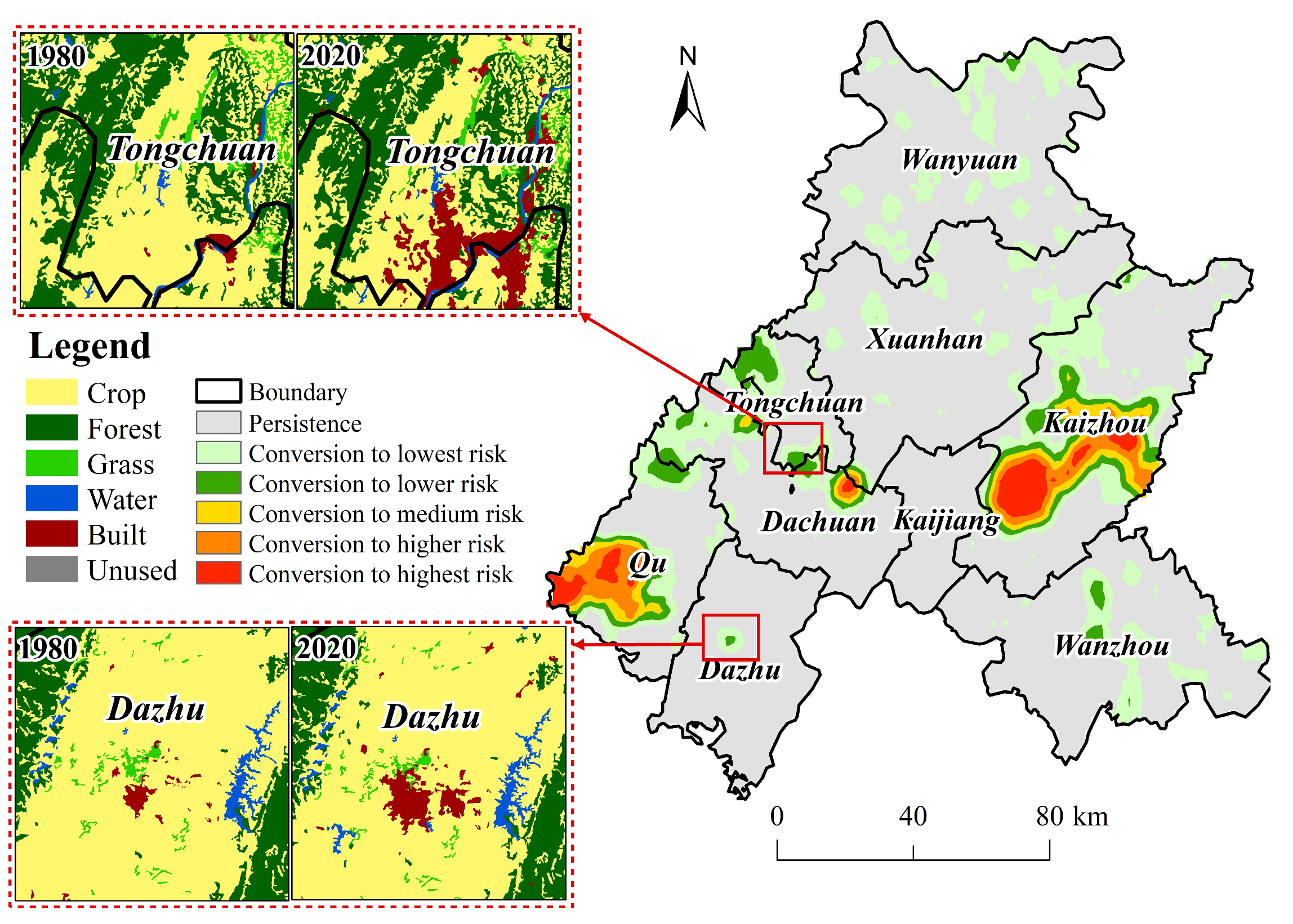
Conducting LER assessment at the optimal evaluation scale enables the detection of subtle changes and spatial heterogeneity within the study area. The research indicates that over time, the risk gradient evolution in the central urban areas of Dazhu and Tongchuan exhibits patterns contrary to classical theoretical expectations. High-risk patches in these areas show a gradual transition towards medium and low-risk characteristics (Figure 10), with this trend being particularly pronounced in Dazhu’s central urban area. However, some studies have found densely populated urban areas are not necessarily associated with the highest landscape ecological risk values [37,67].
Considering the actual situations depicted in Figure 1 and Figure 15, the central urban areas of Dazhu and Tongchuan are characterized by flat terrain with no major rivers or mountains fragmenting the Built, facilitating Built’s concentrated and contiguous expansion. Additionally, the land use types surrounding these central urban areas are relatively homogeneous, resulting in landscape fragmentation affecting fewer land categories as construction land expands. Although the landscape is predominantly artificial and exerts considerable disturbance on the ecological environment, after 40 years of rapid urbanization, the distribution of Built in these central areas has become concentrated and less susceptible to changes induced by human activities or natural environmental factors. Consequently, the ecological risk values are relatively low.
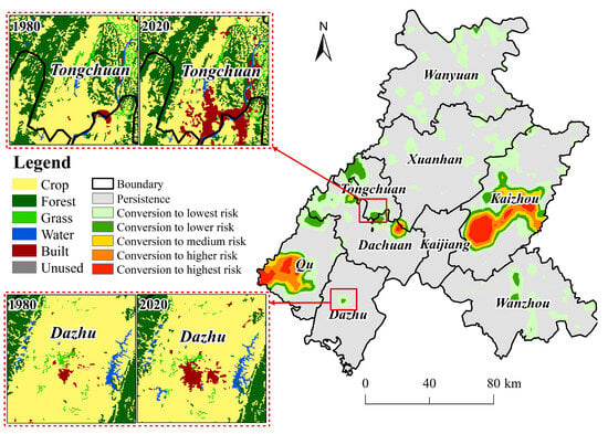
Figure 15.
Land use changes with significant ecological risk anomalies in 1980 and 2020.
Interestingly, the ecological risk in the nearby farmland and grassland is still rising, even while the growth of central metropolitan districts in both regions has leveled off. These phenomena indicate that the pattern of construction land expansion has shifted from a single-center outward growth to a multi-nodal network sprawl, signifying a new stage in the evolution of regional human–land relationships.
4.3. Interaction Between LUI and LER
The results reveal significant spatial heterogeneity in the coupling relationship between LUI and LER in the WDK region. Spatially, the CCD values exhibit a “low in the north, high in the south” pattern, aligning with previous research [41,42]. However, our study employed a finer evaluation scale to analyze subtle CCD changes in the WDK region. Newly identified areas with low CCD values are primarily distributed in northern Wanyuan, Dachuan, Xuanhan, and western Tongchuan (Figure 12), highly overlapping with areas of low LUI-LER. This corroborates the effectiveness of Chinese government policies such as the Grain for Green Program and riparian zone restoration. LUI and LER have been reduced to relatively low levels in these areas. These measures contribute to protecting biological habitats and enhancing ecological security [68].
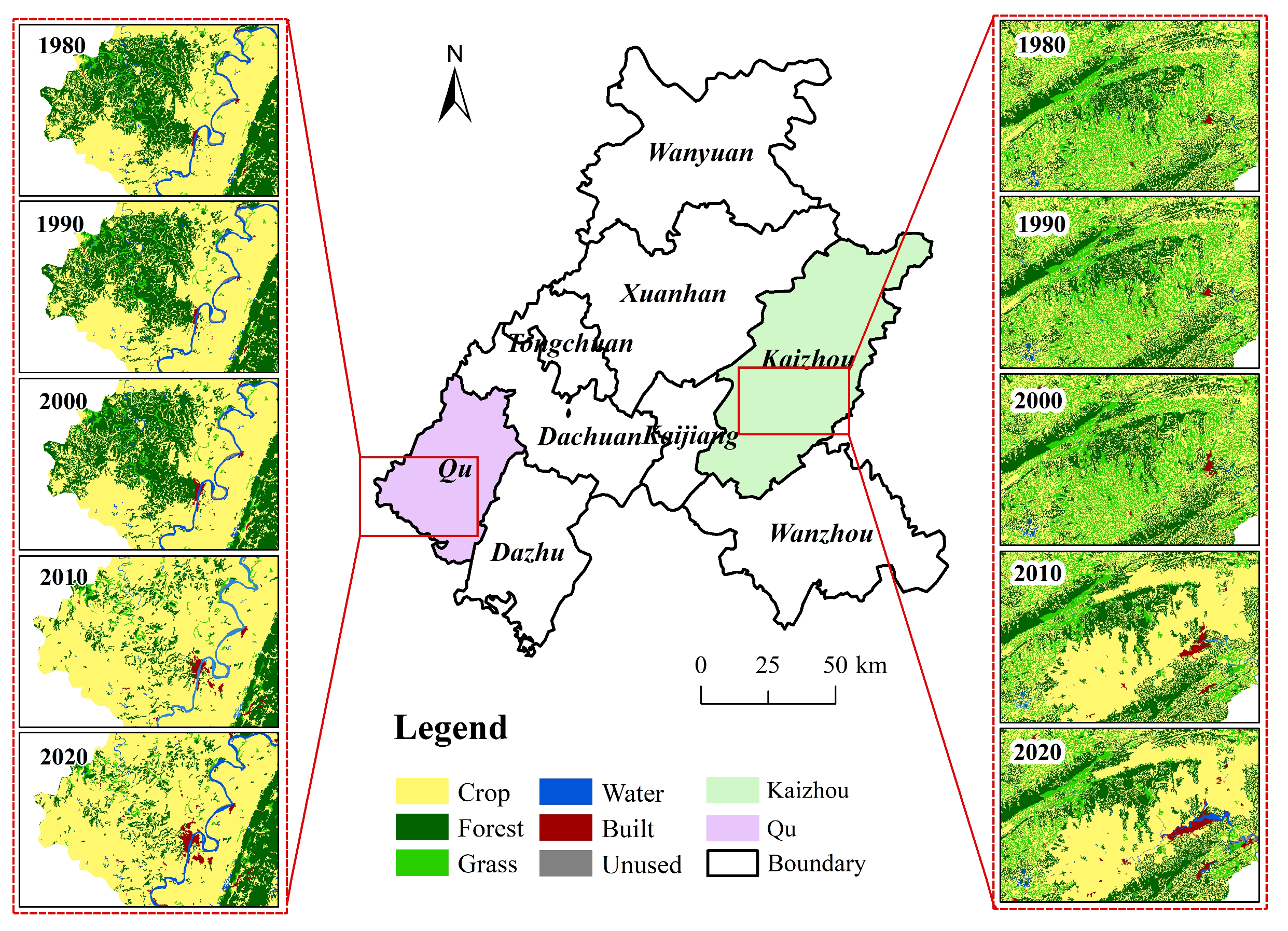
Despite the improved environmental quality in some areas, the coordination between LUI and LER has consistently remained low. This phenomenon indicates that the degradation of the ecological environment persists. We observed the appearance of concentrated red areas in Figure 9 and Figure 11, identifying two typical ecological deterioration zones in southwestern Qu and central Kaizhou. Over the past 40 years, CCD values in these areas have consistently increased, with values in central urban areas and surroundings remaining within the 0.4–0.8 range. We analyzed land use changes in Qu and Kaizhou over 40 years (Figure 16) and identified the following possible causes:
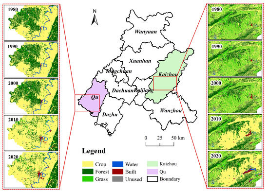
Figure 16.
Land use changes in areas with significant ecological deterioration from 1980 to 2020.
- (1)
- After 2000, rapid agricultural development in Qu County converted southwestern hilly areas into cropland. In Kaizhou, cropland development in the middle reaches of the Nanjiang River resulted in a significant reduction in forestland and grassland. These phenomena cause topsoil loss and may affect regional biodiversity and ecosystem integrity through food chain disruptions [69].
- (2)
- The central urban areas of both regions are distributed along the tributaries of the Yangtze and Jialing Rivers. Due to topographical constraints, urban expansion primarily occurred in flat areas near the riverbanks. Over the past two decades, rapid urbanization has reshaped the ecological processes of river corridors, and the expansion of artificial surfaces has fragmented existing ecological networks. These severe landscape disturbances have led to the fragmentation of many forest and grassland patches [70].
The comprehensive management of these ecological degradation zones is of typical significance for achieving high-quality development and meeting the UN Sustainable Development Goals (such as SDG 15.1 and SDG 15.3). Specifically, agricultural development on slopes exceeding 15 degrees should be restricted in the hilly areas of southwestern Qu. Economic tree species should be introduced to balance soil and water conservation with farmers’ livelihoods. For the fragmented ecological corridors along the river in central Kaizhou, it is recommended to maintain continuous vegetation buffer zones of at least 50 m wide on both sides of the tributaries. Additionally, artificial wetlands should be integrated to connect fragmented habitats [71,72].
4.4. Limitation
Our research provides helpful information on land management and ecological governance in the study area. However, this research has certain limitations. Our research mainly examined the effects of LUCC on LER without fully considering other potential factors, such as transportation network layout, soil type distribution, and climate change trends in the study area. Therefore, we suggest constructing a comprehensive indicator system tailored to the WDK region. Building upon this foundation, we intend to simulate risk distributions under multiple future scenarios and develop a rational ecological security pattern that harmonizes ecological protection with socioeconomic development.
5. Conclusions
- (1)
- Over the 40 years, the main land use types in the WDK region were Crop and Forest. The increase in Built within the WDK region was consistently active, with the change intensity expanding 128-fold. Crop was the primary stable source for this expansion. Evident trends of mutual conversion were observed among Crop, Grass, and Water, with Crop serving as the primary source for increases in Forest, Grass, and Water. Notably, Crop remained stable, avoiding conversion to Unused.
- (2)
- LUI and LER spatial distributions exhibited a consistent south-high, north-low pattern. Medium- and low-intensity areas predominantly occupied high-altitude mountainous regions, while high-intensity areas concentrated in Crop and Built. Emerging high-risk areas were mainly distributed in Qu’s urban construction area, western hills, and central Kaizhou. Concurrently, Dazhu and Tongchuan’s central urban expansion stabilized, accompanied by reduced ecological risk. Built-up area expansion evolved from single-center outward growth to multi-nodal network expansion. The optimal landscape pattern for WDK was determined at a 120 m grain size and 2 km extent.
- (3)
- The CCD between LUI and LER predominantly manifested as moderately unbalanced and basically balanced types, characterized by strong coupling–weak coordination states. The proportion of moderately unbalanced areas increased, while that of basically balanced areas decreased. Although some regions experienced improvements in their ecological environment, there was a notable deterioration in the central area of Kaizhou, as well as in the urban sections of Qu and its hilly western portions.
Author Contributions
Conceptualization, B.Q. and D.Z.; methodology, D.Z.; software, D.Z. and J.L.; validation, D.Z., B.Q. and J.L.; formal analysis, D.Z.; investigation, D.Z. and J.L.; resources, B.Q.; data curation, D.Z.; writing—original draft preparation, D.Z.; writing—review and editing, B.Q., D.Z. and J.L.; visualization, D.Z. and J.L.; supervision, B.Q.; project administration, B.Q.; funding acquisition, B.Q. All authors have read and agreed to the published version of the manuscript.
Funding
This research was funded by the Key Project of the Social Science Foundation of Hengyang under grant number 2021B(I)004 and the Major Project of the Key Project of Hunan Provincial Department of Education (17A067).
Institutional Review Board Statement
Not applicable.
Informed Consent Statement
Not applicable.
Data Availability Statement
The data used in this study can be requested from the authors.
Conflicts of Interest
The authors declare no conflicts of interest.
References
- Peng, S.; Li, S. Scale Relationship between Landscape Pattern and Water Quality in Different Pollution Source Areas: A Case Study of the Fuxian Lake Watershed, China. Ecol. Indic. 2020, 121, 107136. [Google Scholar] [CrossRef]
- Song, X.; Hansen, M.C.; Stehman, S.V.; Potapov, P.V.; Tyukavina, A.; Vermote, E.F.; Townshend, J.R. Global Land Change from 1982 to 2016. Nature 2018, 560, 639–643. [Google Scholar] [CrossRef]
- Long, H.; Liu, Y.; Hou, X.; Li, T.; Li, Y. Effects of Land Use Transitions Due to Rapid Urbanization on Ecosystem Services: Implications for Urban Planning in the New Developing Area of China. Habitat Int. 2014, 44, 536–544. [Google Scholar] [CrossRef]
- Chen, G.; Li, X.; Liu, X.; Chen, Y.; Liang, X.; Leng, J.; Xu, X.; Liao, W.; Qiu, Y.; Wu, Q.; et al. Global Projections of Future Urban Land Expansion under Shared Socioeconomic Pathways. Nat. Commun. 2020, 11, 537. [Google Scholar] [CrossRef] [PubMed]
- Buonincontri, M.P.; Bosso, L.; Smeraldo, S.; Chiusano, M.L.; Pasta, S.; Di Pasquale, G. Shedding Light on the Effects of Climate and Anthropogenic Pressures on the Disappearance of Fagus Sylvatica in the Italian Lowlands: Evidence from Archaeo-Anthracology and Spatial Analyses. Sci. Total Environ. 2023, 877, 162893. [Google Scholar] [CrossRef]
- Song, X.; Chen, F.; Sun, Y.; Ma, J.; Yang, Y.; Shi, G. Effects of Land Utilization Transformation on Ecosystem Services in Urban Agglomeration on the Northern Slope of the Tianshan Mountains, China. Ecol. Indic. 2024, 162, 112046. [Google Scholar] [CrossRef]
- Gao, L.; Tao, F.; Liu, R.-R.; Wang, Z.-L.; Leng, H.-J.; Zhou, T. Multi-Scenario Simulation and Ecological Risk Analysis of Land Use Based on the PLUS Model: A Case Study of Nanjing. Sustain. Cities Soc. 2022, 85, 104055. [Google Scholar] [CrossRef]
- Li, J.; Hu, D.; Wang, Y.; Chu, J.; Yin, H.; Ma, M. Study of Identification and Simulation of Ecological Zoning through Integration of Landscape Ecological Risk and Ecosystem Service Value. Sustain. Cities Soc. 2024, 107, 105442. [Google Scholar] [CrossRef]
- Jin, Y.; Tan, T.; Tang, Q.; Hua, L.; Guo, Z. Land Use Change Characteristics and Ecological Sensitivity Evaluation in the Black Soil Belt in Northeast China. J. Soil Water Conserv. 2023, 37, 341–349. [Google Scholar] [CrossRef]
- Wang, B.; Ding, M.; Li, S.; Liu, L.; Ai, J. Assessment of Landscape Ecological Risk for a Cross-Border Basin: A Case Study of the Koshi River Basin, Central Himalayas. Ecol. Indic. 2020, 117, 106621. [Google Scholar] [CrossRef]
- Zhang, M.; Chen, E.; Zhang, C.; Liu, C.; Li, J. Multi-Scenario Simulation of Land Use Change and Ecosystem Service Value Based on the Markov–FLUS Model in Ezhou City, China. Sustainability 2024, 16, 6237. [Google Scholar] [CrossRef]
- Li, J.; Yu, S.; Liu, L. Determining the Dominant Factors Determining the Variability of Terrestrial Ecosystem Productivity in China during the Last Two Decades. Land Degrad. Dev. 2020, 31, 2131–2145. [Google Scholar] [CrossRef]
- Qiao, W.; Sheng, Y.; Fang, B.; Wang, Y. Land Use Change Information Mining in Highly Urbanized Area Based on Transfer Matrix: A Case Study of Suzhou, Jiangsu Province. Geogr. Res. 2013, 32, 1497–1507. [Google Scholar]
- Zhang, J.; Li, J.; Yin, B.; Gao, Y.; Liu, X. Evaluation of Land Use Change of Jungar Banner Based on Land Use Transfer Matrix. Bull. Soil Water Conserv. 2018, 38, 131–134. [Google Scholar] [CrossRef]
- Aldwaik, S.Z.; Pontius, R.G. Intensity Analysis to Unify Measurements of Size and Stationarity of Land Changes by Interval, Category, and Transition. Landsc. Urban Plan. 2012, 106, 103–114. [Google Scholar] [CrossRef]
- Yang, J.X.; Gong, J.; Gao, J.; Yin, Q. Stationary and Systematic Characteristics of Land Use and Land Cover Change in the National Central Cities of China Using Intensity Analysis: A Case Study of Wuhan City. Resour. Sci. 2019, 41, 701–716. [Google Scholar]
- Zhang, H.; Qin, N.; Wang, J.; Li, M.; Yang, A.; Lu, Q. Spatio Temporal Pattern and Driving Factors of Land Use in Guangxi Coastal Zone. Res. Soil Water Conserv. 2022, 29, 367–374. [Google Scholar] [CrossRef]
- Huang, B.; Huang, J.; Gilmore Pontius, R.; Tu, Z. Comparison of Intensity Analysis and the Land Use Dynamic Degrees to Measure Land Changes Outside versus inside the Coastal Zone of Longhai, China. Ecol. Indic. 2018, 89, 336–347. [Google Scholar] [CrossRef]
- Deng, Z.; Quan, B. Intensity Analysis to Communicate Detailed Detection of Land Use and Land Cover Change in Chang-Zhu-Tan Metropolitan Region, China. Forests 2023, 14, 939. [Google Scholar] [CrossRef]
- Teixeira, Z.; Marques, J.C.; Pontius, R.G. Evidence for Deviations from Uniform Changes in a Portuguese Watershed Illustrated by CORINE Maps: An Intensity Analysis Approach. Ecol. Indic. 2016, 66, 382–390. [Google Scholar] [CrossRef]
- Peng, S.; Quan, B. Characteristics of Urban Expansion and Regional Comparison of the “Mid-Spine Belt of Beautiful China”. China Land Sci. 2024, 38, 109–121. [Google Scholar]
- Zhuang, D.; Liu, J. Study on the Model of Regional Differentiation of Land Use Degree in China. J. Nat. Resour. 1997, 12, 105–111. [Google Scholar]
- Chen, W.; Chi, G.; Li, J. The Spatial Aspect of Ecosystem Services Balance and Its Determinants. Land Use Policy 2020, 90, 104263. [Google Scholar] [CrossRef]
- Hunsaker, C.T.; Graham, R.L.; Suter, G.W.; O’Neill, R.V.; Barnthouse, L.W.; Gardner, R.H. Assessing Ecological Risk on a Regional Scale. Environ. Manag. 1990, 14, 325–332. [Google Scholar] [CrossRef]
- Li, J.; Pu, R.; Gong, H.; Luo, X.; Ye, M.; Feng, B. Evolution Characteristics of Landscape Ecological Risk Patterns in Coastal Zones in Zhejiang Province, China. Sustainability 2017, 9, 584. [Google Scholar] [CrossRef]
- Jin, X.; Jin, Y.; Mao, X. Ecological Risk Assessment of Cities on the Tibetan Plateau Based on Land Use/Land Cover Changes—Case Study of Delingha City. Ecol. Indic. 2019, 101, 185–191. [Google Scholar] [CrossRef]
- Liu, J.; Wang, M.; Yang, L. Assessing Landscape Ecological Risk Induced by Land-Use/Cover Change in a County in China: A GIS- and Landscape-Metric-Based Approach. Sustainability 2020, 12, 9037. [Google Scholar] [CrossRef]
- Li, S.; Tu, B.; Zhang, Z.; Wang, L.; Zhang, Z.; Che, X.; Wang, Z. Exploring New Methods for Assessing Landscape Ecological Risk in Key Basin. J. Clean. Prod. 2024, 461, 142633. [Google Scholar] [CrossRef]
- Yu, H.; Liu, X.; Zhao, T.; Zhang, M.; Nian, L.; Li, X. Landscape Ecological Risk Assessment of Qilian Mountain National Park Based on Landscape Pattern. Ecol. Sci. 2022, 41, 99–107. [Google Scholar] [CrossRef]
- Xu, W.; Wang, J.; Zhang, M.; Li, S. Construction of Landscape Ecological Network Based on Landscape Ecological Risk Assessment in a Large-Scale Opencast Coal Mine Area. J. Clean. Prod. 2021, 286, 125523. [Google Scholar] [CrossRef]
- Bhan, M.; Gingrich, S.; Roux, N.; Le Noë, J.; Kastner, T.; Matej, S.; Schwarzmueller, F.; Erb, K.-H. Quantifying and Attributing Land Use-Induced Carbon Emissions to Biomass Consumption: A Critical Assessment of Existing Approaches. J. Environ. Manag. 2021, 286, 112228. [Google Scholar] [CrossRef]
- Gong, W.; Duan, X.; Mao, M.; Hu, J.; Sun, Y.; Wu, G.; Zhang, Y.; Xie, Y.; Qiu, X.; Rao, X. Assessing the Impact of Land Use and Changes in Land Cover Related to Carbon Storage by Linking Trajectory Analysis and InVEST Models in the Nandu River Basin on Hainan Island in China. Front. Environ. Sci. 2022, 10, 1038752. [Google Scholar] [CrossRef]
- Xu, F.; Lv, X. Ecological Risk Pattern Based on Land Use Changes in Jiangsu Coastal Areas. Acta Ecol. Sin. 2018, 38, 7312–7325. [Google Scholar]
- Chen, J.; Zhang, Y.; Yu, Y. Effect of MAUP in Spatial Autocorrelation. Acta Geogr. Sin. 2011, 66, 1597–1606. [Google Scholar]
- Ju, H.; Niu, C.; Zhang, S.; Jiang, W.; Zhang, Z.; Zhang, X.; Yang, Z.; Cui, Y. Spatio Temporal Patterns and Modifiable Areal Unit Problems of the Landscape Ecological Risk in Coastal Areas: A Case Study of the Shandong Peninsula, China. J. Clean. Prod. 2021, 310, 127522. [Google Scholar] [CrossRef]
- Xie, J.; Zhao, J.; Zhang, S.; Sun, Z. Optimal Scale and Scenario Simulation Analysis of Landscape Ecological Risk Assessment in the Shi yang River Basin. Sustainability 2023, 15, 15883. [Google Scholar] [CrossRef]
- Zuo, Q.; Zhou, Y.; Li, Q.; Wang, L.; Liu, J.; He, N. Spatial and Temporal Variations of Landscape Ecological Risk in The mountainous Region of Southwestern Hubei Province Based on the Optimal scale. Chin. J. Ecol. 2023, 42, 1186–1196. [Google Scholar] [CrossRef]
- Liu, J.; Ning, J.; Kuang, W.; Xu, X.; Zhang, S.; Yan, C.; Li, R.; Wu, S.; Hu, Y.; Du, G.; et al. Spatio-Temporal Patterns and Characteristics of Land-Use Change in China during 2010–2015. J. Geogr. Sci. 2018, 73, 789–802. [Google Scholar]
- Gu, T.; Luo, T.; Ying, Z.; Wu, X.; Wang, Z.; Zhang, G.; Yao, Z. Coupled Relationships between Landscape Pattern and Ecosystem Health in Response to Urbanization. J. Environ. Manag. 2024, 367, 122076. [Google Scholar] [CrossRef]
- Liang, T.; Yang, F.; Huang, D.; Luo, Y.; Wu, Y.; Wen, C. Land-Use Transformation and Landscape Ecological Risk Assessment in the Three Gorges Reservoir Region Based on the “Production–Living–Ecological Space” Perspective. Land 2022, 11, 1234. [Google Scholar] [CrossRef]
- Su, R.; Yi, B.; Zhijun, T.; Feng, Z.; Jiarong, X.; Ma, B.; Liu, X.; Zhang, J. Ecological Zoning Study on the Coupling of Land Use Intensity and Landscape Ecological Risk in Western Jilin: A Production–Living–Ecological Space Perspective. Sustainability 2024, 16, 10992. [Google Scholar] [CrossRef]
- Zeng, J.; Wu, J.; Chen, W. Coupling Analysis of Land Use Change with Landscape Ecological Risk in China: A Multi-Scenario Simulation Perspective. J. Clean. Prod. 2023, 435, 140518. [Google Scholar] [CrossRef]
- Liu, J.; Wen, C.; Liu, Z.; Yu, Y. From Isolation to Linkage: Holistic Insights into Ecological Risk Induced by Land Use Change. Land Use Policy 2024, 140, 107116. [Google Scholar] [CrossRef]
- Guo, H.; Cai, Y.; Li, B.; Wan, H.; Yang, Z. An Improved Approach for Evaluating Landscape Ecological Risks and Exploring Its Coupling Coordination with Ecosystem Services. J. Environ. Manag. 2023, 348, 119277. [Google Scholar] [CrossRef]
- Chongqing Municipal People’s Government and Sichuan Provincial People’s Government The People’s Government of Chongqing. Notice from the People’s Government of Chongqing and Sichuan Province on Issuing the Overall Plan for Coordinated Development in the Chuan-Yu Wan-Da-Kai Region 2023; Chongqing Municipal People’s Government: Chongqing, China, 2023; pp. 5–13. [Google Scholar]
- Wang, X.; Liu, T.; Yao, K.; Liu, H.; Zeng, S. Application of Fractal Theory to Landslide Disaster Research in Dachuan District, Dazhou City. Yangtze River 2019, 50, 144–150. [Google Scholar] [CrossRef]
- Gao, D. Research on Economic Integration in the Wanzhou-Dazhou-Kaizhou Demonstration Zone for Coordinated Development in Sichuan and Chongqing. Master’s Thesis, Party School of the Chongqing Municipal Committee of the Communist Party of China, Chongqing, China, 2021. [Google Scholar]
- Liu, Q. Spatiotemporal Evolution and Coordinated Development of Landscape and Ecosystem Services in the Wanzhou-Dazhou-Kaizhou Region under the Context of New-Type Urbanization. Master’s Thesis, Chongqing Three Gorges University, Chongqing, China, 2022. [Google Scholar]
- Liu, J.; Kuang, W.; Zhang, Z.; Xu, X.; Qin, Y.; Ning, J.; Zhou, W.; Zhang, S.; Li, R.; Yan, C.; et al. Spatiotemporal Characteristics, Patterns and Causes of Land Use Changes in China since the Late 1980s. Acta Geogr. Sin. 2014, 69, 3–14. [Google Scholar] [CrossRef]
- Duan, D.; Wang, Y. Reflection of and Vision for the Decomposition Algorithm Development and Application in Earth Observation Studies Using PolSAR Technique and Data. Remote Sens. Environ. 2021, 261, 112498. [Google Scholar] [CrossRef]
- The People’s Government of Chongqing. China Chongqing Statistical Yearbook. Available online: https://tjj.cq.gov.cn/zwgk_233/tjnj/ (accessed on 20 April 2025).
- The People’s Government of Dazhou. China Dazhou Statistical Yearbook. Available online: https://www.dazhou.gov.cn/xxgk-list-yjdtjxx.html (accessed on 20 April 2025).
- Ai, J.; Yu, K.; Zeng, Z.; Yang, L.; Liu, Y.; Liu, J. Assessing the Dynamic Landscape Ecological Risk and Its Driving Forces in an Island City Based on Optimal Spatial Scales: Haitan Island, China. Ecol. Indic. 2022, 137, 108771. [Google Scholar] [CrossRef]
- Setiyoko, A.; Basaruddin, T.; Arymurthy, A.M. Minimax Approach for Semivariogram Fitting in Ordinary Kriging. IEEE Access 2020, 8, 82054–82065. [Google Scholar] [CrossRef]
- Quan, B.; Pontius, R.G.; Song, H. Intensity Analysis to Communicate Land Change during Three Time Intervals in Two Regions of Quanzhou City, China. GISci. Remote Sens. 2020, 57, 21–36. [Google Scholar] [CrossRef]
- Wang, X.; Sun, Y.; Liu, Q.; Zhang, L. Construction and Optimization of Ecological Network Based on Landscape Ecological Risk Assessment: A Case Study in Jinan. Land 2023, 12, 743. [Google Scholar] [CrossRef]
- Li, W.; Lin, Q.; Hao, J.; Wu, X.; Zhou, Z.; Lou, P.; Liu, Y. Landscape Ecological Risk Assessment and Analysis of Influencing Factors in Selenga River Basin. Remote Sens. 2023, 15, 4262. [Google Scholar] [CrossRef]
- Li, L.; Fan, Z.; Feng, W.; Yuxin, C.; Keyu, Q. Coupling Coordination Degree Spatial Analysis and Driving Factor between Socio-Economic and Eco-Environment in Northern China. Ecol. Indic. 2022, 135, 108555. [Google Scholar] [CrossRef]
- Shi, Y.; Feng, C.-C.; Yu, Q.; Han, R.; Guo, L. Contradiction or Coordination? The Spatiotemporal Relationship between Landscape Ecological Risks and Urbanization from Coupling Perspectives in China. J. Clean. Prod. 2022, 363, 132557. [Google Scholar] [CrossRef]
- Ran, P.; Hu, S.; Frazier, A.E.; Qu, S.; Yu, D.; Tong, L. Exploring Changes in Landscape Ecological Risk in the Yangtze River Economic Belt from a Spatiotemporal Perspective. Ecol. Indic. 2022, 137, 108744. [Google Scholar] [CrossRef]
- Li, B.; Yang, Y.; Jiao, L.; Yang, M.; Li, T. Selecting Ecologically Appropriate Scales to Assess Landscape Ecological Risk in Megacity Beijing, China. Ecol. Indic. 2023, 154, 110780. [Google Scholar] [CrossRef]
- Forman, R.T.T. Some General Principles of Landscape and Regional Ecology. Landsc. Ecol. 1995, 10, 133–142. [Google Scholar] [CrossRef]
- Wang, Q.; Zhang, P.; Chang, Y.; Li, G.; Chen, Z.; Zhang, X.; Xing, G.; Lu, R.; Li, M.; Zhou, Z. Landscape Pattern Evolution and Ecological Risk Assessment of the Yellow River Basin Based on Optimal Scale. Ecol. Indic. 2023, 158, 111381. [Google Scholar] [CrossRef]
- Li, Q.; Yang, L.; Jiao, H.; He, Q. Spatiotemporal Analysis of the Impacts of Land Use Change on Ecosystem Service Value: A Case from Guiyang, China. Land 2024, 13, 211. [Google Scholar] [CrossRef]
- Xu, C.; Liu, P. Chengdu-Chongqing Economic Zone and Western Development. J. Ind. Technol. Econ. 2007, 08, 42–46. [Google Scholar]
- Liu, R.; Zhao, R. Western Development: Growth Drive or Policy Trap—An Analysis Based on PSM-DID Method. China Ind. Econ. 2015, 06, 32–43. [Google Scholar] [CrossRef]
- Gao, B.; Li, C.; Wu, Y.; Zheng, K.; Wu, Y. Landscape Ecological Risk Assessment and Influencing Factors in Ecological conservation Area in Sichuan-Yunnan Provinces, China. Chin. J. Appl. Ecol. 2021, 32, 1603–1613. [Google Scholar] [CrossRef]
- He, J.; Ma, Z.; Chen, X. Empirical Study on Follow-up Industry Development in Qinba Mountain Area after Returning Farmland to Forest from the Perspective of Comparative Advantage Theory-Based on the Investigation of the present Condition of the Follow-up Industry in Shanxi, Sichuan, and Chongqing. China Rev. Polit. Econ. 2014, 5, 211–224. [Google Scholar]
- Chang, J.; Huang, C. Three Decades of Spatiotemporal Dynamics in Forest Biomass Density in the Qinba Mountains. Ecol. Inform. 2024, 81, 102566. [Google Scholar] [CrossRef]
- An, H.; Xiao, W.; Huang, J. Relationship of Construction Land Expansion and Ecological Environment Changes in the Three Gorges Reservoir Area of China. Ecol. Indic. 2023, 157, 111209. [Google Scholar] [CrossRef]
- Könnölä, T.; Eloranta, V.; Turunen, T.; Salo, A. Transformative Governance of Innovation Ecosystems. Technol. Forecast. Soc. Change 2021, 173, 121106. [Google Scholar] [CrossRef]
- Du, Q.; Wang, Q.; Guan, Q.; Sun, Y.; Liang, L.; Pan, N.; Ma, Y.; Li, H. Ecological Carrying Capacity Evaluation from the Perspective of Social-Ecological Coupling in the Qilian Mountains, Northwest China. Gondwana Res. 2025, 141, 26–39. [Google Scholar] [CrossRef]


Disclaimer/Publisher’s Note: The statements, opinions and data contained in all publications are solely those of the individual author(s) and contributor(s) and not of MDPI and/or the editor(s). MDPI and/or the editor(s) disclaim responsibility for any injury to people or property resulting from any ideas, methods, instructions or products referred to in the content. |
© 2025 by the authors. Licensee MDPI, Basel, Switzerland. This article is an open access article distributed under the terms and conditions of the Creative Commons Attribution (CC BY) license (https://creativecommons.org/licenses/by/4.0/).