A Synthetic Difference-in-Differences Approach to Assess the Impact of Shanghai’s 2022 Lockdown on Ozone Levels

Abstract

Promoting sustainable development requires a clear understanding of how short-term fluctuations in anthropogenic emissions affect urban environmental quality. This is especially relevant for cities experiencing rapid industrial changes or emergency policy interventions. Among key environmental concerns, variations in ambient pollutants like ozone (O₃) are closely tied to both public health and long-term sustainability goals. However, traditional chemical transport models often face challenges in accurately estimating emission changes and providing timely assessments. In contrast, statistical approaches such as the difference-in-differences (DID) model utilize observational data to improve evaluation accuracy and efficiency. This study leverages the synthetic difference-in-differences (SDID) approach, which integrates the strengths of both DID and the synthetic control method (SCM), to provide a more reliable and accurate analysis of the impacts of interventions on city-level air quality. Using Shanghai’s 2022 lockdown as a case study, we compare the deweathered ozone (O₃) concentration in Shanghai to a counterfactual constructed from a weighted average of cities in the Yangtze River Delta (YRD) that did not undergo lockdown. The quasi-natural experiment reveals an average increase of 4.4 μg/m³ (95% CI: 0.24–8.56) in Shanghai’s maximum daily 8 h O₃ concentration attributable to the lockdown. The SDID method reduces reliance on the parallel trends assumption and improves the estimate stability through unit- and time-specific weights. Multiple robustness checks confirm the reliability of these findings, underscoring the efficacy of the SDID approach in quantitatively evaluating the causal impact of emission perturbations on air quality. This study provides credible causal evidence of the environmental impact of short-term policy interventions, highlighting the utility of SDID in informing adaptive air quality management. The findings support the development of timely, evidence-based strategies for sustainable urban governance and environmental policy design.

1. Introduction

Accurately and timely assessing the impact of short-term emission changes on air quality is vital for advancing environmental sustainability and protecting public health. These changes can arise from natural occurrences, such as forest wildfires [1,2,3], as well as from changes in anthropogenic activities. An example of the latter is the temporary emission control measures implemented during major events to ensure good air quality (e.g., [4,5,6]). For instance, Wang et al. demonstrated that implementing mobile source emission controls in the 2008 Beijing Olympic games—such as restrictions on high-emitting vehicles and alternate day driving for private cars—resulted in a 46% reduction in NOx emissions and a 57% reduction in non-methane volatile organic compound (NMVOC) emissions [7]. Xu et al. found that concentrations of criteria air pollutants showed significant reductions at urban (20–60%) and rural (18–57%) sites during the Asia Pacific Economic Cooperation (APEC) Summit [8]. Additionally, the Chinese government has established emergency plans during periods of heavy pollution, which typically encompass a series of short-term control measures aimed at mitigating the adverse impacts of air pollution [9,10]. Another noteworthy instance of short-term emission changes is the abrupt reduction in emissions during the COVID-19 lockdown [11,12,13]. During this period, stringent measures were enforced to curb the spread of the virus, leading to notable changes in the concentrations of airborne pollutants, including ozone (O₃), nitrogen dioxide (NO₂), carbon monoxide (CO), particulate matter (PM_2.5 and PM₁₀), and sulfur dioxide (SO₂) [14,15]. In particular, the 2022 lockdown in Shanghai differs markedly from the 2020 lockdowns. It occurred during a much warmer season (April to May), which is more conducive to ozone formation, and was limited to Shanghai, while neighboring cities in the Yangtze River Delta (YRD) region did not implement similar restrictions. During this period, the maximum daily 8 h average (MDA8) O₃ concentration in Shanghai increased by 32.8% compared to the pre-lockdown period. The number of exceedance days (MDA8 O₃ > 160 μg/m³) was also the highest since 2019 (see Figure S1). The timely evaluation of the causal impact (i.e., the change in air quality directly attributable to the lockdown, rather than to other confounding factors like meteorology) of these emission changes on air quality is of great importance to policymakers [16,17]. Such assessments enable them to assess the unintended consequences of control strategies and refine their design to better align with the goals of environmental sustainability and public health resilience.

Coupled three-dimensional meteorology and chemical transport models have been extensively employed to evaluate the impact of short-term emission changes on air quality (e.g., [18,19,20,21]). In this approach, the magnitude of emission changes is first quantified, followed by parallel simulations that utilize various emission scenarios to differentiate the effects of meteorology variations from those of emission changes on the concentration of air pollutants. However, this method faces two major limitations. One limitation pertains to the accurate estimation of short-term changes in emissions. Additionally, this approach is often time-consuming and resource intensive, which considerably hampers the timeliness of the results.

Statistical methods, such as the difference-in-difference model (DID), have been applied to investigate the impacts of policy intervention on air pollutants. This technique offers the advantage of controlling for meteorological factors or social influences [16,17]. Specifically, the DID model compares changes in air pollutant concentrations between a treatment unit affected by the policy intervention and a control unit that is not. This comparison enables researchers to isolate the causal effects of the intervention on pollution levels while accounting for unobserved factors that may influence both groups over time. However, the traditional DID model faces challenges such as heterogeneous treatment effects, where the impact of the intervention may vary across units, and the parallel trend assumption, which requires treated and control groups to follow similar pre-intervention trends. Violations of these conditions can lead to biased estimates and potentially misleading conclusions [22,23]. To address these limitations, the synthetic control method (SCM; [24,25,26]) approach has been developed. The SCM approach improves the matching between the treated unit and its counterfactual, thereby reducing the reliance on the parallel trend assumption. For instance, Cole et al. employed the augmented SCM to assess the impact of the COVID-19 lockdown in Wuhan on pollutant levels [27]. Nevertheless, the SCM may yield unreliable estimations if the outcome trajectory of the synthetic unit does not closely align with that of the treatment unit before the intervention. Recently, the synthetic difference-in-differences (SDID) approach, introduced by Arkhangelsky et al., integrates features from both DID and SCM, resulting in more robust and accurate estimations [28,29,30]. Compared to DID, SDID lessens the reliance on parallel trend assumptions by creating a new synthetic counterfactual using unit-specific and time-specific weights. Furthermore, SDID enhances the SCM by addressing the issue of imperfect overlap in pretreatment periods through the use of time-specific weights and incorporating an intercept term, which adds flexibility and ensures the stability of SDID estimates.

In this study, we employ a two-step SDID methodology to evaluate the impact of the 2022 Shanghai lockdown (2022 LCD) on ground-level ozone (O₃) concentrations as a case study. Ground-level O₃ is a secondary air pollutant known to have adverse effects on human health, crop yields, and vegetation [31,32,33,34]. By comparing the observed O₃ concentrations in Shanghai to a synthetic counterfactual based on a weighted average of other cities in the YRD region that did not undergo a lockdown, we are able to more accurately attribute the changes in air quality to the lockdown itself. This application of the SDID method in this context underscores its efficacy in assessing the impact of short-term emission changes on air quality, providing valuable insights into the causal effects of policy interventions and their broader implications for sustainable environmental management, public health, and economic resilience.

2. Materials and Methods

2.1. Meteorological Normalization Based on Random Forest

In this study, we applied a meteorological normalization method to remove the confounding effects of weather conditions on O₃ concentrations following previous studies [35,36]. Briefly, for each of the 41 prefecture-level cities in the YRD region, a random forest (RF) model was built to predict O₃ concentration using input predictor features, including time variables (day of the year, day of the week, and hour of the day) and meteorological parameters (wind speed, temperature, relative humidity, and pressure) during 2018–2022. The observed dataset was randomly divided into a training set (80%) and a test set (20%) to facilitate model training and evaluation [37,38]. Table S1 summarizes the model performance for each city. The weather normalization was performed by randomly sampling 1000 sets of meteorological variables from the historical meteorological data set to create a new data set for O₃ prediction, and 1000 predicted O₃ concentrations were averaged to obtain the deweathered O₃ concentration, which represents the O₃ level after removing the influence of meteorological variability. Similar to the approach used by Vu et al., input meteorological data were sampled from four weeks (i.e., two weeks before and two weeks after the target date) while the hour of the day was fixed, therefore keeping the seasonal as well as the diurnal patterns of O₃ concentration [36].

Hourly concentrations of six criteria air pollutant concentrations (SO₂, NO₂, CO, O₃, PM₁₀, and PM_2.5) observed at 41 national air quality monitoring stations and four meteorological variables (temperature, wind speed, relative humidity, and pressure) measured at 41 meteorological stations in the YRD region from 1 February to 31 May in 2022 were obtained from an open-access repository (https://quotsoft.net/air/, last accessed on 7 May 2023). Tables S2 and S3 list the location of the stations. Observed concentrations of different air pollutants were aggregated to the city level by averaging multiple stations within each city.

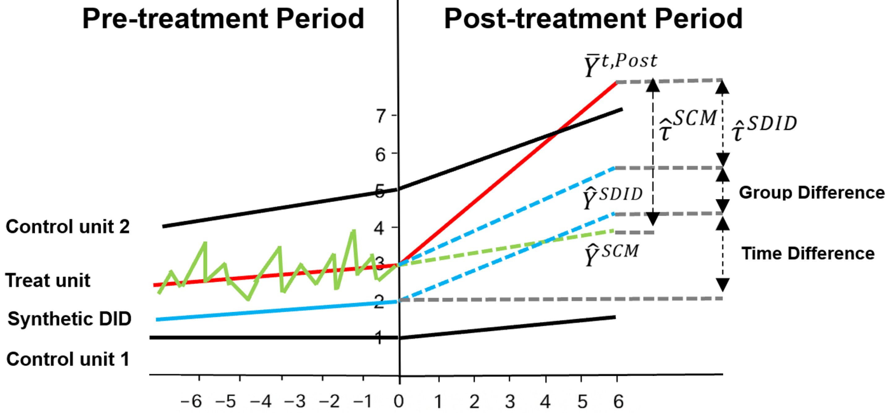
2.2. Synthetic Difference-in-Differences (SDID) Approach

The SDID approach introduced by Arkhangelsky et al. is an extension of the SCM [28]. The SCM could produce biased estimates due to the imperfect overlap in pretreatment periods. SDID addresses the identification challenges posed by the traditional DID method and mitigates the issue of imperfect overlap in pretreatment periods encountered in the SCM using both unit-specific weights and time-specific weights. Figure 1 demonstrates an example of mismatched pre-LCD periods. The absence of overlap between the green (SCM counterfactual) and red (Treatment unit) lines potentially leads to biased estimates. By assigning greater weights to the most recent pre-LCD periods, SDID can effectively minimize the bias of the time trends among the counterfactual and the treatment unit surrounding the implementation timing. Figure 1 also demonstrates the SDID counterfactual running parallel to the trend of the treatment unit in the pre-LCD periods, thereby reducing the bias associated with the SCM.

In this study, we have a balanced panel with 41 cities and 120 days (1 February–31 May). T_pre represents the pre-LCD periods (1 February–25 March), while T_post represents the 2022 LCD periods (26 March–31 May). N_co denotes the control units, including the remaining cities in the YRD region except Shanghai, and N_tr equals N − N_co, representing the treated unit (i.e., Shanghai). The weights ${{\widehat{\omega }}_n}^{SDID}$ align the trends in the untreated units with the pre-LCD trends in the treated unit. For example, ${\displaystyle {\sum }_{n=1}^{N_{co}}} {{\widehat{\omega }}_n}^{SDID}{Y}_{nt}\approx {N_{tr}}^{-1}{\displaystyle {\sum }_{n=N_{co}+1}^{N_{tr}}}{Y}_{nt}$ for t = 1, …, T_pre. The time weights of ${{\widehat{\lambda }}_t}^{SDID}$ minimize the gap between the pre-LCD and 2022 LCD periods for the control units. For example, ${\displaystyle {\sum }_{t=1}^{T_{pre}}} {{\widehat{\lambda }}_t}^{SDID} Y_{nt}\approx {T_{post} }^{-1}{\displaystyle {\sum }_{t=T_{pre}+1}^{T_{post}}}{Y}_{nt}$ for n = 1, …, N_co.

To estimate the causal relationship between the 2022 LCD and changes in O₃ concentrations, we specified the corresponding regression model for SDID as follows:

$$\left({\widehat{\tau }}^{SDID},\widehat{\mu },\widehat{\alpha },\widehat{\beta }\right)=argmin\left\{{\displaystyle {\sum }_{n=1}^N}{\displaystyle {\sum }_{t=1}^T}({Y_{nt}-\mu -{\alpha }_n-{\beta }_t-W_{nt}\tau )}^2{{\widehat{\omega }}_n}^{SDID}{{\widehat{\lambda }}_t}^{SDID}\right\}$$

(1)

where O₃ concentration for unit n in period t is denoted by $Y_{nt}$, and exposure to the 2022 LCD is denoted by $W_{nt}\in \left\{\mathrm{0,1}\right\}$. ${\alpha }_n$ and ${\beta }_t$ are unit-fixed effect and time-fixed effect, respectively. The weights of ${{\widehat{\omega }}_n}^{SDID}$ and ${{\widehat{\lambda }}_t}^{SDID}$ are used to calculate a weighted average of O₃ concentrations in the control units, simulating a comparable counterfactual O₃ concentration in Shanghai. This approach enables us to estimate the average treatment effect (ATE) of the 2022 lockdown, which refers to its impact on deweathered O₃ concentrations. The estimated effect is denoted by ${\widehat{\tau }}^{SDID}$. The “synthdid” R package was utilized in R version 4.4.3 to implement the SDID approach (https://synth-inference.github.io/synthdid, accessed on 15 March 2023). A comprehensive description of the methodology can be found in Arkhangelsky et al. [35].

In order to assess the causal impact of the 2022 LCD on O₃ concentration, the MDA8 O₃ concentration (hereafter O₃ unless specified) in Shanghai was designated as the treatment unit, while the O₃ concentration in the remaining 40 cities in the YRD region served as the control units. The selection criteria for control units in the SDID model include the following factors: (1) the absence of similar interventions to the 2022 LCD, (2) no significant idiosyncratic shocks to the O₃ concentration during the 2022 LCD, and (3) similarity to Shanghai in relevant characteristics such as emission levels and meteorological conditions. Following the methodology outlined by Abadie et al., we backdated the intervention date to 26 March 2022, two days before the official announcement (28 March 2022) of the lockdown to account for the possibility of an anticipation effect on local air pollution levels [39]. We also implemented a pre-intervention duration from 1 February to 25 March 2022 to ensure a sufficient pretreatment period.

To check the robustness of the main empirical results, we implemented a placebo test by introducing simulated starting lockdown dates and hypothetical treatment units. Subsequently, we conducted this test while excluding geographically adjacent regions susceptible to the influence of Shanghai’s 2022 lockdown.

2.3. Estimating the Health Impact and Economic Costs

The estimation of total premature mortalities attributable to elevated O₃ concentration exposure in Shanghai during 2022 LCD is calculated based on the following widely used exposure–response functions:

$$RR=\exp \left[\beta \times \left(C-C_0\right)\right]$$

(2)

$$∆M=f_p\times P\times \left[\right(RR-1)∕RR]$$

(3)

where β is the exposure–response coefficient, with values derived from the long-term epidemiological study by Turner et al. and cardiovascular and respiratory mortality by Lim et al. [40,41]. For an increase of 10 μg/m³ in O₃ concentration, the β value was determined as 0.29% (95% CI: 0.1 to 0.5%) for cardiovascular disease, 0.39% (95% CI: 0 to 0.86%) for respiratory disease, and 0.19% (95% CI: 0.1% to 0.39%) for all-cause mortality (

Table 1. The long-term exposure–response coefficient (β), RR, and baseline mortality for ozone (10 μg/m³).

Parameter	All-Cause (95% CI)	Cardiovascular (95% CI)	Respiratory (95% CI)
β (O3)	0.00198	0.00296	0.00392
	(0.001, 0.00392)	(0.001, 0.00583)	(0, 0.00862)
RR (O3)	1.0221	1.0197	1.0262
	(1.0066, 1.0262)	(1.0066, 1.0393)	(1.0066, 1.0586)
p (O3)	0.00654	0.00296	0.00072

). The exposed O₃ concentration C represents the deweathered concentration, whereas C₀ denotes the minimum risk exposure level, which is set at 26.7 ppb [40]. Equation (2) calculates the relative risk (RR) of cardiovascular and respiratory disease mortalities, along with a 95% confidence interval [42,43,44,45]. ∆M represents the number of premature deaths resulting from elevated O₃ concentration; f_p denotes the baseline incidence rate obtained from the China Health Statistical Yearbook 2022 compiled by the National Health Commission of the People’s Republic of China (http://www.nhc.gov.cn, accessed on 17 May 2023); P denotes the population data of Shanghai obtained from the website of the Shanghai Municipal Bureau of Statistics (https://tjj.sh.gov.cn, accessed on 6 February 2023). More details for the parameters used in Equations (2) and (3) can be found in a previous study [43]. We first estimated premature mortality attributed to O₃ exposures throughout the 2022 LCD using deweathered O₃ concentrations in Shanghai. Subsequently, this concentration undergoes an adjustment using the O₃ concentrations in synthetic Shanghai from the SDID model, representing the average O₃ concentration under the assumption of no lockdown. The differences in the premature mortality estimated based on these two O₃ concentrations (observed and adjusted) are considered premature deaths associated with the 2022 LCD.

The value of statistical life (VSL) has been used to evaluate the economic costs of O₃ exposure mortalities [46,47]. It serves as a monetary measure reflecting individuals’ willingness to pay to prevent diseases caused by elevated ozone concentration. In this study, we applied the benefits transfer method to estimate the city-specific VSL from Shanghai by adjusting the per capita GDP and price index. VSL is affected by factors such as individual income levels and inflation rates in different years. The Shanghai VSL per person in 2022 can be represented by Equation (4) [48,49]:

$${VSL}_{TY}={VSL}_{BY}\times {\displaystyle \frac{{CPI}_{TY}}{{CPI}_{BY}}}\times ({\displaystyle \frac{{Income}_{TY}}{{Income }_{BY}}}{)}^e$$

(4)

The VSL was obtained from Wang & Ge, where VSL_BY represents the VSL_TY value of Shanghai in 2017, CPI_BY and CPI_TY denote the Consumer Price Index in 2017 and 2021, respectively, while Income_BY and Income_TY denote the per capita disposable annual income in 2017 and 2021, respectively [50]. The income elasticity e, assumed to be 0.8 as recommended by the Organization for Economic Co-Operation and Development (OECD), was also considered [51]. The following equation calculates the corresponding economic costs associated with increased premature deaths:

$$\Delta E=\Delta M \times { VSL}_{TY}$$

(5)

where ΔE represents the economic costs, ΔM denotes the number of increased premature deaths from Equation (3), and VSL_TY is the outcome of Equation (4).

3. Results

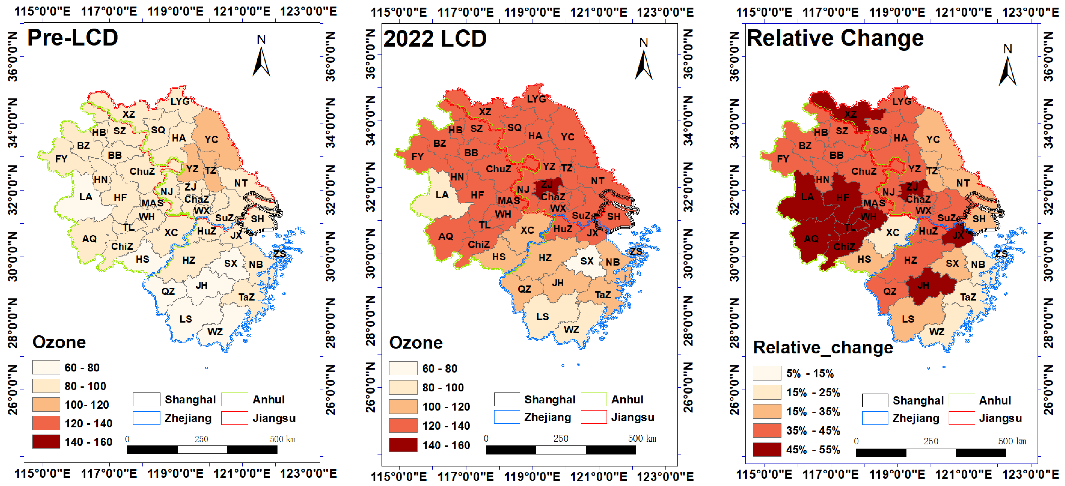
3.1. Overview of Air Quality Changes During the 2022 LCD

Table 2. Summary statistics of key variables.

Variable	Shanghai			Remaining YRD Region Cities			Mean Diff.
	Pre- LCD	2022 LCD	Relative Change	Pre- LCD	2022 LCD	Relative Change	Pre- LCD	2022 LCD
MDA8 O3 (μg/m3)	93.2 ± 17.6	123.8 ± 29.3	32.8%	88.9 ± 27.5	123.6 ± 35.7	39.0%	4.3	0.2
NO2 (μg/m3)	30.7 ± 11.8	17.2 ± 6.3	−44.0%	26.2 ± 12.2	21.7 ± 9.3	−17.2%	4.5 **	−4.5 ***
CO (mg/m3)	0.6 ± 0.1	0.7 ± 0.1	16.7%	0.6 ± 0.2	0.5 ± 0.1	−11.3%	0	0.2 ***
PM10 (μg/m3)	48.7 ± 28.2	33.3 ± 17.0	−31.6%	67.2 ± 41.2	53.6 ± 21.1	−20.2%	−18.5 ***	−20.3 ***
PM2.5 (μg/m3)	30.0 ± 17.6	20.6 ± 10.3	−31.3%	38.4 ± 21.2	28.1 ± 11.7	−26.8%	−8.4 ***	−7.5 ***
SO2 (μg/m3)	5.6 ± 1.4	6.3 ± 1.6	14.3%	7.1 ± 2.6	7.5 ± 2.7	5.6%	−1.5 ***	−1.2 ***
Temperature (°C)	12.6 ± 6.53	22.2 ± 4.9	76.2%	12.4 ± 7.29	22.8 ± 5.5	83.9%	0.2	−0.6
Wind speed (m/s)	0.2 ± 0.1	0.2 ± 0.1	−0.3%	0.7 ± 0.7	0.6 ± 0.6	−14.3%	−0.5 ***	−0.4 ***
Relative humidity (%)	72.2 ± 13.5	70.4 ± 16.6	−2.5%	72.3 ± 15.5	67.9 ± 14.8	−6.1%	−0.1	2.5
Pressure (hPa)	1022.5 ± 7.0	1015.5 ± 6.3	−0.7%	1022.2 ± 7.2	1014.9 ± 6.4	−0.7%	0.3	0.6

Notes: The significance of the mean difference is calculated from the t-test. *, ** and *** denote significance levels of 10%, 5% and 1%.

presents the MDA8 O₃, NO₂, CO, PM_2.5, PM₁₀, and SO₂ concentrations from 1 February to 31 May 2022 for the 41 YRD cities, divided into two groups: Shanghai and the remaining cities. Both groups showed significant NO₂, PM₁₀, and PM_2.5 drops during the 2022 LCD compared to those in the pre-LCD periods. The concentrations of NO₂, PM₁₀, and PM_2.5 in Shanghai decreased by as much as 13.5 μg/m³ (relative change of 44.0%), 15.4 μg/m³ (31.6%), and 9.4 μg/m³ (31.3%), respectively. CO and SO₂ increased by 16.7% and 14.3%, while the MDA8 O₃ increased significantly by 32.8% in Shanghai. To further assess comparability, we calculated the mean differences between Shanghai and the remaining YRD region cities in key variables and conducted two-sample t-tests. Table 2 shows that, except for wind speed, the differences are not statistically significant in MDA8 O₃ concentrations and meteorological variables (temperature, relative humidity, pressure). This supports our assumption that Shanghai and the selected control cities are similar in terms of emissions and meteorological conditions.

Increased O₃ concentration during the 2022 LCD period was also observed across the entire YRD (Figure 2), with a relative increase ranging from 7.7% (Zhoushan in Zhejiang province) to 51.8% (Hefei in Anhui province) at the city level. The much higher temperatures during the 2022 LCD periods (up by 76.2% in Shanghai and 83.9% for the remaining cities) led to more favorable meteorological conditions for ozone formation, thus imposing challenges in disentangling the causal effects of policy measures. Elevated O₃ concentration was mainly observed over western Jiangsu, northern Zhejiang, and eastern Anhui province. These urban areas are known to have significant geographical proximity to Shanghai. However, despite their close geographical ties, they exhibited diverse responses to O₃ levels among the YRD cities. Compared to the observed values, the deweathered O₃ concentrations increased by ~40% during the 2022 LCD, compared to the pre-LCD (Figure S2). This variation may be attributed to both natural and anthropogenic factors, including differing weather patterns, local industrial activities, and traffic patterns during the 2022 lockdown [52,53,54].

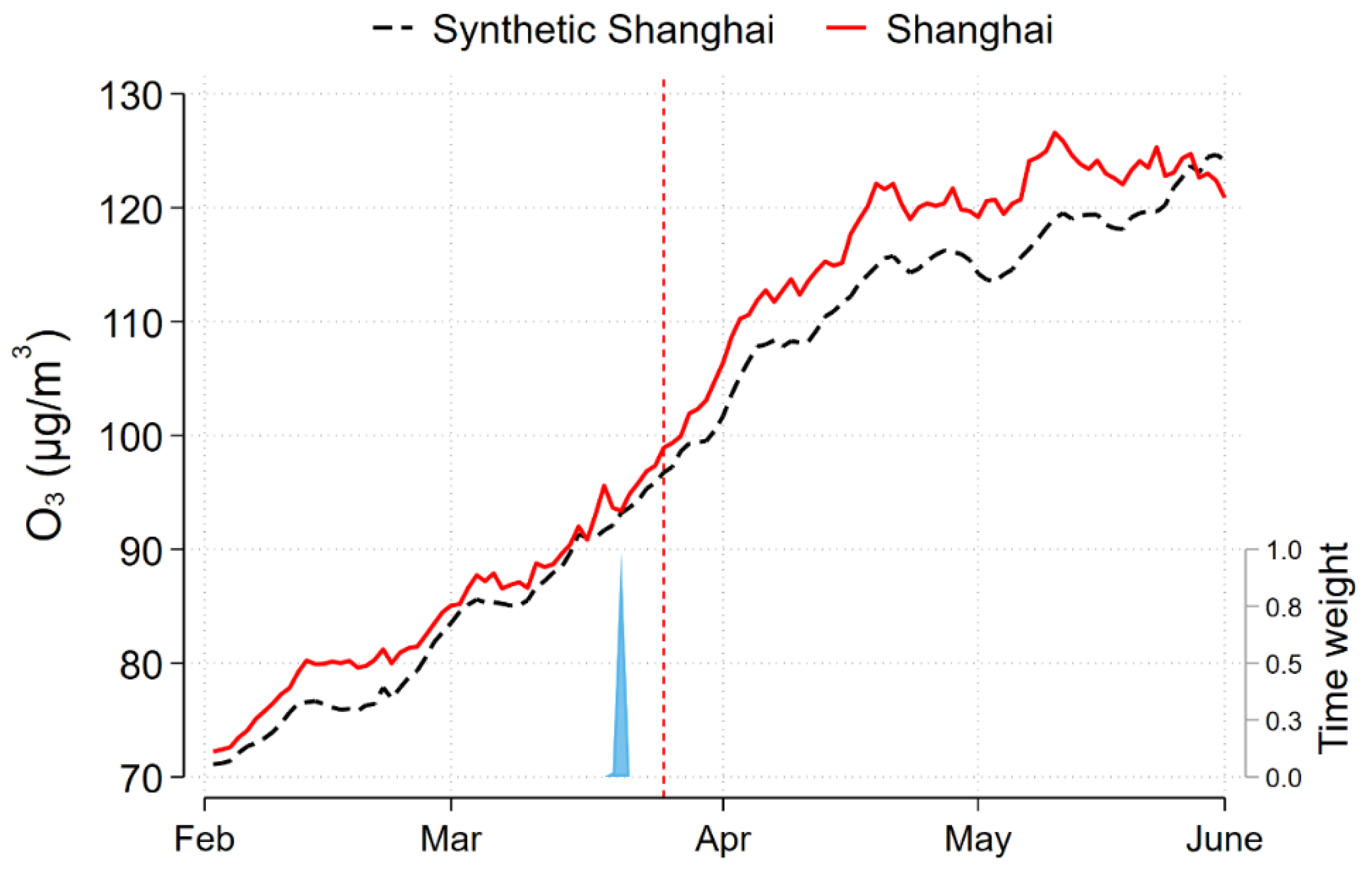
3.2. Causal Impact of Lockdown on Ozone

Figure 3 presents the deweathered O₃ concentrations in Shanghai and the synthetic Shanghai. As demonstrated in Figure 3, the deweathered O₃ concentration in Shanghai still shows an increasing trend, mostly due to temperature increase, and exhibits a more rapid growth trajectory after implementing the lockdown policy. The discrepancy between the real Shanghai and the synthetic Shanghai displayed a continuous expansion until approximately one week before the official lifting date of the lockdown. Subsequently, a gradual diminishment of this gap occurred, eventually leading to an overlapping pattern. This phenomenon coincided with Shanghai’s phased adjustment of containment measures, which included categorizing residential units into three distinct zones: lockdown areas, controlled areas, and prevention areas [55]. Such a transition suggested a phased return to pre-pandemic conditions as the overall epidemiological situation eased, with Shanghai progressively resuming normal economic activities towards the end of May.

Table 3. SDID regression results.

	Whole LCD		One Week Earlier
	(1) w/o Covariates	(2) With Covariates	(3) w/o Covariates	(4) With Covariates
ATT	3.5	3.7 *	4.0 *	4.4 **
	(2.35)	(2.26)	(2.30)	(2.12)
p value	0.13	0.09	0.08	0.04
95% CI	(−1.09, 8.09)	(−0.72, 8.12)	(−0.49, 8.49)	(0.24, 8.56)
Covariates	No	Yes	No	Yes
Time FE	Yes	Yes	Yes	Yes
City FE	Yes	Yes	Yes	Yes
N	4920	4920	4633	4633

Notes: Robust standard errors clustered at the city level are reported in parentheses. * and ** denote significance levels of 10% and 5%.

summarizes the causal impacts of lockdown on O₃ concentration under different specifications. Columns (1) and (2) present SDID estimates for the average treatment effect on treated city (ATT), both without and with covariates, yielding values of 3.5 (95% CI: −1.09–8.09) μg/m³ and 3.7 (95% CI: −0.72–8.12) μg/m³, respectively, which corresponds to a 3.8% and 4.0% increase relative to the pre-lockdown mean. The former is statistically insignificant, while the latter is statistically significant at the 10% level. Considering the resumption of production at the end of May, we opted for an endpoint of 24 May 2022, a week earlier than the official lifting date. We re-evaluated the causal effect of the 2022 LCD. Columns (3) and (4) show the SDID estimates for the average treatment effect, again without and with covariates, resulting in values of 4.0 (95% CI: −0.49–8.49) μg/m³ and 4.4 (95% CI: 0.24–8.56) μg/m³, respectively, which corresponds to a 4.2% and 4.7% increase relative to the pre-lockdown mean. The former is statistically significant at the 10% level, whereas the latter is at the 5% level. Among the four specifications, the estimate in Column (4) is considered the most informative, as it incorporates a comprehensive set of covariates and aligns the intervention window more accurately with the actual timeline of economic reopening. These refinements enhance the internal validity of the estimation. This result exhibits a positive effect that is statistically significant at the 5% level. In short, our calculation suggests a 4.4 μg/m³ increase in O₃ concentration in Shanghai following the implementation of the 2022 LCD.

We assessed the validity of our findings through a series of robustness checks (

Table 4. Robustness checks.

	In-Time Placebo		In-Place Placebo		Spillover Effect		Alternative Method
	(1)	(2)	(3)	(4)	(5)	(6)	(7)
	Stage 0	Stage 1	Top 5	Top 10	Border 1	Border 2	SCM
ATT	−4.3	4.1	−2.2	−2.0	4.8 *	5.2 *	4.6 ***
	(4.88)	(3.77)	(1.44)	(1.36)	(2.56)	(2.60)	(2.05)
p value	0.38	0.28	0.13	0.14	0.06	0.05	0.01
95% CI	(−13.86, 5.26)	(−3.30, 11.50)	(−5.03, 0.63)	(−4.67, 0.67)	(−0.23, 9.83)	(0.10, 10.30)	(0.59, 8.61)
N	4633	4633	4520	4520	4181	3164	4633

Notes: Robust standard errors clustered at the city level are reported in parentheses; *, ** and *** denote significance levels of 10%, 5% and 1%.

). There has been debate regarding the temporal implementation of the 2022 LCD. In response to curbing the rapid spread of the Omicron variant, the Shanghai government introduced a series of public health and social measures. Stage 0, representing the period of regular COVID-19 prevention and control measures from 1 March to 13 March, mirrored the measures in place during 2021 [56]. In Stage 1, passenger stations ceased operations from 14 March onwards [57]. Subsequently, in Stage 2, a “static management” lockdown was enforced in the city’s eastern half starting on 28 March [58]. To validate the robustness of our baseline findings, we followed the methodology of Abadie et al. and conducted placebo tests, including both in-time and in-place placebo analyses [26]. These tests are designed to ensure that our estimated treatment effects are not driven by random chance or unobserved confounding factors. Firstly, for the in-time placebo test, we simulated the lockdown intervention at two earlier dates—Stage 0 (1 March) and Stage 1 (14 March)—when no official lockdown had been implemented in Shanghai or other YRD cities. The same model specifications and estimation procedures were used as in the main analysis. If MDA8 O₃ concentrations had shown significant increases during these placebo periods, it would indicate that the observed effects in our baseline estimates may be driven by other confounding factors rather than the actual lockdown. As we expect, the results in cases (1) and (2) reveal that the causal effects become statistically insignificant during the absence of strict lockdown measures in Stages 0 and 1.

Secondly, we performed an in-place placebo test by selecting the top five and top ten cities that contributed most to the construction of synthetic Shanghai (Figure S3). These cities were assigned as simulated treatment units, while the remaining YRD cities served as controls. Using the same model settings and code as the main analysis, we estimated the effect of a hypothetical 2022 LCD in these cities. Since no lockdown occurred outside Shanghai, we would not expect any significant effects. Indeed, Cases (3) and (4) showed negative and statistically insignificant results, confirming that our main findings are not driven by chance.

Moreover, to address the potential issue of spillover effects, neighboring cities close to Shanghai may have experienced indirect impacts from the lockdown, such as reductions in intercity traffic or economic activity [59]. We also constructed new control units by eliminating border cities that share a boundary with Shanghai, including Nantong, Suzhou, Jiaxing, and Ningbo, to mitigate the potential confounding effects stemming from the spillover effect. Furthermore, cities sharing a boundary with the previously excluded border cities, like Yancheng, Taiizhou, Changzhou, Wuxi, Huzhou, Hangzhou, Shaoxing, Taizhou, and Zhoushan, were also omitted from the analysis. Cases (5) and (6), which exclude border cities potentially affected by spillover effects, show a larger increase in deweathered O₃ concentrations—4.8 (95%CI: 0.23–9.83) µg/m³ and 5.2 (95%CI: 0.10–10.30) µg/m³, respectively. These stronger effects suggest that the baseline estimates may have been biased downward due to spillover from the 2022 LCD into neighboring control cities. This reinforces the conclusion that the lockdown had a substantial and positive impact on O₃ concentration.

Lastly, as an alternative to the SDID, we conduct a synthetic control method to revalidate our results with the SDID ones (Figure S4). In case (7), we present an SCM estimate of 4.6 (95%CI: 0.59–8.61) µg/m³, which attains statistical significance at the 1% level. The above findings demonstrate the robustness of our results regarding the influence of the 2022 LCD on deweathered O₃ concentration.

3.3. Health Impact and Economic Costs Due to Short-Term Ozone Exposure

The estimated results (Figure S5) indicate that during the 2022 LCD period, a total of 380 (95% CI: 193–748) premature mortalities are attributed to O₃ exposure. Cardiovascular and respiratory diseases account for 45.3% and 11.1% of the total premature mortality, respectively. If no lockdown occurs, O₃ levels are expected to decrease by an average of 4.4 μg/m³ based on the SDID results. The total O₃-related premature mortality is expected to be 356 (95% CI: 180–700), representing a 7.0% decrease. A comparison of premature mortality between the observed and simulated scenarios reveals an estimated increase of 24 premature deaths due to the lockdown, constituting 6.3% of the expected premature mortality during the 2022 LCD. The estimated economic damages during the 2022 LCD were 12.8 million USD, 5.8 million USD, and 1.6 million USD for all-cause, cardiovascular, and respiratory diseases, respectively.

Table 5. Premature mortality and economic influence related to long-term exposure to air pollutants around the world due to the COVID-19 lockdown.

Pollutants	Reference	Year	Country (City)	Premature Mortality	Economic Influence (USD)
O3	Ye et al. [63]	2020	China	215	0.95 billion
PM2.5	Wang & Ge [50]	2022	China (YRD)	35,342	18.86 billion
	Seo et al. [60]	2020	Korea (Seoul)	250	884 million
	Kumar et al. [61]	2020	India	630	0.69 billion
	Leão et al. [62]	2021	Brazil (Recife)	164	294 million
	Li et al. [16]	2020	China (YRD)	42,400	/
	Cole et al. [27]	2020	China	50,800	/

presents the health and economic influence of long-term exposure to O₃ and PM_2.5 during the COVID-19 lockdown period in various countries and cities worldwide [16,27,50,60,61,62,63]. For instance, in 2020, China experienced 215 potential premature deaths related to O₃ exposure, resulting in economic costs of 0.95 billion USD. In 2022, the YRD region recorded 35,342 avoided premature deaths due to a reduction of PM_2.5, contributing to economic benefits of 18.86 billion USD.

3.4. Limitation of Synthetic Difference-in-Differences

While the synthetic difference-in-differences (SDID) method provides a robust framework for causal inference, it also has limitations that may affect its applicability in certain contexts [28,59]. First, constructing a synthetic control requires assigning weights to donor units (i.e., control cities) to match the treated unit’s pre-treatment trend. The selection of the donor pool can significantly influence the results, and there is no universally accepted criterion for this process. As a result, subjective judgment in choosing donor units may affect the transparency and replicability of the analysis. Second, SDID performs best in stable policy environments. When multiple interventions occur simultaneously or policies change dynamically, it becomes challenging to disentangle the effect of a single intervention, potentially biasing the estimates. Third, the method relies on the assumption that the treated and control groups are comparable in characteristics and pre-treatment trends. If substantial differences exist—for example, in emissions profiles or meteorological conditions—the synthetic control may fail to approximate a credible counterfactual, weakening the validity of the results.

Therefore, researchers must carefully evaluate the context-specific suitability of the SDID approach. Key considerations include the appropriateness of the donor pool, the stability and timing of policy implementation, and the degree of similarity between treatment and control groups. Addressing these issues through robustness checks and transparent methodological choices is essential to ensure the credibility and validity of the findings.

4. Conclusions and Future Study

Short-term emission changes—whether arising from natural phenomena or anthropogenic activities—can substantially influence air quality. The prompt and accurate evaluation of these impacts is essential for safeguarding public health and guiding effective environmental management strategies. This study demonstrates that the two-step synthetic difference-in-differences (SDID) approach provides a robust, data-driven, and cost-effective framework for identifying the causal impacts of such short-term emission changes. Using the 2022 Shanghai lockdown as a natural experiment, we find a statistically significant increase in deweathered MDA8 O₃ concentrations, with an average rise of 4.4 μg/m³ (significant at the 5% level; 95% CI: 0.24–8.56). Rigorous placebo tests—including both in-time and in-place simulations—support the credibility of these findings and help rule out confounding factors or spurious correlations. Importantly, we also quantify the associated health burden: our estimates suggest that the lockdown-induced O₃ increase may have led to approximately 24 additional premature deaths (95% CI: 13–48) in Shanghai, with an economic cost of roughly 12.8 million USD. This integrative framework not only enhances our understanding of the unintended consequences of large-scale public health interventions but also serves as a practical tool for policymakers to design more balanced and targeted emission control measures.

Looking forward, future studies could expand the application of SDID to other pollutants (e.g., PM_2.5, NO₂), diverse urban settings, or different types of policy shocks (e.g., industrial shutdowns, transportation bans). Furthermore, incorporating high-resolution population exposure data and long-term health outcomes could provide a more holistic picture of the societal impacts of short-term emission fluctuations.

References

1. Liang, Y.; Sengupta, D.; Campmier, M.J.; Lunderberg, D.M.; Apte, J.S.; Goldstein, A.H. Wildfire smoke impacts on indoor air quality assessed using crowdsourced data in California. Proc. Natl. Acad. Sci. USA 2021, 118, e2106478118. [Google Scholar] [CrossRef]
2. Schneider, S.R.; Lee, K.; Santos, G.; Abbatt, J.P.D. Air Quality Data Approach for Defining Wildfire Influence: Impacts on PM2.5, NO2, CO, and O3 in Western Canadian Cities. Environ. Sci. Technol. 2021, 55, 13709–13717. [Google Scholar] [CrossRef] [PubMed]
3. Ghetu, C.C.; Rohlman, D.; Smith, B.W.; Scott, R.P.; Adams, K.A.; Hoffman, P.D.; Anderson, K.A. Wildfire Impact on Indoor and Outdoor PAH Air Quality. Environ. Sci. Technol. 2022, 56, 10042–10052. [Google Scholar] [CrossRef] [PubMed]
4. Zhou, Y.; Wu, Y.; Yang, L.; Fu, L.; He, K.; Wang, S.; Hao, J.; Chen, J.; Li, C. The impact of transportation control measures on emission reductions during the 2008 Olympic Games in Beijing, China. Atmos. Environ. 2010, 44, 285–293. [Google Scholar] [CrossRef]
5. Zhang, G.; Xu, H.; Wang, H.; Xue, L.; He, J.; Xu, W.; Qi, B.; Du, R.; Liu, C.; Li, Z.; et al. Exploring the inconsistent variations in atmospheric primary and secondary pollutants during the 2016 G20 summit in Hangzhou, China: Implications from observations and models. Atmos. Chem. Phys. 2020, 20, 5391–5403. [Google Scholar] [CrossRef]
6. Zhu, W.; Hu, B.; Liu, Z.; Pan, Y.; Han, J.; Li, C.; Xu, M.; Yang, S.; Yin, Y.; Zhou, J.; et al. Reduction of anthropogenic emissions enhanced atmospheric new particle formation: Observational evidence during the Beijing 2022 Winter Olympics. Atmos. Environ. 2023, 314, 120094. [Google Scholar] [CrossRef]
7. Wang, S.; Zhao, M.; Xing, J.; Wu, Y.; Zhou, Y.; Lei, Y.; He, K.; Fu, L.; Hao, J. Quantifying the Air Pollutants Emission Reduction during the 2008 Olympic Games in Beijing. Environ. Sci. Technol. 2010, 44, 2490–2496. [Google Scholar] [CrossRef]
8. Xu, W.; Liu, X.; Liu, L.; Xin, J.; Wang, L.; Münkel, C.; Mao, G.; Wang, Y. Impact of emission controls on air quality in Beijing during APEC 2014: Implications from water-soluble ions and carbonaceous aerosol in PM2.5 and their precursors. Atmos. Environ. 2019, 210, 241–252. [Google Scholar] [CrossRef]
9. Ma, Y.; Fu, T.M.; Tian, H.; Gao, J.; Hu, M.; Guo, J.; Zhang, Y.; Sun, Y.; Zhang, L.; Yang, X.; et al. Emergency Response Measures to Alleviate a Severe Haze Pollution Event in Northern China During December 2015: Assessment of Effectiveness. Aerosol Air Qual. Res. 2020, 20, 2098–2116. [Google Scholar] [CrossRef]
10. Li, X.; Yao, Y.; Zhang, Z.; Zeng, Z.; Chen, Z.; Du, H. The health and economic impacts of emergency measures to combat heavy air pollution. J. Clean. Prod. 2023, 423, 138655. [Google Scholar] [CrossRef]
11. He, G.; Pan, Y.; Tanaka, T. The short-term impacts of COVID-19 lockdown on urban air pollution in China. Nat. Sustain. 2020, 3, 1005–1011. [Google Scholar] [CrossRef]
12. Dantas, G.; Siciliano, B.; França, B.B.; Da Silva, C.M.; Arbilla, G. The impact of COVID-19 partial lockdown on the air quality of the city of Rio de Janeiro, Brazil. Sci. Total Environ. 2020, 729, 139085. [Google Scholar] [CrossRef] [PubMed]
13. Grange, S.K.; Lee, J.D.; Drysdale, W.S.; Lewis, A.C.; Hueglin, C.; Emmenegger, L.; Carslaw, D.C. COVID-19 lockdowns highlight a risk of increasing ozone pollution in European urban areas. Atmos. Chem. Phys. 2021, 21, 4169–4185. [Google Scholar] [CrossRef]
14. Hashim, B.M.; Al-Naseri, S.K.; Al-Maliki, A.; Al-Ansari, N. Impact of COVID-19 lockdown on NO2, O3, PM2.5 and PM10 concentrations and assessing air quality changes in Baghdad, Iraq. Sci. Total Environ. 2021, 754, 141978. [Google Scholar] [CrossRef]
15. Jephcote, C.; Hansell, A.L.; Adams, K.; Gulliver, J. Changes in air quality during COVID-19 ‘lockdown’ in the United Kingdom. Environ. Pollut. 2021, 272, 116011. [Google Scholar] [CrossRef]
16. Li, Y.; Li, S.; Huang, L.; Liu, Z.; Zhu, Y.; Li, L.; Wang, Y.; Lv, K. The casual effects of COVID-19 lockdown on air quality and short-term health impacts in China. Environ. Pollut. 2021, 290, 117988. [Google Scholar] [CrossRef]
17. Liu, H.; Wang, C.; Zhang, M.; Wang, S. Evaluating the effects of air pollution control policies in China using a difference-in-differences approach. Sci. Total Environ. 2022, 845, 157333. [Google Scholar] [CrossRef]
18. Li, M.; Liu, H.; Geng, G.; Hong, C.; Liu, F.; Song, Y.; Tong, D.; Zheng, B.; Cui, H.; Man, H. Anthropogenic emission inventories in China: A review. Natl. Sci. Rev. 2017, 4, 834–866. [Google Scholar] [CrossRef]
19. Gao, M.; Han, Z.; Liu, Z.; Li, M.; Xin, J.; Tao, Z.; Li, J.; Kang, J.-E.; Huang, K.; Dong, X.; et al. Air quality and climate change, Topic 3 of the Model Inter-Comparison Study for Asia Phase III (MICS-Asia III)—Part 1: Overview and model evaluation. Atmos. Chem. Phys. 2018, 18, 4859–4884. [Google Scholar] [CrossRef]
20. Skipper, T.N.; Hu, Y.; Odman, M.T.; Henderson, B.H.; Hogrefe, C.; Mathur, R.; Russell, A.G. Estimating US Background Ozone Using Data Fusion. Environ. Sci. Technol. 2021, 55, 4504–4512. [Google Scholar] [CrossRef]
21. Wang, N.; Xu, J.; Pei, C.; Tang, R.; Zhou, D.; Chen, Y.; Li, M.; Deng, X.; Deng, T.; Huang, X.; et al. Air Quality During COVID-19 Lockdown in the Yangtze River Delta and the Pearl River Delta: Two Different Responsive Mechanisms to Emission Reductions in China. Environ. Sci. Technol. 2021, 55, 5721–5730. [Google Scholar] [CrossRef] [PubMed]
22. Callaway, B.; Sant’Anna, P.H.C. Difference-in-Differences with Multiple Time Periods. J. Econom. 2021, 225, 200–230. Available online: http://arxiv.org/abs/1803.09015 (accessed on 11 July 2023). [CrossRef]
23. Roth, J. Pretest with Caution: Event-Study Estimates After Testing for Parallel Trends. Am. Econ. Rev. Insights 2022, 4, 305–322. [Google Scholar] [CrossRef]
24. Abadie, A.; Gardeazabal, J. The Economic Costs of Conflict: A Case Study of the Basque Country. Am. Econ. Rev. 2003, 93, 113–132. [Google Scholar] [CrossRef]
25. Abadie, A.; Diamond, A.; Hainmueller, J. Synthetic Control Methods for Comparative Case Studies: Estimating the Effect of California’s Tobacco Control Program. J. Am. Stat. Assoc. 2010, 105, 493–505. [Google Scholar] [CrossRef]
26. Abadie, A.; Diamond, A.; Hainmueller, J. Comparative Politics and the Synthetic Control Method. Am. J. Political Sci. 2015, 59, 495–510. [Google Scholar] [CrossRef]
27. Cole, M.A.; Elliott, R.J.R.; Liu, B. The Impact of the Wuhan COVID-19 Lockdown on Air Pollution and Health: A Machine Learning and Augmented Synthetic Control Approach. Environ. Resour. Econ. 2020, 76, 553–580. [Google Scholar] [CrossRef]
28. Arkhangelsky, D.; Athey, S.; Hirshberg, D.A.; Imbens, G.W.; Wager, S. Synthetic Difference-in-Differences. Am. Econ. Rev. 2021, 111, 4088–4118. [Google Scholar] [CrossRef]
29. Li, G.; Fang, C.; Watson, J.E.; Sun, S.; Qi, W.; Wang, Z.; Liu, J. Mixed effectiveness of global protected areas in resisting habitat loss. Nat. Commun. 2024, 15, 8389. [Google Scholar] [CrossRef]
30. Wu, C.; Li, X.; Jiang, R.; Liu, Z.; Xie, F.; Wang, J.; Teng, Y.; Yang, Z. Understanding carbon resilience under public health emergencies: A synthetic difference-in-differences approach. Sci. Rep. 2024, 14, 20581. [Google Scholar] [CrossRef]
31. Chen, K.; Zhou, L.; Chen, X.; Bi, J.; Kinney, P.L. Acute effect of ozone exposure on daily mortality in seven cities of Jiangsu Province, China: No clear evidence for threshold. Environ. Res. 2017, 155, 235–241. [Google Scholar] [CrossRef]
32. Lu, X.; Hong, J.; Zhang, L.; Cooper, O.R.; Schultz, M.G.; Xu, X.; Wang, T.; Gao, M.; Zhao, Y.; Zhang, Y. Severe Surface Ozone Pollution in China: A Global Perspective. Environ. Sci. Technol. Lett. 2018, 5, 487–494. [Google Scholar] [CrossRef]
33. Chen, K.; Wang, P.; Zhao, H.; Wang, P.; Gao, A.; Myllyvirta, L.; Zhang, H. Summertime O3 and related health risks in the north China plain: A modeling study using two anthropogenic emission inventories. Atmos. Environ. 2021, 246, 118087. [Google Scholar] [CrossRef]
34. Wang, Y.; Wild, O.; Ashworth, K.; Chen, X.; Wu, Q.; Qi, Y.; Wang, Z. Reductions in crop yields across China from elevated ozone. Environ. Pollut. 2022, 292, 118218. [Google Scholar] [CrossRef] [PubMed]
35. Grange, S.K.; Carslaw, D.C.; Lewis, A.C.; Boleti, E.; Hueglin, C. Random forest meteorological normalisation models for Swiss PM 10 trend analysis. Atmos. Chem. Phys. 2018, 18, 6223–6239. [Google Scholar] [CrossRef]
36. Vu, T.V.; Shi, Z.; Cheng, J.; Zhang, Q.; He, K.; Wang, S.; Harrison, R.M. Assessing the impact of clean air action on air quality trends in Beijing using a machine learning technique. Atmos. Chem. Phys. 2019, 19, 11303–11314. [Google Scholar] [CrossRef]
37. Balogun, A.L.; Tella, A. Modelling and investigating the impacts of climatic variables on ozone concentration in Malaysia using correlation analysis with random forest, decision tree regression, linear regression, and support vector regression. Chemosphere 2022, 299, 134250. [Google Scholar] [CrossRef]
38. Huang, Q.; Li, T.; Zhang, T.; Fang, Y.; Gong, F.; Li, Y.; Xu, P.; Zhang, T.; Yang, L.; Wang, W. Quantifying SOA and O3 formation drivers in North China: Comprehensive method combining random forest, positive matrix factorization, and observation-based model. J. Environ. Sci. 2025, in press. [Google Scholar] [CrossRef]
39. Abadie, A. Using Synthetic Controls: Feasibility, Data Requirements, and Methodological Aspects. J. Econ. Lit. 2021, 59, 391–425. [Google Scholar] [CrossRef]
40. Turner, M.C.; Jerrett, M.; Pope, C.A.; Krewski, D.; Gapstur, S.M.; Diver, W.R.; Beckerman, B.S.; Marshall, J.D.; Su, J.; Crouse, D.L.; et al. Long-Term Ozone Exposure and Mortality in a Large Prospective Study. Am. J. Respir. Crit. Care Med. 2016, 193, 1134–1142. [Google Scholar] [CrossRef]
41. Lim, C.C.; Hayes, R.B.; Ahn, J.; Shao, Y.; Silverman, D.T.; Jones, R.R.; Garcia, C.; Bell, M.L.; Thurston, G.D. Long-Term Exposure to Ozone and Cause-Specific Mortality Risk in the United States. Am. J. Respir. Crit. Care Med. 2019, 200, 1022–1031. [Google Scholar] [CrossRef]
42. Huang, L.; Liu, Z.; Li, H.; Wang, Y.; Li, Y.; Zhu, Y.; Ooi, M.C.G.; An, J.; Shang, Y.; Zhang, D.; et al. The Silver Lining of COVID-19: Estimation of Short-Term Health Impacts Due to Lockdown in the Yangtze River Delta Region, China. GeoHealth 2020, 4, e2020GH000272. [Google Scholar] [CrossRef]
43. Zhang, X.; Cheng, C.; Zhao, H. A Health Impact and Economic Loss Assessment of O3 and PM2.5 Exposure in China from 2015 to 2020. GeoHealth 2022, 6, e2021GH000531. [Google Scholar] [CrossRef] [PubMed]
44. Feng, T.; Chen, H.; Liu, J. Air pollution-induced health impacts and health economic losses in China driven by US demand exports. J. Environ. Manag. 2022, 324, 116355. [Google Scholar] [CrossRef] [PubMed]
45. Li, X.B.; Fan, G. Interannual variations, sources, and health impacts of the springtime ozone in Shanghai. Environ. Pollut. 2022, 306, 119458. [Google Scholar] [CrossRef] [PubMed]
46. Ghude, S.D.; Chate, D.M.; Jena, C.; Beig, G.; Kumar, R.; Barth, M.C.; Pfister, G.G.; Fadnavis, S.; Pithani, P. Premature mortality in India due to PM2.5 and ozone exposure. Geophys. Res. Lett. 2016, 43, 4650–4658. [Google Scholar] [CrossRef]
47. Maji, K.J.; Ye, W.F.; Arora, M.; Nagendra, S.M.S. Ozone pollution in Chinese cities: Assessment of seasonal variation, health effects and economic burden. Environ. Pollut. 2019, 247, 792–801. [Google Scholar] [CrossRef]
48. Deschênes, O.; Greenstone, M.; Shapiro, J.S. Defensive Investments and the Demand for Air Quality: Evidence from the NOx Budget Program. Am. Econ. Rev. 2017, 107, 2958–2989. [Google Scholar] [CrossRef]
49. Wang, Y.; Sun, K.; Li, L.; Lei, Y.; Wu, S.; Jiang, Y.; Xi, Y.; Wang, F.; Cui, Y. Assessing the Public Health Economic Loss from PM2.5 Pollution in ‘2 + 26’ Cities. Int. J. Environ. Res. Public Health 2022, 19, 10647. [Google Scholar] [CrossRef]
50. Wang, Y.; Ge, Q. The positive impact of the Omicron pandemic lockdown on air quality and human health in cities around Shanghai. Environ Dev. Sustain. 2024, 26, 8791–8816. [Google Scholar] [CrossRef]
51. OECD Publishing. The Cost of Air Pollution: Health Impacts of Road Transport; OECD Publishing: Paris, France, 2014. [Google Scholar]
52. Liu, Y.; Wang, T.; Stavrakou, T.; Elguindi, N.; Doumbia, T.; Granier, C.; Bouarar, I.; Gaubert, B.; Brasseur, G.P. Diverse response of surface ozone to COVID-19 lockdown in China. Sci. Total Environ. 2021, 789, 147739. [Google Scholar] [CrossRef]
53. Deroubaix, A.; Brasseur, G.; Gaubert, B.; Labuhn, I.; Menut, L.; Siour, G.; Tuccella, P. Response of surface ozone concentration to emission reduction and meteorology during the COVID-19 lockdown in Europe. Meteorol. Appl. 2021, 28, e1990. [Google Scholar] [CrossRef]
54. Sicard, P.; De Marco, A.; Agathokleous, E.; Feng, Z.; Xu, X.; Paoletti, E.; Rodriguez, J.J.D.; Calatayud, V. Amplified ozone pollution in cities during the COVID-19 lockdown. Sci. Total Environ. 2020, 735, 139542. [Google Scholar] [CrossRef]
55. Hu, L.; Shi, M.; Li, M.; Ma, J. The effectiveness of control measures during the 2022 COVID-19 outbreak in Shanghai, China. PLoS ONE 2023, 18, e0285937. [Google Scholar] [CrossRef] [PubMed]
56. Tan, Y.; Wang, T. What caused ozone pollution during the 2022 Shanghai lockdown? Insights from ground and satellite observations. Atmos. Chem. Phys. 2022, 22, 14455–14466. [Google Scholar] [CrossRef]
57. Chen, Z.; Deng, X.; Fang, L.; Sun, K.; Wu, Y.; Che, T.; Zoua, J.; Cai, J.; Liu, H.; Wang, Y.; et al. Epidemiological characteristics and transmission dynamics of the outbreak caused by the SARS-CoV-2 Omicron variant in Shanghai, China: A descriptive study. Lancet Reg. Health—West. Pac. 2022, 29, 100592. [Google Scholar] [CrossRef] [PubMed]
58. Zhang, S.; Wang, S.; Xue, R.; Zhu, J.; He, S.; Duan, Y.; Huo, J.; Zhou, B. Impacts of Omicron associated restrictions on vertical distributions of air pollution at a suburb site in Shanghai. Atmos. Environ. 2023, 294, 119461. [Google Scholar] [CrossRef]
59. Cheng, N.; Zhang, W.; Xiong, T. Heterogenous impact of China’s place-based environmental regulations on its hog industry: A synthetic difference-in-differences approach. Can. J. Agric. Econ./Rev. Can. d’Agroecon. 2025, 73, 203–223. [Google Scholar] [CrossRef]
60. Seo, J.H.; Kim, J.S.; Yang, J.; Yun, H.; Roh, M.; Roh, M.; Yu, S.; Jeong, N.N.; Jeon, H.W.; Choi, J.S.; et al. Changes in Air Quality during the COVID-19 Pandemic and Associated Health Benefits in Korea. Appl. Sci. 2020, 10, 8720. [Google Scholar] [CrossRef]
61. Kumar, P.; Hama, S.; Omidvarborna, H.; Sharma, A.; Sahani, J.; Abhijith, K.V.; Debele, S.E.; Zavala-Reyes, J.C.; Barwise, Y.; Tiwari, A. Temporary reduction in fine particulate matter due to ‘anthropogenic emissions switch-off’ during COVID-19 lockdown in Indian cities. Sustain. Cities Soc. 2020, 62, 102382. [Google Scholar] [CrossRef]
62. Leão, M.L.P.; Penteado, J.O.; Ulguim, S.M.; Gabriel, R.R.; Santos, M.D.; Brum, A.N.; da Silva Júnior, F.M.R. Health impact assessment of air pollutants during the COVID-19 pandemic in a Brazilian metropolis. Environ. Sci. Pollut. Res. 2021, 28, 41843–41850. [Google Scholar] [CrossRef]
63. Ye, T.; Guo, S.; Xie, Y.; Chen, Z.; Abramson, M.J.; Heyworth, J.; Hales, S.; Woodward, A.; Bell, M.; Guo, Y.; et al. Health and related economic benefits associated with reduction in air pollution during COVID-19 outbreak in 367 cities in China. Ecotoxicol. Environ. Saf. 2021, 222, 112481. [Google Scholar] [CrossRef]
Figure 1. Illustration of the intuition behind SDID compared to SCM. The red line represents the treatment unit, while the two black lines depict the control units. The green line signifies the SCM counterfactual. The SDID method introduces time- and unit-specific weights, presenting the SDID counterfactual as the blue line.
Sustainability 17 06997 g001
Figure 2. City-level averaged MDA8 O3 concentrations during pre-LCD and 2022 LCD in the YRD region and the relative change (calculated as (2022 LCD—pre-LCD)/pre-LCD). Notes: The abbreviations represent various cities in the YRD region. AQ—Anqing; BB—Bengbu; BZ—Bozhou; ChaZ—Changzhou; Chiz—Chizhou; Chuz—Chuzhou; FY—Fuyang; HZ—Hangzhou; HF—Hefei; HA—Huaian; HB—Huaibei; HN—Huainan; HS—Huangshan; HuZ—Huzhou; JX—Jiaxing; JH—Jinhua; LYG—Lianyungang; LS—Lishui; LA—Luan; MAS—Maanshan; NJ—Nanjing; NT—Nantong; NB—Ningbo; QZ—Quzhou; SH—Shanghai; SX—Shaoxing; SQ—Suqian; SuZ—Suuzhou; SZ—Suzhou; TaZ—Taiizhou; TZ—Taizhou; TL—Tongling; WZ—Wenzhou; WH—Wuhu; WX—Wuxi; XC—Xuancheng; XZ—Xuzhou; YC—Yancheng; YZ—Yangzhou; ZJ—Zhenjiang; ZS—Zhoushan.
Sustainability 17 06997 g002
Figure 3. Estimated causal effects of the 2022 LCD on deweathered O3 concentration based on the SDID model. Notes: The solid straight red lines denote the deweathered data for the treated unit, Shanghai, while the dotted straight black lines represent unobserved counterfactual, synthetic Shanghai. The vertical dotted red line signifies the setting day of implementation of the 2022 LCD (26 March), and the shaded blue triangular area represents the time weights for each day before implementing the policy.
Sustainability 17 06997 g003