What Determines Carbon Emissions of Multimodal Travel? Insights from Interpretable Machine Learning on Mobility Trajectory Data

Abstract

Understanding the carbon emissions of multimodal travel—comprising walking, metro, bus, cycling, and ride-hailing—is essential for promoting sustainable urban mobility. However, most existing studies focus on single-mode travel, while underlying spatiotemporal and behavioral determinants remain insufficiently explored due to the lack of fine-grained data and interpretable analytical frameworks. This study proposes a novel integration of high-frequency, real-world mobility trajectory data with interpretable machine learning to systematically identify the key drivers of carbon emissions at the individual trip level. Firstly, multimodal travel chains are reconstructed using continuous GPS trajectory data collected in Beijing. Secondly, a model based on Calculate Emissions from Road Transport (COPERT) is developed to quantify trip-level CO₂ emissions. Thirdly, four interpretable machine learning models based on gradient boosting—XGBoost, GBDT, LightGBM, and CatBoost—are trained using transportation and built environment features to model the relationship between CO₂ emissions and a set of explanatory variables; finally, Shapley Additive exPlanations (SHAP) and partial dependence plots (PDPs) are used to interpret the model outputs, revealing key determinants and their non-linear interaction effects. The results show that transportation-related features account for 75.1% of the explained variance in emissions, with bus usage being the most influential single factor (contributing 22.6%). Built environment features explain the remaining 24.9%. The PDP analysis reveals that substantial emission reductions occur only when the shares of bus, metro, and cycling surpass threshold levels of approximately 40%, 40%, and 30%, respectively. Additionally, travel carbon emissions are minimized when trip origins and destinations are located within a 10 to 11 km radius of the central business district (CBD). This study advances the field by establishing a scalable, interpretable, and behaviorally grounded framework to assess carbon emissions from multimodal travel, providing actionable insights for low-carbon transport planning and policy design.

1. Introduction

The global urgency to mitigate greenhouse gas (GHG) emissions has made the decarbonization of urban transport systems a key priority in sustainable development agendas [1]. Urban areas account for approximately 75% of global energy consumption and nearly 80% of total GHG emissions, with the transportation sector alone contributing around 24% of global CO₂ emissions [2,3]. These figures continue to grow amid rapid urbanization and increasing demand for mobility. As cities expand and multimodal travel becomes more prevalent, understanding how individual travel behavior contributes to emissions is critical for designing effective low-carbon mobility strategies.

Substantial progress has been made in modeling transport-related carbon emissions, particularly through top-down and bottom-up estimation frameworks. These methods typically rely on aggregated data such as vehicle registrations, average trip lengths, or modal shares. While useful for macro-level analysis, existing models cannot effectively capture the temporal, spatial, and behavioral diversity of individual travel patterns in multimodal contexts, where a single trip may involve multiple transport modes, such as walking, cycling, metro, bus, and ride-hailing. Additionally, many models overlook low-emission segments, such as walking or public transit, or treat them simplistically due to inconsistent data availability and uncertainty in emission factors.

Traditional regression-based models struggle to reveal the non-linear interactions between built environment factors, modal combinations, and trip characteristics. Although machine learning (ML) techniques have demonstrated potential for predicting transport emissions, few studies use interpretable ML to explore how multimodal travel behaviors and spatial contexts jointly influence individual carbon footprints. The availability of high-resolution mobility data, such as GPS trajectories, opens new avenues for developing detailed, behaviorally informed emission models. These trajectory data enable the accurate reconstruction of travel paths, identification of modal transitions, and real-time emission calculations, offering clear advantages over aggregated or survey-based datasets [4].

However, most existing studies primarily focus on aggregated transportation emission estimates or single-mode analyses, lacking a nuanced understanding of emissions associated with individual-level multimodal travel behavior. Few systematically analyze the spatial–temporal structure of entire trips or the interplay between transport modes and built environment features. Consequently, assessing the impact of different modal combinations and urban contexts on individual carbon performance remains challenging.

To overcome these limitations, this study introduces a data-driven framework that leverages observed trajectory data and interpretable machine learning to evaluate carbon emissions from multimodal urban travel. This study aims to contribute to sustainable urban mobility by developing a data-driven framework to assess and reduce carbon emissions from multimodal travel, aligning with global sustainability goals to decarbonize urban transport systems. The main contributions are summarized as follows:

• It utilizes real-world, continuous trajectory data to integrate multimodal travel behavior and develops a carbon emission calculation method tailored to the carbon footprint of multimodal mobility.
• It applies interpretable machine learning techniques to identify key transportation behaviors and built environment factors that influence individual-level carbon emissions from multimodal travel, providing insights into the mechanisms behind low-carbon mobility decisions.

The remainder of this paper is organized as follows. Section 2 reviews the literature on estimating carbon emissions from urban transportation and the application of machine learning in this context. Section 3 introduces the data sources and the extraction of multimodal travel trajectories. Section 4 presents the Methodology, including the calculation of carbon emissions and the use of interpretable machine learning models. Section 5 reports the results and analysis. Section 6 concludes with key findings and policy implications. Section 7 discusses the study’s limitations and suggests directions for future research to enhance the robustness and generalizability of the findings.

2. Literature Review

This section reviews the relevant literature in two main areas: (1) methods and models used for estimating travel-related carbon emissions, and (2) studies exploring the determinants of travel emissions, including behavioral, spatial, and multimodal dimensions.

2.1. Estimation of Travel Carbon Emissions

Methods for estimating transport-related carbon emissions can be broadly categorized into top-down and bottom-up approaches [5,6]. Top-down methods rely on aggregated data, such as fuel sales, energy statistics, or national vehicle inventories, to estimate emissions at regional or national levels. While useful for macro-level assessments, they lack spatial or behavioral granularity.

In contrast, bottom-up methods estimate emissions at the trip, link, or segment level based on vehicle types, travel speeds, road classes, and emission factors. Among these, the COPERT model (Computer Programme to Calculate Emissions from Road Transport), developed by the European Environment Agency, is widely adopted for its transparency and adaptability. COPERT uses speed-dependent emission functions calibrated for various vehicle and fuel types. Though initially designed for European contexts, it has been successfully applied in Chinese cities such as Chengdu [7,8] and Shijiazhuang [9]. This is enabled by the technical equivalence between China’s emission standards and Euro standards, which supports the transferability of COPERT parameters to the Chinese context.

European studies have provided valuable methodological and empirical contributions to estimating emissions from multimodal transport. The TREMOVE model [10,11,12], developed by the European Commission, is widely used to simulate the long-term effects of transport policies—including modal shifts, pricing strategies, and vehicle technology transitions—on emissions and energy use across EU member states. Meanwhile, EU-wide travel surveys, such as Eurostat’s Harmonised Time Use Surveys and EU-SILC mobility modules, provide disaggregated data on individual trip behavior and modal combinations, supporting bottom-up emission estimation across diverse urban contexts.

In recent years, many researchers have also integrated trajectory data from taxis, ride-hailing, bike-sharing, and buses into bottom-up frameworks to achieve higher spatial–temporal resolution in emission modeling [13,14]. For instance, Shi et al. combined GPS data and COPERT emission factors to estimate ride-hailing emissions based on network centrality and traffic flow [15]. Liu et al. used taxi trajectories and urban GIS features to infer road-level emission hotspots [16]. However, most of these applications focus on single transport modes and do not fully capture the complexities of multimodal travel chains.

2.2. Determinants of Travel Carbon Emissions

Beyond emission estimation, an increasing number of studies seek to identify the key drivers of travel-related carbon emissions by examining both individual travel behavior and the attributes of the built environment. These investigations are crucial for informing the development of effective strategies to reduce travel-related carbon emissions.

Earlier studies predominantly employed statistical regression models to examine how factors such as income, trip length, and mode choice influence carbon emissions. Elements of the built environment have also been recognized as significant determinants. Drawing upon conceptual frameworks like the “5D model,” which encompasses Density, Diversity, Design, Destination Accessibility, and Distance to Transit, research has demonstrated that urban form substantially affects both travel mode selection and emission intensity. For instance, Handy et al. [17] found that a higher degree of land use mix and improved street connectivity were associated with reduced transportation emissions, primarily through increased use of active travel modes. However, these traditional modeling approaches often rely on assumptions of linearity and struggle to capture complex interactions or threshold effects.

Recent advances in machine learning (ML)—especially tree-based ensemble methods such as GBDT, XGBoost, and LightGBM—have enabled researchers to model complex, non-linear relationships in transport emissions. For example, Yu et al. applied six ML models to panel data from 254 Chinese cities and found that Extra-Trees and XGBoost performed best in predicting urban carbon emissions [18]. Zeng et al. introduced a graph-based learning framework to model transport emissions using OD flows and network structure [19].

However, most of these ML-based studies focus on predictive accuracy and neglect interpretability, which limits their value for policymaking. To address this, some researchers have begun integrating interpretable ML tools, such as SHAP (Shapley Additive Explanations) and PDPs (partial dependence plots). These methods facilitate a clearer understanding of how individual factors—such as modal shares, average travel speed, and land use diversity—influence predicted carbon emissions.

3. Data Preparation

3.1. Data Source and Description

This study analyzes multimodal travel behavior and associated carbon emissions using high-frequency GPS trajectory data collected by the Geolife project at Microsoft Research Asia between April 2007 and August 2012. The original dataset includes 17,621 GPS trajectories from 182 individuals, totaling approximately 1,292,951 km of recorded travel over 50,176 h.

A subset of 60 participants with mode-labeled mobility data in Beijing were selected for the case study. These participants represent a diverse urban population, including university students (58%), corporate employees (32%), and government staff (10%), with the majority aged between 22 and 30 years. Notably, 45% are between 22 and 26 years old, and 30% are between 26 and 30 years old. As shown in Figure 1a, university students constitute the largest group, followed by corporate employees and government staff. Their travel patterns are primarily concentrated within the Beijing metropolitan area, making the data particularly relevant for analyzing urban travel. The age distribution is presented in Figure 1b, indicating that most participants are between 22 and 30 years old.

While the dataset is limited to 60 participants from Beijing, primarily aged between 22 and 30, it holds considerable methodological value. The high-frequency, continuous GPS trajectory data, annotated with travel mode labels, serve as a rich and detailed source for reconstructing multimodal travel chains and estimating carbon emissions at the segment level. Although the data were collected between 2007 and 2012, they provide fine-grained, individual-level travel records across a wide range of modes—an asset that remains rare in urban mobility research. Their high spatial and temporal resolution supports both the development and validation of the proposed carbon emission profiling framework, while also facilitating interpretable machine learning analysis at the individual trip level.

3.2. Description of Individual Travel Data

The dataset comprises two main components: the trip dataset and the GPS trajectory dataset, which together support the reconstruction of multimodal travel behavior at an individual level.

• The trip dataset includes metadata such as user ID, trip ID, trip start and end times, origin and destination coordinates, and transportation mode labels. These labels were manually annotated by participants based on their actual travel modes. Modes include walking, biking, bus, metro, and private car.
• The GPS trajectory dataset records detailed spatial–temporal information for each trip, including timestamp, longitude, latitude, and instantaneous speed. Most data points were recorded at intervals of 1–5 s or 5–10 m, providing high-resolution tracking that is well-suited for identifying mode transitions and segmenting travel patterns.

To maintain focus on mode identification and carbon emission estimation, irrelevant variables such as altitude and total sampling duration were excluded from the analysis.

Table 1. Description of the trip dataset.

Field Name	Data Type	Example	Description
UserID	String	uxd7kLmn9pq2stv8wxy3zj	User identifier
TripID	String	ord5m8n2kxp7qrv4t9hwyc	Trip order ID
Start_Time	Datetime	15 June 2023 08:22:35	Start time of the trip
Start_Time	Datetime	15 June 2023 08:59:10	End time of the trip
Start_Location	geo_point	[113.256, 23.134]	Coordinates of origin
End_Location	geo_point	[113.389, 23.098]	Coordinates of destination
Type	String	bus	Mode of transport

(Source: Own elaboration based on the GeoLife dataset).

and

Table 2. Description of the GPS trajectory dataset.

Field Name	Data Type	Example	Description
OrderID	String	uxd7kLmn9pq2stv8wxy3zj	User identifier
TripID	String	ord5m8n2kxp7qrv4t9hwyc	Trip order ID
Timestamp	Datetime	15 June 2023 08:25:42	Timestamp
Longitude	Float	113.267892	Longitude
Latitude	Float	23.128456	Latitude
Speed	Float	4.2524	Instantaneous speed (m/s)

(Source: Own elaboration based on the GeoLife dataset).

describe the fields in the travel order and GPS trajectory datasets, respectively, which serve as the empirical foundation for reconstructing individual-level multimodal travel and modeling carbon emissions.

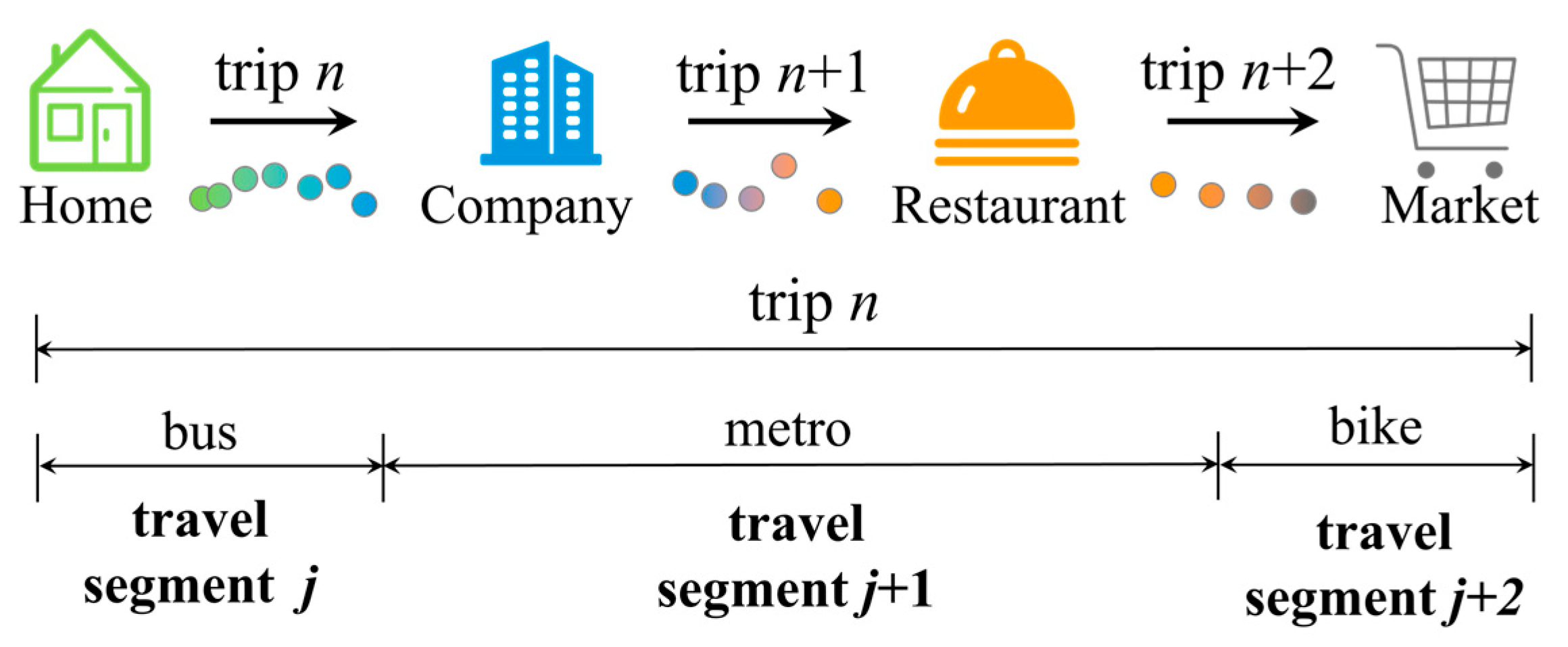
3.3. Data Extraction for Multimodal Travel

Multimodal travel refers to a sequence of spatial movements by an individual within the transportation system to complete one or more activities, involving the use of two or more distinct modes of transport. As shown in Figure 2, multimodal travel consists of multiple travel segments, each comprising a series of trajectory segments. Each trajectory segment corresponds to a single mode of transport.

To reconstruct accurate multimodal trip chains, we developed a systematic data fusion pipeline that integrates trip order records with high-frequency GPS trajectory data. Each trip order is associated with a unique OrderID and timestamp pair (start and end), which are used to extract the corresponding trajectory points from the GPS dataset.

Trajectory points are first filtered by temporal bounds (±2 min around the order time window) to account for potential recording delays. The trajectory segments are then sorted chronologically and matched to order records based on temporal overlap and spatial proximity between the order’s origin/destination and the GPS track’s start/end points. A dynamic time warping (DTW)-based similarity check is applied to validate the spatial–temporal alignment between each trajectory and its corresponding order segment.

To ensure segment continuity, we calculate inter-point time gaps and speed differentials. If the time gap between consecutive points exceeds 60 s or the instantaneous speed exceeds 60 m/s, the segment is flagged for interruption and excluded. Additionally, a minimum segment density threshold (1 point per 10 m) is enforced to filter low-resolution segments.

Outlier detection is performed using a combination of rule-based and statistical filters. Specifically, trajectory points are flagged as outliers if (i) their speeds exceed feasible human or vehicle thresholds (e.g., >5 km/h for walking, >20 km/h for cycling, >80 km/h for motorized modes), (ii) their bearing angle abruptly changes (>120° within 2 s), or (iii) they deviate >200 m from the expected path inferred by linear interpolation. These points are removed before segment assembly.

In cases of signal loss or abrupt GPS gaps, we interpolate missing points only when the time gap is under 30 s and the spatial gap is under 150 m, using linear interpolation to avoid distorting the route geometry. Otherwise, the segment is split at the gap boundary, and the resulting subsegments are re-evaluated for validity.

Following these steps, valid trajectory segments are merged with travel order metadata to form multimodal trip chains, each composed of mode-specific travel segments with consistent spatiotemporal attributes. This fusion process ensures both the high granularity and reliability of the reconstructed multimodal travel dataset.

Finally, validated multimodal trips are compiled per user, creating a comprehensive dataset of travel features for each participant. For the 60 volunteers, transportation mode labels (e.g., walking, biking, bus, car, metro) are assigned. Overall, 5180 travel segments are merged to create 1256 valid multimodal trips. This dataset provides a solid foundation for assessing carbon emissions within the context of multimodal travel in Beijing.

4. Methodology

4.1. Travel Carbon Emission Estimation

4.1.1. Motor Vehicle Emission Model

Several models are available for estimating vehicle emissions, including the Comprehensive Modal Emissions Model (CMEM), Motor Vehicle Emission Simulator (MOVES), and International Vehicle Emissions (IVE) model. The CMEM offers high accuracy by simulating second-by-second emissions based on detailed vehicle operation parameters, but it requires fine-grained input data that are not available in our dataset. The MOVES, developed by the U.S. EPA, is suitable for national-level inventories but is less flexible for segment-based emission estimation in multimodal trips [20]. The IVE model accounts for real-world driving conditions and is designed for developing countries [21], yet it lacks the segment-level granularity needed for this study. COPERT, by contrast, offers a balanced methodology with moderate data requirements and well-established emission factors based on vehicle type, speed, and emission standard. Given the structure of our trajectory data and the goal of estimating emissions for multimodal travel segments, COPERT was selected as the most appropriate model. Although the COPERT model was originally developed for estimating vehicle emissions in European contexts, it is widely adopted in Chinese transportation studies due to the high compatibility between European and Chinese vehicle emission standards.

This study adopts the speed-based COPERT model to estimate carbon emissions from motor vehicles within individual multimodal travel in urban settings. The core emission calculation is based on the product of travel distance and speed-dependent emission factors [22], as shown in Equation (1).

$$E_{i,j,\mathrm{k}}=F_{i,j,\mathrm{k}}\times D_{i,j,\mathrm{k}}\times c$$

(1)

where i denotes the trajectory segment; j denotes the single-mode travel segment; k denotes the multimodal travel; $E_{i,j,\mathrm{k}}$ is the carbon emission on the trajectory segment i of the single-mode travel segment in the multimodal travel; $D_{i,j,\mathrm{k}}$ is the travel distance of segment i; c is a coefficient that converts the energy consumption to carbon emission for a specific fuel; and $F_{i,j,\mathrm{k}}$ is the speed-based energy consumption factor for segment i, as calculated using Equation (2).

$$F_{i,j,k}={\displaystyle \frac{\alpha \times v_i^2+\beta \times v_i+\gamma +\delta /v_i}{\epsilon \times v_i^2+\zeta \times v_i+\eta }}$$

(2)

where $v_i$ denotes the average speed of a motor vehicle on trajectory segment i, the coefficients $\alpha , \beta , \gamma , \delta , \epsilon , \zeta , \eta$ are model parameters calibrated based on vehicle type, emission standard, fuel type, and engine characteristics. These parameters, as defined in the COPERT model, have been pre-calibrated using empirical data and vary by vehicle type, fuel type, emission standard, and engine configuration.

In our case study, the mobility dataset does not include detailed vehicle attributes such as vehicle type, engine type, or fuel type. To ensure generalizability, we classify motor vehicles into two broad categories: cars and buses. During the data collection period (2007–2012), most motor vehicles in Beijing complied with China Stage III emission standards. Notably, the China-III standard is widely recognized as being technically equivalent to the Euro III standard in terms of pollutant limits and testing procedures, as documented by the Chinese Ministry of Ecology and Environment and corroborated in prior studies. This equivalence is also well supported by previous empirical studies, including evidence in Shanghai [23], Chengdu [24], and Hangzhou [16]. Based on this alignment, the case study adopts the calibrated parameters from the COPERT model for Euro III gasoline medium passenger cars and Euro III diesel urban buses, as shown in

Table 3. Values of parameters in the COPERT model.

Parameters	Car (Euro III)	Bus (Euro III)
$\alpha$	1.248 × 10−4	−2.410 × 10−4
$\beta$	3.278 × 10−3	3.382 × 10−2
$\gamma$	2.807 × 100	2.443 × 100
$\delta$	3.200 × 10−9	4.659 × 100
$\epsilon$	−1.244 × 10−4	−5.050 × 10−5
$\zeta$	2.836 × 10−2	8.521 × 10−3
$\eta$	2.954 × 10−2	6.128 × 10−2

(Source: official documents for COPERT model [25]).

.

For any given motorized travel segment, the total carbon emissions are obtained by summing the emissions from all trajectory segments within the segment. To estimate an individual’s carbon footprint for that segment, the total emissions must be adjusted by the number of passengers, as shown in Equation (3).

$$E_{j,k}={\displaystyle \frac{{\sum }_i{E}_{i,j,\mathrm{k}}}{Vo}}$$

(3)

where $E_{j,k}$ represents the carbon emission of single-mode travel segment j within the multimodal travel k; Vo is the vehicle occupancy.

4.1.2. Metro Emission Model

For carbon emissions from urban rail transit segments, the estimation is based on the product of the passenger–kilometer carbon emission factor and the travel distance, as shown in Equation (4).

$$E_{j,k}=F_{\mathrm{P}\mathrm{K}\mathrm{M},j}\times D_{j,k}$$

(4)

where $D_{j,k}$ represents the travel distance of the single-mode travel segment j within the multimodal travel k; $F_{\mathrm{P}\mathrm{K}\mathrm{M},j}$ is the passenger–kilometer carbon emission factor for rail transit, which is calculated based on historical operational data, as shown in Equation (5).

$$F_{\mathrm{P}\mathrm{K}\mathrm{M},j}={\displaystyle \frac{\left[F_{{\mathrm{C}\mathrm{O}}_2,x}\times C_j\times \left(1+L\right)\right]}{\left(D_j\times P_j\right)}}$$

(5)

where $C_j$ denotes the total electricity consumption for rail transit mode j; L is the average technical transmission and distribution loss coefficient of the power system; $F_{{\mathrm{C}\mathrm{O}}_2,x}$ is the carbon emission factor of energy source $x$; $x$ represents the electricity; $D_j$ represents the average travel distance per trip per person for rail transit mode j; $P_j$ is the annual total number of passenger trips for rail transit mode j.

4.1.3. Carbon Emission Calculation of Multimodal Travel

The carbon emissions of each travel segment within a single multimodal trip are summed to obtain the emissions for all multimodal travel segments associated with that trip. By further aggregating the emissions from all segments, the total carbon emissions for the entire multimodal travel can be calculated, as shown in Equation (6).

$$E_k=\sum _j{E}_{j,k}$$

(6)

where $E_{i,j,\mathrm{k}}$ is the carbon emission on trajectory segment i of the single-mode travel segment in the multimodal travel; $E_k$ denotes the total carbon emission of multimodal travel k.

4.2. Interpretable Machine Learning for Multimodal Travel

4.2.1. Selection of Characteristic Variables

In this study, the carbon dioxide (CO₂) emissions associated with multimodal travel are treated as the dependent variable. To identify relevant explanatory variables, we analyzed a set of transport-related features characterizing multimodal travel behavior, including the following:

• Average speed of the multimodal travel. This is calculated as the total travel distance covered by bus, metro, taxi, car, bike, and walking within a multimodal travel divided by the total travel time.
• Non-linearity coefficient. This metric is defined as the ratio of the actual path length to the straight-line distance between the origin and destination. A higher value indicates a more circuitous route, generally implying a longer travel time and reduced efficiency, which may result in higher CO₂ emissions.
• Modal share by distance. The proportions of distance traveled by bus, metro, bike, and walking within a given multimodal travel segment are calculated to reflect the composition of low-carbon modes.

Ewing et al. [26] identified a statistically significant relationship between travel behavior and built environment features. Handy et al. [17] introduced the established “5D” framework—Density, Transit Proximity, Design, Destination Accessibility, and Diversity—to establish indicators for evaluating the built environment.

To quantify these factors, we constructed 1 km buffer zones around the origins and destinations of each multimodal travel. Within these areas, we measured spatial attributes including the distance from the origin and destination to the central business district (CBD), distance to the nearest bus and metro stations, road network density, point-of-interest (POI) density, and land use mix.

Twenty-two explanatory variables, including six transport-related features and sixteen built environment indicators, were selected as characteristic variables for CO₂ emissions in multimodal travel. The detailed descriptions of travel-related features and built environment features are presented in

Table 4. Description of travel-related features.

	Feature Name	Descriptions	Unit
Travel features	Average speed	The average speed of travel	km/h
	Bus_P	The proportion of the bus travel distance in the total distance of the multimodal travel	/
	Metro_P	The proportion of metro travel distance in the total distance of the multimodal travel	/
	Bike_P	The proportion of bike travel distance in the total distance of the multimodal travel	/
	Walk_P	The proportion of walking travel distance in the total distance of the multimodal travel	/
	NL	Non-linearity coefficient of multimodal travel	/

(Source: Own calculation based on the GeoLife dataset).

and

Table 5. Description of built environment features [17].

	Feature Name		Descriptions	Unit
“5D” Built environment features	Density	O_POI	POI density in the origin buffer zone	quantity/km2
		D_POI	POI density in the destination buffer zone	quantity/km2
		O_MetroD	Metro station density in the origin buffer zone	quantity/km2
		D_MetroD	Metro station density in the destination buffer zone	quantity/km2
		O_BusD	Bus station density in the origin buffer zone	quantity/km2
		D_BusD	Bus station density in the destination buffer zone	quantity/km2
	Diversity	O_Mix	Land use mix degree in the origin buffer zone	/
		D_Mix	Land use mix degree in the destination buffer zone	/
	Destination accessibility	O_CBD	Distance from origin to city center	km
		D_CBD	Distance from the destination to the city center	km
	Distance to transit	O_Metrot	Distance from the origin to the nearest metro station	km
		D_Metrot	Distance from the nearest metro station to the destination	km
		D_Bust	Distance from the nearest metro station to the destination	km
		D_Bust	Distance from the nearest metro station to the destination	km
	Design	O_RoadD	Road network density in the origin buffer zone	km/km2
		D_RoadD	Road network density in the destination buffer zone	km/km2

(Source: Own calculation based on the built environment dataset from Amap).

, respectively.

4.2.2. Interpretable Machine Learning Models

This study employs a suite of gradient boosting decision tree (GBDT) algorithms (including classical GBDT, CatBoost, LightGBM, and XGBoost) to model the relationship between carbon emissions from multimodal travel and their explanatory variables. These models are widely recognized for their strong predictive accuracy, robustness against overfitting, and scalability in high-dimensional and heterogeneous data environments.

The classical GBDT algorithm constructs a decision tree ensemble iteratively by optimizing a loss function via gradient descent. Though effective for regression and classification, it faces high computational costs and challenges in processing categorical features [27].

CatBoost, developed by Yandex, is based on ordered boosting and a novel categorical encoding technique designed to mitigate the risk of prediction shift and target leakage, thereby enhancing model stability and generalization [28].

LightGBM, proposed by Microsoft, improves training efficiency and reduces memory usage through a histogram-based algorithm and a leaf-wise tree growth strategy, making it suitable for large-scale modeling tasks [29].

XGBoost is built upon second-order gradient optimization and a regularized objective function to enhance convergence and generalization performance. It also features parallel computation, automatic handling of missing values, and efficient tree pruning mechanisms. These features drive its widespread use in academia and industry [30].

By employing multiple GBDT-based models, this study establishes a methodological foundation for identifying the non-linear effects of various travel behaviors and built environment features on carbon emissions. It effectively supports the analysis of relationships between multimodal travel emissions and their explanatory variables, and provides insights into the key factors that shape individual low-carbon travel behavior.

4.2.3. Model Interpretation Methods

To assess feature importance, this study adopts Shapley Additive exPlanations (SHAP), a method based on game theory’s Shapley value framework [31]. SHAP provides a consistent and locally accurate interpretation of model outputs by fairly allocating each feature’s contribution to individual predictions. Averaging SHAP values across all instances enables a global assessment of feature importance and provides a clearer understanding of the key drivers of carbon emissions.

Moreover, partial dependence plots (PDPs) were utilized to visualize and interpret the marginal effects of influential features on carbon emissions associated with multimodal travel. PDPs visualize the relationship between a feature and the predicted outcome, holding other features constant, to reveal whether the effects are linear, monotonic, or non-linear. This intuitive visualization clarifies the functional relationship between each feature and multimodal travel emissions.

5. Results and Discussion

5.1. Model Performance and Selection

Interpretable machine learning methods, introduced in Section 4.2, are applied to identify the key factors influencing CO₂ emissions from multimodal travel. A total of 1256 multimodal travel samples were randomly divided into training and testing sets in an 80/20 proportion. Multiple machine learning models were trained and tested on the same dataset.

To enhance model accuracy and prevent overfitting, 10-fold cross-validation in conjunction with grid search was employed for hyperparameter optimization. Model performance on the testing set was evaluated using the coefficient of determination (R²), mean absolute error (MAE), and root mean square error (RMSE). To establish a baseline for comparison, an ordinary least squares (OLS) linear regression model was employed.

Several machine learning models were evaluated, and their performance was ranked in descending order of R², as shown in

Table 6. Model performance evaluation and comparison.

Model	R2	RMSE	MAE
XGBoost	0.7600	0.6447	0.2229
GBDT	0.7555	0.6506	0.2312
LightGBM	0.7012	0.7192	0.2589
CatBoost	0.6929	0.7292	0.2231
OLS	0.5637	0.8692	0.3195

(Source: Own calculation based on the model predictions).

.

The results show that the XGBoost model performed best, explaining 76.0% of the variance in CO₂ emissions based on the selected independent variables.

Therefore, to further investigate the factors influencing carbon emissions from multimodal travel, we adopted the XGBoost model due to its strong interpretability. In this model, the CO₂ emissions of each multimodal travel instance were used as the target variable. A total of 22 explanatory variables were selected as characteristic variables. Detailed descriptions of these variables are provided in Table 4 and Table 5.

5.2. Feature Importance and Impact Analysis

SHAP was used to evaluate the contribution of each feature to multimodal travel emissions, as illustrated in Figure 3a. It displays the distribution of SHAP values for each input variable across all samples, with a color gradient from blue (low values) to red (high values) indicating their contributions to the prediction.

The results indicate that features such as the proportion of bus use (Bus_P), average speed (Average_speed), proportion of metro use (Metro_P), proportion of cycling (Bike_P), proportion of walking (Walk_P), and distance from destination to city center (D_CBD) are positively associated with CO₂ emissions from multimodal travel. In contrast, features such as the non-linearity coefficient (NL), metro and bus station density in origin buffer zone (O_MetroD, O_BusD), and road network density (O_Road) exhibit negative correlations with emissions.

Global feature importance was assessed by computing the mean absolute SHAP values across all samples, as shown in Figure 3b. The analysis reveals that the bus usage proportion (Bus_P) has the highest impact on carbon emissions, contributing 22.6% of the model output, followed by average speed (21.4%), metro usage proportion (14.6%), cycling proportion (6.5%), walking proportion (6.2%), distance from destination to city center (D_CBD, 4.7%), and non-linearity coefficient (NL, 3.8%).

Although transportation-related features contribute a larger share (75.1%) to the model’s explanatory power, the 24.9% contribution of built environment features suggests that land use and infrastructure characteristics also exert a meaningful influence on multimodal travel emissions.

To further examine the effects of the explanatory variables on carbon emissions from multimodal travel, partial dependence plots (PDPs) were generated for the eight most influential variables, as shown in Figure 4. In each plot, the X-axis represents the value of the explanatory variable, while the Y-axis shows the model-predicted carbon emissions (in kilograms).

As the proportion of bus travel within a multimodal system increases from 0% to 40%, a significant reduction in CO₂ emissions is observed, with emissions decreasing from approximately 1.0 kg to 0.3 kg before plateauing. This trend highlights the environmental benefits of incorporating moderate bus usage into multimodal travel, particularly when substituting higher-emission modes initially.

In contrast, average travel speed exhibits a strong positive correlation with emissions. As speed increases from 10 km/h to 40 km/h, CO₂ emissions rise sharply, indicating that faster modes—typically private vehicles—are associated with disproportionately higher emissions. This underscores the trade-off between travel efficiency and environmental impact, where faster travel options contribute more to overall emissions.

Metro usage is linked to a significant decrease in emissions, particularly as its share within the multimodal travel approaches 40%. Beyond this threshold, additional increases in metro usage yield diminishing returns in terms of emission reductions. This non-linear relationship suggests that promoting moderate-to-high metro usage within multimodal itineraries is crucial for maximizing emission reductions, with the potential for further benefits diminishing as the modal share becomes saturated.

Similarly, the proportion of bicycle travel contributes to emission reductions, particularly as it rises from 20% to 30%. However, after this point, the reduction rate slows and eventually stabilizes. This indicates that while cycling is an inherently low-carbon mode, its marginal benefits diminish at higher usage levels, likely due to constraints in travel distance and the capacity to replace other modes.

Walking consistently exhibits a negative correlation with carbon emissions. As the share of walking increases, emissions decline steadily and eventually stabilize at lower levels. This consistent trend demonstrates the substantial contribution of active transportation to the advancement of low-carbon urban systems.

On the spatial front, the distance from the origin to the central business district (CBD) demonstrates a U-shaped relationship with emissions. Emissions are minimized at approximately 10 km from the CBD and increase gradually thereafter, stabilizing around 20 km. This suggests that mid-range commuting distances offer the most efficient balance between accessibility and travel intensity, reducing reliance on high-emission transport modes.

Similarly, the distance from the destination to the central business district (CBD) exhibits a non-linear relationship with carbon emissions. Emissions initially decline as the distance increases, reaching a minimum at approximately 11 km. However, beyond 25 km, emissions begin to rise again. This pattern suggests that both highly central and excessively peripheral destinations are associated with less carbon-efficient travel. These findings underscore the importance of optimizing transportation networks to strike a balance between spatial accessibility and emission mitigation.

Finally, the non-linearity coefficient, which reflects the degree of circuitousness in the travel route, shows a positive correlation with emissions. As the non-linearity increases, indicating more indirect travel paths, CO₂ emissions also rise. This reinforces the need for efficient route planning and network design to minimize unnecessary detours and optimize travel efficiency.

In summary, these findings demonstrate that carbon emissions from multimodal travel are influenced by a complex interplay of modal composition, spatial context, and travel efficiency. Substantial reductions in carbon emissions are observed when the modal shares of bus, metro, and cycling exceed approximately 40%, 40%, and 30%, respectively. These values indicate key threshold levels that are essential for formulating effective low-carbon transport strategies. Comparisons with international studies, such as the TREMOVE model [10,11,12], which reports 15–30% emission reductions through modal shifts in European cities, and Eurostat’s Harmonised Time Use Surveys, which link mid-range trips (8–12 km) to lower-emission modes, confirm the structural robustness of our results beyond the Chinese context. Policymakers could promote the balanced integration of low-carbon modes, such as buses, metro, and cycling, while optimizing urban form and connectivity to achieve substantial emission reductions, contributing to sustainable urban mobility.

6. Conclusions and Implications

This study leverages the continuous and high-frequency mobility trajectory data from Microsoft Research Asia, integrating trajectory data from 60 volunteers in Beijing to reconstruct 1256 multimodal trips. It develops a comprehensive framework for evaluating individual carbon footprints associated with multimodal travel. By extracting multimodal travel features, quantifying carbon emissions, and analyzing key determinants, this research elucidates the carbon emission characteristics of multimodal travel and their influencing factors. Carbon dioxide (CO₂) emissions for multimodal travel were calculated using the COPERT model. Furthermore, the relationships between CO₂ emissions from multimodal travel and their explanatory variables were analyzed using four gradient boosting machine learning models—GBDT, XGBoost, LightGBM, and CatBoost.

The main findings are summarized as follows:

• Among interpretable machine learning models, XGBoost achieved the highest accuracy for predicting CO₂ emissions from multimodal travel.
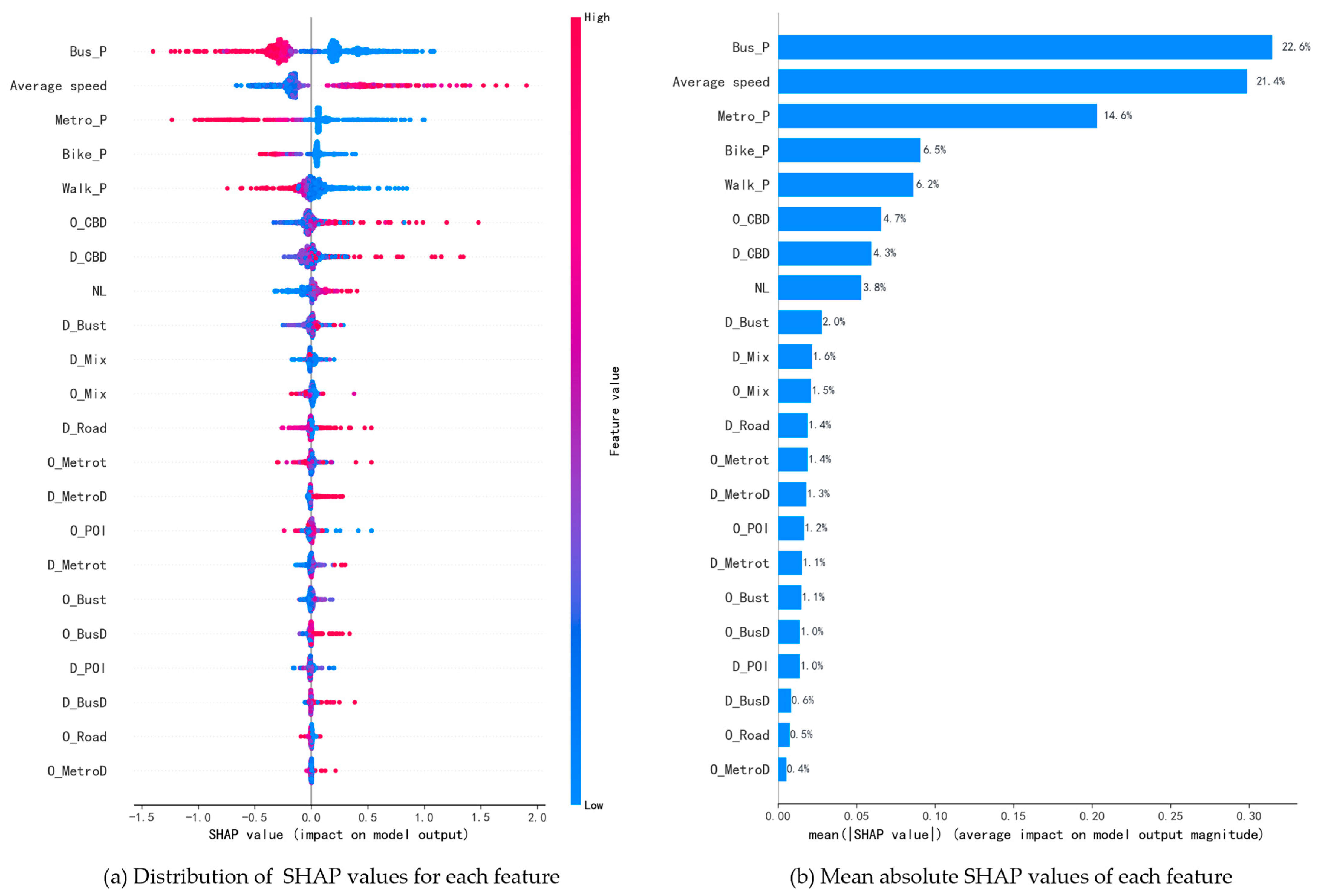
• All explanatory variables collectively contributed to the prediction of CO₂ emissions, with transportation-related variables accounting for 75.1% of the model’s explanatory power and built environment factors contributing the remaining 24.9%.
• The analysis indicates that bus usage, average speed, and metro usage are the top three contributors to carbon emissions, followed by cycling, walking, destination distance to the CBD, and non-linear travel route.
• The PDP analysis reveals that substantial emission reductions are observed only when the modal shares of bus, metro, and cycling exceed approximately 40%, 40%, and 30%, respectively. This indicates the existence of threshold effects, where merely modest increases in sustainable mode shares may not yield significant carbon benefits unless these thresholds are surpassed.
• In addition, travel-related carbon emissions are generally lower when the spatial distance between trip origins and destinations falls within the range of 10 to 11 km from the central business district (CBD). This suggests that mid-range trips at this distance are associated with greater use of public transit and non-motorized modes, thereby contributing to more efficient and carbon-efficient travel. These findings are consistent with global research—for instance, Ewing and Cervero [26] found that mid-range commutes in U.S. cities are more likely to involve active transportation, while Akuh et al. [10,11,12] demonstrated that balanced land use in European new towns reduces reliance on high-emission travel modes. Together, these parallels suggest the broader applicability of our analytical framework for sustainable urban transport planning.

These findings offer several practical policy implications for advancing sustainable urban mobility. Based on our findings, policymakers could foster the balanced integration of low-carbon transportation modes, such as buses, metro, and cycling, while optimizing urban form and connectivity to achieve substantial emission reductions, contributing to sustainable urban mobility. Firstly, the observed threshold effects suggest that incremental increases in public and active mode shares may be insufficient for achieving meaningful emission reductions. Instead, urban transport policies should aim to exceed modal share thresholds—approximately 40% for both bus and metro, and 30% for cycling—through targeted investment, service improvements, and user incentives. This could include expanding dedicated cycling infrastructure, increasing the frequency and reliability of metro and bus services, and introducing demand-side incentives such as fare subsidies or congestion pricing for car use. Secondly, the finding that carbon emissions are minimized for trips occurring within a 10–11 km radius of the central business district underscores the significance of polycentric urban development. Encouraging mid-range, transit-oriented development (TOD) can promote efficient public transit usage while discouraging both short car trips and excessively long commutes. Urban planning strategies that optimize the spatial allocation of residential and employment functions within this range—particularly along major transit corridors—can further strengthen the potential for emission mitigation through multimodal travel. Moreover, since carbon emissions increase with higher average travel speeds and route non-linearity, traffic management strategies should prioritize efficient but moderate-speed operations and minimize detours through better route planning and signal coordination. Finally, real-time carbon feedback systems could be embedded in smart mobility apps to encourage travelers to select lower-emission travel options and help municipal authorities refine emission control strategies.

7. Limitations and Future Directions

This study has several limitations that should be addressed in future research. Firstly, the dataset is based on 60 individuals in Beijing from 2007 to 2012, primarily aged 22–30, which may limit the generalizability of the findings. While the relationships identified between travel modes, spatial attributes, and carbon emissions are structurally robust, their transferability to other cities, age groups, or countries may be influenced by differences in transportation infrastructure, cultural norms, and policy contexts. In addition, while the carbon emission modeling framework demonstrates strong explanatory power, it is subject to uncertainties inherent in GPS-based trajectory data and derived features such as distance and speed. Although a full sensitivity analysis is beyond the scope of this study, robustness checks were performed to address potential sources of error. Specifically, we applied strict data filters to mitigate GPS drift and removed segments with inconsistent speed or mode labels. We also tested the sensitivity of CO₂ estimates to small variations in input features, finding that emissions varied by less than ±7%. These checks suggest that the results are stable and the framework is reliable for identifying structural emission patterns in multimodal travel. Therefore, future research should incorporate formal sensitivity or uncertainty analyses and utilize more recent, large-scale multimodal datasets to enhance the robustness and generalizability of the findings.

References

1. Chen, S.; Long, H.; Chen, B.; Feng, K.; Hubacek, K. Urban Carbon Footprints across Scale: Important Considerations for Choosing System Boundaries. Appl. Energy 2020, 259, 114201. [Google Scholar] [CrossRef]
2. Zhang, Z.; Yu, X.; Hou, Y.; Chen, T.; Lu, Y.; Sun, H. Carbon Emission Patterns and Carbon Balance Zoning in Urban Territorial Spaces Based on Multisource Data: A Case Study of Suzhou City, China. IJGI 2023, 12, 385. [Google Scholar] [CrossRef]
3. Zhu, Z.; Lu, C. Life Cycle Assessment of Shared Electric Bicycle on Greenhouse Gas Emissions in China. Sci. Total Environ. 2023, 860, 160546. [Google Scholar] [CrossRef]
4. Zou, Y.; Xiao, G.; Li, Q.; Biancardo, S.A. Intelligent Maritime Shipping: A Bibliometric Analysis of Internet Technologies and Automated Port Infrastructure Applications. J. Mar. Sci. Eng. 2025, 13, 979. [Google Scholar] [CrossRef]
5. Li, W.; Bao, L.; Li, Y.; Si, H.; Li, Y. Assessing the Transition to Low-Carbon Urban Transport: A Global Comparison. Resour. Conserv. Recycl. 2022, 180, 106179. [Google Scholar] [CrossRef]
6. Li, W.; Bao, L.; Wang, L.; Li, Y.; Mai, X. Comparative Evaluation of Global Low-Carbon Urban Transport. Technol. Forecast. Soc. Change 2019, 143, 14–26. [Google Scholar] [CrossRef]
7. Li, J.; Jiang, C.; Han, K.; Yu, Q.; Zhang, H. High-Resolution Spatiotemporal Inference of Urban Road Traffic Emissions Using Taxi GPS and Multi-Source Urban Features Data: A Case Study in Chengdu, China. Urban Inform. 2024, 3, 17. [Google Scholar] [CrossRef]
8. Li, W.; Pu, Z.; Li, Y.; Tu, M. How Does Ridesplitting Reduce Emissions from Ridesourcing? A Spatiotemporal Analysis in Chengdu, China. Transp. Res. Part D Transp. Environ. 2021, 95, 102885. [Google Scholar] [CrossRef]
9. Ren, L.; Guo, X.; Wu, J.; Singh, A.K. Data Mining and Spatio-Temporal Characteristics of Urban Road Traffic Emissions: A Case Study in Shijiazhuang, China. PLoS ONE 2023, 18, e0295664. [Google Scholar] [CrossRef] [PubMed]
10. Herbruggen, B.V.; Logghe, S. Tremove version 2.3 simulation model for european environmental transport policy analysis. In Proceedings of the 14th International Symposium “Transport and Air Pollution”, Graz, Germany, 1–3 June 2005. [Google Scholar]
11. Schade, B.; Wiesenthal, T. Developments in Energy Use for Transport in 27 European Union Countries through 2030: Outcome of iTREN-2030 Project. Transp. Res. Rec. 2011, 2252, 31–39. [Google Scholar] [CrossRef]
12. Akuh, R.; Zhong, M.; Raza, A.; Dong, Y. A Method for Evaluating the Balance of Land Use and Multimodal Transport System of New Towns/Cities Using an Integrated Modeling Framework. Multimodal Transp. 2023, 2, 100063. [Google Scholar] [CrossRef]
13. Cheng, B.; Li, J.; Su, H.; Lu, K.; Chen, H.; Huang, J. Life Cycle Assessment of Greenhouse Gas Emission Reduction through Bike-Sharing for Sustainable Cities. Sustain. Energy Technol. Assess. 2022, 53, 102789. [Google Scholar] [CrossRef]
14. Zhao, J.; Yuan, C.; Mao, X.; Ma, N.; Duan, Y.; Zhu, J.; Wang, H.; Tian, B. Identifying the Nonlinear Impacts of Road Network Topology and Built Environment on the Potential Greenhouse Gas Emission Reduction of Dockless Bike-Sharing Trips: A Case Study of Shenzhen, China. IJGI 2024, 13, 287. [Google Scholar] [CrossRef]
15. Shi, W.; Xiang, Y.; Ying, Y.; Jiao, Y.; Zhao, R.; Qiu, W. Predicting Neighborhood-Level Residential Carbon Emissions from Street View Images Using Computer Vision and Machine Learning. Remote Sens. 2024, 16, 1312. [Google Scholar] [CrossRef]
16. Liu, J.; Han, K.; Chen, X.; Ong, G.P. Spatial-Temporal Inference of Urban Traffic Emissions Based on Taxi Trajectories and Multi-Source Urban Data. Transp. Res. Part C Emerg. Technol. 2019, 106, 145–165. [Google Scholar] [CrossRef]
17. Handy, S.; Cao, X.; Mokhtarian, P.L. Self-Selection in the Relationship between the Built Environment and Walking: Empirical Evidence from Northern California. J. Am. Plan. Assoc. 2006, 72, 55–74. [Google Scholar] [CrossRef]
18. Yu, W.; Xia, L.; Cao, Q. A Machine Learning Algorithm to Explore the Drivers of Carbon Emissions in Chinese Cities. Sci. Rep. 2024, 14, 23609. [Google Scholar] [CrossRef]
19. Zeng, J.; Liu, Y.; Ding, J.; Yuan, J.; Li, Y. Estimating On-Road Transportation Carbon Emissions from Open Data of Road Network and Origin-Destination Flow Data V1. arXiv 2024, arXiv:2402.05153. [Google Scholar] [CrossRef]
20. Pu, Y.; Yang, C.; Liu, H.; Chen, Z.; Chen, A. Impact of License Plate Restriction Policy on Emission Reduction in Hangzhou Using a Bottom-up Approach. Transp. Res. Part D Transp. Environ. 2015, 34, 281–292. [Google Scholar] [CrossRef]
21. Ibarra-Espinosa, S.; Ynoue, R.; O’Sullivan, S.; Pebesma, E.; Andrade, M.d.F.; Osses, M. VEIN v0.2.2: An R Package for Bottom–up Vehicular Emissions Inventories. Geosci. Model Dev. 2018, 11, 2209–2229. [Google Scholar] [CrossRef]
22. Sun, D.; Zhang, K.; Shen, S. Analyzing Spatiotemporal Traffic Line Source Emissions Based on Massive Didi Online Car-Hailing Service Data. Transp. Res. Part D Transp. Environ. 2018, 62, 699–714. [Google Scholar] [CrossRef]
23. Luo, X.; Dong, L.; Dou, Y.; Zhang, N.; Ren, J.; Li, Y.; Sun, L.; Yao, S. Analysis on Spatial-Temporal Features of Taxis’ Emissions from Big Data Informed Travel Patterns: A Case of Shanghai, China. J. Clean. Prod. 2017, 142, 926–935. [Google Scholar] [CrossRef]
24. Li, W.; Wang, L.; Pu, Z.; Cheng, L.; Yang, L. What Determines the Real-World CO2 Emission Reductions of Ridesplitting Trips? Travel Behav. Soc. 2024, 35, 100734. [Google Scholar] [CrossRef]
25. Ntziachristos, L.; Samaras, Z. Methodology for the calculation of exhaust emissions. In EMEP/EEA Emission Inventory Guidebook; SNAPs 070100-070500, NFRs 1A3bi-iv; European Environment Agency: Copenhagen, Denmark, 2024. [Google Scholar]
26. Ewing, R.; Cervero, R. Travel and the Built Environment. J. Am. Plan. Assoc. 2010, 76, 265–294. [Google Scholar] [CrossRef]
27. Friedman, J.H. Greedy Function Approximation: A Gradient Boosting Machine. Ann. Statist. 2001, 29, 1189–1232. [Google Scholar] [CrossRef]
28. Prokhorenkova, L.; Gusev, G.; Vorobev, A.; Dorogush, A.V.; Gulin, A. CatBoost: Unbiased Boosting with Categorical Features V5. arXiv 2017, arXiv:1706.09516. [Google Scholar] [CrossRef]
29. Ke, G.; Meng, Q.; Finley, T.; Wang, T.; Chen, W.; Ma, W.; Ye, Q.; Liu, T.-Y. LightGBM: A Highly Efficient Gradient Boosting Decision Tree. In Proceedings of the 31st International Conference on Neural Information Processing Systems, Long Beach, CA, USA, 4–9 December 2017; pp. 3149–3157. [Google Scholar]
30. Chen, T.; Guestrin, C. XGBoost: A Scalable Tree Boosting System. In Proceedings of the Proceedings of the 22nd ACM SIGKDD International Conference on Knowledge Discovery and Data Mining, San Francisco, CA, USA, 13–17 August 2016; Association for Computing Machinery: New York, NY, USA; pp. 785–794. [Google Scholar]
31. Lundberg, S.M.; Erion, G.G.; Lee, S.-I. Consistent Individualized Feature Attribution for Tree Ensembles V3. arXiv 2018, arXiv:1802.03888. [Google Scholar] [CrossRef]
Figure 1. Participant demographics. (Source: Own elaboration based on the GeoLife dataset.)
Sustainability 17 06983 g001
Figure 2. Multimodal travel description diagram.
Sustainability 17 06983 g002
Figure 3. SHAP-based feature importance and bee swarm plot. (Source: Own calculation based on the well-trained XGBoost model).
Sustainability 17 06983 g003
Figure 4. PDPs for determinants of multimodal travel. (Source: Own calculation based on the well-trained XGBoost model).
Sustainability 17 06983 g004