Beyond the Detour: Modeling Traffic System Shocks After the Francis Scott Key Bridge Failure

Abstract

This research examines the traffic disruptions resulting from the collapse of the Francis Scott Key Bridge in Baltimore, utilizing advanced econometric methods and real-time ClearGuide data. Employing Fixed Effects (FEs), Mixed Effects (MEs), Difference-in-Differences (DiDs), and stratified regression models, the study uniquely examines the impacts of congestion across Immediate, Fall, and Winter periods, distinctly separating AM and PM peak patterns. Significant findings include severe PM peak congestion, up to four times greater than AM peak congestion, particularly on critical corridors such as the Harbor Tunnel Thruway northbound and MD-295 northbound. Initial route-level impacts were heterogeneous, gradually becoming uniform as the network adapted. The causal DiD analysis provides strong evidence that increased congestion is causally linked to proximity to the collapse. It is anticipated that incorporating the suggested framework will yield insightful information for stakeholders and decision-makers, such as targeted freight restriction, peak-hour dynamic pricing, corridor-specific signal adjustments, and investments in real-time traffic monitoring systems to strengthen transportation network resilience.

1. Introduction

Urban transportation networks typically function based on well-established daily and weekly rhythms, with traffic volumes displaying foreseeable patterns during peak and off-peak hours on workdays, a well-documented phenomenon in traffic engineering research. While these predictable fluctuations from events like holidays or planned roadwork pose management challenges, they remain within a recognized scope of possibilities [1]. A fundamentally different and more severe problem emerges from abrupt, catastrophic infrastructure failures. Occurrences like the collapse of a critical bridge unexpectedly sever major transportation arteries without warning, activating system-wide shockwaves that extend far beyond the immediate incident site.

A fundamentally diverse and more severe problem emerges from abrupt, catastrophic infrastructure failures. Occurrences like the collapse of a critical bridge unexpectedly sever major transportation arteries without warning, activating system-wide shockwaves that extend far beyond the immediate incident site [2,3]. Long-standing commuting routines are disrupted as motorists seek alternative routes, straining secondary roads that are ill-prepared for spikes in cross-town traffic. Even seemingly minor disruptions to a key thoroughfare or transit line can cascade through the larger network, underscoring the importance of maintaining redundancies to absorb disruptions gracefully [4]. These events often result in system-wide performance degradation that extends well beyond the immediate vicinity of the incident [3].

Timely and effective responses to these traffic disruptions depend on the availability and efficient use of accurate real-time data. While previous studies have utilized robust econometric methodologies to evaluate traffic disruptions, including Fixed Effects (FEs), Mixed Effects (MEs), and Difference-in-Difference (DiD) [5,6,7,8], they often face two critical limitations that leave a gap in our understanding. First, most studies rely on a single modeling approach, which may not fully capture the multifaceted nature of system-wide impacts. An analysis might reveal an average network effect (FE), group-level variations (ME), or a causal impact (DiD), but rarely are these perspectives integrated to form a holistic picture. Crucially, few studies have systematically compared the insights derived from these different models within a singular, catastrophic event context, leaving a critical research gap in understanding which methodologies offer the most robust and actionable insights for crisis management. Second, many analyses have traditionally relied on static or retrospective data, limiting their ability to inform rapid and adaptive responses. The recent collapse of the Francis Scott Key Bridge in Baltimore, Maryland, on 26 March 2024, provides an urgent and unparalleled opportunity to address these gaps. This catastrophic event, which served as a primary artery carrying over 34,000 vehicles daily, offers a real-world laboratory for in-depth analysis [9,10]. This study leverages a high-frequency dataset from ClearGuide, a real-time traffic analytics platform, to overcome the limitations of past research. The primary contribution of this paper is the development and implementation of a multi-pronged comparative framework to rigorously quantify and interpret the traffic impacts of the bridge collapse. Specifically, this research aims to

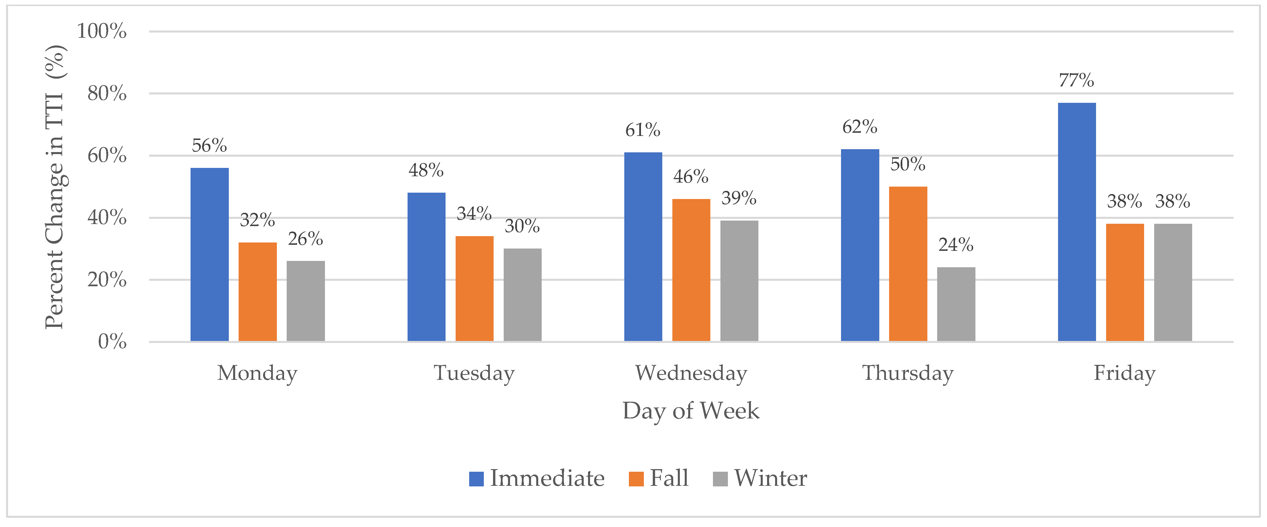
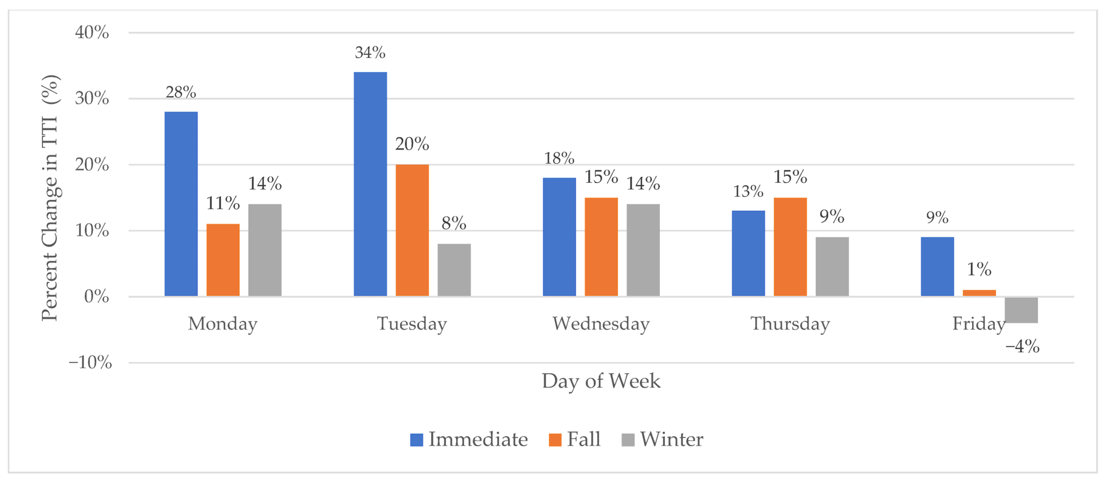
• Assess system-wide traffic disruptions with Travel Time Index (TTI) caused by the bridge collapse across distinct temporal dimensions, including the Immediate, Fall, and Winter periods, with a clear delineation between AM and PM peak hours.
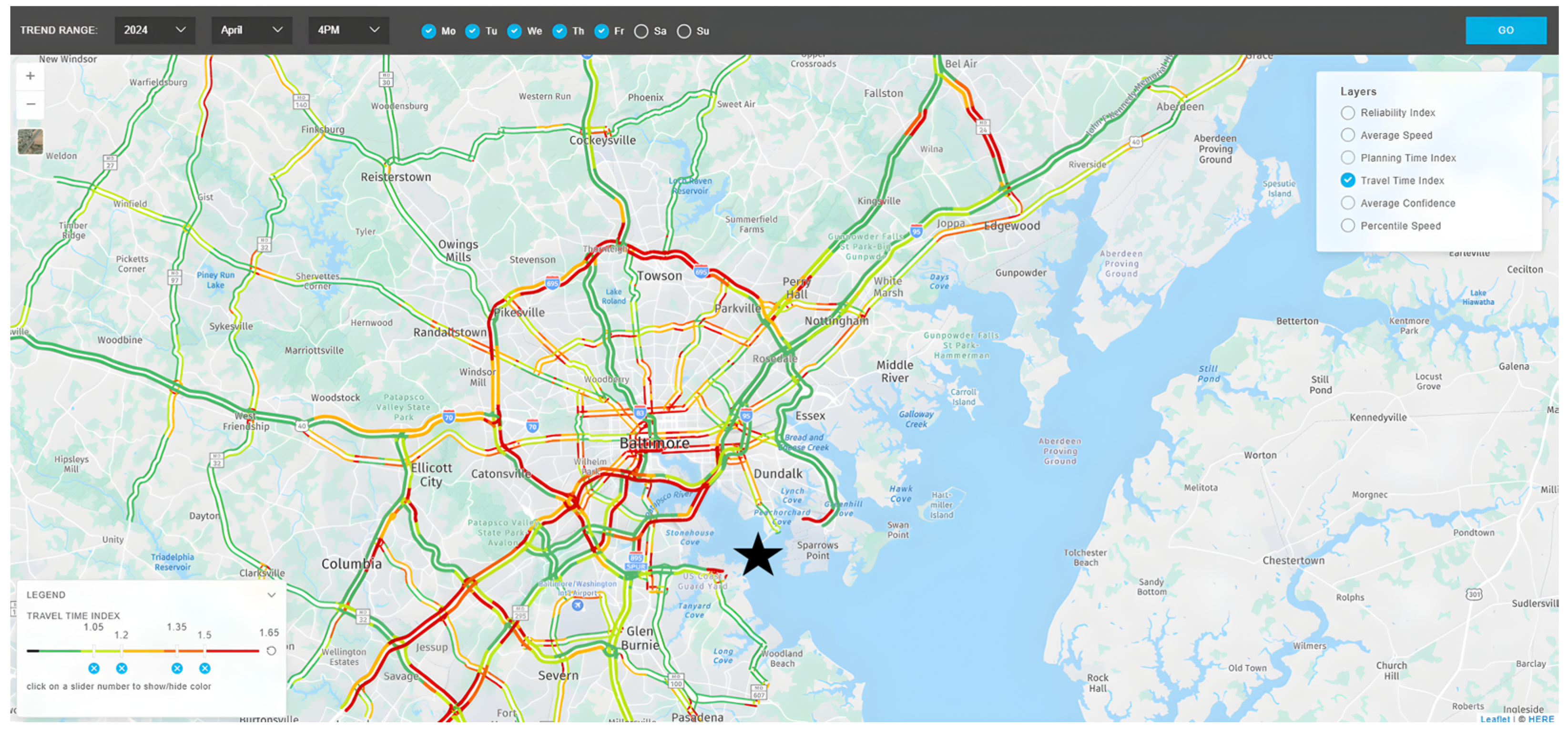
• Identify and visualize corridors exhibiting the most significant performance degradation following the bridge collapse.
• To develop and implement a multi-pronged framework that incorporates Fixed Effects, Mixed Effects, Difference-in-Differences (DiDs), and stratified regression models to quantify the impacts attributable to the bridge collapse.

By achieving these objectives, this study makes several key contributions:

• Methodologically, it develops and applies a comparative analytical framework that systematically contrasts the performance and insights of multiple advanced econometric models on a singular catastrophic event. This approach offers valuable guidance to researchers and practitioners on model selection for future disaster-impact analyses.
• Empirically, this research provides the first comprehensive, multi-dimensional quantification of the traffic impacts resulting from the Francis Scott Key Bridge collapse, creating a crucial benchmark for one of the most significant transportation disruptions in recent U.S. history.
• Practically, the findings offer targeted, actionable insights for transportation agencies to develop more resilient networks and effective real-time traffic management strategies, moving beyond system-wide averages to address critical, localized “hotspots.”

The remainder of this paper is organized as follows: Literature review synthesizes existing findings, discusses methodological approaches, and highlights gaps that inform the objectives and design of the present study. Method and Data explain modeling frameworks and describe data sources used for the analysis. Results and Discussion present the empirical findings from each model and compare the insights and interpret the results, highlighting implications, and the Conclusion summarizes the key findings and recommendations for future work.

2. Literature Review

2.1. Real-Time Traffic Management and Intelligent Transportation Systems

Modern traffic management integrates many data streams. These include sensors, GPS probes, connected-car networks, and smartphone applications. This integration helps us understand sewer and water currents and see what lies ahead for roads [11]. Monitoring traffic in real time allows us to track congestion and keep traffic flowing. Yet, this is very challenging. Roads experience sudden, severe incidents. Could a proactive approach succeed? Such a shift would represent a significant advancement for transportation systems [12,13,14].

2.2. Precedents in Disruption Analysis: Case Studies and Methodologies

A significant amount of literature has documented the cascading effects of major infrastructure failures, providing a foundation for understanding both system impacts and effective analytical techniques [15,16]. Case studies of catastrophic events, such as the 2007 collapse of the I-35W Bridge in Minneapolis, which forced about 140,000 daily vehicles onto new routes [17], and the sudden failure of the West Seattle Bridge, which led to freight rerouting and logistical issues [18], vividly illustrate these severe consequences.

After the initial shock, research consistently finds that affected systems adapt to a new, albeit often less efficient, equilibrium [19]. This understanding has propelled increased research into network resilience, with studies showing that network redundancy significantly aids recovery [20,21]. Furthermore, it has become evident that the economic impacts of such failures can spread broadly across complex supply chains [22,23].

To accurately measure these multifaceted and complex impacts, researchers employ various econometric tools [24]. Fixed Effect (FE) panel models, for instance, are crucial for isolating specific effects by effectively controlling for time-invariant roadway characteristics [25]. For data exhibiting hierarchical structures, Mixed-Effect Models (ME) and generalized linear mixed models (GLMM) prove highly effective, especially when analyzing factors where group-level variance is significant, such that traffic systems or regional economic analyses [26,27] often arise. Moreover, to establish robust causal inferences and account for underlying time trends that could otherwise bias results, the Difference-in-Differences (DiDs) approach is frequently utilized in transportation studies [28,29].

2.3. Emerging Approaches and Remaining Gaps

Recent advancements in machine learning have introduced powerful new tools for network analysis. Notably, Graph Neural Networks (GNNs) have emerged as a state-of-the-art approach for modeling complex transportation systems. One study demonstrated the use of GNNs as computationally efficient surrogate models for assessing the seismic reliability of highway bridge systems, capable of capturing complex network topologies and providing rapid, system-level performance evaluations [30]. Other research has leveraged heterogeneous GNNs to solve the traffic assignment problem, predicting traffic flow patterns with high accuracy by learning spatial dependencies across the network [31]. These data-driven methods excel at prediction and large-scale simulation.

However, a key challenge with some advanced machine learning models, including GNNs, can be their limited interpretability in failure-critical scenarios. While they can predict what will happen with high accuracy, it can be more difficult to extract clear, policy-relevant parameters that explain why it is happening (e.g., the specific marginal effect of a freight restriction policy). This highlights a distinction between models optimized for prediction and those designed for causal explanation and policy parameterization.

2.4. Research Gaps and Contributions

Existing research, therefore, presents a strong foundation but also a distinct research gap. While traditional econometric models like FE, ME, and DiD offer high interpretability, they are rarely applied in a comparative framework to a single event. Conversely, while emerging GNN-based methods offer powerful predictive capabilities, they may not provide the same level of granular, interpretable insights needed for direct policy evaluation. This study fills that gap by developing a multi-faceted framework that systematically applies and compares four distinct econometric models. By doing so, we move beyond a single analytical viewpoint to provide a holistic and detailed assessment of a major network shock, revealing nuanced patterns of disruption, adaptation, and persistent local stress that might be missed by any single method alone. This comparative approach is designed not to replace predictive models, but to complement them by providing a deep, explanatory understanding of the system’s response to crisis.

3. Methods and Data

3.1. Study Design and Data Sources

The core performance measure used to quantify traffic congestion is the Travel Time Index (TTI), a standardized metric defined as the ratio of peak period travel time to free-flow travel time [32,33]. A TTI of 1.3, for instance, means a trip takes 30% longer than under ideal, free-flow conditions [34]. We selected TTI as our primary dependent variable not only for its intuitive nature but also because it is a key performance indicator endorsed by the Federal Highway Administration (FHWA) for its robust comparative capabilities in monitoring mobility and reliability [32,35].

This analysis is made possible by high-resolution traffic data sourced from Iteris ClearGuide, a widely used transportation analytics platform (Figure 1). It aggregates and processes anonymized GPS probe data from a massive fleet of connected vehicles and mobile devices to produce reliable travel time and speed metrics at fine spatial and temporal scales. The “star” in the map indicated the collapse of the Francis Scott Key Bridge.

3.2. Data Structure and Processing

Our dataset spans from September 2023 to February 2025, allowing for a robust before-and-after analysis across different seasons. To capture both the immediate shock and longer-term shifts in traffic patterns, we structured the analysis into three distinct periods:

• Immediate: 26 March–25 April 2024 (Post-Collapse) vs. 26 February–25 March 2024 (Baseline).
• Fall: September–November 2024 (Post-Collapse) vs. September–November 2023 (Baseline).
• Winter: December 2024–February 2025 (Post-Collapse) vs. December 2023–February 2024 (Baseline).

The study focuses on 30 major corridors in the Baltimore region; each selected for its critical role in the regional transportation network surrounding the site of the Francis Scott Key Bridge collapse. These corridors serve as essential components for local and through traffic, particularly in the context of the I-695 Baltimore Beltway, which previously relied on the Key Bridge for seamless southeastern flow of vehicles, including those carrying hazardous materials not permitted in Baltimore’s tunnels.

For the Difference-in-Differences analysis, corridors were classified based on their centroid distance from the collapsed bridge. Routes within a 10-mile radius were designated as ‘Proximate’ (Treated), while those beyond 10 miles were categorized as ‘Distant’ (Control). This distinction aimed to capture the immediate impact zone relative to the severed artery and the location of the primary alternative crossings: the I-95 Fort McHenry Tunnel and I-895 Harbor Tunnel. Both tunnels, while serving significant regional and interstate traffic under the Patapsco River, restrict hazardous material transport, further underscoring the indispensable function formerly provided by the Key Bridge.

All datasets underwent a rigorous cleaning and validation process using Python 3.11 scripts. This included the elimination of null records, the smoothing of extreme outliers (defined as values outside ±2.5 standard deviations from a rolling median), and the harmonization of all timestamps. Analyses were restricted to weekday morning (7:00–9:00) and evening (16:00–18:00) peak periods to maintain consistency with standard traffic analysis protocols [36].

We acknowledge that classifying corridors into ‘Proximate’ and ‘Distant’ groups based on Euclidean distance is a simplification that does not capture the full complexity of network topology or potential socioeconomic confounders. However, for an analysis focused on the immediate shock from a catastrophic infrastructure failure, this classification is conceptually robust. The initial rerouting decisions by thousands of drivers are overwhelmingly dictated by physical proximity to the severed artery and the location of the primary alternative crossings (the two tunnels). Therefore, Euclidean distance serves as a strong and intuitive first-order proxy for identifying the group of corridors most directly and immediately impacted by the event. This approach prioritizes the initial physical shockwave over longer-term, behaviorally adapted route choices, which could be explored in future work using more granular network-based distance metrics.

3.3. Multi-Faceted Analytical Framework

With the data prepared, we applied four distinct but complementary statistical models to the data for each of the three analysis periods. Each model is designed to answer a slightly different question, together providing a holistic understanding of the event.

3.3.1. Fixed Effects (FE) Model: Quantifying Average Change

First, to assess the average impact of the collapse on traffic, we used a Fixed Effect (FE) panel model. By controlling characteristics unique to each corridor (e.g., geometry, lanes, baseline culture), the FE model isolates the average change in TTI on each route after the collapse [37,38]. As specified in Equation (1), this model provides a robust baseline estimate of overall network disruption [37].

$${TTI}_{it}={\beta }_0+{\beta }_1{Post}_t+{{\beta }_2{Peak}_t+{\beta }_3\left({Post}_t\times {Peak}_{it}\right)+\alpha }_i+{\gamma }_t+{\epsilon }_{it}$$

(1)

where ${TTI}_{it}$ is the Travel Time Index for corridor i at time t; ${Post}_t$ is a dummy variable equal to 1 for the post-collapse period and 0 otherwise; ${Peak}_{it}$ is a dummy variable equal to 1 for the PM peak (16:00–18:00) and 0 for the AM peak (7:00–9:00); the interaction term captures the differential effect in the PM peak after the collapse; ${\alpha }_i$ represents time-invariant corridor-specific fixed effects (e.g., geometry, number of lanes); ${\gamma }_t$ represents time-period-specific fixed effects (e.g., day-of-week); and ${\epsilon }_{it}$ is the error term.

3.3.2. Mixed Effect (ME) Model: Exploring Group-Level Variation

To assess differences between spatial groups, we used a Mixed Effect Model (ME). Unlike the FE model, the ME captures variance between ‘Proximate’ and ‘Distant’ groups while accounting for repeated observations within routes [39,40]. As shown in Equation (2), this model includes a random intercept for each route, allowing a more nuanced view of how proximity mediates traffic impacts [41].

$${TTI}_{it}={\beta }_0+{\beta }_1{Post}_t+{\beta }_2{Proximity}_i+u_i+{\epsilon }_{it}$$

(2)

where ${TTI}_{it}$ is the Travel Time Index for corridor i at time t; Postt is a dummy variable for the post-collapse period; ${Proximity}_i$ is a time-invariant dummy variable equal to 1 if a corridor is in the ‘Proximate’ group (within 10 miles of the collapse) and 0 if it is in the ‘Distant’ group; $u_i$ is the random intercept for each corridor, capturing unobserved corridor-specific heterogeneity; and ${\epsilon }_{it}$ is the error term.

3.3.3. Difference-in-Differences (DiD) Model: Isolating the Causal Impact

To rigorously measure the causal effect of the bridge collapse, we used a Difference-in-Difference (DiD) model [42,43]. This approach compares TTI changes in the ‘Proximate’ group to the ‘Distant’ control group. The DiD estimator (the interaction term in Equation (3)) captures the additional impact on treated routes, netting out any regional trends during the post-collapse period [37]. A critical assumption for the DiD model is that the treatment and control groups would have followed parallel trends in the absence of the treatment. To validate this assumption, we examined traffic patterns in the four weeks preceding the collapse. As shown in Figure 2, the average TTI for both the proximate (treatment) and distant (control) groups followed parallel trajectories during the pre-collapse period for both AM and PM peaks, indicating the absence of pre-existing differential trends [44]. This provides strong support for the use of the DiD model to isolate the causal impact of the collapse.

$${TTI}_{it}={\beta }_0+{\beta }_1{Post}_t+{\beta }_2{Treatment}_i+{\beta }_3\left({{Post}_t\times Treatment}_i\right)+{\alpha }_i+{\gamma }_t+{\epsilon }_{it}$$

(3)

where ${TTI}_{it}$ is the Travel Time Index for corridor i at time t; Postt is the dummy for the post-collapse period; ${Treatment}_i$ is the dummy variable equal to 1 for corridors in the ‘Proximate’ group (the treatment group) and 0 for the ‘Distant’ group (the control group); the interaction term (${{Post}_t\times Treatment}_i$) is the DiD estimator, capturing the causal effect of the collapse on the treatment group; ${\alpha }_i$ represents corridor-specific fixed effects; ${\gamma }_t$ represents time-period-specific fixed effects; and ${\epsilon }_{it}$ is the error term.

Figure 2 visually validates the parallel trends assumption, a critical prerequisite for the Difference-in-Differences (DiD) analysis presented in this study. It plots the average Travel Time Index (TTI) for both the proximate (treatment) and distant (control) corridors in the four weeks immediately preceding the bridge collapse. The nearly identical trajectories for both AM and PM peak periods provide strong visual support that the two groups shared a common trend before the event, thereby strengthening the causal interpretation of the DiD model’s findings.

3.3.4. Stratified Modeling of High-Impact Routes: Focus on High-Impact Corridors

Recognizing that network averages can mask extreme congestion, we performed a stratified analysis. We identified the top 20% of affected corridors and re-ran our FE and ME models on this high-impact subset [45]. This revealed how general network effects differ from acute conditions on the most burdened routes [37]. The approach provides granular insights for targeted planning and investment [46].

3.4. A Framework for Synthesized Analysis

These four analytical approaches—Fixed Effects, Mixed-Effects, Difference-in-Differences, and Stratified Analysis—form a comprehensive framework. Each model offers a unique perspective: FE covers average change, ME explores spatial groups, DiD measures causal impact, and stratified analysis shows high-impact dynamics.

Figure 3 is a graphical representation of our analysis strategy, which takes us from digits and numbers to ideas. The visual depiction illustrates how the four modeling methods interrelate with each other, providing an exhaustive foundation from which to draw any conclusion. The biggest advantage of this approach is that it utilizes triangulation, in which results are cross-checked using four different but equally valid analytical methods. These tactics have two major benefits: they enhance the reliability of findings and make it possible to uncover insights that might have been overlooked through a single type of analysis. That is what distinguishes a truly comprehensive impact assessment from a more limited analysis.

4. Results and Discussion

This section presents the empirical findings of the study, beginning with a descriptive overview of the traffic impacts, followed by a multi-faceted modeling analysis to quantify the effects and attribute causality.

4.1. The Profile of a Network Under Stress: Descriptive and Temporal Patterns

In the period immediately after the bridge collapse, the statistics proved quite dramatically how a tentacled network lay under stress. The evening rush-hour commuter bore the brunt of it. Averaged over all periods, PM peak hours (16:00–18:00) had both higher mean Travel Time Index (TTI) values and greater volatility than AM peak hours [47]. For example, the average PM peak TTI reached 2.26 in the immediate period following the collapse. This figure means trips took 126% longer than in free-flow conditions. The PM peak impact was far more severe than the AM peak TTI of 1.45. The intense pressure during the PM peak, especially heading south, likely reflected the combined effects of commuter and freight traffic on limited alternative roads [48].

A closer look at the daily movements (Figure 4 and Figure 5) reveals how the disruption intersected with weekly travel rhythms. The initial shock was most acute at the end of the week; in the immediate post-collapse period, the Friday PM peak saw a dramatic 77% increase in TTI, suggesting that the typical higher-volume end-of-week traffic severely exacerbated the initial chaos. However, this pattern evolved over time. In the subsequent Fall and Winter periods, the most significant congestion shifted to mid-week, with Wednesday PM peaks consistently showing a greater TTI increase than Fridays. This temporal shift may indicate a complex adaptation process, potentially involving changes in remote work patterns, altered commercial delivery schedules, or other behavioral adjustments as commuters and logistics operators settled into a new, albeit less efficient, weekly routine [49,50].

4.2. The Spatiotemporal Evolution of Congestion

The traffic maps in Figure 6 trace the transition from the initial widespread shock to persistent bottlenecks across the network.

By the peak of PM after the event (Figure 6a), severe congestion emerged, with key arteries such as the Harbor Tunnel Thruway (NB) and MD-295 (NB) experiencing deep saturation (TTI > 2.0). The AM peak (Figure 6b) shifted congestion to localized detour routes, such as Interstate 95 (southbound). These patterns solidified by Fall (Figure 6c), showing recurring congestion and habitual detour use. In Winter, while the network stabilized, persistent delays remained near tunnel access points (Figure 6e,f), forming lasting congestion “hotspots”.

4.3. Multi-Faceted Modeling Analysis

To quantify the impact of the collapse, we employed a four-part modeling framework. Each model offers a distinct perspective, contributing to a comprehensive assessment.

4.3.1. Quantifying the Average Impact and Network Adaptation (Fixed Effect and Mixed Effect Models)

The Fixed Effect (FE) models, controlling for each route’s unique traits, confirm the main findings statistically (

Table 1. Fixed effect regression results for AM and PM peak TTI changes by period.

Period	Term	Estimate	Std. Error	p-Value	Confidence Interval (Lower)	Confidence Interval (Upper)
Immediate	Intercept	1.428	0.473	0.003	0.4989	2.3563
	Period (Before)	−0.223	0.001	<0.001	−0.2249	−0.2202
	Peak (PM)	0.825	0.001	<0.001	0.8227	0.8273
	Interaction (Before × PM)	−0.624	0.002	<0.001	−0.6269	−0.6203
	Adjusted Within R-squared	0.189
	AIC	18,354,326.50
	F-Statistics	306,506.69		<0.001
Fall	Intercept	1.390	0.002	<0.001	1.3864	1.3942
	Period (Before)	−0.157	0.003	<0.001	−0.1625	−0.1514
	Peak (PM)	0.729	0.003	<0.001	0.7232	0.7343
	Interaction (Before × PM)	−0.455	0.004	<0.001	−0.4626	−0.4469
	Adjusted Within R-squared	0.175
	AIC	44,862,201.07
	F-Statistics	814,159.64		<0.001
Winter	Intercept	1.294	0.002	<0.001	1.2902	1.2972
	Period (Before)	−0.095	0.003	<0.001	−0.0999	−0.0900
	Peak (PM)	0.502	0.003	<0.001	0.4966	0.5065
	Interaction (Before × PM)	−0.331	0.004	<0.001	−0.3381	−0.3240
	Adjusted Within R-squared	0.155
	AIC	41,169,378.77
	F-Statistics	464,494.59		<0.001

). Following the collapse, TTI in the PM peak increased by 0.847 units—nearly four times the AM peak increase of 0.223 (p < 0.001 for both). Over time, both effects shrank but stayed significant, with the PM impact consistently 2–4 times larger [51]. This supports prior research on evening commute vulnerability [48].

The Mixed Effect (ME) models corroborate these findings while adding a crucial insight into spatial heterogeneity (

Table 2. Mixed effect regression results for AM and PM peak TTI changes by period.

Period	Term	Estimate	Std. Error	p-Value	Conditional R2	AIC
Immediate	Intercept	1.449	0.098	<0.001	0.5454	17,444,867.424
	Period (Before)	−0.257	0.005	<0.001
	Peak (PM)	0.814	0.005	<0.001
	Interaction (Before × PM)	−0.598	0.008	<0.001
	Group Variance (Route)	0.183	0.065
Fall	Intercept	1.390	0.088	<0.001	0.6274	4,164,913.079
	Period (Before)	−0.156	0.003	<0.001
	Peak (PM)	0.729	0.003	<0.001
	Interaction (Before × PM)	−0.457	0.004	<0.001
	Group Variance (Route)	0.146	0.060
Winter	Intercept	1.296	0.063	<0.001	0.6468	39,237,359.308
	Period (Before)	−0.101	0.002	<0.001
	Peak (PM)	0.496	0.002	<0.001
	Interaction (Before × PM)	−0.324	0.003	<0.001
	Group Variance (Route)	0.076	0.035

) [39,40]. The group variance term, which measures the extent to which the impact varied from route to route, was highest in the Immediate period (0.183) and steadily decreased through Fall (0.146) and Winter (0.076). This demonstrates that the initial shock was not only severe but also highly unevenly distributed across the network. As drivers figure out the optimal detour and the system adapts, the impact remains, but it becomes somewhat more uniform. These results are consistent with previous studies, which show that system-wide averages can often overlook localized failures and that network resilience can vary across different points [52].

4.3.2. Isolating the Causal Effect (Difference-in-Difference Models)

The Difference-in-Difference (DiD) models provide our most direct estimate of the causal impact attributable to the collapse by comparing routes proximate to the bridge with those farther away (

Table 3. Difference-in-Difference (DiD) estimates of post-collapse impact (proximate vs. distant).

Period	Peak	DiD Estimate (Post × Treated)	Std. Error	p-Value	R2	F-Statistics
Immediate	AM	0.187	0.183	0.307	0.042	3.350
Immediate	PM	0.733	0.133	0.079 *	0.151	22.654
Fall	AM	0.007	0.089	0.939	0.044	4.962
Fall	PM	0.072	0.181	0.091 *	0.095	7.564
Winter	AM	0.074	0.014	<0.001 **	0.102	40.004
Winter	PM	–0.071	0.083	0.389	0.055	5.671

* p < 0.10, ** p < 0.05.

). The analysis reveals a substantial causal effect during the Immediate PM peak, where proximate routes experienced an additional TTI increase of 0.733 units compared to distant routes. This effect is notable in its magnitude and approaches conventional levels of statistical significance (p = 0.079), suggesting a strong, localized shock even after accounting for regional trends [51]. In subsequent periods, the effects were smaller and less consistent, though a persistent, significant impact remained for the Winter AM peak (+0.074, p < 0.001). While this effect is highly statistically significant, its practical magnitude is modest, suggesting that although a lasting causal impact on morning commutes near the collapse site is detectable, the system had largely adapted and absorbed the initial shock by the winter period [53].

4.3.3. Understanding the Extremes: A Stratified View of High-Impact Routes

Finally, our stratified analysis reveals a critical insight: network-wide averages dramatically understate the severity of congestion on the most affected corridors [54]. By isolating the top 20% of most-impacted routes for PM peaks, we found that their experienced congestion was far worse than the system average (

Table 4. Stratified model results for top 20% ΔTTI impacted routes by period.

Period	Model Type	Intercept	Post-Collapse TTI Change (Coefficient)	Proximity Effect	Group Var
Immediate	All PM (ME)	4.46	3.13	0.41 (p = 0.08)	0.79
Immediate	Top 20% (FE)	4.91	3.81	—	—
Fall	All PM (ME)	2.23	0.61	0.16	0.82
Fall	Top 20% (FE)	3.48	2.11	—	—
Winter	All PM (ME)	2.17	0.50	0.19	0.78
Winter	Top 20% (FE)	2.68	1.49	—	—

).

In the Immediate period, while the overall PM TTI increase was substantial, the increase for these “hotspot” routes was a staggering +3.81 TTI units. This disparity persisted through the seasons. By Winter, when the average route showed significant recovery, the top 20% still suffered a TTI increase of +1.49 [47]. This demonstrates that while the broader network showed resilience, a subset of critical corridors became chronic congestion zones, bearing a disproportionate and lasting burden. This finding has significant policy implications, highlighting that effective mitigation strategies must target these specific, high-impact corridors rather than relying on system-wide performance metrics [46].

5. Conclusions

The collapse of the Francis Scott Key Bridge dealt a severe blow to Baltimore’s transportation network, disrupting travel patterns and exposing critical vulnerabilities [9]. Using a multifaceted analysis, we reveal not just numbers but a narrative with three phases: an initial severe shock, a network-wide but uneven adaptation, and the persistent emergence of congestion “hotspots.” This complex story highlights that managing the impacts of such an event requires nuanced, responsive strategies, rather than one-size-fits-all solutions.

Our analysis shows that the crisis peaked during peak hours, with congestion up to four times higher than in the mornings [55]. Adaptation followed, but improvements averaged across the network concealed key issues: critical corridors, such as the Harbor Tunnel Thruway, faced lasting congestion, becoming stubborn bottlenecks [56]. This underscores that system recovery can mask ongoing hardships for many commuters.

5.1. Policy Implications

This research offers clear, actionable recommendations for agencies seeking to respond promptly and incorporate resilience into transportation systems following major disruptions.

• Adopt Dynamic, Peak-Specific Management: The overwhelming evidence of PM peak vulnerability calls for targeted, time-of-day interventions during a crisis. Strategies such as implementing freight vehicle restrictions, promoting alternative work schedules, or deploying dynamic pricing on key routes —specifically during evening peak hours (e.g., 16:00–18:00)—could provide critical relief when the system is most stressed.
• Focus on “Hotspot” Mitigation, Not Just Averages: Since network-wide metrics conceal localized pain points, agencies must deploy targeted, corridor-level strategies. The data identifies corridors like the Harbor Tunnel Thruway (Northbound) and I-95 (Southbound) as post-collapse hotspots. For these specific segments, deploying adaptive ramp metering, retiming traffic signals, or dedicating lanes to public transit could address the most severe bottlenecks and offer tangible benefits to the most affected travelers.
• Invest in Sustainable and Resilient Networks: This event underscores the vulnerability that comes from losing a single critical artery. Long-term planning must focus on building redundancy into the network. This includes not only physical infrastructure investment in primary alternative routes but also investment in advanced real-time monitoring and analytics platforms. This provides the situational awareness necessary to identify emerging hotspots and implement adaptive strategies before they become chronic problems, contributing to a system that is less vulnerable, more efficient, and therefore more sustainable.

5.2. Limitations

This study has limitations for future research, although the analysis itself is meaningful. Our scope was intentionally focused on traffic performance metrics (TTI); a fuller picture would emerge from integrating this analysis with economic models to quantify supply chain disruptions and broader productivity losses. Methodologically, our data is derived from GPS and connected vehicle probes, which, despite broad coverage, may carry inherent biases [57]. Future work could fuse this data with other sources, such as public transit ridership data or freight-specific telematics, to create a more holistic view [58]. Furthermore, while the parallel trends assumption for our DiD model was validated, advanced causal inference techniques like the synthetic control method could be employed in future studies to strengthen the causal claims further [59]. Additionally, our analysis does not explicitly model the specific traffic management interventions (e.g., signal retiming, public information campaigns, temporary lane adjustments) implemented by authorities in the weeks following the collapse. While our time-period fixed effects and the DiD design partially control for such region-wide changes, corridor-specific interventions could influence the results. Disentangling the effects of these interventions from organic network adaptation represents a valuable area for future investigation.

In closing, this research provides a structured framework for analyzing major infrastructure failures. By moving beyond a single analytical lens, we have demonstrated how a synthesized, multi-model approach can transform granular data into a straightforward narrative—one that not only quantifies the past but also provides a more precise roadmap for building more resilient transportation systems for the future.

References

1. Macioszek, E.; Kurek, A. Road Traffic Distribution on Public Holidays and Workdays on Selected Road Transport Network Elements. Transp. Probl. 2021, 16, 127–139. [Google Scholar] [CrossRef]
2. Wassmer, J.; Merz, B.; Marwan, N. Resilience of transportation infrastructure networks to road failures. Chaos 2024, 34, 013124. [Google Scholar] [CrossRef]
3. Dekker, M.M.; Panja, D. Cascading dominates large-scale disruptions in transport over complex networks. PLoS ONE 2021, 16, e0246077. [Google Scholar] [CrossRef]
4. Faturechi, R.; Levenberg, E.; Miller-Hooks, E. Evaluating and optimizing resilience of airport infrastructure. Transp. Res. Procedia 2015, 10, 318–327. [Google Scholar] [CrossRef]
5. Iseki, H.; Ali, R. Fixed-Effects Panel-Data Analysis of Gasoline Prices, Fare, Service Supply and Service Frequency on Transit Ridership in 10 U.S. Urbanized Areas. Transp. Res. Rec. J. Transp. Res. Board 2015, 2537, 71–80. [Google Scholar] [CrossRef]
6. Laflamme, E.M.; Way, P.; Roland, J.; Sartipi, M. Using Generalized Linear Mixed Models to Predict the Number of Roadway Accidents: A Case Study in Hamilton County, Tennessee. Open Transp. J. 2022, 14, 1–13. [Google Scholar] [CrossRef]
7. Lorenz, B.; Chalon-Morgan, C.; De Visscher, I.; Feuerle, T. Application of Linear Mixed-Effect Modeling for the Analysis of Human-in-the-Loop Simulation Experiments. J. Air Transp. 2024, 32, 71–83. [Google Scholar] [CrossRef]
8. Li, F. Double-Robust Estimation in Difference-in-Differences with an Application to Traffic Safety Evaluation. Obs. Stud. 2019, 5, 1–20. [Google Scholar] [CrossRef]
9. Quevedo, A. Baltimore Metropolitan Area Traffic Remains Affected by the Key Bridge Collapse. In Capital News Service; University of Maryland: College Park, MD, USA, 2024. [Google Scholar]
10. Baltimore Metropolitan Council. Francis Scott Key Bridge Impact Analysis; Baltimore Metropolitan Council: Baltimore, MD, USA, 2024. [Google Scholar]
11. D′Andrea, E.; Marcelloni, F. Detection of Traffic Congestion and Incidents from GPS Trace Analysis. Expert Syst. Appl. 2017, 73, 43–56. [Google Scholar] [CrossRef]
12. Patra, S.; Calafate, C.T.; Cano, J.-C.; Veelaert, P.; Philips, W. Integration of Vehicular Network and Smartphones to Provide Real-Time Visual Assistance during Overtaking. Int. J. Distrib. Sens. Netw. 2017, 13, 1550147717748114. [Google Scholar] [CrossRef]
13. Wang, X.; Jerome, Z.; Wang, Z.; Zeng, T.; Long, M.; Song, J. Traffic Light Optimization with Low Penetration Rate Vehicle Trajectory Data. Nat. Commun. 2024, 15, 1306. [Google Scholar] [CrossRef]
14. Bjerre-Nielsen, A.; Minor, K.; Sapieżyński, P.; Lehmann, S.; Lassen, D.D. Inferring Transportation Mode from Smartphone Sensors: Evaluating the Potential of Wi-Fi and Bluetooth. PLoS ONE 2020, 15, e0234003. [Google Scholar] [CrossRef]
15. Rahman, H.A.; Beznosov, K.; Martí, J.R. Identification of Sources of Failures and Their Propagation in Critical Infrastructures from 12 Years of Public Failure Reports. In Proceedings of the Third International Conference on Critical Infrastructures (CRIS), Alexandria, VA, USA, September 2006. [Google Scholar]
16. McDaniels, T.; Chang, S.; Peterson, K.; Mikawoz, J.; Reed, D. Empirical Framework for Characterizing Infrastructure Failure Interdependencies. J. Infrastruct. Syst. 2007, 13, 175–182. [Google Scholar] [CrossRef]
17. Zhu, S.; Levinson, D.M.; Liu, H.; Harder, K.; Danczyk, A. Traffic Flow and Road User Impacts of the Collapse of the I35W Bridge over the Mississippi River; Report No. MN/RC 2010-21; Minnesota Department of Transportation: St. Paul, MN, USA, 2010. [Google Scholar]
18. Goodchild, A.V.; Dalla Chiara, G.; Goulianou, N.; Gunes, S. West Seattle Bridge Case Study. In Transportation Research and Education Consortium (TRAC); University of Washington: Seattle, WA, USA, 2022. [Google Scholar]
19. Boker, S.M. Adaptive Equilibrium Regulation: A Balancing Act in Two Timescales. J. Pers. Oriented Res. 2015, 1, 99–109. [Google Scholar] [CrossRef] [PubMed]
20. Kharrazi, A.; Yu, Y.; Jacob, A.; Vora, N.; Fath, B.D. Redundancy, Diversity, and Modularity in Network Resilience: Applications for International Trade and Implications for Public Policy. Curr. Res. Environ. Sustain. 2020, 2, 100006. [Google Scholar] [CrossRef] [PubMed]
21. Sterbenz, J.P.G.; Hutchison, D.; Çetinkaya, E.K.; Jabbar, A.; Rohrer, J.P.; Scholler, M.R.; Smith, P. Redundancy, Diversity, and Connectivity to Achieve Multilevel Network Resilience, Survivability, and Disruption Tolerance. Telecommun. Syst. 2014, 56, 17–31. [Google Scholar] [CrossRef]
22. Riaz, A.; Ullah, A.; Muhammad, B. The Impact of Global Supply Chain Pressure on the Stock Market: A Sectoral View. Humanit. Soc. Sci. Commun. 2025, 12, 284. [Google Scholar] [CrossRef]
23. Alessandria, G.; Khan, S.Y.; Khederlarian, A.; Mix, C.; Ruhl, K.J. The Aggregate Effects of Global and Local Supply Chain Disruptions: 2020–2022; World Bank: Washington, DC, USA, 2022. [Google Scholar]
24. Washington, S.; Karlaftis, M.G.; Mannering, F.; Anastasopoulos, P. Statistical and Econometric Methods for Transportation Data Analysis, 3rd ed.; CRC Press: Boca Raton, FL, USA, 2020. [Google Scholar]
25. Imperial College London, Transport Strategy Centre. Causal Inference Methods in Transport Research. 2025. Available online: https://www.imperial.ac.uk/transport-engineering/transport-strategy-centre/academic-research/causal-inference/ (accessed on 21 July 2025).
26. Pešta, M. Generalized Linear Mixed Models; Charles University, Faculty of Mathematics and Physics: Praha, Czech Republic, 2020. [Google Scholar]
27. Wang, L.; Jia, P.; Wolfinger, R.D.; Chen, X.; Grayson, B.L.; Aune, T.M.; Zhao, Z. An Efficient Hierarchical Generalized Linear Mixed Model for Pathway Analysis of Genome-Wide Association Studies. Bioinformatics 2011, 27, 686–692. [Google Scholar] [CrossRef]
28. Dubé, J.; Legros, D.; Thériault, M.; Des Rosiers, F. A Spatial Difference-in-Differences Estimator to Evaluate the Effect of Change in Public Mass Transit Systems on House Prices. Transp. Res. Part B Methodol. 2014, 64, 24–40. [Google Scholar] [CrossRef]
29. Renson, A.; Matthay, E.C.; Rudolph, K.E. Transporting Treatment Effects from Difference-in-Differences Studies; New York University Grossman School of Medicine; Columbia University: New York, NY, USA, 2024. [Google Scholar]
30. Liu, T.; Meidani, H. Graph Neural Network Surrogate for Seismic Reliability Analysis of Highway Bridge Systems. J. Infrastruct. Syst. 2024, 30, 04024036. [Google Scholar] [CrossRef]
31. Liu, T.; Meidani, H. End-to-End Heterogeneous Graph Neural Networks for Traffic Assignment. Transp. Res. Part C Emerg. Technol. 2024, 165, 104695. [Google Scholar] [CrossRef]
32. Federal Highway Administration (FHWA), Office of Operations. Urban Congestion Report Documentation. 2025. Available online: https://ops.fhwa.dot.gov/perf_measurement/ucr/documentation.htm (accessed on 21 July 2025).
33. Schrank, D.L.; Lomax, T.J. Recommended Mobility Measures and Data Elements. In The 2005 Urban Mobility Report; Texas A&M Transportation Institute: College Station, TX, USA, 2005; Chapter 5. [Google Scholar]
34. Bureau of Transportation Statistics. Travel Time Index. 2025. Available online: https://www.bts.gov/content/travel-time-index (accessed on 21 July 2025).
35. Culotta, K.; Fang, V.; Habtemichael, F.; Pape, D. Does Travel Time Reliability Matter? Report No. FHWA-HOP-19-062; Federal Highway Administration, U.S. Department of Transportation: Washington, DC, USA, 2019.
36. Margiotta, R.; Ge, R.; Motamed, M. Data Processing Methods for Reliability and Performance Measure Calculation. In Application of Travel Time Data and Statistics to Travel Time Reliability Analyses Handbook and Support Materials; Report No. FHWA-HOP-21-058; Federal Highway Administration, U.S. Department of Transportation: Washington, DC, USA, 2023; Chapter 3. [Google Scholar]
37. Wooldridge, J.M. Econometric Analysis of Cross Section and Panel Data, 2nd ed.; The MIT Press: Cambridge, MA, USA, 2010. [Google Scholar]
38. Yakovlev, P.A.; Inden, M. Mind the Weather: A Panel Data Analysis of Time-Invariant Factors and Traffic Fatalities. Econ. Bull. 2010, 30, 2685–2696. [Google Scholar]
39. Pinheiro, J.C.; Bates, D. Mixed-Effects Models in S and S-PLUS; Springer: New York, NY, USA, 2009. [Google Scholar]
40. Raudenbush, S.W.; Bryk, A.S. Hierarchical Linear Models: Applications and Data Analysis Methods, 2nd ed.; SAGE Publications: Thousand Oaks, CA, USA, 2002. [Google Scholar]
41. Lord, D.; Mannering, F. The Statistical Analysis of Crash-Frequency Data: A Review and Assessment of Methodological Alternatives. Transp. Res. Part A Policy Pract. 2010, 44, 291–305. [Google Scholar] [CrossRef]
42. Angrist, J.; Pischke, J.-S. Difference-in-Differences Methods. In Mostly Harmless Econometrics: An Empiricist’s Companion; Princeton University Press: Princeton, NJ, USA, 2009; Chapter 5. [Google Scholar]
43. Card, D.; Krueger, A.B. Minimum Wages and Employment: A Case Study of the Fast-Food Industry in New Jersey and Pennsylvania. Am. Econ. Rev. 1994, 84, 772–793. [Google Scholar]
44. Autor, D. The Effect of City Bus Strikes on Public Safety: Evidence from Toronto. Am. Econ. J. Appl. Econ. 2013, 5, 234–265. [Google Scholar]
45. Erok, N.; Havlin, S.; Blumenfeld Lieberthal, E. Identification, Cost Evaluation, and Prioritization of Urban Traffic Congestions and Their Origin. Sci. Rep. 2022, 12, 13026. [Google Scholar] [CrossRef] [PubMed]
46. Porter, C.; Suhrbier, J.; Plumeau, P.; Campbell, E. Effective Practices for Congestion Management: Final Report; NCHRP Project 20-24(63); Transportation Research Board: Washington, DC, USA, 2008. [Google Scholar]
47. Arena, M.; Azzone, G.; Urbano, V.M.; Secchi, P.; Torti, A.; Vantini, S. Development of a Functional Priority Index for Assessing the Impact of a Bridge Closure. In Bridge Safety, Maintenance, Management, Life-Cycle, Resilience and Sustainability, 1st ed.; Frangopol, D.M., Nicolais, L., Carpinteri, A., Eds.; CRC Press: Boca Raton, FL, USA, 2022. [Google Scholar]
48. Federal Highway Administration (FHWA), Office of Operations. Freight and Congestion. FHWA Freight Management and Operations. 2022. Available online: https://ops.fhwa.dot.gov/freight/freight_analysis/freight_story/congestion.htm (accessed on 21 July 2025).
49. Loo, B.P.Y.; Huang, Z. Spatio-Temporal Variations of Traffic Congestion under Work from Home (WFH) Arrangements: Lessons Learned from COVID-19. Cities 2022, 124, 103610. [Google Scholar] [CrossRef]
50. Bhagat-Conway, M.W.; Zhang, S. Rush Hour-and-a-Half: Traffic Is Spreading out Post-Lockdown. PLoS ONE 2023, 18, e0290534. [Google Scholar] [CrossRef]
51. Zhu, S.; Levinson, D.; Liu, H.X.; Harder, K. The Traffic and Behavioral Effects of the I-35W Mississippi River Bridge Collapse. Transp. Res. Part A Policy Pract. 2010, 44, 771–784. [Google Scholar]
52. Sterbenz, J.P.G.; Hutchison, D.; Çetinkaya, E.K.; Jabbar, A.; Rohrer, J.P.; Schöller, M.; Smith, P. Resilience and Survivability in Communication Networks: Strategies, Principles, and Survey of Disciplines. Comput. Netw. 2010, 54, 1245–1265. [Google Scholar] [CrossRef]
53. Bertrand, M.; Duflo, E.; Mullainathan, S. How Much Should We Trust Differences-In-Differences Estimates? Q. J. Econ. 2004, 119, 249–275. [Google Scholar] [CrossRef]
54. Schrank, D.; Lomax, T.; Eisele, B. 2011 Urban Mobility Report; Texas Transportation Institute: College Station, TX, USA, 2011. [Google Scholar]
55. Federal Motor Carrier Safety Administration (FMCSA), U.S. Department of Transportation. Key Traffic Impacts from FSK—April 20; Federal Motor Carrier Safety Administration (FMCSA), U.S. Department of Transportation: Washington, DC, USA, 2024.
56. Baltimore Metropolitan Council. Top 10 Bottlenecks—3rd Quarter 2020; Baltimore Metropolitan Council: Baltimore, MD, USA, 2020. [Google Scholar]
57. Gibbs, H.; Eggo, R.M.; Cheshire, J. Detecting Behavioural Bias in GPS Location Data Collected by Mobile Applications. medRxiv 2023. [Google Scholar] [CrossRef]
58. Xin, M.; Shalaby, A.; Feng, S.; Zhao, H. Impacts of COVID-19 on Urban Rail Transit Ridership Using the Synthetic Control Method. Transp. Policy 2021, 111, 1–16. [Google Scholar] [CrossRef] [PubMed]
59. Kang, Y.; Liao, S.; Jiang, C.; D’Alfonso, T. Synthetic Control Methods for Policy Analysis: Evaluating the Effect of the European Emission Trading System on Aviation Supply. Transp. Res. Part A Policy Pract. 2022, 165, 231–248. [Google Scholar] [CrossRef]
Figure 1. ClearGuide traffic map (Source: Iteris ClearGuide).
Sustainability 17 06916 g001
Figure 2. Pre-Collapse Trends in Travel Time Index (TTI) for Treatment and Control Groups.
Sustainability 17 06916 g002
Figure 3. Graphical representation of analysis strategy.
Sustainability 17 06916 g003
Figure 4. Weekday travel time index (TTI) percent change—PM peak periods.
Sustainability 17 06916 g004
Figure 5. Weekday travel time index (TTI) percent change—AM peak periods.
Sustainability 17 06916 g005
Figure 6. Travel Time Index (TTI) change for major corridors: (a) TTI changes during PM for Immediate period; (b) TTI changes during AM for Immediate period; (c) TTI changes during PM for Fall period; (d) TTI changes during AM for Fall period; (e) TTI changes during PM for Winter period; (f) TTI changes during AM for Winter period. “Star” icon has been added to all maps in the figure to clearly mark the location of the Francis Scott Key Bridge collapse.
Sustainability 17 06916 g006