Advanced Global CO₂ Emissions Forecasting: Enhancing Accuracy and Stability Across Diverse Regions

Abstract

This study introduces a robust global time-series forecasting model developed to estimate CO₂ emissions across diverse regions worldwide. The model employs a deep learning architecture with multiple hidden layers, ensuring both high predictive accuracy and temporal stability. Our methodology integrates innovative training strategies and advanced optimization techniques to effectively handle heterogeneous time-series data. Emphasis is placed on the critical role of accurate and stable forecasts in supporting evidence-based policy-making and promoting environmental sustainability. This work contributes to global efforts to monitor and mitigate climate change, in alignment with the United Nations Sustainable Development Goals (SDGs).

1. Introduction and Related Work

1.1. Background and Motivation

Forecasting plays a critical role in various domains [1,2]. Traditionally, the primary emphasis in forecast evaluation has been placed on forecast accuracy, measuring the degree of alignment between predicted and actual outcomes. However, another essential yet often overlooked aspect is forecast stability, which refers to minimizing fluctuations in forecasts over time as new observations become available. The notion of forecast instability, introduced by Steele [3], describes the variability in forecasts within a designated period due to continuous data updates. Striking the right balance between forecast accuracy and stability is crucial for the practical utility of forecasting models. While frequent updates enhance accuracy by leveraging shorter forecast horizons, excessive instability can diminish the benefits of improved accuracy by causing overreactions to short-term fluctuations. This issue is clearly illustrated in the empirical example presented by Van Belle et al. [4], where rolling-origin forecasts exhibit significant variability across time steps, underscoring the operational risks of unstable predictions.

This study seeks to answer the question: Can global CO₂ emissions forecasts be made both more accurate and more stable by incorporating an explicit instability penalty into the training loss? Addressing this question is critical because decision makers rely on environmental projections that not only track trends accurately but also behave consistently as new data arrive. Unstable forecasts can erode trust and lead to suboptimal policy adjustments, whereas stable yet accurate projections empower robust climate action and support Sustainable Development Goal 13 (Climate Action).

Contrary to previous studies that commonly characterize the relationship between forecast accuracy and stability as a trade-off, this research investigates the possibility of enhancing forecast stability without negatively impacting accuracy. To achieve this objective, a multi-step forecasting approach based on a Multi-Layer Perceptron (MLP) tailored specifically for univariate time-series point predictions is presented. Our proposed model incorporates stability criteria directly into the optimization process, effectively minimizing forecast variability without compromising predictive accuracy.

Our empirical investigations, conducted on the Annual Total CO₂ Emissions dataset [5], demonstrate that the proposed approach yields forecasts with greater stability without compromising accuracy. Moreover, our findings suggest that incorporating a forecast instability component into the loss function acts as an effective regularization technique, facilitating the development of more robust forecasting models, in alignment with the results reported in [6]. This work draws inspiration from the extension to the N-BEATS deep learning architecture introduced by Van Belle et al. [4], which jointly optimized forecast accuracy and stability for univariate time-series forecasting. Their method, validated on the M3 and M4 competition datasets [7,8], provides empirical evidence that stability-aware training enhances forecast reliability.

The primary modeling framework in this study is a multi-step MLP trained as a global forecasting model. Global time-series models, as opposed to individual local models, learn from diverse time-series datasets, allowing for improved generalization and robustness [9]. According to Januschowski and Kolassa [10], data-driven global forecasting models are particularly advantageous for operational forecasting challenges, as they leverage a broader dataset to reduce overfitting risks, which are often encountered in locally optimized models [9].

Recent studies further underscore the versatility of machine learning in forecasting CO₂ emissions across different contexts. Akan [11] show that business confidence, particularly under economic shocks, significantly influences national emission levels, with varying effects observed across the United States, China, and Germany. Similarly, Han and Lin [12] apply interpretable machine learning methods to uncover long-run emission patterns and validate the Environmental Kuznets Curve in high-income countries. At the sectoral level, Jha et al. [13] forecast U.S. data center emissions under various policy and energy scenarios, highlighting the role of AI in capturing regional and infrastructure-driven variation. Together, these studies highlight the growing relevance of global, data-driven forecasting models capable of integrating diverse economic and technological signals, aligning with the approach adopted in this study.

Most existing CO₂ forecast studies focus solely on accuracy or apply stability adjustments as a post-processing step, leaving a gap in methods that integrate both objectives during model training. This research fills that gap by proposing a deep learning–based multi-step MLP framework with a composite loss that explicitly regularizes against forecast volatility. Trained globally on 244 country-level series, our model simultaneously improves accuracy and stability. These advances enhance the reliability of long-term environmental projections and provide robust decision support for climate policy under SDG 13.

1.2. Related Work and Research Gap

Accurate forecasting of CO₂ emissions is central to shaping policies aimed at mitigating climate change. The literature reflects a swift evolution of predictive methodologies, motivated by the pressing need for precise and timely forecasts across different spatial and temporal scales. Conventional statistical models, such as ARIMA-based methods, remain prevalent due to their interpretability and relatively straightforward implementation. Nonetheless, challenges persist in capturing the complex, non-linear dynamics of carbon emissions, particularly at finer temporal resolutions. Recent studies have thus introduced hybrid and metaheuristic-enhanced approaches, as well as deep learning-based techniques, to cope with non-stationary data, seasonal fluctuations, and high-dimensional feature sets.

Early applications of improved ARIMA methodologies underscore the transition from purely statistical approaches toward more composite models. In particular, Ref. [14] devised a composite daily-level carbon emission forecasting method (DCEF) by integrating empirical mode decomposition (EMD) and truncated singular value decomposition (TSVD) into a refined ARIMA backbone. Their approach stabilizes and compresses the data, mitigating noise in non-linear, big data contexts. By applying this novel system to daily emission data from multiple countries and industrial sectors, they demonstrated that EMD-based decompositions, coupled with ARIMA, can achieve robust accuracy under high volatility.

The increasing complexity and multi-dimensionality of emission data have spurred the development of interpretability-driven models. Ref. [15] emphasize that merely achieving predictive accuracy is insufficient if the internal workings of the model remain opaque to policymakers. They proposed a two-stage decomposition strategy with temporal fusion transformers (TFT), optimized via the JADE algorithm. This hybrid model not only captures fluctuating characteristics more thoroughly but also enables interpretability by investigating which features and decomposition sub-series play a decisive role in CO₂ emission trajectories.

Complementary to these decomposition-based approaches, machine learning methods have grown increasingly popular in emission forecasting. Ref. [16] provide a comprehensive survey of algorithms ranging from deep belief networks, convolutional neural networks, and support vector machines, to ensemble learning strategies. Their comparative results reiterate that deep learning architectures and hybrid methods—when carefully optimized—can outperform classical models in accuracy, although the latter remain valuable for their simplicity and ease of explanation. Similarly, Ref. [17] integrated an enhanced particle swarm optimization (CRLPSO) with long short-term memory (LSTM) networks, showing that robust global search mechanisms for parameter tuning can help models more reliably capture volatile daily CO₂ emission patterns. The hybrid CRLPSO-LSTM approach was empirically validated with data from diverse emission profiles (China, the United States, and Russia), demonstrating its stability under varying degrees of volatility.

Grey system models have also garnered considerable attention for small-sample forecasting scenarios, especially in developing countries or contexts where historical data remain scarce. Ref. [18] proposed a universal and robust new-information-based grey model that leverages damping accumulative operators and data smoothing indices to forecast provincial-level CO₂ emissions in China. The improved stability and higher precision of these models reflect their potential for multi-step-ahead forecasts with minimal data requirements. In a similar vein, Ref. [19] integrated fractional accumulation, seasonal dummy variables, and polynomial adjustments to bolster predictive capabilities in U.S. sector-specific data, illustrating that grey models can capture nonlinearity and seasonality as effectively as certain machine learning methods, while maintaining consistency across varied datasets.

Recognizing the difficulties of integrating data sampled at different frequencies, Ref. [20] presented a mixed-frequency data sampling grey system model (MSGM). By avoiding the conventional strategy of converting higher-frequency indicators to a lower frequency, MSGM preserves valuable high-frequency patterns that can drive more accurate annual CO₂ forecasts. This ability to mine information from multiple sampling scales points to a promising direction for synthesizing macroeconomic, energy, and environmental factors in practical forecasting applications, particularly in regions where data availability is inconsistent.

Rapid advances in deep learning architectures have also led to a surge in hybrid schemes that couple neural networks with metaheuristic optimization. Ref. [21] applied multi-strategy improved particle swarm optimization (MSPSO) to optimize LSTM models for building-industry emissions. By introducing chaos mapping, mutation strategies, and random perturbation, they successfully preserved population diversity in the optimization process, resulting in a marked improvement over classical PSO-LSTM and other hybrid configurations. In a related effort, Ref. [22] introduced a worst moth disruption strategy to refine the Moth Fly Optimization algorithm for tuning multi-layer perceptron models. Such specialized refinements highlight the trend toward algorithmic fusion, combining the interpretability of neural networks with heuristics that alleviate local optima traps.

An important subset of the literature tackles the challenge of predicting daily or monthly emissions, whereby data exhibit strong seasonal or holiday-induced fluctuations. Ref. [23] evaluated daily emissions for major polluters such as China, India, the United States, and the EU27&UK. Their large-scale comparison across statistical, machine learning, and deep learning models revealed that differencing and ensemble methods significantly boost accuracy, with ensemble ML approaches striking the best balance between performance and computational demands. Similarly, Ref. [24] advanced a probabilistic forecasting approach for daily emissions, leveraging quantile regression and attention-based BiLSTM to produce prediction intervals alongside point estimates. This enhanced perspective on uncertainty is crucial for policymakers, who increasingly demand forecasts that communicate ranges of possible outcomes rather than single best estimates.

Further expansions of neural network-based methods underscore the capacity to fuse heterogeneous data sources. Ref. [25] proposed text-based and data-driven multimodal fusion approaches, with convolutional neural networks extracting structured time-series features and text convolutional networks capturing policy- or news-related signals. Integrating these distinct feature sets through an attention-driven bidirectional LSTM significantly improved prediction accuracy, signifying that exogenous text data carry valuable context for emission fluctuations. Likewise, Refs. [26,27] stressed how missing data or large-scale spatiotemporal complexities—common in sectors such as aviation or urban traffic—call for specialized data-processing pipelines and advanced neural network structures (e.g., CNN-LSTM hybrids).

Several works combine grey models with machine learning to exploit both parametric and non-parametric strengths. Ref. [28] used Seasonal-Trend decomposition via LOESS (STL) in tandem with grey system modeling, then captured residual uncertainty through Gaussian Process Regression. Their multi-step-ahead strategy performed particularly well for emissions in developed countries where seasonal and long-term patterns intertwine. Further examples are seen in [29], who used wavelet transform to denoise variables prior to a grey-based model, and [30], who introduced fractional discrete grey concepts to capture new information in the emissions trajectory. These studies highlight the adaptability of grey modeling, particularly when augmented with smoothing, filtering, and advanced derivative operators.

Applications in specific industries and smaller regions illustrate the growing diversity of contexts where hybrid forecasting models play a role. Refs. [21,31] focused on the building and automotive sectors, respectively, illustrating that specialized data characteristics—ranging from intermittent consumption patterns to sudden technological shifts—require methods robust enough to handle outliers and structural changes. Additionally, Refs. [32,33] examined provincial and national scales, exploring how forecasting accuracy can improve by combining multiple methods, such as generalized induced ordered weighted averaging (GIOWA) or further expansions of LSTM-based pipelines. Both studies consistently observed that hybrid forecasts outperform single methods in capturing the intricate interplay among economic growth, policy changes, and emission trends.

Despite substantial progress in various forecasting approaches, forecast stability remains relatively underexplored. Many frameworks emphasize accuracy through frequent model updates to capture real-time changes, often increasing volatility in the forecasts. This instability can diminish user confidence and hinder effective decision-making. To address this issue, the present study investigates whether forecast stability can be improved without sacrificing accuracy. We propose a multi-step MLP architecture for univariate time-series point forecasting, incorporating a stability-oriented term into the loss function. By constraining forecast oscillations over time, the proposed method maintains strong predictive accuracy while producing more stable trajectories, thereby enhancing the practical value of CO₂ forecasts for environmental planning and policy.

The remainder of this paper is structured as follows: In Section 2, we introduce the neural network architectures employed for sequential data prediction. In Section 3, we present our novel techniques for enhancing the stability of multi-step MLP forecasts. In Section 4, we describe the construction of our dataset, including data sources and preprocessing steps. In Section 5, we outline our experimental design, evaluation metrics, and baseline comparisons. In Section 6, we report our results, analyze performance trends, and discuss the implications of our findings. Finally, in Section 7, we conclude by summarizing our contributions and suggesting directions for future research.

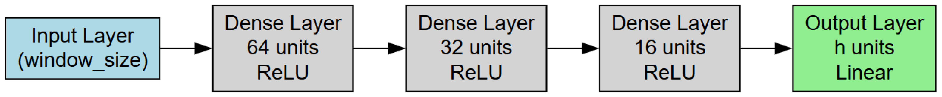
2. Neural Networks for Time Series Forecasting

Forecasting time series inherently involves distinct challenges due to the temporal correlation between successive data points, adding layers of complexity to predictive modeling. Neural network models, especially MLPs, have demonstrated substantial utility in effectively managing these complexities [34,35]. Among their principal strengths is resilience to noise and a powerful capability for modeling both linear and nonlinear dependencies without restrictive assumptions on the functional form of data relationships [36]. Their ability to approximate diverse nonlinear functions is particularly transformative within forecasting contexts.

Moreover, neural networks can readily adapt to arbitrary, pre-specified input and output dimensions, enabling efficient handling of multivariate inputs and multi-step-ahead forecasting scenarios, including the more challenging multivariate predictions [35]. Such versatility underscores the potential offered by feedforward neural network architectures for enhancing time series forecasting.

In this paper, we introduce a generic multi-step forecasting model based on MLPs, referred to as the Generic Multi-Step MLP (GMS-MLP), specifically designed for point forecasting in univariate time series data. The model is inspired by the implementation described in [6]. The primary objective of the GMS-MLP architecture is to predict the next h future values by leveraging historical data from a lookback window of length T.

The structure of the GMS-MLP consists of an input layer, three subsequent hidden layers employing ReLU activation functions, and a final output layer. Each component of this architecture is essential for identifying and capturing the intrinsic patterns and trends within the historical data. Bias parameters within the network are initially set to zero, while weights are initialized according to a widely adopted heuristic, sampling from a normal distribution with zero mean and a standard deviation defined by ${\displaystyle \frac{1}{\sqrt{n}}}$, where n denotes the size of the preceding layer [37].

The input layer of the proposed model is configured to match the size T, representing the length of the historical lookback period. Precisely, the lookback window $x_{T|t}\in {\mathbb{R}}^T=[y_{t-T+1},\dots ,y_t]$ consists of the T most recent observations up to the current time point t. In this design, each observation in the lookback window is treated independently as a distinct input feature. Selecting an appropriate window length T is vital, as it directly impacts the extent to which historical data influences the future predictions.

Figure 1 provides a visual depiction of the proposed GMS-MLP model’s architecture. This architecture is notably adaptable, allowing modifications to suit diverse forecasting scenarios. Specifically, the depicted example uses an input layer of size 10, corresponding to a scenario where $T=5h$ given a forecast horizon h of two future steps.

Table 1. Detailed architecture of the GMS-MLP model.

Layer (Type)	Output Shape	Params
Input Layer (Input)	(None, 10)	0
Dense 1 (ReLU)	(None, 64)	704
Dense 2 (ReLU)	(None, 32)	2080
Dense 3 (ReLU)	(None, 16)	528
Output Layer (Linear)	(None, 2)	34

complements the illustration by detailing each layer’s output shape and parameter count. In total, the GMS-MLP architecture comprises 3346 trainable parameters that are optimized during training.

Extending the previously introduced GMS-MLP framework for univariate time series forecasting, it becomes essential to address how forecast performance is assessed. Traditionally, the focus has been on measuring the accuracy of predictions. Given that the model parameters are optimized simultaneously over numerous time series through the minimization of a selected loss criterion, it is particularly important to choose scale-independent metrics—especially if no preprocessing is applied to the data beforehand.

An example of such a scale-invariant metric is the root mean squared scaled error (RMSSE), derived from the mean absolute scaled error (MASE) initially proposed by Hyndman and Koehler [38]. Specifically, the RMSSE for an individual input-output instance j, with forecasts generated from origin t, is formally defined by Van Belle et al. [4] as follows:

$$\mathrm{RMSSE}=\sqrt{{\displaystyle \frac{\frac{1}{h}{\sum }_{i=1}^h{(y_{t+i}-{\widehat{y}}_{t+i|t})}^2}{\frac{1}{T-1}{\sum }_{i=1}^{T-1}{(y_{t-i+1}-y_{t-i})}^2}}}.$$

(1)

In the above definition, h represents the forecast horizon, T indicates the length of the historical lookback window, $y_{t+i}$ signifies the true observed value at future time point $t+i$, and ${\widehat{y}}_{t+i|t}$ denotes the forecasted value at time $t+i$, conditioned upon information available up to time t. The denominator in the equation calculates the average squared difference between adjacent historical observations within the lookback period. This acts as a scaling factor, normalizing the error to eliminate dependence on the data’s scale.

Adopting RMSSE as the evaluation criterion allows the GMS-MLP model to be assessed and optimized based on forecasting accuracy independent of the magnitude of the underlying data. Consequently, this method significantly enhances the model’s flexibility, making it well-suited to various forecasting applications.

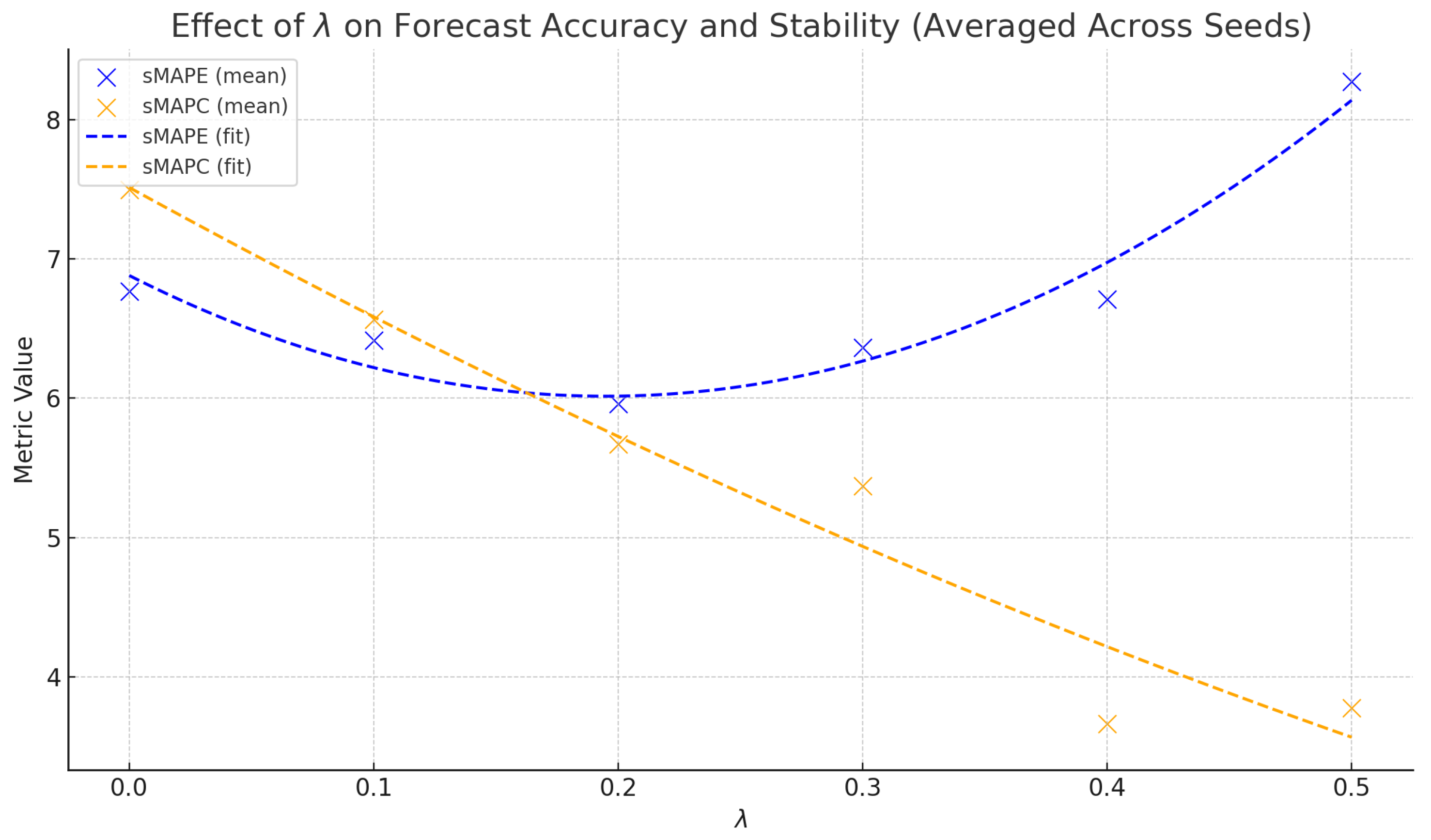
3. Improving the Stability of Multi-Step MLP Forecasts

To further enhance the stability of forecasts generated by the GMS-MLP model, an extended form of the standard RMSSE loss function is adopted Van Belle et al. [4]. This extension aims to address forecast variability by explicitly comparing predictions ${\widehat{y}}_j^{h|t}$ and ${\widehat{y}}_j^{h|t-1}$, which represent forecasts for the same input-output pair j originating at times t and $t-1$, respectively. Specifically, this comparison targets the overlapping forecast periods from $t+1$ to $t+h-1$. To systematically reduce differences in forecasts generated at consecutive origins, an instability penalty term is introduced into the loss function. Practically, this is accomplished by shifting the forecasting origin backward by one time step and utilizing this lagged input-output pair during the model’s training process.

A suitable measure for quantifying forecast instability, called the root mean squared scaled change (RMSSC), is introduced. This metric is scale-independent and structurally analogous to RMSSE. For a given sample j with forecasting origins at $t-1$ and t, RMSSC is formally defined as follows:

$$\mathrm{RMSSC}=\sqrt{{\displaystyle \frac{\frac{1}{h-1}{\sum }_{i=1}^{h-1}{\left({\widehat{y}}_{t+i|t}-{\widehat{y}}_{t+i|t-1}\right)}^2}{\frac{1}{T-1}{\sum }_{i=1}^{T-1}{\left(y_{t-i+1}-y_{t-i}\right)}^2}}}.$$

(2)

Within this definition, h denotes the forecasting horizon, T signifies the length of the historical lookback period, ${\widehat{y}}_{t+i|t}$ refers to the forecasted observation at time $t+i$ conditioned on data available up to time t, and ${\widehat{y}}_{t+i|t-1}$ represents the corresponding prediction at time $t+i$ conditioned on data available up to time $t-1$. The denominator calculates the mean squared differences between consecutive historical observations within the lookback window, acting as a normalization term to preserve the scale-independence of the metric.

The core aim is to concurrently minimize both forecast error and forecast instability. Traditionally, forecasting techniques for time series data have prioritized accuracy, assuming that enhancements in predictive accuracy typically outweigh the costs linked with frequently updating forecasts [4]. Nevertheless, simultaneously emphasizing both accuracy and stability can potentially yield higher-quality, more reliable predictions.

To achieve this objective, we propose a composite loss function that explicitly integrates the forecast instability term:

$$L\left(\lambda \right)=(1-\lambda )·L_{\mathrm{RMSSE}}+\lambda ·L_{\mathrm{RMSSC}},$$

(3)

where $L\left(\lambda \right)$ represents the combined loss function employed in the enhanced multi-step MLP (EMS-MLP) framework. The hyperparameter $\lambda$ serves as a balancing factor, regulating the trade-off between prediction accuracy (as measured by RMSSE) and forecast stability (as quantified by RMSSC). Through varying $\lambda$, this study aims to explore the extent to which forecast stability can be improved without adversely affecting overall prediction accuracy.

4. Dataset Construction

The dataset used in this study originates from the Global Carbon Project’s (GCP) “Global Carbon Budget (2024)” release, which has undergone extensive processing by Our World in Data [5]. The original dataset spans from 1750 to 2023, measured in tonnes of CO₂ (excluding land-use change). It includes annual territorial emissions for countries and regions worldwide, with further details provided in the metadata from the GCP.

For our analysis, we generated an updated version of this dataset by removing all entries with zero annual CO₂ emissions. Consequently, the updated dataset better reflects observed emission patterns across time without introducing spurious zeros.

4.1. Dataset Overview and Key Details

• Temporal Coverage: 1750–2023 (annual frequency).
• Geographical Coverage: Multiple countries and regions worldwide.
• Indicator: Annual total emissions of CO₂ (excluding land-use change), measured in tonnes.
• Source: Global Carbon Budget (2024) with major processing by Our World in Data.
• Final Processing Date: 21 November 2024.
• Unit: Tonnes of CO₂.
• Data Modifications:
  • Conversion from tonnes of carbon to tonnes of CO₂ using a factor of 3.664, as documented by Our World in Data.
  • Removal of zero-emission entries from annual records.
  • Standardization of country/region naming conventions and alignment of date ranges where applicable.

4.2. Summary Statistics

To illustrate the structure and variability of the updated dataset, we aggregated time-series data for each country or region into individual emission trajectories (one per series). After filtering out zero values, the following summary applies:

• No. of series: 244 (For example, each series corresponds to a distinct country/region that has non-zero emissions data over some portion of 1750–2023.)
• Min. length: 20 years (Reflecting countries with relatively few non-zero emission records, often due to late starts in industrial activity or incomplete historical data.)
• Max. length: 274 years (Indicating that some regions/countries have continuous non-zero records dating back to the mid-18th century.)
• Mean length: 114.8 years (The average count of non-zero annual entries per series.)
• Std. dev. length: 57.2 years (Highlighting moderate variability in the number of available non-zero data points across countries.)

Table 2. Summary statistics of the updated dataset.

Statistic	Value	Description
No. of series	244	Distinct country/region time series
Min. length	20	Fewest non-zero annual records
Max. length	274	Most consecutive non-zero annual records
Mean length	114.8	Average series length
Std. dev. length	57.2	Variability in series lengths

summarizes these core statistics at a glance.

4.3. Distribution of Time Series Lengths

Figure 2 provides an illustrative distribution of time series lengths (i.e., the number of non-zero emission points per country or region). This histogram indicates that while many series cluster around mid-range lengths (100–200 years), a subset of countries has emission records spanning well over two centuries. Conversely, some countries or regions feature only a few decades of documented non-zero emissions, suggesting shorter industrial histories or gaps in earlier records.

4.4. Additional Context and Considerations

• Exclusions: The dataset excludes emissions from international aviation and shipping, and does not account for net imports or exports of embedded carbon in traded goods.
• Historical vs. Current Comparisons: Longer series provide valuable historical context, enabling trend analysis from the dawn of the Industrial Revolution to the present. Shorter series can still inform recent trajectories but may lack the breadth for extended historical comparisons.

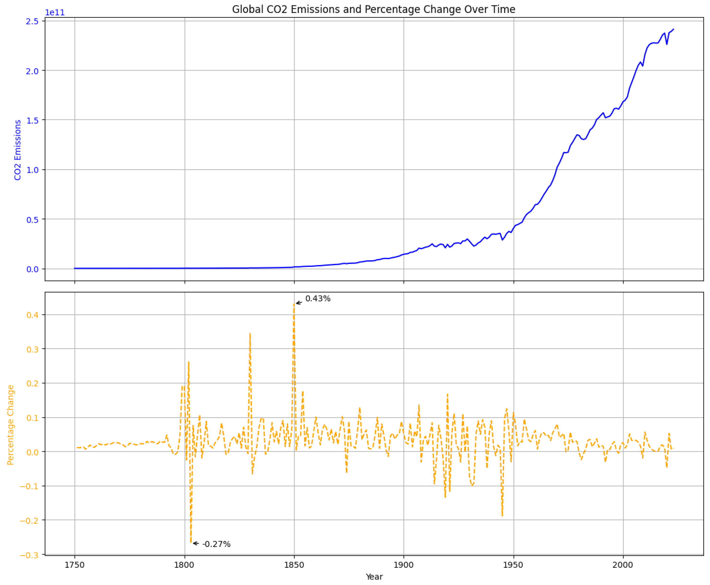
4.5. CO₂ Emissions over Time: Absolute and Relative Change

Figure 3 presents a two-part visualization illustrating global CO₂ emissions over time. The top subplot displays the total annual CO₂ emissions in blue, capturing the aggregate emissions recorded each year. In contrast, the bottom subplot emphasizes the year-over-year percentage change in emissions, represented by a red dashed line. To highlight key moments in the data, annotations mark the years with the most significant positive and negative percentage changes.

The overall trend in global CO₂ emissions reveals a clear upward trajectory, reflecting a sustained increase in emissions over the observed period. This long-term growth aligns with industrialization, population growth, and increased energy consumption worldwide. Notably, the year 1850 witnessed the largest positive year-over-year change in emissions, with an increase of approximately 0.43%. Conversely, the most significant decline occurred in 1803, marked by a decrease of about 0.27%. These inflection points may correspond to major historical or economic developments that influenced emission patterns.

Despite the overall upward trend, emissions show notable variability, reflecting alternating periods of acceleration and deceleration driven by economic, technological, and policy factors.

The two subplots complement each other: sharp increases in total emissions (top) align with peaks in percentage change (bottom), while stagnation or decline appears as negative changes. Together, they reveal both the scale and dynamics of global CO₂ emissions, clarifying historical trends and variability.

4.6. Relevance to Modeling and Forecasting

These data form the foundation for our subsequent modeling and forecasting work, enabling us to train algorithms on consistent, non-zero emission series spanning multiple geographies and timeframes. By explicitly removing spurious zero observations, we mitigate distortions in model training. The broad range of time series lengths (20 to 274 years) highlights the need for forecasting techniques that can adapt to varying historical depths and data quality, underscoring the significance of robust, flexible, and domain-aware modeling approaches.

5. Experimental Design and Methodology

This section outlines the experimental framework used to train and evaluate the forecasting models. We begin by describing the data splitting strategy, which structures the time series into training, validation, and test sets. We then detail the hyperparameter configuration, focusing on the role of the stability parameter $\lambda$ in the EMS-MLP model. The implementation and training procedures are described next, including optimization settings and early stopping criteria. Finally, we explain the evaluation scheme, which relies on rolling-origin forecasts to assess model performance, and introduce the Average Forecast Strategy (AFS) as a baseline benchmark.

5.1. Data Splitting Strategy

The dataset is partitioned into training, validation, and test sets. For each individual time series, the test set comprises the last three observations, while the validation set includes the three observations immediately preceding the test set. The remaining portion of the series is allocated to the training set. The forecasting model predicts the next h time steps (in this case, $h=2$ for two-step-ahead forecasts). Throughout the experiments, a lookback window of length $T=10$ is employed to construct the input sequences for the model.

5.2. Hyperparameter Configuration

In the EMS-MLP model proposed in this study, hyperparameter tuning is focused exclusively on a single parameter, $\lambda$. This hyperparameter governs the contribution of the forecast instability component in the optimization objective, thereby influencing the stability and accuracy of the generated forecasts.

All other hyperparameters are retained at their optimized settings as used in the GMS-MLP model. This consistency ensures that performance comparisons between the EMS-MLP and GMS-MLP variants isolate the effect of $\lambda$. Notably, setting $\lambda =0$ corresponds to the GMS-MLP configuration.

5.3. Implementation and Training Procedure

Both the GMS-MLP and EMS-MLP models are implemented using the Keras [39,40] deep learning framework. The training process employs the Adam optimizer [41] with default settings. To address potential issues of overfitting and underfitting, an early stopping mechanism is utilized. This approach allows the model to train for a large number of epochs while automatically halting the process when performance on the validation set ceases to improve.

5.4. Evaluation Scheme

Standard evaluation methods that assume forecasts from a single origin do not align well with the objectives of this study, particularly in assessing forecast stability. To address this challenge, a rolling forecasting origin evaluation strategy is adopted. In this approach, the forecasting origin is successively updated, and forecasts are generated from each updated point. This dynamic evaluation method better reflects real-world scenarios where predictions are repeatedly updated as new data becomes available.

Although RMSSE is employed as the validation loss metric during training, the evaluation of forecast accuracy and stability is conducted using the symmetric mean absolute percentage error (sMAPE) and the symmetric mean absolute percentage change (sMAPC) metrics. These metrics are chosen for their interpretability and practical relevance, despite the fact that sMAPE is not used during training due to its sensitivity to numerical instability, as highlighted by Van Belle et al. [4].

sMAPE is formulated as follows:

$$\mathrm{sMAPE}={\displaystyle \frac{200}{h}}\sum _{i=1}^h{\displaystyle \frac{|y_{t+i}-{\widehat{y}}_{t+i|t}|}{|y_{t+i}|+|{\widehat{y}}_{t+i|t}|}}$$

In this equation, $y_{t+i}$ denotes the observed value of the time series at time $t+i$, while ${\widehat{y}}_{t+i|t}$ represents the forecast for period $t+i$ made at the forecasting origin t. The parameter h specifies the maximum forecast horizon. To evaluate the model’s performance across various forecasting origins, the average of the computed sMAPE values is used.

While sMAPE effectively quantifies forecast accuracy by comparing predictions with observed values, it does not assess the stability of forecasts over time. To address this limitation, Van Belle et al. [4] introduced the symmetric mean absolute percentage change (sMAPC), a metric specifically designed to measure instability in rolling-origin forecasts.

For consecutive forecasting origins $t-1$ and t, the sMAPC over one- to h-step-ahead forecasts is defined as:

$$\mathrm{sMAPC}={\displaystyle \frac{200}{(h-1)}}\sum _{i=1}^{h-1}{\displaystyle \frac{|{\widehat{y}}_{t+i|t}-{\widehat{y}}_{t+i|t-1}|}{|{\widehat{y}}_{t+i|t}|+|{\widehat{y}}_{t+i|t-1}|}}$$

The fundamental difference between sMAPE and sMAPC lies in their comparative approach: while sMAPE compares forecasts with the actual observed values, sMAPC compares forecasts from adjacent origins. This makes sMAPC particularly useful for assessing the stability of forecasts over time.

To evaluate the overall instability across multiple forecasting origins, the mean of the computed sMAPC values is calculated. This averaging process ensures a comprehensive assessment of stability over the entire forecasting period, thereby providing insights into the consistency of the model’s performance when facing varying forecasting origins.

In this study, the Average Forecast Strategy (AFS) is employed as a benchmark to evaluate the performance of the proposed forecasting models. AFS offers a simple and intuitive baseline: it predicts future values by computing the mean of all historical observations available up to the forecast origin. This approach requires minimal assumptions about the data, making it suitable for general-purpose benchmarking.

If we denote the observed time series as $y_1,y_2,\dots ,y_t$, the AFS produces a forecast ${\widehat{y}}_{t+h|t}$ for a future time point $t+h$ (with h being the forecast horizon) using the following formula:

$${\widehat{y}}_{t+h|t}=\overline{y}={\displaystyle \frac{y_1+y_2+\dots +y_t}{t}}$$

(4)

Here, ${\widehat{y}}_{t+h|t}$ denotes the forecast of $y_{t+h}$ based on information available up to time t, and $\overline{y}$ is the mean of all past observations. The AFS is not tailored to short-term trends, seasonality, or sudden changes in the series; rather, it provides a stable reference point for assessing whether more sophisticated models offer added predictive value. If a model consistently outperforms AFS across various metrics, it can be considered skillful.

This benchmark is particularly useful in time series forecasting studies, as it helps determine whether model complexity yields a meaningful improvement over a simple historical average.

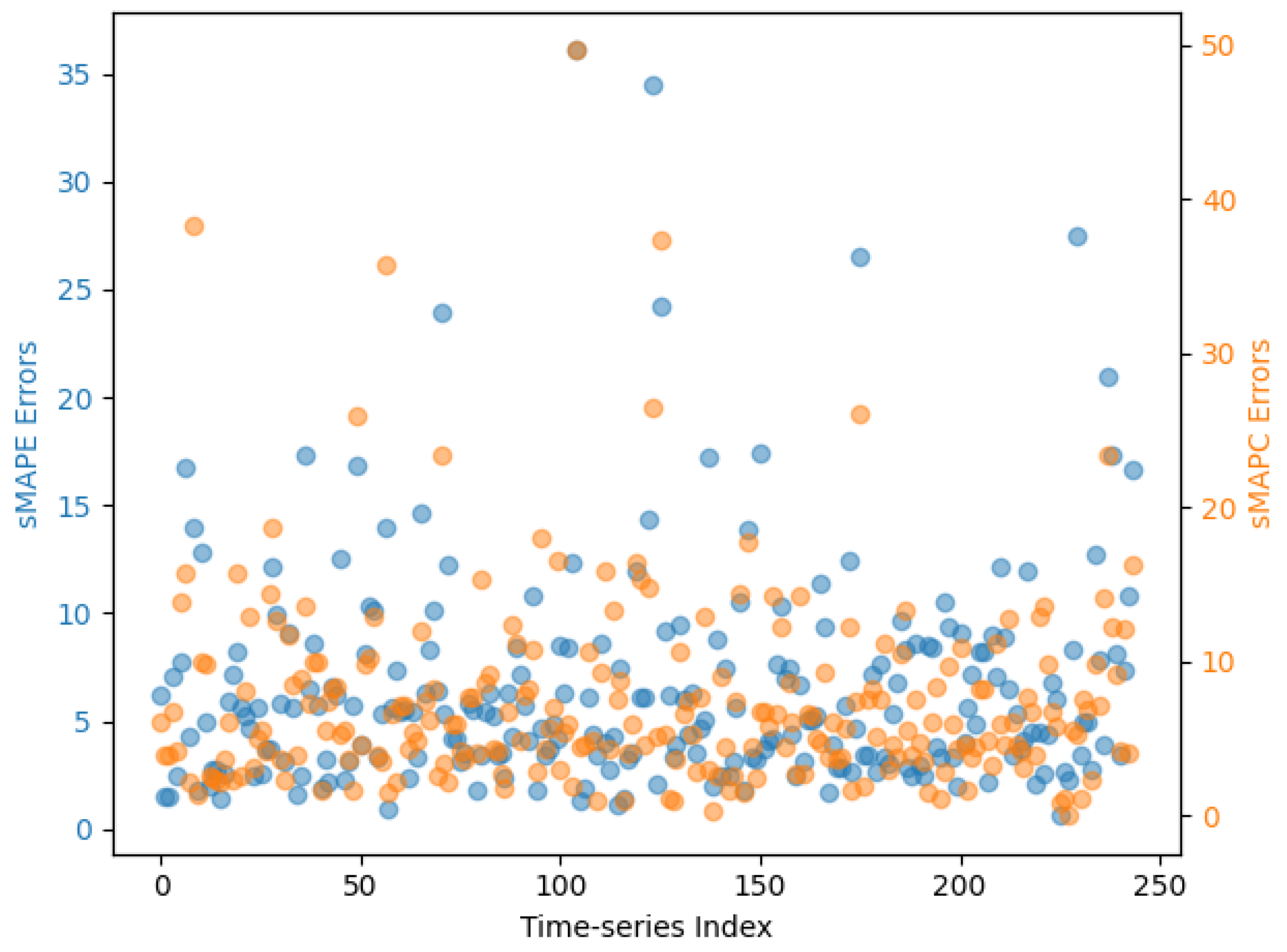
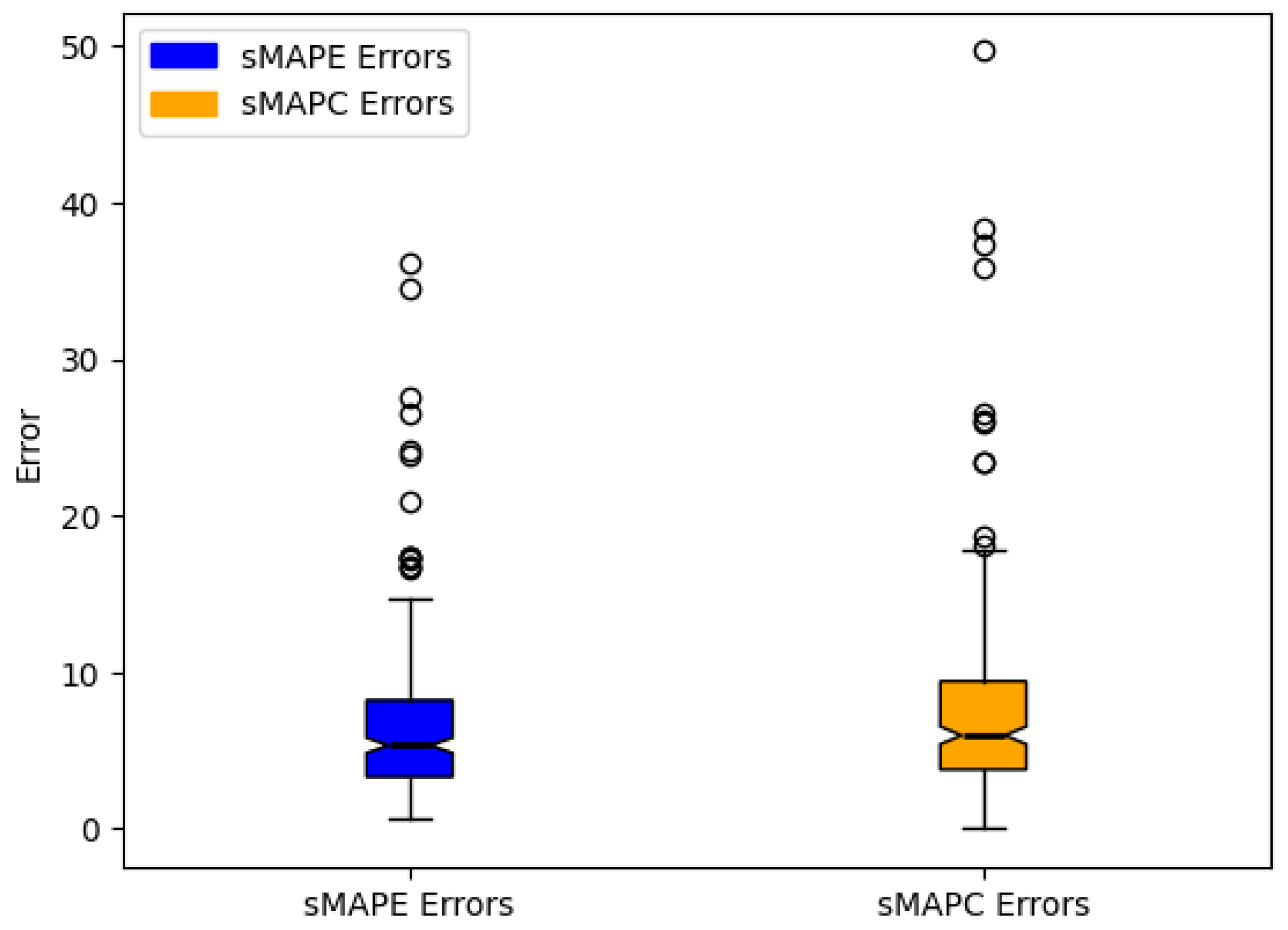
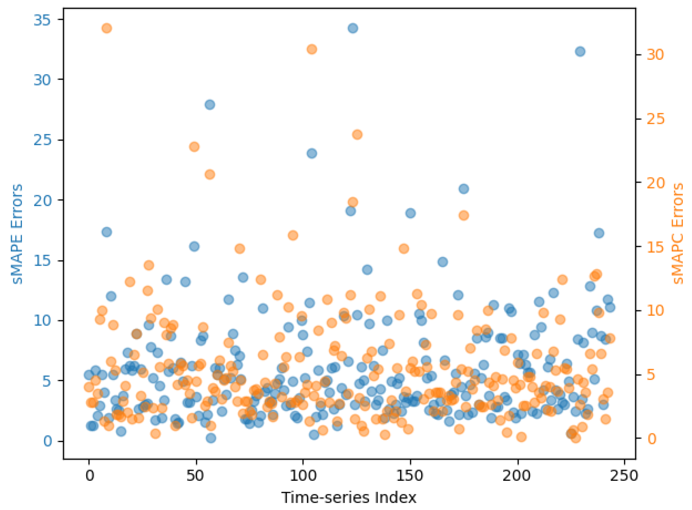
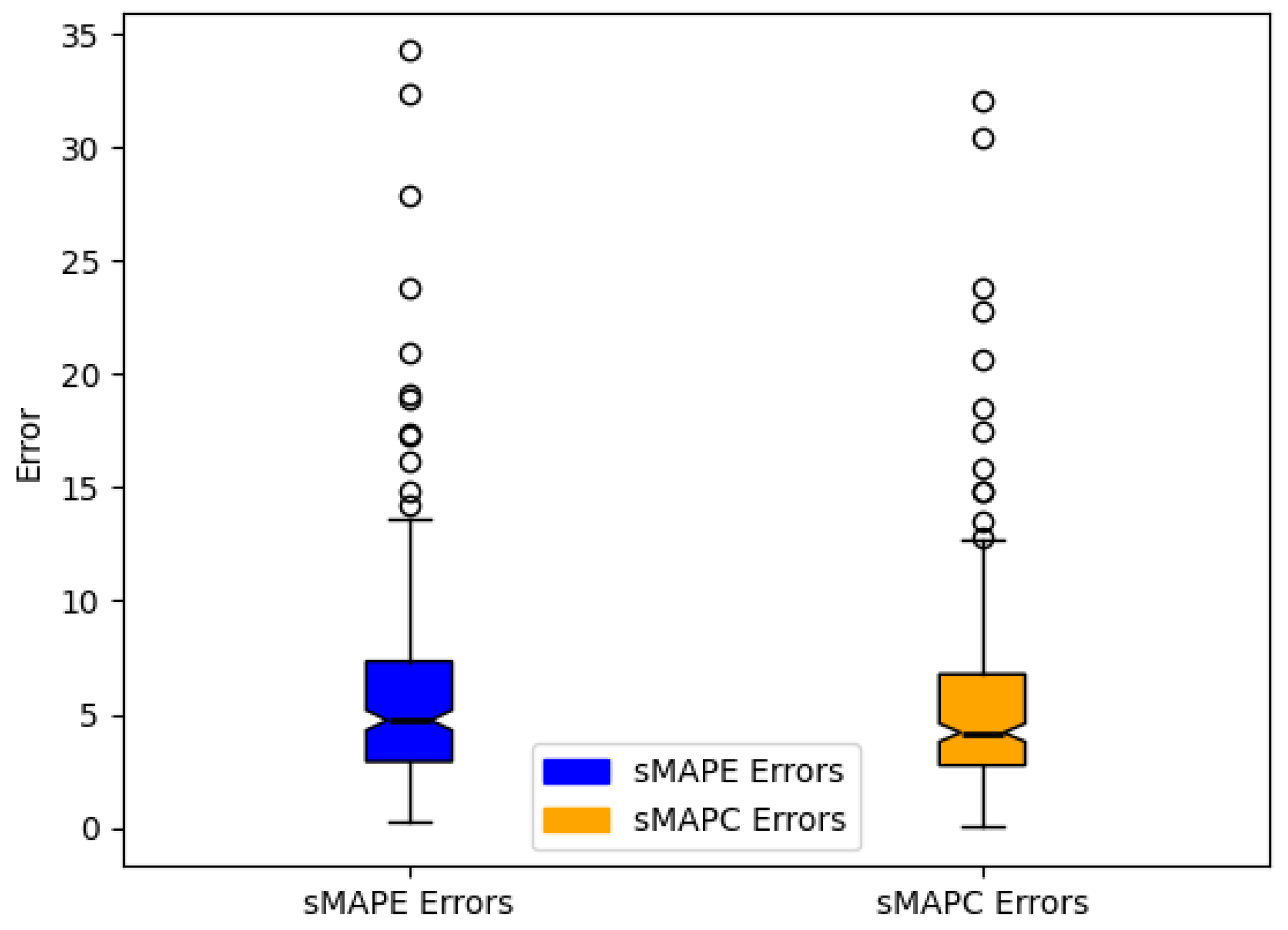
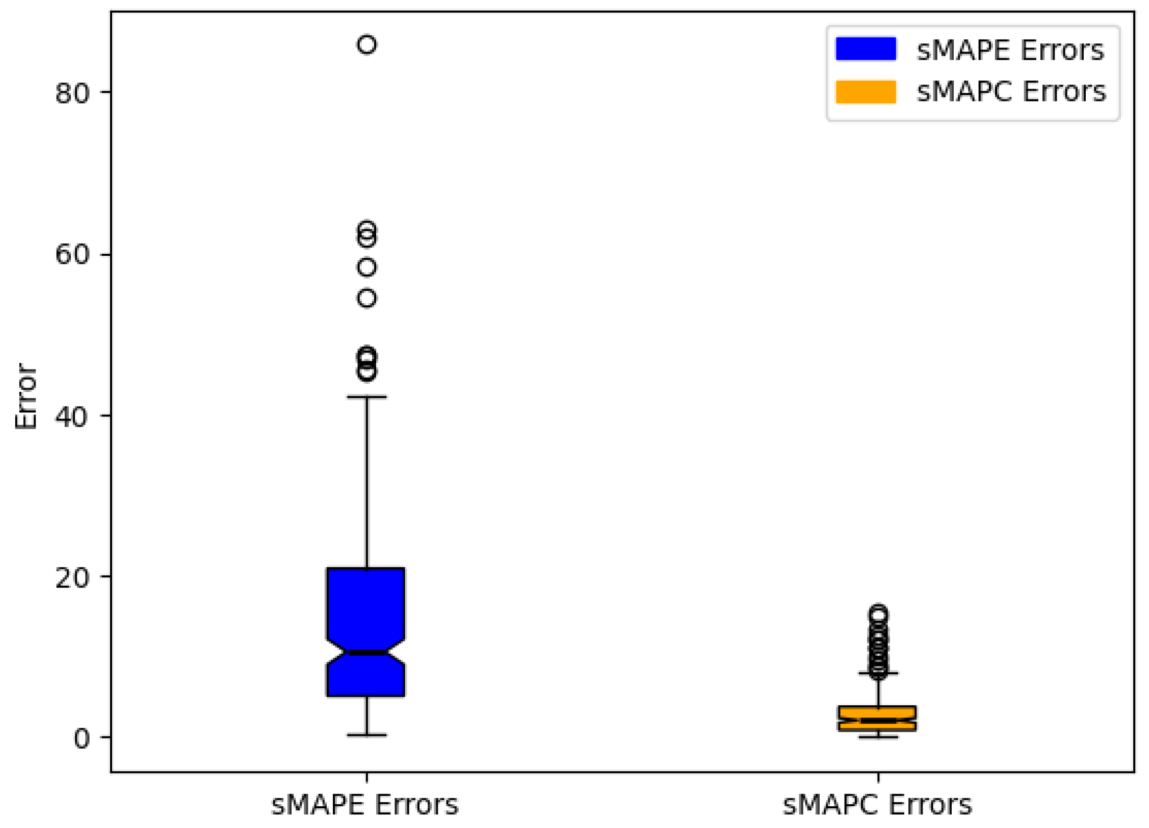
6. Results and Discussion

To quantitatively evaluate the accuracy of the forecasting models, we rely on two previously defined performance measures: sMAPE and sMAPC. These measures are applied consistently across all experiments.

For each individual time series, both metrics are computed by averaging over multiple forecasting origins. This approach provides a robust estimate of performance over time. Subsequently, the values are aggregated again by averaging across all time series to yield an overall model performance score.

In this study, we focus on forecasts extending one to two years ahead, corresponding to two-step-ahead forecasts for each time series in the test set. Specifically, for each series, two forecast sets are generated from two consecutive forecasting origins.

Three models are evaluated: the GMS-MLP, the EMS-MLP, and AFS, which serves as a reference point. To visualize forecasting accuracy and stability, scatter plots are used to display the sMAPE and sMAPC values for each individual time series. These highlight how performance varies across different data instances. In addition, box plots are provided to summarize the statistical distribution of errors for each model, offering a more compact view of overall performance dispersion.

The corresponding visualizations are shown in Figure 4, Figure 5, Figure 6, Figure 7, Figure 8 and Figure 9, where each figure focuses on a specific combination of model and metric. Together, these plots facilitate both detailed and comparative analysis of the models’ forecasting capabilities.

To gain deeper insights into the forecasting performance of each model, we summarize the sMAPE and sMAPC errors using descriptive statistics in

Table 3. Statistics for sMAPE and sMAPC errors.

	sMAPE			sMAPC
	Mean	Std. dev.	Median	Mean	Std. dev.	Median
GMS-MLP	6.55	5.16	5.33	7.57	6.41	5.97
EMS-MLP	5.92	4.80	4.73	5.46	4.52	4.19
AFS	14.49	12.96	10.58	2.85	2.83	2.09

. These metrics not only reflect the overall accuracy of the forecasts (as indicated by mean and median values) but also provide a measure of stability through the reported standard deviations. Lower mean and median values suggest better predictive performance, while smaller standard deviations indicate more consistent and reliable forecasts across the time series.

An analysis of the forecasting outcomes in Table 3 clearly indicates that the EMS-MLP model surpasses the GMS-MLP in overall forecasting accuracy. Notably, the EMS-MLP attains a lower mean sMAPE of 5.92, in contrast to 6.55 achieved by the GMS-MLP. Both models significantly outperform the baseline AFS, which exhibits a considerably higher sMAPE of 14.49.

When assessing the stability of the forecasts with the sMAPC metric, the EMS-MLP continues to outperform the GMS-MLP, achieving a lower mean sMAPC of 5.46 versus 7.57, thus indicating less forecast variability. A one-tailed permutation test based on 10,000 random label swaps shows that the accompanying reduction in sMAPC is favorable but not statistically significant at the 5% level ($p=0.096$), whereas the same test applied to the paired sMAPE errors confirms a significant accuracy gain for EMS MLP ($p=0.047$). Interestingly, the AFS baseline attains the numerically lowest sMAPC of 2.85; however, this apparent stability is offset by markedly inferior accuracy, as reflected in its much higher sMAPE. This behaviour is consistent with the baseline’s bias toward overly smooth predictions that ignore short-term dynamics.

The comparison between EMS-MLP and GMS-MLP also reveals that selecting appropriate values for the regularization parameter $\lambda$—specifically $\lambda =0.2$ in this case—can meaningfully enhance forecast stability without compromising accuracy. The EMS-MLP’s simultaneous improvements in both sMAPE and sMAPC support the hypothesis that incorporating a forecast instability term into the loss function acts as a task-specific regularization mechanism. This adjustment encourages the model to produce more stable forecasts while preserving its ability to learn temporal patterns effectively. While our experimental design focuses on isolating the impact of the stability-aware loss by comparing EMS-MLP with its baseline variant and a naive average strategy, future work will extend this evaluation to include established models such as LSTM, Prophet, and Transformer-based architectures to further validate the generalizability and competitiveness of the proposed approach.

Figure 10 presents the impact of the regularization parameter $\lambda$ on forecasting performance, evaluated using the sMAPE and sMAPC metrics. The results are averaged across five distinct random seeds to ensure robustness. Each point on the plot represents the mean metric value across these runs, while the dashed lines denote second-degree polynomial fits, capturing the overall trend for each metric.

As shown in the figure, the sMAPE curve exhibits a U-shaped pattern, suggesting that forecast accuracy improves with small increases in $\lambda$, reaching a minimum around $\lambda =0.2$, before deteriorating at higher values. This trend implies that a moderate regularization strength helps reduce overfitting and encourages more accurate forecasting. However, excessively high values of $\lambda$ may overly constrain the model, leading to underfitting and reduced accuracy.

In contrast, the sMAPC values decrease consistently as $\lambda$ increases. This monotonic decline indicates that higher regularization effectively enhances the temporal smoothness and stability of the forecasted time series. The lowest sMAPC is observed at $\lambda =0.5$, confirming that stronger penalties on forecast instability contribute significantly to reducing fluctuation and noise in predictions.

These dual trends highlight the trade-off between accuracy and stability in regularized forecasting models. Importantly, the region around $\lambda =0.2$ appears to offer an optimal balance, simultaneously achieving low forecast error and substantial gains in stability. This supports the idea that integrating a forecast instability penalty in the loss function can serve as a task-specific regularization mechanism, enhancing both predictive performance and temporal coherence.

In summary, introducing an instability penalty into our multi-step MLP yields a clear win: at the optimal weight $\lambda =0.2$, the EMS-MLP cuts average error (sMAPE) from 6.55% to 5.92% and reduces forecast jitter (sMAPC) by over 25% relative to the baseline GMS-MLP—outperforming both the standard MLP and a stable but inaccurate historical average. This sweet spot shows that accuracy and stability need not trade off: by tuning $\lambda$, we produce CO₂ projections that are both precise and consistent, giving policymakers reliable, actionable forecasts.

Beyond numerical improvements, the simultaneous enhancement in forecast accuracy and temporal stability achieved by the EMS-MLP model carries direct and significant implications for policy and environmental planning. National inventory agencies and climate-model ensembles increasingly rely on reliable short-term CO₂ forecasts to set carbon-budget checkpoints and inform timely mitigation strategies. Unstable or imprecise predictions can lead to misaligned or delayed actions, undermining effective climate responses. By reducing forecast error and dampening volatility, the EMS-MLP offers policymakers more dependable, actionable insights suitable for regular progress tracking, emissions-trading systems, and early-warning mechanisms for target slippage. Taken together, these attributes position the EMS-MLP as a practical tool for integrating precise CO₂ projections into policy dashboards, climate-finance risk models, and regional decarbonization strategies.

7. Conclusions

In this work, we have demonstrated that integrating a forecast-instability penalty into a multi-step MLP framework yields CO₂ emissions projections that are both accurate and temporally stable. By striking an optimal balance at a regularization strength of $\lambda =0.2$, our EMS-MLP model reduces forecast variability without sacrificing predictive performance, outperforming both the GMS-MLP and a conventional baseline. These improvements are particularly relevant for monitoring progress under the Paris Agreement, where consistent, reliable long-term emissions estimates are essential for assessing national commitments and global temperature targets. Moreover, our approach directly supports Sustainable Development Goal 13 (Climate Action) by providing decision makers with robust tools to evaluate policy scenarios and to design adaptive mitigation strategies. We believe that stability-aware forecasting can become an indispensable component of environmental policy planning, enabling stakeholders to base critical decisions on projections that are not only precise but also resilient to short-term data fluctuations.

A key next step is to develop an adaptive regularisation scheme that automatically tunes the instability penalty $\lambda$ in real time, allowing the model to adjust to evolving emission patterns or abrupt regime shifts. Embedding the EMS–MLP in an operational dashboard with live data feeds and automated recalibration would make it immediately actionable for policy makers tracking Paris-Agreement commitments. When higher-frequency (monthly or daily) data become available, the look-back window T and the stability weight $\lambda$ will need to be re-tuned to capture sub-annual dynamics. We also plan to extend the stability-aware loss to a multi-task setting so that CO₂, CH₄, and N₂O can be forecast jointly. Finally, expanding the framework to other greenhouse gases and disaggregated sectoral forecasts will further broaden its applicability to climate-risk assessment and mitigation planning.

References

1. Eiglsperger, J.; Haselbeck, F.; Grimm, D.G. Foretis: A comprehensive time series forecasting framework in python. Mach. Learn. Appl. 2023, 12, 100467. [Google Scholar] [CrossRef]
2. Lara-Benítez, P.; Carranza-García, M.; Riquelme, J.C. An experimental review on deep learning architectures for time series forecasting. Int. J. Neural Syst. 2021, 31, 2130001. [Google Scholar] [CrossRef]
3. Steele, D.C. The nervous MRP system: How to do battle. Prod. Inventory Manag. 1975, 16, 83–89. [Google Scholar]
4. Van Belle, J.; Crevits, R.; Verbeke, W. Improving forecast stability using deep learning. Int. J. Forecast. 2023, 39, 1333–1350. [Google Scholar] [CrossRef]
5. Global Carbon Project. Global Carbon Budget (2024)—Annual CO2 Emissions. Processed by Our World in Data. 2024. Available online: https://www.globalcarbonproject.org/ (accessed on 1 May 2025).
6. Alsharkawi, A. Improving Stability in Univariate Time Series Forecasting Using Multi-Layer Perceptron Neural Network. Master’s Thesis, KU Leuven, Faculty of Engineering Technology, Leuven, Belgium, 2023. [Google Scholar]
7. Makridakis, S.; Hibon, M. The m3-competition: Results, conclusions and implications. Int. J. Forecast. 2000, 16, 451–476. [Google Scholar] [CrossRef]
8. Makridakis, S.; Spiliotis, E.; Assimakopoulos, V. The m4 competition: 100,000 time series and 61 forecasting methods. Int. J. Forecast. 2020, 36, 54–74. [Google Scholar] [CrossRef]
9. Dengerud, E.O. Global Models for Time Series Forecasting with Applications to Zero-Shot Forecasting. Master’s Thesis, Norwegian University of Science and Technology, Trondheim, Norway, 2021. [Google Scholar]
10. Januschowski, T.; Kolassa, S. A classification of business forecasting problems. In Business Forecasting: The Emerging Role of Artificial Intelligence and Machine Learning; John Wiley & Sons: Hoboken, NJ, USA, 2021; p. 171. [Google Scholar]
11. Akan, T. Forecasting the future of carbon emissions by business confidence. Appl. Energy 2025, 382, 125146. [Google Scholar] [CrossRef]
12. Han, T.T.T.; Lin, C.Y. Exploring long-run CO2 emission patterns and the environmental kuznets curve with machine learning methods. Innov. Green Dev. 2025, 4, 100195. [Google Scholar] [CrossRef]
13. Jha, R.; Jha, R.; Islam, M. Forecasting us data center CO2 emissions using ai models: Emissions reduction strategies and policy recommendations. Front. Sustain. 2025, 5, 1507030. [Google Scholar] [CrossRef]
14. Zhong, W.; Zhai, D.; Xu, W.; Gong, W.; Yan, C.; Zhang, Y.; Qi, L. Accurate and efficient daily carbon emission forecasting based on improved arima. Appl. Energy 2024, 376, 124232. [Google Scholar] [CrossRef]
15. Wu, B.; Zeng, H.; Wang, Z.; Wang, L. Interpretable short-term carbon dioxide emissions forecasting based on flexible two-stage decomposition and temporal fusion transformers. Appl. Soft Comput. 2024, 159, 111639. [Google Scholar] [CrossRef]
16. Nguyen, V.G.; Duong, X.Q.; Nguyen, L.H.; Nguyen, P.Q.P.; Priya, J.C.; Truong, T.H.; Le, H.C.; Pham, N.D.K.; Nguyen, X.P. An extensive investigation on leveraging machine learning techniques for high-precision predictive modeling of CO2 emission. Energy Sources Part A Recover. Util. Environ. Eff. 2023, 45, 9149–9177. [Google Scholar]
17. Hu, Y.; Wang, B.; Yang, Y.; Yang, L. An enhanced particle swarm optimization long short-term memory network hybrid model for predicting residential daily CO2 emissions. Sustainability 2024, 16, 8790. [Google Scholar] [CrossRef]
18. Ding, S.; Zhang, H. Forecasting chinese provincial CO2 emissions: A universal and robust new-information-based grey model. Energy Econ. 2023, 121, 106685. [Google Scholar] [CrossRef]
19. Ding, S.; Shen, X.; Zhang, H.; Cai, Z.; Wang, Y. An innovative data-feature-driven approach for CO2 emission predictive analytics: A perspective from seasonality and nonlinearity characteristics. Comput. Ind. Eng. 2024, 192, 110195. [Google Scholar] [CrossRef]
20. An, Y.; Dang, Y.; Wang, J.; Zhou, H.; Mai, S.T. Mixed-frequency data sampling grey system model: Forecasting annual CO2 emissions in China with quarterly and monthly economic-energy indicators. Appl. Energy 2024, 370, 123531. [Google Scholar] [CrossRef]
21. Hu, Y.; Wang, B.; Yang, Y.; Yang, L. A novel approach for predicting CO2 emissions in the building industry using a hybrid multi-strategy improved particle swarm optimization–long short-term memory model. Energies 2024, 17, 4379. [Google Scholar] [CrossRef]
22. Adegboye, O.R.; Ülker, E.D.; Feda, A.K.; Agyekum, E.B.; Mbasso, W.F.; Kamel, S. Enhanced multi-layer perceptron for CO2 emission prediction with worst moth disrupted moth fly optimization (wmfo). Heliyon 2024, 10, e31850. [Google Scholar] [CrossRef] [PubMed]
23. Ajala, A.A.; Adeoye, O.L.; Salami, O.M.; Jimoh, A.Y. An examination of daily CO2 emissions prediction through a comparative analysis of machine learning, deep learning, and statistical models. Environ. Sci. Pollut. Res. 2025, 32, 2510–2535. [Google Scholar] [CrossRef]
24. Zhou, Z.; Yu, L.; Wang, Y.; Tian, Y.; Li, X. Innovative approach to daily carbon dioxide emission forecast based on ensemble of quantile regression and attention bilstm. J. Clean. Prod. 2024, 460, 142605. [Google Scholar] [CrossRef]
25. Li, Y.; Wang, Z.; Liu, S. Enhance carbon emission prediction using bidirectional long short-term memory model based on text-based and data-driven multimodal information fusion. J. Clean. Prod. 2024, 471, 143301. [Google Scholar] [CrossRef]
26. Filelis-Papadopoulos, C.K.; Kirshner, S.N.; O’Reilly, P. Sustainability with limited data: A novel predictive analytics approach for forecasting CO2 emissions. Inf. Syst. Front. 2024, 27, 1227–1251. [Google Scholar] [CrossRef]
27. Mekouar, Y.; Saleh, I.; Karim, M. Greennav: Spatiotemporal prediction of CO2 emissions in paris road traffic using a hybrid cnn-lstm model. Network 2025, 5, 2. [Google Scholar] [CrossRef]
28. Yuan, H.; Ma, X.; Ma, M.; Ma, J. Hybrid framework combining grey system model with gaussian process and stl for CO2 emissions forecasting in developed countries. Appl. Energy 2024, 360, 122824. [Google Scholar] [CrossRef]
29. Sapnken, F.E.; Hong, K.R.; Noume, H.C.; Tamba, J.G. A grey prediction model optimized by meta-heuristic algorithms and its application in forecasting carbon emissions from road fuel combustion. Energy 2024, 302, 131922. [Google Scholar] [CrossRef]
30. Zhu, P.; Zhang, H.; Shi, Y.; Xie, W.; Pang, M.; Shi, Y. A novel discrete conformable fractional grey system model for forecasting carbon dioxide emissions. Environ. Dev. Sustain. 2025, 27, 13581–13609. [Google Scholar] [CrossRef]
31. Xie, Y.; Liu, L.; Han, Z.; Zhang, J. Mscl-attention: A multi-scale convolutional long short-term memory (lstm) attention network for predicting CO2 emissions from vehicles. Sustainability 2024, 16, 8547. [Google Scholar] [CrossRef]
32. Wang, H.; Wei, Z.; Fang, T.; Xie, Q.; Li, R.; Fang, D. Carbon emissions prediction based on the giowa combination forecasting model: A case study of China. J. Clean. Prod. 2024, 445, 141340. [Google Scholar] [CrossRef]
33. Wang, Y.; Zhao, X.; Zhu, W.; Yin, Y.; Bi, J.; Gui, R. Forecasting carbon dioxide emissions in chongming: A novel hybrid forecasting model coupling gray correlation analysis and deep learning method. Environ. Monit. Assess. 2024, 196, 941. [Google Scholar] [CrossRef] [PubMed]
34. Hyndman, R.J.; Athanasopoulos, G. Forecasting: Principles and Practice; OTexts, 2018. [Google Scholar]
35. Zhang, G.; Patuwo, B.E.; Hu, M.Y. Forecasting with artificial neural networks: The state of the art. Int. J. Forecast. 1998, 14, 35–62. [Google Scholar] [CrossRef]
36. Hornik, K.; Stinchcombe, M.; White, H. Multilayer feedforward networks are universal approximators. Neural Netw. 1989, 2, 359–366. [Google Scholar] [CrossRef]
37. Glorot, X.; Bengio, Y. Understanding the difficulty of training deep feedforward neural networks. In Proceedings of the Thirteenth International Conference on Artificial Intelligence and Statistics, JMLR Workshop and Conference Proceedings, Sardinia, Italy, 13–15 May 2010; pp. 249–256. [Google Scholar]
38. Hyndman, R.J.; Koehler, A.B. Another look at measures of forecast accuracy. Int. J. Forecast. 2006, 22, 679–688. [Google Scholar] [CrossRef]
39. Chollet, F.; Others. Keras. 2015. Available online: https://keras.io (accessed on 1 May 2025).
40. GitHub Repository. Available online: https://github.com/keras-team/keras (accessed on 1 May 2025).
41. Kingma, D.P.; Ba, J. Adam: A method for stochastic optimization. arXiv 2014, arXiv:1412.6980. [Google Scholar]
Figure 1. Block diagram of the Generic Multi-Step MLP (GMS-MLP) architecture.
Sustainability 17 06893 g001
Figure 2. Histogram of non-zero emission time series lengths across 244 countries/regions.
Sustainability 17 06893 g002
Figure 3. Global CO2 emissions over time. The top panel shows total annual emissions (in blue), while the bottom panel displays year-over-year percentage changes (orange dashed line). Annotations highlight years with the most significant positive and negative changes.
Sustainability 17 06893 g003
Figure 4. The sMAPE and sMAPC values corresponding to each time series generated by the GMS-MLP model.
Sustainability 17 06893 g004
Figure 5. Summary statistics of sMAPE and sMAPC errors for the GMS-MLP model.
Sustainability 17 06893 g005
Figure 6. The sMAPE and sMAPC values corresponding to each time series generated by the EMS-MLP model.
Sustainability 17 06893 g006
Figure 7. Summary statistics of sMAPE and sMAPC errors for the EMS-MLP model.
Sustainability 17 06893 g007
Figure 8. The sMAPE and sMAPC values corresponding to each time series generated by the AFS model.
Sustainability 17 06893 g008
Figure 9. Summary statistics of sMAPE and sMAPC errors for the AFS model.
Sustainability 17 06893 g009
Figure 10. Effect of λ on average sMAPE and sMAPC, with best-fit curves.
Sustainability 17 06893 g010