Article

Functional Connectivity in Future Land-Use Change Scenarios as a Tool for Assessing Priority Conservation Areas for Key Bird Species: A Case Study from the Chaco Serrano

by
Julieta Rocío Arcamone
1,2,*,
Luna Emilce Silvetti
1,2,*,
Laura Marisa Bellis
1,2,3,
Carolina Baldini
1,2,
María Paula Alvarez
1,2,
María Cecilia Naval-Fernández
1,2,
Jimena Victoria Albornoz
1 and
Gregorio Gavier Pizarro
4,5
1
Instituto de Altos Estudios Espaciales “Mario Gulich” (CONAE-UNC), Córdoba X5187, Argentina
2
Consejo Nacional de Investigaciones Científicas y Técnicas (CONICET), Córdoba 5000, Argentina
3
Facultad de Ciencias Exactas, Físicas y Naturales, Universidad Nacional de Córdoba, Córdoba 5000, Argentina
4
Unidad de estudios agropecuarios (UDEA), Consejo Nacional de Investigaciones Científicas y Técnicas (CONICET), Córdoba 5014, Argentina
5
Instituto de Fisiología y Recursos Genéticos Vegetales (IFRGV)-CIAP-INTA, Córdoba 5014, Argentina
*
Authors to whom correspondence should be addressed.
Sustainability 2025, 17(15), 6874; https://doi.org/10.3390/su17156874
Submission received: 17 June 2025 / Revised: 22 July 2025 / Accepted: 25 July 2025 / Published: 29 July 2025
(This article belongs to the Special Issue Landscape Connectivity for Sustainable Biodiversity Conservation)

Abstract

Planning conservation for multiple species while accounting for habitat availability and connectivity under uncertain land-use changes presents a major challenge. This study proposes a protocol to identify strategic conservation areas by assessing the functional connectivity of key bird species under future land-use scenarios in the Chaco Serrano of Córdoba, Argentina. We modeled three land-use scenarios for 2050: business as usual, sustainability, and intensification. Using the Equivalent Connected Area index, we evaluated functional connectivity for Chlorostilbon lucidus, Polioptila dumicola, Dryocopus schulzii, Milvago chimango, and Saltator aurantiirostris for 1989, 2019, and 2050, incorporating information about habitat specialization and dispersal capacity to reflect differences in ecological responses. All species showed declining connectivity from 1989 to 2019, with further losses expected under future scenarios. Connectivity declines varied by species and were not always proportional to habitat loss, highlighting the complex relationship between land-use change and functional connectivity. Surprisingly, the sustainability scenario led to the greatest losses in connectivity, emphasizing that habitat preservation alone does not ensure connectivity. Using the Integral Connectivity Index, we identified habitat patches critical for maintaining connectivity, particularly those vulnerable under the business as usual scenario. With a spatial prioritization analysis we identified priority conservation areas to support future landscape connectivity. These findings underscore the importance of multispecies, connectivity-based planning and offer a transferable framework applicable to other regions.

1. Introduction

Land-use change is a major driver of global environmental transformation, with deforestation being one of its most significant consequences [1,2,3]. Land-use changes result in the loss, degradation, and fragmentation of natural habitats causing a substantial loss of biodiversity worldwide, manifested through reductions in species abundance and diversity [4,5,6]. Such changes have negatively impacted ecosystem processes affecting the resilience and resistance of ecosystems to environmental change [7,8].
The widespread and accelerating transformation of ecosystems highlights the urgent need for spatial conservation planning. In this context, protected areas (PAs) are one of the most important tools for biodiversity conservation, as they safeguard ecosystems by protecting habitats, species, and ecological processes from human activities that threaten their integrity [9,10,11,12]. Consequently, the expansion of PAs has become a global conservation priority, with international targets calling for the protection of 17% to 30% of terrestrial areas, through ecologically representative, well-connected, and effectively managed networks [13,14].
Connectivity is a key indicator of the ecological impacts of environmental change, and its loss represents a significant threat to biodiversity conservation. PAs are unlikely to meet their conservation objectives without functional linkages that facilitate essential ecological processes such as species migration [15]. Functional connectivity is the degree to which a landscape, including both habitat patches and the surrounding matrix, facilitates or restricts the movement of focal organisms [16]. Therefore, a landscape that is functionally connected for some species may not be so for others. In response to these concerns, the use of connectivity metrics in systematic conservation planning has grown significantly [17]. Approaches based on graph theory are powerful tools for representing landscape patterns and detecting critical changes in connectivity, as well as identifying key landscape elements essential for maintaining overall connectivity [18]. In particular, functional connectivity metrics should be preferred if conservation is focused on key particular species [16].
However, the mere establishment of PAs is not sufficient to ensure long-term ecosystem conservation. Building sustainable and resilient socio-ecological systems requires harmonizing human activities with the conservation of natural ecosystems [19]. Achieving this goal depends on the availability of accurate diagnostic and forward-looking information on land dynamics, which is essential for anticipating potential impacts [20], and for identifying key landscape elements critical for connectivity that may be at risk. One of the most powerful tools for conducting such prospective analyses is the use of future-scenario analysis [21,22,23,24]. A future scenario refers to a simplified yet plausible depiction of a potential future, built upon a consistent set of assumptions about key driving forces [25,26,27]. Future scenarios can be spatialized into maps providing decision makers with strategic tools to implement anticipatory actions in response to projected impacts, such as habitat and biodiversity loss, with the ultimate aim of guiding land systems toward more desirable and sustainable futures [20,28].
Landscapes are becoming increasingly complex as land-use and land-cover (LULC) changes produce spatially and temporally variable patterns that affect land-cover types in distinct ways, conditioning how species are impacted by these alterations. This growing complexity, characterized by diverse land uses and competing demands to meet human needs, biodiversity conservation, and ecological functions, makes balancing conservation and development increasingly challenging. Additionally, key biodiversity areas and the threats they face do not always overlap [29,30]. In this context, spatial prioritization has emerged as a critical tool in conservation planning, helping to address the complexity of identifying key areas for conservation and management, such as the creation or expansion of PAs [31].
Incorporating connectivity goals and accounting for uncertainties related to LULC change in the design of PAs networks represent a significant challenge [32]. Effective habitat networks must consider the ecological requirements of multiple species. In this context, birds are widely used as bioindicators of environmental change due to their role in essential ecosystem functions such as pollination, pest control, and seed dispersal [33]. As highly mobile organisms capable of moving freely between habitats, and exhibiting a wide range of body sizes, feeding strategies, and behavioral traits, bird communities can respond rapidly to environmental disturbances such as habitat loss and fragmentation [34,35,36]. However, these responses differ among ecological groups; for example, habitat specialists tend to be more vulnerable to such changes than generalist species [35,37,38,39].
Many ecosystems are currently undergoing rapid and extensive changes that threaten both their ecological integrity and the biodiversity [6]. The Gran Chaco is a prominent example, recognized as one of the world’s most threatened ecoregions and designated as a biodiversity hotspot that harbors numerous endemic species [40,41,42]. A prolonged history of LULC change has significantly altered the natural-vegetation cover of the Chaco, particularly through the loss, fragmentation, and degradation of its forests [43,44,45,46]. These ongoing LULC changes are contributing to the rapid decline of biodiversity in the Chaco region [47,48]. Prospective studies conducted in the region suggest that, if current land-use trends continue, deforestation will persist resulting in the increasing isolation of small, highly fragmented forest patches [20,49], thereby exerting an even greater impact on their biodiversity. Overall, scenario analyses in the Chaco emphasize the urgent need for improved territorial planning and land management strategies [20,50].
Within the Chaco, the Chaco Serrano, a highly important ecosystem for biodiversity conservation, has only been assessed by a few studies [51,52]. Due to its topography, it constitutes a landscape with high physiognomic heterogeneity and a complex pattern of LULC change dynamics that differs from those observed in the plain areas of the Chaco, potentially posing greater challenges for management and conservation [52,53,54,55]. The land-use scenarios used in this study reflect plausible trajectories of landscape transformation in the Chaco Serrano, and were designed to align with—or contrast against—existing conservation and land-use planning frameworks in the region. In particular, a sustainability scenario is consistent with the objectives of the provincial native forest law (Ley de Bosques N° 9814), the national Forest Law (Ley N° 26.331), and local efforts to promote sustainable land management and biodiversity conservation in the Sierras de Córdoba. In this context, the main objective of this study is to propose a protocol for the identification of strategic priority areas for conservation by assessing the functional connectivity of key bird species under different land-use change scenarios in the Chaco Serrano of Córdoba, Argentina. Specifically, we aimed to achieve the following: (a) develop land-use change scenarios that represent different land-use alternatives for the year 2050 for the Sierras Chicas of Córdoba, Argentina; (b) assess the past, current, and future functional connectivity of a group of key bird species; and (c) propose a landscape design that optimizes territorial planning by identifying strategic areas that enhance the effectiveness of the current protected area system, taking into account the functional connectivity of key bird species.
We assume that past and projected LULC changes will affect the functional connectivity of birds in the Chaco Serrano. We hypothesize that a sustainable future scenario, one that integrates conservation measures and land management strategies, will better mitigate losses in functional connectivity of birds compared to a business-as-usual scenario, which reflects the continuation of current pressures on native vegetation.

2. Materials and Methods
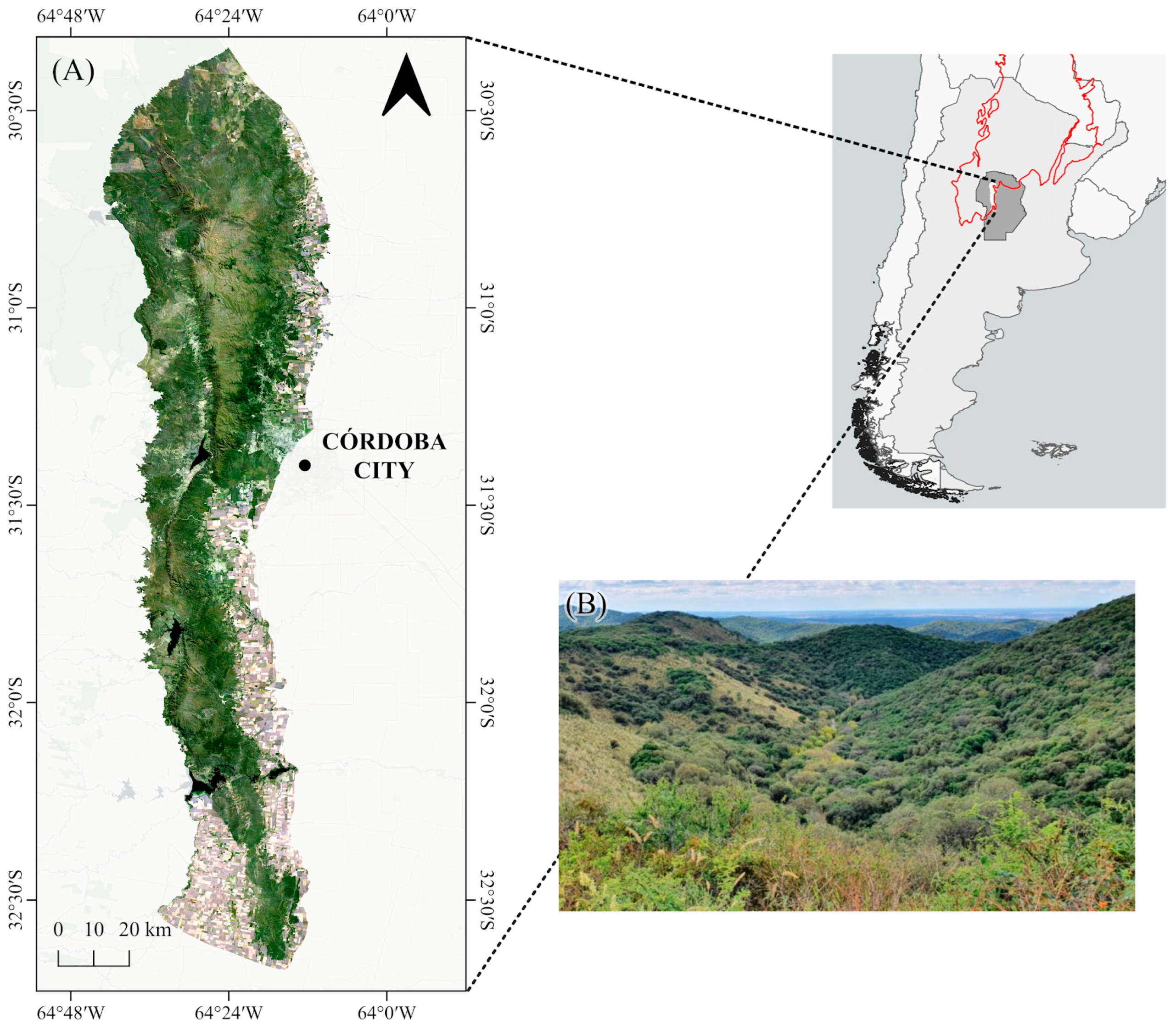
2.1. Study Area

The Sierras Chicas of Córdoba, in central Argentina, are located in the southern portion of the Gran Chaco (within the dry Chaco), stretching 250 km in a north–south direction, with an altitudinal range of 400 to 1900 m.a.s.l. and an area of 8400 km2 (Figure 1A). Vegetation is distributed in altitudinal belts [56], with Serrano forests (between 600 and 1300 m.a.s.l.) dominated by Schinopsis marginata, Zanthoxylum coco, Condalia buxifolia, Vachelia caven, Senegalia gillesii, Lithraea molleoides, Celtis ehrenbergiana, and Croton lachnostachys. Shrubs and early successional forests occur in a transition belt between 1300 and 1700 m.a.s.l., while grasses become dominant as elevation increases above 1500 m.a.s.l. (Figure 1B) [55,57,58]. A long history of LULC change has significantly altered the natural vegetation communities of the Sierras Chicas. Urban expansion, the invasion of exotic woody species (Ligustrum lucidum and Pinus sp.), wildfires, livestock grazing, and agriculture have been the primary drivers of these changes [52,53,59]. Collectively, these processes have exerted a profound negative impact on biodiversity, particularly on bird communities [60,61].

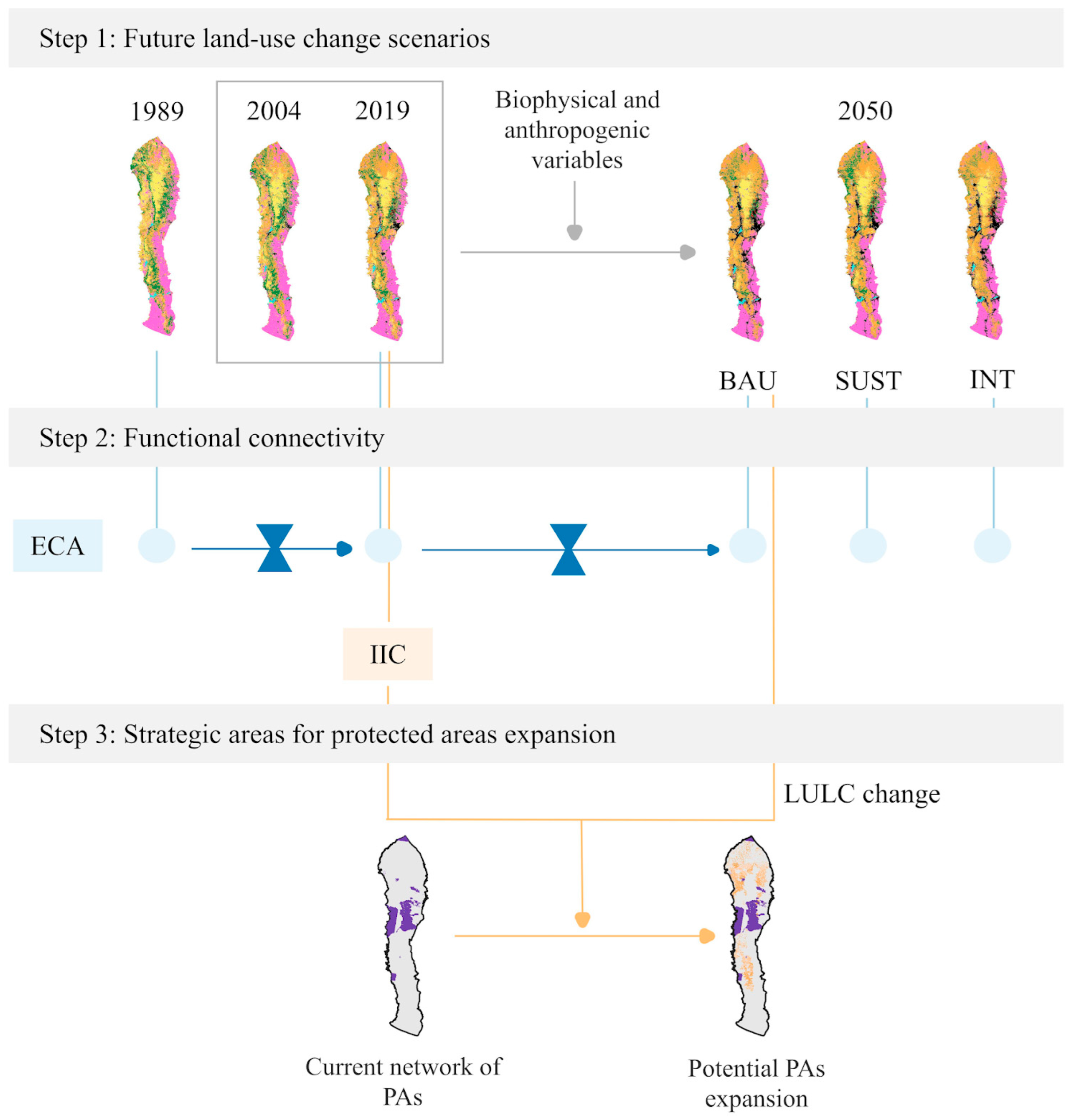
2.2. Future Land-Use Change Scenarios

Three spatially explicit LULC scenarios were modeled for 2050, based on a literature review and two workshops conducted with experts on LULC change in the study area (Figure 2). The 2050 horizon assessed longer-term effects, enabling the analysis of LULC change patterns and their potential ecological impacts [28].
Scenario 1. Business as usual (BAU). This scenario assumes that current LULC change trends will continue unchanged through the projected time horizon. Specifically, it assumes the following: (1) deforestation rates will persist at current levels, with no new restrictions, and even PAs may experience clearing events (as has occurred previously); [62]; (2) urban areas will continue to expand at current rates without spatial planning; and (3) invasive exotic tree species will continue to spread, further displacing native forests.
Scenario 2. Sustainability (SUST). This scenario envisions a more sustainable relationship between human activities and ecosystem conservation. It assumes the following: (1) all environmental regulations and deforestation-reduction policies are fully implemented and strictly enforced; (2) PAs effectively preserve native forests, preventing their loss and conversion to other land covers; (3) strict urban planning regulations are in place, with urban growth restricted to designated development zones [63]; (4) the expansion of the invasive species Ligustrum lucidum is controlled within PAs, and its use as an ornamental plant is prohibited; and (5) a reduction in the frequency of human-started wildfires.
Scenario 3. Intensification (INT). This scenario projects an intensification of the region’s current environmental challenges. It assumes the following: (1) an accelerated rate of urban expansion; (2) an increased rate of Ligustrum lucidum spread, surpassing that observed between 2004 and 2019 and resembling expansion rates from 1989 to 2004, along with the emergence of new invasion foci; (3) accelerated agricultural frontier expansion; and (4) increased wildfire frequency.
The spatial modeling of these scenarios was conducted using Dinamica EGO V5 software [64], which generates spatially explicit simulations based on historical land-use data. Land-cover maps from the 2004–2019 period were used (Figure 2) [52], as this timeframe reflects a recent and relatively stable period with regard to LULC dynamics. Land-cover maps include ten LULC classes: water, rock-bare soil, urban, productive land, grasslands, shrublands, native forest, glossy privet forest, pine forest, and acacia forest (further details on the land-cover maps development process, the LULC classes, and the accuracy assessment are provided in [52]). A set of biophysical and anthropogenic variables influencing LULC change in the area was selected for the model (Figure 2Appendix A). Dynamica EGO analyzes the relationship between historical land-cover changes (from 2004 to 2019) and the physical-environmental and anthropogenic variables used, in order to develop future projections. Once the model is trained, a projection for 2019 was generated using the 2004 land-cover map as input. To validate the model, we compared the simulated 2019 map with the observed land-cover map from 2019 using the “multi-resolution fit” metric implemented in Dinamica EGO [64]. This metric assesses spatial similarity by comparing patterns of land-use change within a moving window (in this case, 5 × 5 pixels) and returns a similarity index ranging from 0 (no match) to 1 (perfect match). Our validation resulted in a similarity index of 0.505, which meets the minimum threshold suggested by the software’s authors for acceptable model performance. Additional information regarding the scenario modeling can be found in [65] and in Appendix A.

2.3. Bird Species

A group of five native bird species was selected to represent a range of ecological profiles, including habitat preferences and varying sensitivities to land-use change (Table 1). The selection focused on species with distinct functional roles and contrasting habitat requirements within the ecosystem. Additionally, we included species with different conservation statuses and territorial behaviors to assess their potential responses under future land-use scenarios. This approach allows us to explore how diverse functional traits influence species’ vulnerability to landscape change and ensures representation of the broad diversity of bird species found in the Sierras.

2.4. Functional Connectivity

To assess changes in functional connectivity over the study period, we used the Equivalent Connected Area index (ECA) [70]. The ECA is a network-based metric that quantifies habitat availability and is particularly effective for monitoring variations in functional landscape connectivity [70]. The ECA is measured in area units, which allows for a direct comparison between changes in habitat connectivity and changes in total habitat area. It is defined as the size of a hypothetical, single, continuous habitat patch that would provide the same amount of reachable habitat as the actual configuration of habitat patches and connecting elements in the landscape under study [70,71].
To evaluate the contribution of individual patches to overall landscape connectivity, we used the Integral Index of Connectivity (IIC). The IIC is sensitive to both habitat availability and the spatial arrangement of habitat patches, and it allows for the identification of landscape elements that are most critical for maintaining connectivity (dIIC) [18,72].
ECA and IIC consider both the area and the habitat suitability of each habitat patch, as well as the distances between patches. Habitat suitability was determined based on a literature review for each species [61,66,67,68,69], assigning a value between 0 and 1 depending on the land-cover type (Table 2). Species-specific distance thresholds were defined using published data and field expertise to determine whether two patches should be considered connected (Table 2).
ECA was calculated for each species for three time points: the past (1989), the present (2019), and under three future scenarios (BAU, SUST, and INT) projected for the year 2050 (Figure 2). The relative change in ECA values (dECA, Equation (1)) was computed for two time intervals (1989–2019 and 2019–2050) and across the three scenarios.
dECA = ((ECA2 − ECA1)/ECA1) × 100,
where ECA1 is the ECA value before the change, and ECA2 is the ECA value after the change.
These dECA values were then compared to the relative change in habitat area (dA, Equation (2)).
dA = ((A2 − A1)/A1) × 100,
where A1 is the habitat area before the change, and A2 is the habitat area after the change.
This comparison between dECA and dA enables the assessment of whether changes in habitat area lead to disproportionately higher or lower variations in landscape connectivity [70]. dIIC was calculated for each species for the present (2019) (Figure 2). These calculations considered only areas occupied by grasslands, shrublands, and native forests, and included only patches larger than 4 hectares, due to data processing limitations. Both ECA and dIIC were calculated using the Makhurini package in R [73].

2.5. Strategic Areas for Protected Area Expansion

To identify potential strategic areas for expanding the PAs network while accounting for future changes and the functional connectivity of key bird species, we conducted a spatial prioritization using Zonation 5.0 software (Figure 2) [31,74]. Zonation is a decision-support tool for spatial planning and conservation [31,75]. It integrates spatial data on biodiversity features, such as species distributions or habitat types, along with information on anthropogenic pressures and existing PAs networks, generating a prioritization map that highlights areas based on their importance for biodiversity conservation [31].
We applied the CAZ2 cell-removal rule, which emphasizes areas with high average biodiversity value, while also improving the representation of underrepresented features, those whose distribution does not overlap significantly with other biodiversity attributes, even if this slightly reduces the overall coverage of areas with high average richness [74].
The prioritization focused on areas occupied by grasslands, shrublands, and native forests. The biodiversity features used in the analysis consisted of the five studied bird species, with each species represented by its dIIC values previously calculated for each habitat patch. Higher priority was assigned to those areas within each land-cover type with probability of habitat loss by 2050, based on the BAU scenario (Figure 2). This approach allowed us to simultaneously account for the following: (i) habitat availability for each species, (ii) the importance of each patch for maintaining landscape functional connectivity for each species, and (iii) the risk of patch loss by 2050. A hierarchical mask of the existing PAs network in the Sierras Chicas was included (Appendix B), allowing us to achieve the following: (1) evaluate the effectiveness of the current PAs network in representing the studied species, and (2) identify priority areas, within the top 17% and 30% of the landscape, as aligned with the Aichi Biodiversity Targets and the post-2020 Global Biodiversity Framework [13,14] that are not currently under protection, as potential sites for PAs network expansion.

3. Results

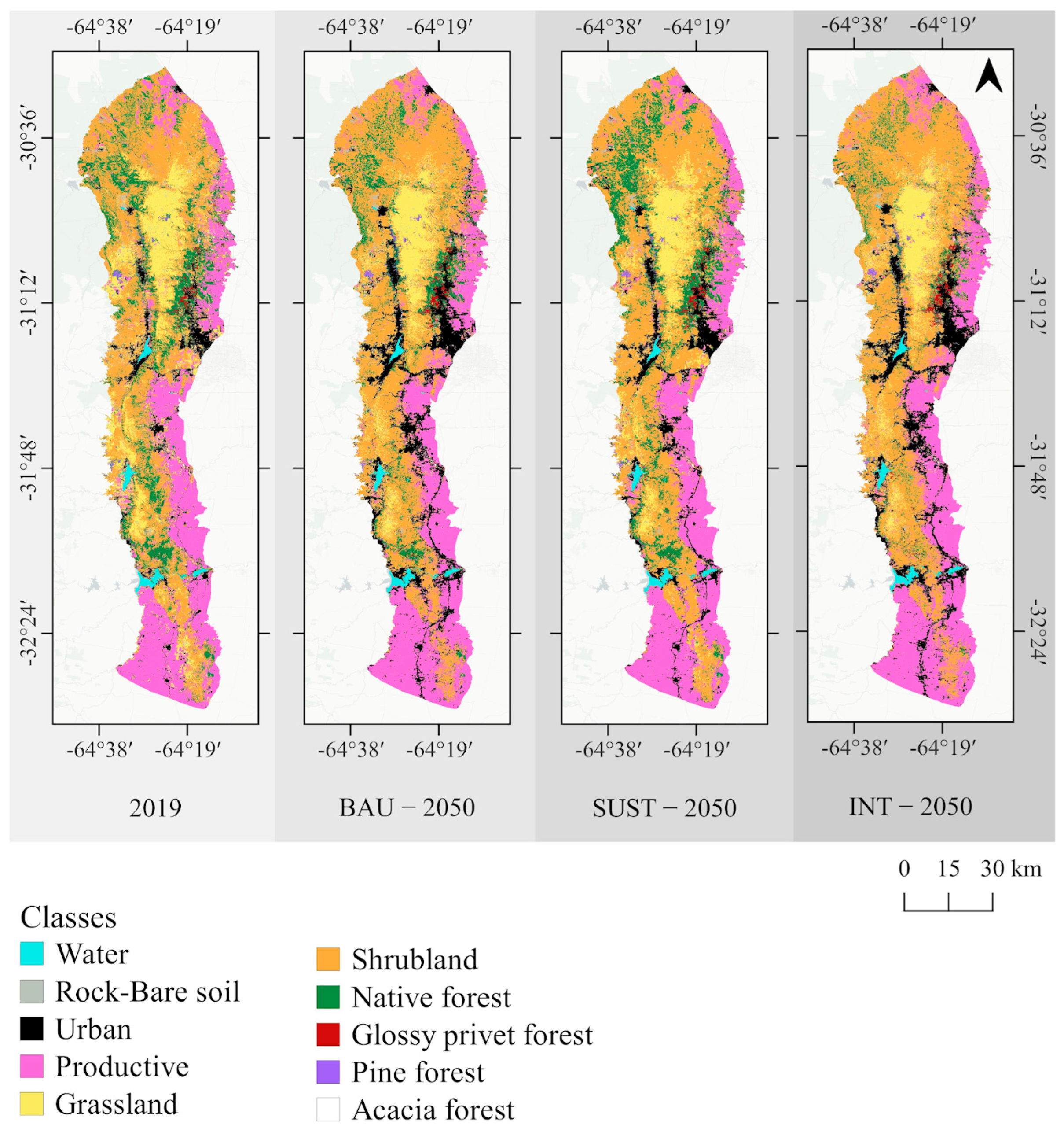
3.1. Future Land-Use Change Scenarios

The three scenarios were generated and spatialized for 2050 (Figure 3). During the model validation process, a match of 50% (0.505) was achieved between the real and simulated maps using a 5 × 5 pixel window.
Grasslands would decline in all three scenarios. This reduction would be similar in both the BAU and INT scenarios, and slightly lower in the SUST scenario (Figure 3/Appendix C). In all scenarios, the loss of grasslands would be largely compensated for by an increase in shrublands, with smaller portions converted to productive or urban land. Shrublands would expand in all scenarios, with the most pronounced increase occurring under the INT scenario (Figure 3/Appendix C).
Native forests would undergo a substantial reduction in all scenarios. Between 2019 and 2050, the BAU scenario would result in a loss of 64,000 hectares of native forest (59% of the 2019 native forests extent). The SUST scenario would see a smaller loss of approximately 45,000 hectares (42%), while the INT scenario would lead to a loss of 81,000 hectares (74%) (Figure 3/Appendix C).
All three scenarios showed a significant increase in urban areas. In the BAU scenario, urban expansion is projected to reach 62,000 hectares between 2019 and 2050. In contrast, the SUST scenario anticipates a more moderate increase, with growth occurring in a more compact form and restricted to areas specifically designated for urban development. The INT scenario projects the greatest expansion in urban areas among the three scenarios (Figure 3/Appendix C). Productive land would show relatively little variation in extent across the three scenarios. In both the BAU and SUST scenarios, a decrease in productive areas is expected, whereas the INT scenario would result in a slight increase (Figure 3/Appendix C).

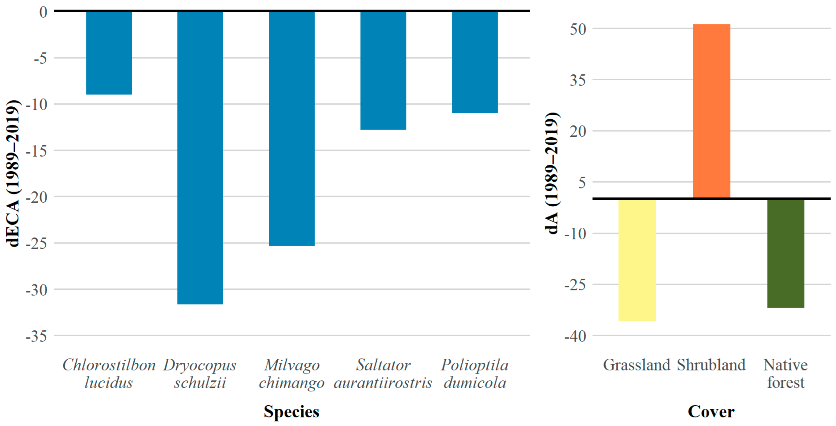
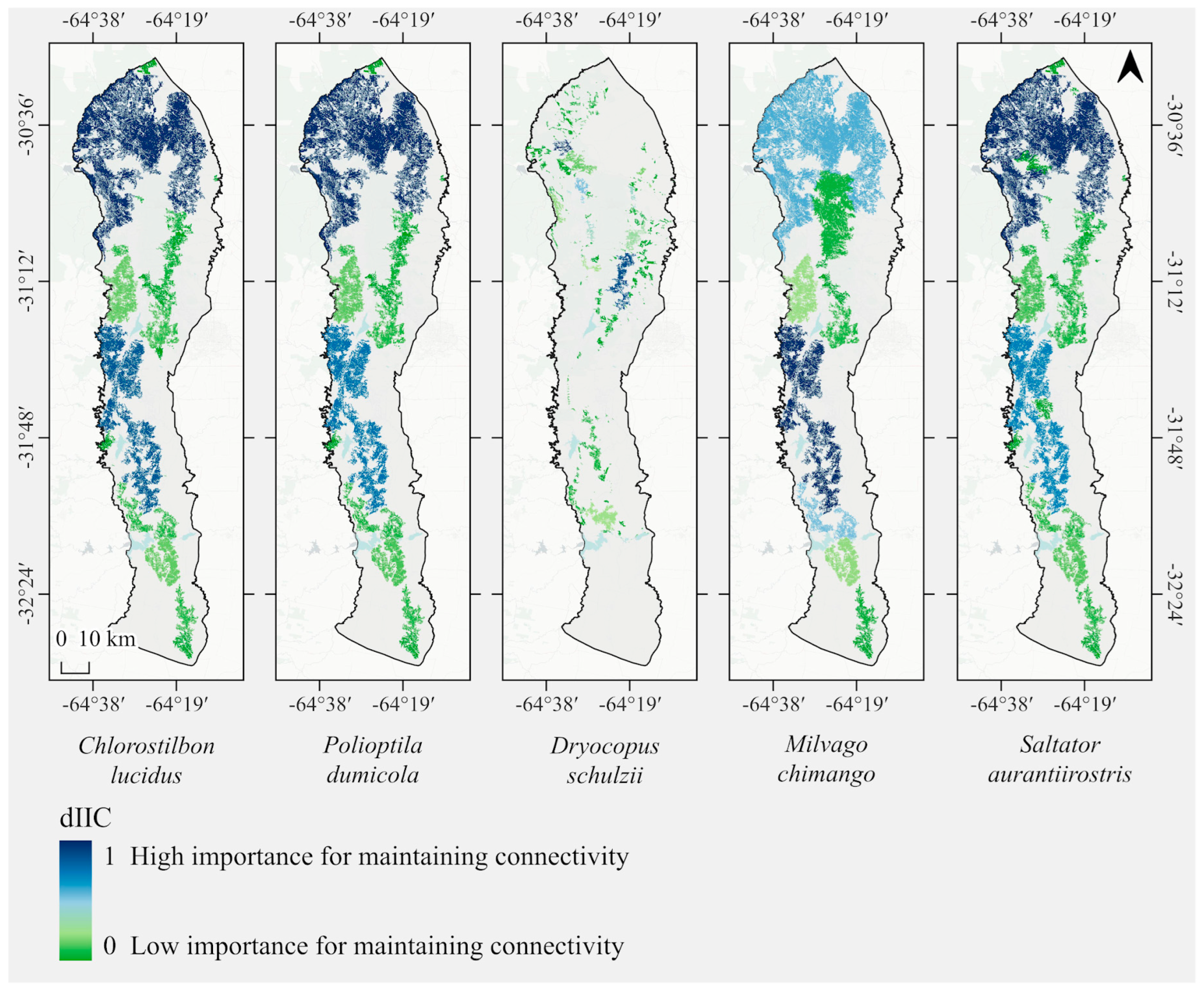
3.2. Functional Connectivity

Functional connectivity varied among the five species, across the three time points, and under the three modeled scenarios. All five species experienced a decline in functional connectivity between 1989 and 2019, with Dryocopus schulzii exhibiting the greatest loss (−34%) and Polioptila dumicola the smallest (−7%) (Figure 4). For Dryocopus schulzii, the relative change in equivalent connected area was similar to the relative change in native forest area (dECA ≅ dA). In Milvago chimango, dECA < dA for grasslands. In Chlorostilbon lucidus, Polioptila dumicola, and Saltator aurantiirostris, dECA values were negative, despite positive dA values for shrublands and negative dA values for native forests and grasslands (Figure 4/Appendix D).
Between 2019 and 2050, most species are projected to continue losing functional connectivity under all three scenarios (Figure 5). For all five species, the greatest losses are expected under the SUST scenario. Dryocopus schulzii is projected to remain the most affected species, experiencing the highest connectivity losses. In contrast, Polioptila dumicola is expected to show a slight gain in functional connectivity under the BAU and INT scenarios (Figure 5). Over this period, the relative change in habitat area (dA) is projected to remain negative for native forests and grasslands and positive for shrublands across all scenarios (Figure 5).
The dIIC values for each habitat patch varied among the studied species. While some species, like Chlorostilbon lucidus, Polioptila dumicola, and Saltator aurantiirostris shared a similar pattern of high-importance patches for maintaining landscape functional connectivity, others species like Dryocopus schulzii and Milvago chimango exhibited distinct patterns, with different sets of patches contributing most significantly to functional connectivity (Figure 6).

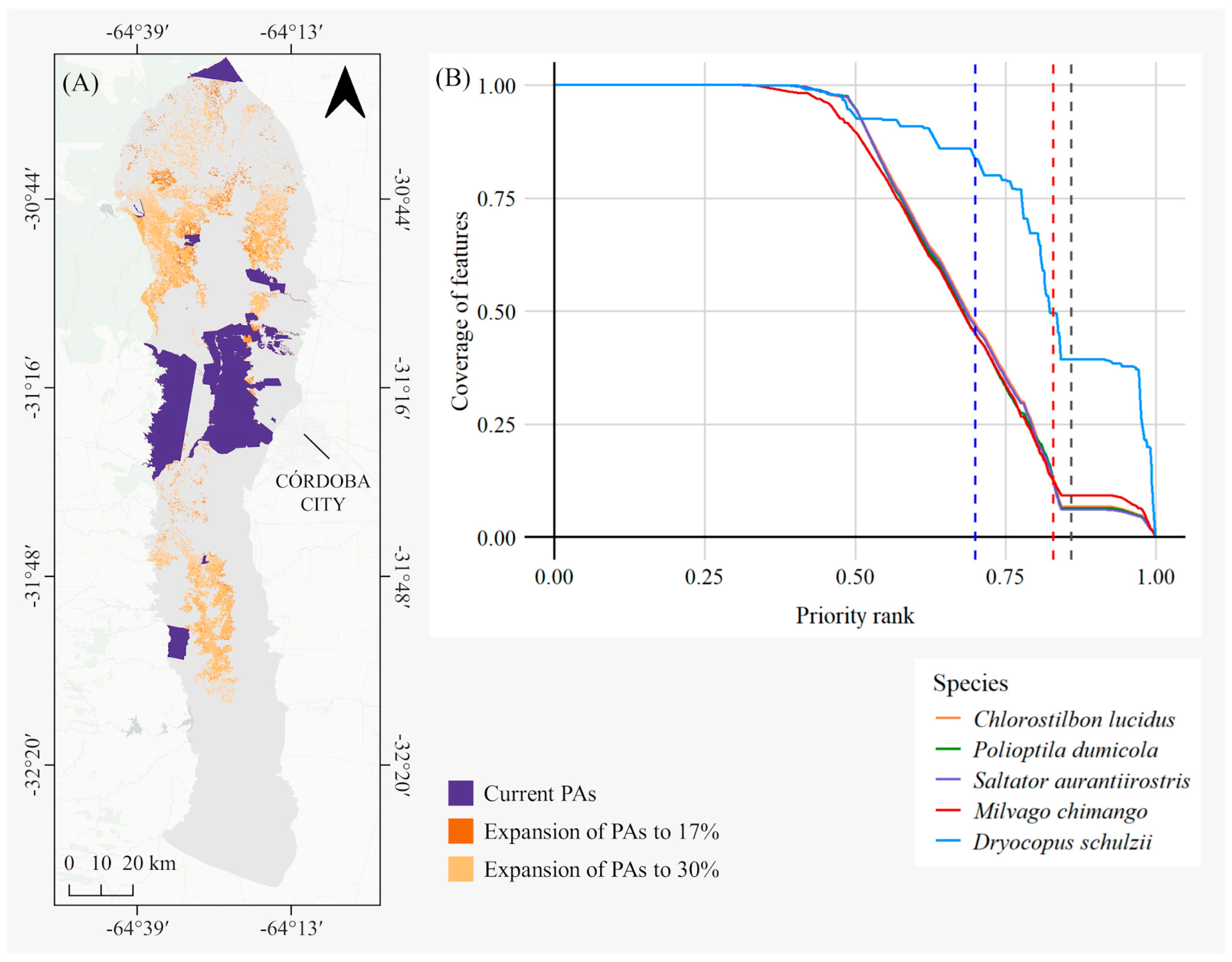
3.3. Strategic Areas for Protected Area Expansion

Based on the existing network of PAs within the study region, pixels with high priority values were identified as potential sites for PAs network expansion, aiming to achieve 17% (color: dark orange) and 30% (color: dark orange + light orange) coverage of the study area’s surface (Figure 7A). Although the high-priority pixels are spatially dispersed, several zones with a notable concentration of such pixels, herein referred to as high-priority patches, can be identified.
The performance curves illustrate the effectiveness of the spatial prioritization in capturing the habitat of each target species (Figure 7B). Among the species analyzed, Dryocopus schulzii exhibited the highest level of representation under the current prioritization. In contrast, the remaining species displayed lower, but relatively similar, levels of representation. Currently, the existing PAs system, which covers 14% of the study area (black dashed line), includes 39% of Dryocopus schulzii’s habitat and only 6–9% of the habitat of the other species. If the network were expanded to cover 17% of the region (red dashed line), the representation of Dryocopus schulzii’s habitat would increase to 49%, and that of the other species to approximately 12%. Further expansion to 30% (blue dashed line) would increase the representation of Dryocopus schulzii’s habitat to 84%, while the other species would reach representation levels between 45% and 47% (Figure 7B).

4. Discussion

The methodology employed enabled the projection of future LULC changes in the Sierras Chicas, as well as the assessment of past, present, and future functional connectivity for the bird species analyzed. The results allowed the identification of key landscape patches with high ecological relevance for maintaining the connectivity of the target species, which are also at high risk of future loss. These areas are proposed as priorities for the expansion of the PAs network or the implementation of complementary conservation strategies. This approach integrates LULC change dynamics with the habitat requirements of local indicator species, facilitating the identification of priority conservation zones. The methodology is transferable and can be applied in other regions where landscape transformation threatens ecological connectivity, allowing for proactive and precise conservation planning.
Systematic conservation planning often focuses on preserving either species’ distribution ranges or landscape connectivity, but rarely addresses both simultaneously [76]. In the Sierras Chicas, the results of functional connectivity assessments under the different future scenarios highlight the importance of incorporating functional connectivity as a central component of conservation planning. As observed in other regions [77], the studied species exhibited different responses to historical and projected LULC changes, with connectivity patterns that did not always match expectations. This was particularly evident in the sustainability scenario, which (contrary to what we expected) resulted in the greatest decline in functional connectivity for all species among the three scenarios analyzed. This finding emphasizes the need for conservation planning approaches that go beyond habitat availability alone and consider how landscape spatial configuration affects connectivity between habitat patches, ultimately influencing species persistence in the face of land-use change and climate change [78,79].
Between 1989 and 2019, all species experienced a decline in their functional connectivity. This is consistent with the trend of declining functional connectivity observed in other regions and species in recent years [77,80,81]. Dryocopus schulzii and Milvago chimango, both species highly dependent on native forests and grasslands which were the most impacted land-cover types, were the most affected. In Dryocopus schulzii, a species closely associated with forests, the relative variation in available habitat area was similar to the variation in equivalent connected area, indicating that the loss of connectivity was proportional to habitat loss [70]. In contrast, for Milvago chimango (a generalist species, though primarily associated with grasslands) the relative habitat loss was greater than the relative decrease in connectivity, suggesting greater resilience in terms of functional connectivity [70,81]. In the case of Chlorostilbon lucidus, Polioptila dumicola, and Saltator aurantiirostris, species primarily associated with shrublands but also using forests and grasslands, delta equivalent connected area values were lower but consistently negative. This suggests that, despite the increase in shrubland cover during the study period, the loss and fragmentation of native forests and grasslands negatively affected their functional connectivity. These findings reinforce the importance of adopting an integrated landscape perspective in conservation efforts, rather than focusing actions in isolation on individual land-cover types [82,83].
The projected scenarios help identify areas with a high probability of change, particularly the loss of habitat patches [84]. In the Sierras Chicas, there has been a consistent trend of deforestation and LULC change since the 1970 s, seriously threatening the persistence of native forests and grasslands [52,53,62], and current management and conservation policies are insufficient to ensure their long-term sustainability. The three analyzed scenarios consistently projected continued loss of native vegetation cover. In both the business as usual and intensification scenarios, forest and grassland loss continues at a high rate. In the sustainability scenario, forest loss slowed down, but grassland loss remains high. This suggests that reversing the degradation of the Serrano ecosystem will require more ambitious and diversified policies.
Contrary to expectations, by 2050, the greatest losses in functional connectivity are projected under the sustainability scenario. This indicates that although this scenario may reduce the rate of native cover loss, it does not necessarily ensure the functional connectivity of the species. In fact, the distribution of conserved patches tends to be more isolated, reducing their functional value for species movement. This highlights that preserving habitat area alone is not sufficient to maintain connectivity, especially when newly conserved or restored areas are not strategically located. As observed during the historical period (1989–2019), Dryocopus schulzii remains the most affected species (in all scenarios), reflecting its strong dependence on native forest, projected to be the most heavily lost land-cover type in the region. The variability in species responses across scenarios highlights the complexity of the relationship between LULC and functional connectivity, particularly for species that use multiple habitat types with varying suitability [77,85,86]. Although the sustainability scenario scope was on natural-vegetation cover conservation in the face of anthropogenic pressures, it did not explicitly address functional connectivity, emphasizing the need to incorporate this aspect into future planning. Likewise, the high interspecific variability observed reinforces the importance of adopting conservation approaches based on a suite of indicator species [87]. Using a diverse set of species captures a broader range of ecological responses and facilitates the identification of key conservation areas that benefit a larger number of species [88].
Currently, the existing PAs network covers only a small proportion of the habitat of Milvago chimango, Polioptila dumicola, Saltator aurantiirostris, and Chlorostilbon lucidus, leaving critical areas unprotected and vulnerable to landscape transformation. Many of these priority areas lie outside the formal PAs system and face a high probability of loss in the short to medium term. This situation is further compounded by the fact that most PAs in Córdoba exist only “on paper”, that is, they do not meet basic implementation standards [89]. Together, these factors highlight the high conservation risk faced by these species in the Sierras Chicas, a region with a long history of LULC change [52,53,62].
Although a complete redesign of the PAs system is unfeasible, its strategic expansion based on spatial prioritization can significantly enhance its effectiveness [90]. Currently, only 14% of the Sierras Chicas is under some form of protection, well below international targets such as the Aichi Biodiversity Targets and the Post-2020 Global Biodiversity Framework [13,14]. Expanding the network to cover 30% of the territory would significantly improve the representativeness of the studied species, with a relatively moderate investment.
In addition to expanding the PAs network and building on the previously mentioned concept of the importance of planning conservation from an integrated landscape perspective, it is essential to improve the quality of the surrounding matrix, which acts as a buffer zone and facilitates ecological connectivity [82,91,92,93]. The identification of corridors or wildlife passages that connect patches of natural vegetation can build upon the prioritization analyses developed in this study. In this context, the IIC is a valuable tool for assessing the potential contribution of new patches to landscape connectivity and informing restoration actions [18].
Since each species has different distributions and ecological requirements, the habitat patches that are critical for maintaining landscape connectivity varied among the species analyzed [94]. Therefore, the spatial prioritization carried out in this study reflects the specific needs of this particular group of species. Designing an integrated and complementary PAs network requires incorporating representative information from a diverse set of species, thereby strengthening the network’s resilience and conservation effectiveness [90,95,96].
The proposed expansion of the protected area network must be understood within the context of ongoing and intensifying land-use pressures, particularly urbanization and agricultural expansion, which are dominant drivers of habitat loss and fragmentation in the Sierras Chicas. These pressures can undermine the long-term effectiveness of protected areas by isolating habitat patches and degrading the surrounding matrix, thereby reducing functional connectivity. Consequently, conservation planning should not only prioritize the identification and protection of key habitat patches but also incorporate land-use management strategies that address agricultural practices and urban development. Integrating connectivity-based spatial prioritization with land-use zoning, sustainable agriculture, and urban planning policies will be critical to mitigate negative impacts and ensure the persistence of biodiversity in this rapidly changing landscape. Furthermore, enhancing ecological corridors and buffer zones around protected areas can facilitate species movement and resilience to land-use pressures.

5. Conclusions

Conservation efforts often focus on protecting habitat for flagship species, while rarely accounting for their connectivity needs [76,97]. It is essential to include connectivity as a key indicator in conservation planning, using a broad set of indicator species to capture diverse habitat requirements [15,78,79,88]. Although the lack of data on species movement and ecological needs poses limitations [16], the methodology proposed here allows for the generation of useful insights using accessible data, and it can be refined as more information becomes available. On the other hand, scenario modeling and the use of indices such as the IIC provide a means to test different alternatives according to future potential risks, anticipate species responses to environmental change, and guide restoration actions with greater confidence in their positive effects on functional connectivity [18,28]. In our case, the unexpectedly lower connectivity loss under the BAU scenario may result from the persistence of large forest patches in areas less affected by land-use pressures, which act as key structural elements in the landscape. In contrast, the sustainability scenario, despite promoting vegetation recovery, may lead to more fragmented configurations if restoration occurs in isolated or suboptimal areas. These findings underscore the importance of integrating spatial configuration—not just habitat extent—into conservation strategies.
In the current context of the Sierras Chicas, characterized by strong LULC change trends, a lack of spatial planning and weak governmental regulation means that the business-as-usual scenario appears likely to materialize [52,53,62], with significant consequences for biodiversity connectivity. In light of this situation, broader measures are required that not only preserve existing fragments but also promote the restoration of degraded areas and support the regeneration of natural cover and species connectivity.

Author Contributions

J.R.A., writing of the original draft, data collection, and formal analysis. L.E.S., preparation and validation of future scenarios, support for species selection and characterization, writing—review and editing. L.M.B. and G.G.P., conceptualization, writing—review and editing. C.B., M.P.A., M.C.N.-F. and J.V.A. writing—review and editing. All authors have read and agreed to the published version of the manuscript.

Funding

This research was funded by CONICET (PIP-2021 #11220200101287), FONCyT (PICT-2020 #1329) and PID, CONSOLIDAR SECYT UNC.

Institutional Review Board Statement

Not applicable.

Informed Consent Statement

Not applicable.

Data Availability Statement

Data are contained within the article or Appendixes. Dataset available on request from the authors.

Acknowledgments

We are very grateful to P. Huais for the mathematical support provided in the development of the scenarios. This research was supported by CONICET (PIP-2021 #11220200101287), FONCyT (PICT-2020 #1329) and PID, CONSOLIDAR SECYT UNC. This study is part of the research of J.R.A. as a doctoral fellow at CONICET. G.G.P. is a researcher at CONICET and INTA. L.E.S. has a fellowship at CONICET. L.M.B. is a researcher at CONICET and a professor at the Facultad de Ciencias Exactas, Físicas y Naturales, Universidad Nacional de Córdoba (UNC). C.B. is a researcher at CONICET. M.P.A. and M.C.N.F. have a doctoral fellowship at CONICET. J.V.A. is a student at Instituto Gulich. We are thankful for the financial support, only possible with sustainable public policies for science.

Conflicts of Interest

The authors declare no conflicts of interest. The funders had no role in the design of the study; in the collection, analyses, or interpretation of data; in the writing of the manuscript; or in the decision to publish the results.

Abbreviations

The following abbreviations are used in this manuscript:
LULCLand-Use/Land-Cover
PAsProtected areas
BAUBusiness-as-usual scenario
SUSTSustainability scenario
INTIntensification scenario
IUCNInternational Union for Conservation of Nature
ECAEquivalent Connected Area index
IICIntegral Index of Connectivity
dECARelative change in equivalent connected area
dARelative change in habitat area

Appendix A. Future Land-Use Change Scenario Modeling

Because the dynamics of LULC change vary within the study area, the area was divided into three subregions for scenario modeling:
  • Urban Zone: a 300 m buffer surrounding the main urban areas. This distance was chosen because it approximates the extent of urban expansion between 2004 and 2019.
  • Non-Urban Zone: the area outside the main urban settlements and their buffer zones.
  • Northwest Zone: a native forest area located in the northern part of the study area, away from extensive urbanization and invasions of exotic tree species.
For scenario development, LULC maps from 2004 and 2019 were used, along with a set of physical-environmental and anthropogenic variables (Table A1). The land-cover maps employed correspond to those produced by [52]. These maps include ten LULC classes: water, rock-bare soil, urban, productive land, grasslands, shrublands, native forest, glossy privet forest, pine forest, and acacia forest. Further details on the map development process, the classified LULC categories, and the accuracy assessment are provided in [52].
Table A1. Physical-environmental and anthropogenic variables used for scenario modeling.
VariableDescriptionSource
Physical-environmental
Altitude (m.a.s.l.) DEM NASA SRTM version 3.0 [98]
Slope (degrees) Derived from the digital elevation model
Orientation (degrees)
Temperature (°C)Mean value for the period 1940–2000WorldClim BIO12 [99]
Annual precipitation (mm)
AridityMartonne aridity indexAtlas Climático digital de la República Argentina [100]
Distance to water (m)Distance to watercourse or waterbodyAdministración Provincial de Recursos Hídricos
Native forest patch area (ha)The pixel value represents the area of the native forest patch it is part of[52]
Distance to grassland (m)Distance from each raster pixel to the corresponding class, cover type, or feature of interest[52]
Distance to shrubland (m)
Distance to native forest (m)
Distance to glossy privet forest (m)
Distance to pine forest (m)
Antropic
Fire frecuencyFire frecuency between 2004 and 2018[101]
Population density (Hab/km2)Population density derived from the 2001 and 2010 national census data[102]
Distance to roads (m)Distance to primary, secondary, and tertiary roadsMapas Córdoba–IDECOR
Distance to urban areas (m)Distance from each raster pixel to the corresponding class, cover type, or feature of interest[52]
Distance to productive areas (m)
The magnitude and direction of LULC changes between 2004 and 2019 were quantified using Markov transition matrices, which indicate the proportion of a given land-cover type at time T1 that transitions to another type at time T2. The following transitions were modeled:
Productive >> Urban
Productive >> Shrubland
Grassland >> Urban
Grassland >> Productive
Grassland >> Shrubland
Grassland >> Native Forest
Shrubland >> Urban
Shrubland >> Productive
Shrubland >> Native Forest
Native Forest >> Urban
Native Forest >> Productive
Native Forest >> Grassland
Native Forest >> Shrubland
Native Forest >> Glossy privet Forest
Native Forest >> Pine Forest
Glossy privet Forest >> Urban
Dynamica EGO analyzes the relationship between historical land-cover changes (from 2004 to 2019) and the physical-environmental and anthropogenic variables used, in order to develop future projections. Once the model is trained, a projection is generated using the 2004 land-cover map, and the simulated 2019 map is validated by comparing it to the actual 2019 map using a similarity metric. Finally, a 3 × 3 pixel majority filter was applied to the simulated maps to reduce noise and eliminate spurious pixels. One limitation of the model is its reliance on LULC maps, which contain inherent uncertainties that may be propagated or even amplified during the simulation process. Additionally, LULC transition rates are assumed to remain constant over the entire study period, which may not adequately capture the temporal dynamics of actual land-cover and land-use changes [103]. Addressing this limitation would require dividing the simulation period into distinct temporal stages. Both aspects underscore the importance of having prior knowledge of the study area to inform appropriate modeling decisions.
Additional information regarding the scenario modeling can be found in [65].

Appendix B

Table A2. Protected Area Network of the Sierras Chicas.
Name
National PAsLa Calera
Ascochinga
Provincial PAsReserva forestal natural Uritorco
Reserva forestal natural Sierras de Punilla
Reserva hídrica natural los Gigantes
Reserva hídrica natural la Quebrada
Corredor biogeográfico Chaco Árido
Municipal PAsÁrea protegidas AP1 Villa Carlos Paz
Reserva urbana San Martín
Reserva natural Quisquisacate
Reserva forestal natural Sierra de Cuniputo
Reserva hídrica natural Salsipuedes
Reserva de uso múltiple Villa General Belgrano
Reserva hídrica natural Villa Cerro Azul
Reserva natural de uso múltiple de la Rancherita
Reserva natural municipal el Portecelo
Reserva ecológica recreativa Cuesta Blanca
Reserva natural cultural recreativa municipal Tanti
Reserva parque recreativo natural Río Yuspe
Reserva natural comunal Camin Cosquín
Reserva hídrica recreativa natural Saldán Inchin
Reserva hídrica recreativa natural Bamba
Área natural protegidas Villa Cielo
Reserva los Manantiales
Reserva hídrica recreativa Villa Allende
Reserva hídrica recreativa los Quebrachitos
Reserva Tiu Mayu
Reserva hídrica recreativa natural Mendiolaza
Área de protección Alta Gracia

Appendix C

Table A3. Area (ha) of different land-cover types in the Sierras Chicas of Córdoba for the year 2019 and for the 2050 scenarios: BAU, SUST, and INT.
20192050
BAUSUSTINT
Urban50 822.72109 688.3973 307.73111 754.18
Productive215 900.50206 441.30205 228.32216 827.65
Grassland114 156.3875 161.1181 138.6974 826.44
Shrubland323 393.63350 368.13351 369.91362 057.75
Native forest108 200.5370 764.31101 543.9645 774.14
Glossy privet forest4 147.114 981.214 916.266 318.85
Pine forest2 393.913 124.802 980.502 997.23

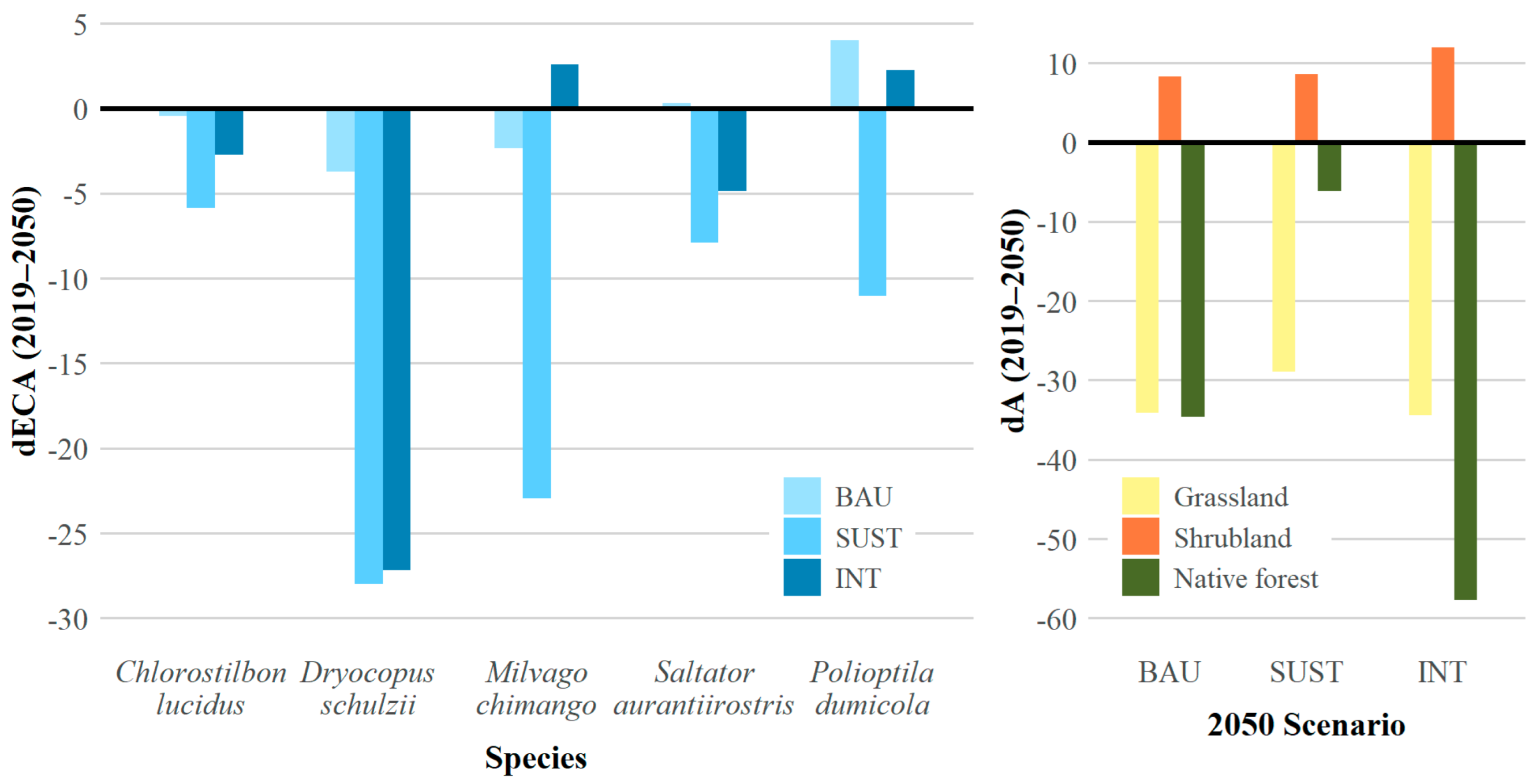
Appendix D. dECA and dA Values

Table A4. dECA values for 1989–2019 and for 2019–2050.
1989–20192019–2050
BAUSUSTINT
Chlorostilbon lucidus−15.19−0.43−5.85−2.71
Dryocopus schulzii−33.83−3.71−27.97−27.18
Milvago chimango−26.93−2.36−22.972.58
Saltator aurantiirostris−14.540.31−7.92−4.87
Polioptila dumicola−7.364.00−11.012.25
Table A5. dA values for 1989–2019 and for 2019–2050.
1989–20192019–2050
BAUSUSTINT
Grassland−35.82−34.16−28.92−34.45
Shrubland51.158.348.6511.96
Native forest−31.93−34.60−6.15−57.70

References

  1. Smith, P.; House, J.I.; Bustamante, M.; Sobocká, J.; Harper, R.; Pan, G.; West, P.C.; Clark, J.M.; Adhya, T.; Rumpel, C.; et al. Global Change Pressures on Soils from Land Use and Management. Glob. Change Biol. 2019, 22, 1008–1028. [Google Scholar] [CrossRef]
  2. Song, X.P.; Hansen, M.C.; Stehman, S.V.; Potapov, P.V.; Tyukavina, A.; Vermote, E.F.; Townshend, J.R. Global land change from 1982 to 2016. Nature 2018, 560, 639–643. [Google Scholar] [CrossRef]
  3. Winkler, K.; Fuchs, R.; Rounsevell, M.; Herold, M. Global land use changes are four times greater than previously estimated. Nat. Commun. 2021, 12, 2501. [Google Scholar] [CrossRef] [PubMed]
  4. Pimm, S.L.; Raven, P. Extinction by numbers. Nature 2000, 403, 843–845. [Google Scholar] [CrossRef]
  5. Davison, C.W.; Rahbek, C.; Morueta-Holme, N. Land-use change and biodiversity: Challenges for assembling evidence on the greatest threat to nature. Glob. Change Biol. 2021, 27, 5414–5429. [Google Scholar] [CrossRef] [PubMed]
  6. Jaureguiberry, P.; Titeux, N.; Wiemers, M.; Bowler, D.E.; Coscieme, L.; Golden, A.S.; Jacob, U. The direct drivers of recent global anthropogenic biodiversity loss. Sci. Adv. 2022, 8, eabm9982. [Google Scholar] [CrossRef] [PubMed]
  7. Chapin, F.S., III; Zavaleta, E.S.; Eviner, V.T.; Naylor, R.L.; Vitousek, P.M.; Reynolds, H.L.; Hooper, D.U.; Lavorel, S.; Sala, O.E.; Hobbie, S.E.; et al. Consequences of changing biodiversity. Nature 2000, 405, 234–242. [Google Scholar] [CrossRef]
  8. Faria, D.; Morante-Filho, J.C.; Baumgarten, J.; Bovendorp, R.S.; Cazetta, E.; Gaiotto, F.A.; Mariano-Neto, E.; Mielke, M.S.; Pessoa, M.S.; Rocha-Santos, L.; et al. The breakdown of ecosystem functionality driven by deforestation in a global biodiversity hotspot. Biol. Conserv. 2023, 283, 110126. [Google Scholar] [CrossRef]
  9. Taylor, B.M.; McIlwain, J.L.; Kerr, A.M. Marine reserves and reproductive biomass: A case study of a heavily targeted reef fish. PLoS ONE 2012, 7, e39599. [Google Scholar] [CrossRef]
  10. Ghosh-Harihar, M.; An, R.; Athreya, R.; Borthakur, U.; Chanchani, P.; Chetry, D.; Datta, A.; Harihar, A.; Karanth, K.K.; Mariyam, D.; et al. Protected areas and biodiversity conservation in India. Biol. Conserv. 2019, 237, 114–124. [Google Scholar] [CrossRef]
  11. Geldmann, J.; Manica, A.; Burgess, N.D.; Coad, L.; Balmford, A. A global-level assessment of the effectiveness of protected areas at resisting anthropogenic pressures. Proc. Natl. Acad. Sci. USA 2019, 116, 23209–23215. [Google Scholar] [CrossRef] [PubMed]
  12. Marcos, C.; Díaz, D.; Fietz, K.; Forcada, A.; Ford, A.; García-Charton, J.A.; Goñi, R.; Lenfant, P.; Mallo, S.; Mouillot, D.; et al. Reviewing the ecosystem services, societal goods, and benefits of marine protected areas. Front. Mar. Sci. 2021, 8, 613819. [Google Scholar] [CrossRef]
  13. Convention on Biological Diversity (CBD). Strategic Plan for Biodiversity 2011–2020 and the Aichi Targets. In Decisions Adopted by the Conference of the Parties to the Convention on Biological Diversity at Its Tenth Meeting; Secretariat of the Convention on Biological Diversity: Montreal, QC, Canada, 2010. [Google Scholar]
  14. Convention on Biological Diversity (CBD). Report of the Open-ended Working Group on the Post-2020 Global Biodiversity Framework on its third meeting. In Proceedings of the Open-Ended Working Group on the Post-2020 Global Biodiversity Framework. Third Meeting, Online, 23 August–3 September 2021. [Google Scholar]
  15. Rudnick, D.; Ryan, S.; Beier, P.; Cushman, S.A.; Dieffenbach, F.; Epps, C.W.; Gerber, L.; Hartter, J.; Jenness, J.S.; Kintsch, J.; et al. The role of landscape connectivity in planning and implementing conservation and restoration priorities. Issues Ecol. 2012, 16, 20. [Google Scholar]
  16. Keeley, A.T.; Beier, P.; Jenness, J.S. Connectivity metrics for conservation planning and monitoring. Biol. Conserv. 2021, 255, 109008. [Google Scholar] [CrossRef]
  17. Correa Ayram, C.A.; Mendoza, M.E.; Etter, A.; Salicrup, D.R.P. Habitat connectivity in biodiversity conservation: A review of recent studies and applications. Prog. Phys. Geogr. 2016, 40, 7–37. [Google Scholar] [CrossRef]
  18. Pascual-Hortal, L.; Saura, S. Comparison and development of new graph-based landscape connectivity indices: Towards the prioritization of habitat patches and corridors for conservation. Landsc. Ecol. 2006, 21, 959–967. [Google Scholar] [CrossRef]
  19. Brussaard, L.; Caron, P.; Campbell, B.; Lipper, L.; Mainka, S.; Rabbinge, R.; Babin, D.; Pulleman, M. Reconciling biodiversity conservation and food security: Scientific challenges for a new agriculture. Curr. Opin. Environ. Sustain. 2010, 2, 34–42. [Google Scholar] [CrossRef]
  20. Mosciaro, M.J.; Calamari, N.C.; Peri, P.L.; Montes, N.F.; Seghezzo, L.; Ortiz, E.; Rejalaga, L.; Barral, P.; Villarino, S.; Mastrangelo, M.; et al. Future scenarios of land use change in the Gran Chaco: How far is zero deforestation? Reg. Environ. Change 2022, 22, 115. [Google Scholar] [CrossRef]
  21. Malek, Z.; Boerboom, L.; Glade, T. Future forest cover change scenarios with implications for landslide risk: An example from Buzau Subcarpathians. Environ. Manag. 2015, 56, 1228–1243. [Google Scholar] [CrossRef]
  22. Tejada, G.; Dalla-Nora, E.; Cordoba, D.; Lafortezza, R.; Ovando, A.; Assis, T.; Aguiar, A.P. Deforestation scenarios for the Bolivian lowlands. Environ. Res. 2016, 144, 49–63. [Google Scholar] [CrossRef]
  23. IPBES. Summary for Policymakers of the Global Assessment Report on Biodiversity and Ecosystem Services of the Intergovernmental Science-Policy Platform on Biodiversity and Ecosystem Services; Zenodo: Geneva, Switzerland, 2019. [Google Scholar] [CrossRef]
  24. IPCC. Summary for policymakers. In Climate Change 2023: Synthesis Report; Contribution of Working Groups I, II and III to the Sixth Assessment Report of the Intergovernmental Panel on Climate Change; Core Writing Team, Lee, H., Romero, J., Eds.; IPCC: Geneva, Switzerland, 2023; pp. 1–34. [Google Scholar]
  25. Dockerty, T.; Lovett, A.; Appleton, K.; Sunnenberg, B.A. Developing scenarios and visualizations to illustrate potential policy and climatic influences on future agricultural landscapes. Agric. Ecosyst. Environ. 2006, 114, 103–120. [Google Scholar] [CrossRef]
  26. Alcamo, J.; Henrichs, T. Chapter two towards guidelines for environmental scenario analysis. Dev. Integr. Environ. Assess. 2008, 2, 13–35. [Google Scholar]
  27. FAO. The Future of Food and Agriculture—Alternative Pathways to 2050; FAO: Rome, Italy, 2018. [Google Scholar]
  28. Gavier Pizarro, G.; Calamari, N.; Piquer-Rodríguez, M.; Kuemmerle, T. El método de construcción de escenarios aplicado al Ordenamiento Territorial. In El Ordenamiento Territorial Rural en Argentina. Bases Conceptuales, Herramientas y Experiencias; FAO: Rome, Italy, 2014. [Google Scholar]
  29. Mori, A.S.; Isbell, F.; Seidl, R. β-diversity, community assembly, and ecosystem functioning. Trends Ecol. Evol. 2018, 33, 549–564. [Google Scholar] [CrossRef] [PubMed]
  30. Prieto-Torres, D.A.; Díaz, S.; Cordier, J.M.; Torres, R.; Caron, M.; Nori, J. Analyzing individual drivers of global changes promotes inaccurate long-term policies in deforestation hotspots: The case of Gran Chaco. Biol. Conserv. 2022, 269, 109536. [Google Scholar] [CrossRef]
  31. Moilanen, A.; Montesino Pouzols, F.; Meller, L.; Veach, V.; Arponen, A.; Leppanen, J.; Kujala, H. Spatial Conservation Planning Methods and Software Zonation; University of Helsinki, Department of Biosciences: Helsinki, Finland, 2014. [Google Scholar]
  32. Mumby, P.J.; Elliott, I.A.; Eakin, C.M.; Skirving, W.; Paris, C.B.; Edwards, H.J.; Enriquez, S.; Iglesias-Prieto, R.; Cherubin, L.M.; Stevens, J.R. Reserve design for uncertain responses of coral reefs to climate change. Ecol. Lett. 2011, 14, 132–140. [Google Scholar] [CrossRef]
  33. Jacoboski, L.I.; Hartz, S.M. Using functional diversity and taxonomic diversity to assess effects of afforestation of grassland on bird communities. Perspect. Ecol. Conserv. 2020, 18, 103–108. [Google Scholar] [CrossRef]
  34. Boscolo, D.; Metzger, J.P. Is bird incidence in Atlantic forest fragments influenced by landscape patterns at multiple scales? Landsc. Ecol. 2009, 24, 907–918. [Google Scholar] [CrossRef]
  35. Albanesi, S.; Dardanelli, S.; Bellis, L.M. Effects of fire disturbance on bird communities and species of mountain Serrano forest in central Argentina. J. For. Res. 2014, 19, 105–114. [Google Scholar] [CrossRef]
  36. Thorn, S.; Bässler, C.; Brandl, R.; Burton, P.J.; Cahall, R.; Campbell, J.L.; Castro, J.; Choi, C.Y.; Cobb, T.; Donato, D.C.; et al. Impacts of salvage logging on biodiversity: A meta-analysis. J. Appl. Ecol. 2018, 55, 279–289. [Google Scholar] [CrossRef]
  37. Dardanelli, S. Dinámica de Comunidades de Aves en Fragmentos de Bosque de la Provincia de Córdoba. Ph.D. Thesis, Facultad de Ciencias Exactas, Físicas y Naturales, Universidad Nacional de Córdoba, Córdoba, Argentina, 2006. [Google Scholar]
  38. Pidgeon, A.M.; Radeloff, V.C.; Flather, C.H.; Lepczyk, C.A.; Clayton, M.K.; Hawbaker, T.J.; Hammer, R.B. Associations of forest bird species richness with housing and landscape patterns across the USA. Ecol. Appl. 2007, 17, 1989–2010. [Google Scholar] [CrossRef]
  39. Paritsis, J.; Aizen, M. Effects of exotic conifer plantations on the biodiversity of understory plants, epigeal beetles, and birds in Nothofagus dombeyi forests. For. Ecol. Manag. 2008, 255, 1575–1583. [Google Scholar] [CrossRef]
  40. Szumik, C.; Aagesen, L.; Casagranda, D.; Arzamendia, V.; Baldo, D.; Claps, L.E.; Zuloaga, F.O. Detecting areas of endemism with a taxonomically diverse data set: Plants, mammals, reptiles, amphibians, birds, and insects from Argentina. Cladistics 2012, 28, 317–329. [Google Scholar] [CrossRef]
  41. Hansen, M.C.; Potapov, P.V.; Moore, R.; Hancher, M.; Turubanova, S.A.; Tyukavina, A.; Townshend, J. High-resolution global maps of 21st-century forest cover change. Science 2013, 342, 850–853. [Google Scholar] [CrossRef] [PubMed]
  42. Kuemmerle, T.; Altrichter, M.; Baldi, G.; Cabido, M.; Camino, M.; Cuellar, E.; Zak, M. Forest conservation: Remember Gran Chaco. Science 2017, 355, 465. [Google Scholar] [CrossRef] [PubMed]
  43. Miles, L.; Newton, A.C.; DeFries, R.S.; Ravilious, C.; May, I.; Blyth, S.; Gordon, J.E. A global overview of the conservation status of tropical dry forests. J. Biogeogr. 2006, 33, 491–505. [Google Scholar] [CrossRef]
  44. Laurance, W.F.; Sayer, J.; Cassman, K.G. Agricultural expansion and its impacts on tropical nature. Trends Ecol. Evol. 2014, 29, 107–116. [Google Scholar] [CrossRef]
  45. Baumann, M.; Israel, C.; Piquer-Rodríguez, M.; Gavier Pizarro, G.; Volante, J.N.; Kuemmerle, T. Deforestation and cattle expansion in the Paraguayan Chaco 1987–2012. Reg. Environ. Change 2017, 17, 1179–1191. [Google Scholar] [CrossRef]
  46. Buchadas, A.; Baumann, M.; Meyfroidt, P.; Kuemmerle, T. Uncovering major types of deforestation frontiers across the world’s tropical dry woodlands. Nat. Sustain. 2022, 5, 619–627. [Google Scholar] [CrossRef]
  47. Romero-Muñoz, A.; Fandos, G.; Benítez-López, A.; Kuemmerle, T. Habitat destruction and overexploitation drive widespread declines in all facets of mammalian diversity in the Gran Chaco. Glob. Change Biol. 2021, 27, 755–767. [Google Scholar] [CrossRef]
  48. González, E.; Rossetti, M.R.; Moreno, M.L.; Bernaschini, M.L.; Cagnolo, L.; Musicante, M.L.; Valladares, G. Habitat loss and fragmentation in Chaco forests: A review of the responses of insect communities and consequences for ecosystem processes. In Insect Decline and Conservation in the Neotropics; Santos, J.C., Fernandes, G.W., Eds.; Springer: Cham, Switzerland, 2024; pp. 129–162. [Google Scholar]
  49. Piquer-Rodríguez, M.; Torella, S.; Gavier Pizarro, G.; Volante, J.N.; Somma, D.; Ginzburg, R.; Kuemmerle, T. Effects of past and future land conversions on forest connectivity in the Argentine Chaco. Landsc. Ecol. 2015, 30, 817–833. [Google Scholar] [CrossRef]
  50. Piquer-Rodríguez, M.; Butsic, V.; Gärtner, P.; Macchi, L.; Baumann, M.; Pizarro, G.G.; Volante, J.N.; Gasparri, I.N.; Kuemmerle, T. Drivers of agricultural land-use change in the Argentine Pampas and Chaco regions. Appl. Geogr. 2018, 91, 111–122. [Google Scholar] [CrossRef]
  51. TNC. Gran Chaco Americano Ecoregional Assessment. In Fundación Vida Silvestre Argentina, Fundación Para el Desarrollo Sustentable del Chaco (Del Chaco) and Wildlife Conservation Society Bolivia (WCS), 1st ed.; Nature Conservancy: Arlington, VA, USA, 2005. [Google Scholar]
  52. Arcamone, J.R.; Bellis, L.M.; Silvetti, L.E.; Gavier Pizarro, G.I. 30 years of land cover changes within a global deforestation front: Insights from the Chaco Serrano Mountains. Land Degrad. Dev. 2025, 36, 2854–2867. [Google Scholar] [CrossRef]
  53. Gavier Pizarro, G.I.; Bucher, E.H. Deforestación de las Sierras Chicas de Córdoba (Argentina) en el período 1970–1997. Acad. Nac. Cienc. Córdoba 2004, 101, 1–27. [Google Scholar]
  54. Giorgis, M.A.; Cingolani, A.M.; Chiarini, F.; Chiapella, J.; Barboza, G.; Ariza Espinar, L.; Cabido, M. Composición florística del Bosque Chaqueño Serrano de la provincia de Córdoba, Argentina. Kurtziana 2011, 36, 9–43. [Google Scholar]
  55. Giorgis, M.A.; Cingolani, A.M.; Gurvich, D.E.; Tecco, P.A.; Chiapella, J.; Chiarini, F.; Cabido, M. Changes in floristic composition and physiognomy are decoupled along elevation gradients in central Argentina. Appl. Veg. Sci. 2017, 20, 558–571. [Google Scholar] [CrossRef]
  56. Cingolani, A.M.; Giorgis, M.A.; Hoyos, L.E.; Cabido, M. La vegetación de las montañas de Córdoba (Argentina) a comienzos del siglo XXI: Un mapa base para el ordenamiento territorial. Bol. Soc. Argent. Bot. 2022, 57, 51–60. [Google Scholar] [CrossRef]
  57. Cabido, M.; Zeballos, S.R.; Zak, M.; Carranza, M.L.; Giorgis, M.A.; Cantero, J.J.; Acosta, A.T. Native woody vegetation in central Argentina: Classification of Chaco and Espinal forests. Appl. Veg. Sci. 2018, 21, 298–311. [Google Scholar] [CrossRef]
  58. Giorgis, M.A.; Palchetii, M.V.; Morera, R.; Cabido, M.; Chiapella, J.O.; Cingolani, A.M. Flora vascular de las montañas de Córdoba (Argentina): Características y distribución de las especies a través del gradiente altitudinal. Bol. Soc. Argent. Bot. 2021, 56, 327–345. [Google Scholar] [CrossRef]
  59. Naval Fernández, M.C.; Albornoz, J.; Bellis, L.M.; Baldini, C.; Arcamone, J.; Silvetti, L.; Argañaraz, J.P. Megaincendios 2020 en Córdoba: Incidencia del fuego en áreas de valor ecológico y socioeconómico. Ecol. Austral 2023, 33, 136–151. [Google Scholar] [CrossRef]
  60. Bellis, L.M.; Astudillo, A.; Gavier Pizarro, G.; Dardanelli, S.; Landi, M.; Hoyos, L. Glossy privet (Ligustrum lucidum) invasion decreases Chaco Serrano forest bird diversity but favors its seed dispersers. Biol. Invasions 2021, 23, 723–739. [Google Scholar] [CrossRef]
  61. Silvetti, L.E.; Gavier Pizarro, G.; Solari, L.M.; Arcamone, J.R.; Bellis, L.M. Land use changes and bird diversity in subtropical forests: Urban development as the underlying factor. Biodivers. Conserv. 2023, 32, 385–403. [Google Scholar] [CrossRef]
  62. Agudelo-Henríquez, W.J. Escenarios Futuros de Deforestación Como Herramienta Para Evaluar Políticas de Manejo en un Sector de las Sierras Chicas de Córdoba, Argentina. Master’s Thesis, Centro de Zoología Aplicada, Córdoba, Argentina, 2015. [Google Scholar]
  63. IPLAM Plan Vial y Usos del Suelo. Ley 9841. Regulación de Usos del Suelo. 2012. Available online: https://www.idecor.gob.ar/accede-al-mapa-del-plan-metropolitano-de-usos-del-suelo-de-cordoba/ (accessed on 1 February 2023).
  64. Soares-Filho, B.S.; Rodrigues, H.; Costa, W.; Schlesinger, P. Modeling Environmental Dynamics with Dinamica EGO. Belo Horizonte, Minas Gerais. 2009. Available online: https://dinamicaego.com/dokuwiki/doku.php?id=guidebook_start (accessed on 1 February 2023).
  65. Silvetti, L.; Arcamone, J.; Gavier Pizarro, G.; Landi, M.; Bellis, L.M. Land use change scenarios and their implications for bird conservation in subtropical forests. Forests 2025, 16, 1001. [Google Scholar] [CrossRef]
  66. Stotz, D.F.; Fitzpatrick, J.W.; Parker, T.A., III; Moskovits, D.K. Neotropical Birds: Ecology and Conservation; University of Chicago Press: Chicago, IL, USA, 1996. [Google Scholar]
  67. De La Ossa, V.; De La Ossa-Lacayo, A. Aspects of population density and natural history of Milvago chimachima (Aves: Falconidae) in the urban area of Sincelejo (Sucre, Colombia). Univ. Sci. 2011, 16, 63–69. [Google Scholar] [CrossRef]
  68. Díaz Vélez, M.C.; Silva, W.R.; Pizo, M.A.; Galetto, L. Movement patterns of frugivorous birds promote functional connectivity among Chaco Serrano woodland fragments in Argentina. Biotropica 2015, 47, 475–483. [Google Scholar] [CrossRef]
  69. Wynia, A.L.; Jiménez, J.E. Assessment of larvae availability on Magellanic woodpecker foraging behavior. Bosque 2019, 40, 81–86. [Google Scholar] [CrossRef]
  70. Saura, S.; Estreguil, C.; Mouton, C.; Rodríguez-Freire, M. Network analysis to assess landscape connectivity trends: Application to European forests (1990–2000). Ecol. Indic. 2011, 11, 407–416. [Google Scholar] [CrossRef]
  71. Hernández, A.; Miranda, M.; Arellano, E.C.; Saura, S.; Ovalle, C. Landscape dynamics and their effect on the functional connectivity of a Mediterranean landscape in Chile. Ecol. Indic. 2015, 48, 198–206. [Google Scholar] [CrossRef]
  72. Saura, S.; Pascual-Hortal, L. A new habitat availability index to integrate connectivity in landscape conservation planning: Comparison with existing indices and application to a case study. Landsc. Urban Plan. 2007, 83, 91–103. [Google Scholar] [CrossRef]
  73. Godínez-Gómez, O.; Correa Ayram, C.A. Makurhini: Analyzing Landscape Connectivity. R Package Version. 2020. Available online: https://connectscape.github.io/Makurhini/ (accessed on 1 April 2025).
  74. Moilanen, A.; Lehtinen, P.; Kohonen, I.; Jalkanen, J.; Virtanen, E.A.; Kujala, H. Novel methods for spatial prioritization with applications in conservation, land use planning and ecological impact avoidance. Methods Ecol. Evol. 2022, 13, 1062–1072. [Google Scholar] [CrossRef]
  75. Di Minin, E.; Veach, V.; Lehtomäki, J.; Montesino Pouzols, F.; Moilanen, A. A Quick Introduction to Zonation; University of Helsinki: Helsinki, Finland, 2014. [Google Scholar]
  76. Williams, S.H.; Scriven, S.A.; Burslem, D.F.; Hill, J.K.; Reynolds, G.; Agama, A.L.; Brodie, J.F. Incorporating connectivity into conservation planning for the optimal representation of multiple species and ecosystem services. Conserv. Biol. 2020, 34, 934–942. [Google Scholar] [CrossRef]
  77. Xu, Y.; Si, Y.; Wang, Y.; Zhang, Y.; Prins, H.H.; Cao, L.; de Boer, W.F. Loss of functional connectivity in migration networks induces population decline in migratory birds. Ecol. Appl. 2019, 29, e01960. [Google Scholar] [CrossRef]
  78. Albert, C.H.; Rayfield, B.; Dumitru, M.; Gonzalez, A. Applying network theory to prioritize multispecies habitat networks that are robust to climate and land-use change. Conserv. Biol. 2017, 31, 1383–1396. [Google Scholar] [CrossRef]
  79. Gonzalez, A.; Thompson, P.; Loreau, M. Spatial ecological networks: Planning for sustainability in the long-term. Curr. Opin. Environ. Sustain. 2017, 29, 187–197. [Google Scholar] [CrossRef]
  80. Petersen, W.J.; Savini, T.; Chutipong, W.; Kamjing, A.; Phosri, K.; Tantipisanuh, N.; Ngoprasert, D. Predicted Pleistocene–Holocene range and connectivity declines of the vulnerable fishing cat and insights for current conservation. J. Biogeogr. 2022, 49, 1494–1507. [Google Scholar] [CrossRef]
  81. Martinez Pardo, J.; Saura, S.; Insaurralde, A.; Di Bitetti, M.S.; Paviolo, A.; De Angelo, C. Much more than forest loss: Four decades of habitat connectivity decline for Atlantic Forest jaguars. Landsc. Ecol. 2023, 38, 41–57. [Google Scholar] [CrossRef]
  82. Kremen, C.; Merenlender, A.M. Landscapes that work for biodiversity and people. Science 2018, 362, eaau6020. [Google Scholar] [CrossRef]
  83. Pedroza-Arceo, N.M.; Weber, N.; Ortega-Argueta, A. A knowledge review on integrated landscape approaches. Forests 2022, 13, 312. [Google Scholar] [CrossRef]
  84. Williams, D.R.; Clark, M.; Buchanan, G.M.; Ficetola, G.F.; Rondinini, C.; Tilman, D. Proactive conservation to prevent habitat losses to agricultural expansion. Nat. Sustain. 2021, 4, 314–322. [Google Scholar] [CrossRef]
  85. Diengdoh, V.L.; Ondei, S.; Amin, R.J.; Hunt, M.; Brook, B.W. Landscape functional connectivity for butterflies under different scenarios of land-use, land-cover, and climate change in Australia. Biol. Conserv. 2023, 277, 109825. [Google Scholar] [CrossRef]
  86. Yu, H.; Xiao, H.; Gu, X. Integrating species distribution and piecewise linear regression model to identify functional connectivity thresholds to delimit urban ecological corridors. Comput. Environ. Urban Syst. 2024, 113, 102177. [Google Scholar] [CrossRef]
  87. Jellesmark, S.; Blackburn, T.M.; Dove, S.; Geldmann, J.; Visconti, P.; Gregory, R.D.; Hoffmann, M. Assessing the global impact of targeted conservation actions on species abundance. bioRxiv 2022. [Google Scholar] [CrossRef]
  88. Pereira, H.M.; Ferrier, S.; Walters, M.; Geller, G.N.; Jongman, R.H.G.; Scholes, R.J.; Bruford, M.W.; Brummitt, N.; Butchart, S.H.M.; Cardoso, A.C.; et al. Essential biodiversity variables. Science 2013, 339, 277–278. [Google Scholar] [CrossRef]
  89. Schneider, C. Situación de las Áreas Protegidas de la Provincia de Córdoba. Asoc. Conserv. Estud. Nat. (ACEN) Áreas Protegidas Prov. Córdoba 2020, 2, 57. [Google Scholar]
  90. Lehtomäki, J.; Kusumoto, B.; Shiono, T.; Tanaka, T.; Kubota, Y.; Moilanen, A. Spatial conservation prioritization for the East Asian islands: A balanced representation of multitaxon biogeography in a protected area network. Divers. Distrib. 2019, 25, 414–429. [Google Scholar] [CrossRef]
  91. Cox, R.L.; Underwood, E.C. The importance of conserving biodiversity outside of protected areas in Mediterranean ecosystems. PLoS ONE 2011, 6, e14508. [Google Scholar] [CrossRef]
  92. Laurance, W.F.; Useche, D.C.; Rendeiro, J.; Kalka, M.; Bradshaw, C.J.; Sloan, S.P.; McGraw, W.S. Averting biodiversity collapse in tropical forest protected areas. Nature 2012, 489, 290–294. [Google Scholar] [CrossRef]
  93. Häkkilä, M.; Le Tortorec, E.; Brotons, L.; Rajasärkkä, A.; Tornberg, R.; Mönkkönen, M. Degradation in landscape matrix has diverse impacts on diversity in protected areas. PLoS ONE 2017, 12, e0184792. [Google Scholar] [CrossRef] [PubMed]
  94. Beaudry, F.; Ferris, M.C.; Pidgeon, A.M.; Radeloff, V.C. Identifying areas of optimal multispecies conservation value by accounting for incompatibilities between species. Ecol. Model. 2016, 332, 74–82. [Google Scholar] [CrossRef]
  95. Meyer, C.; Weigelt, P.; Kreft, H. Multidimensional biases, gaps and uncertainties in global plant occurrence information. Ecol. Lett. 2016, 19, 992–1006. [Google Scholar] [CrossRef]
  96. Leménager, T.; King, D.; Elliott, J.; Gibbons, H.; King, A. Greater than the sum of their parts: Exploring the environmental complementarity of state, private and community protected areas. Glob. Ecol. Conserv. 2014, 2, 238–247. [Google Scholar] [CrossRef]
  97. McGowan, J.; Beaumont, L.J.; Smith, R.J.; Chauvenet, A.L.; Harcourt, R.; Atkinson, S.C.; Possingham, H.P. Conservation prioritization can resolve the flagship species conundrum. Nat. Commun. 2020, 11, 994. [Google Scholar] [CrossRef] [PubMed]
  98. Farr, T.G.; Rosen, P.A.; Caro, E.; Crippen, R.; Duren, R.; Hensley, S.; Alsdorf, D. The shuttle radar topography mission. Rev. Geophys. 2007, 45, RG2004. [Google Scholar] [CrossRef]
  99. Hijmans, R.J.; Cameron, S.E.; Parra, J.L.; Jones, P.G.; Jarvis, A. Very high resolution interpolated climate surfaces for global land areas. Int. J. Climatol. 2005, 25, 1965–1978. [Google Scholar] [CrossRef]
  100. Bianchi, A.R.; Cravero, S.A.C. Atlas Climático Digital de la República Argentina; Ediciones INTA: Salta, Argentina, 2010. [Google Scholar]
  101. Marinelli, M.; Bustos, S.; Viotto, S.; Clemente, J.; Benítez, J.; Mari, N.; Argañaraz, J. Elaboración de la base de datos de incendios 1987–2018 para las Sierras de Córdoba mediante imágenes Landsat. In Proceedings of the IV Congreso Nacional de Ciencia y Tecnología Ambiental, Florencio Varela, Argentina, 2–5 December 2019. [Google Scholar]
  102. Rodríguez, G.M. Cartografía Censal Digitalizada del INDEC. Revisada y Corregida, Años 1991, 2001 y 2010. 2018. Available online: https://ri.conicet.gov.ar/handle/11336/149711 (accessed on 21 December 2021).
  103. Cheng, L.L.; Liu, M.; Zhan, J.Q. Land use scenario simulation of mountainous districts based on Dinamica EGO model. J. Moun. Sci. 2020, 7, 289–303. [Google Scholar] [CrossRef]
Figure 1. (A) Sierras Chicas of Córdoba, Argentina, study area with a true color composite (bands 4, 3, 2) from Landsat 8 imagery. The South American Gran Chaco limits are depicted in red. (B) Representative vegetation of the Chaco Serrano.
Sustainability 17 06874 g001
Figure 2. Workflow illustrating the steps to the following: (1) model future land-use change scenarios; (2) analyze the functional connectivity of a selected group of bird species; and (3) identify strategic areas for the expansion of the protected-areas network. BAU: business-as-usual scenario; SUST: sustainability scenario; INT: intensification scenario; ECA: Equivalent Connected Area index; IIC: Integral Index of Connectivity; LULC: land-use/land-cover; PAs: protected areas; ⧗: temporal transition between time periods (e.g., 1989–2019–2050).
Sustainability 17 06874 g002
Figure 3. LULC in 2019 and projected LULC for 2050 under business-as-usual scenario (BAU), sustainability scenario (SUST), and intensification scenario (INT). Area occupied by each LULC in each scenario is available in Appendix C.
Sustainability 17 06874 g003
Figure 4. Relative change in equivalent connected area (dECA) and relative change in habitat area (dA) between 1989 and 2019, for the five bird species and the three native-vegetation covers (expressed as percentages). dECA and dA values are available in Appendix D.
Sustainability 17 06874 g004
Figure 5. Relative change in equivalent connected area (dECA) and relative change in habitat area (dA) between 2019 and 2050 (in BAU, SUST, and INT scenario), for the five bird species and the three native vegetation covers. dECA and dA values are available in Appendix D.
Sustainability 17 06874 g005
Figure 6. dIIC values for the five bird species in 2019.
Sustainability 17 06874 g006
Figure 7. (A) Potential areas for the expansion of the protected area (PAs) network. Dark orange pixels represent priority areas for expanding the network to achieve 17% coverage of the Sierras Chicas region. The combined area of dark and light orange pixels corresponds to the target of 30% coverage. (B) Performance curves for the bird species. The vertical black dashed line indicates the current proportion (14%) of each attribute included within the existing PAs network. The red (17%) and blue (30%) dashed lines indicate the expected levels of representation under expanded protection scenarios.
Sustainability 17 06874 g007
Table 1. Bird species [61,66,67,68,69].
SpeciesFunctional Role/Habitat RequirementReproductive StrategyTerritorialityAbundance StatusConservation Status (IUCN)Sensibility
Chlorostilbon lucidus
Glittering-bellied Emerald
Pollinator species found in shrubland habitats and forest understoriesSolitary breeder; nests in shrubs or low branchesLow territorialityCommonLeast ConcernFavorable
Polioptila dumicola Masked GnatcatcherInsectivore in forest, forest understory, and shrublandBuilds cup-shaped nests; socially monogamousTerritorial during breedingCommonLeast ConcernMean
Dryocopus schulzii Black-bodied WoodpeckerEcosystem engineer in mature forests (creates cavities)Cavity nester; low reproductive rateHighly territorialRareVulnerableHigh
Milvago chimango Chimango CaracaraOpportunistic scavenger in open habitats (grassland/shrubland)Opportunistic breeder; nests in trees or structuresLow territorialityAbundantLeast ConcernLow
Saltator aurantiirostris Golden-billed SaltatorSeed disperser in shrubland and forest understoryBuilds open-cup nests; monogamous pairsTerritorialCommonLeast ConcernLow
Table 2. Habitat suitability and distance threshold values assigned to each species across the analyzed land-cover types [61,66,67,68,69].
SpecieHabitat SuitabilityDistance Threshold (m.)
GrasslandShrublandNative Forest
Chlorostilbon lucidus010.5500
Polioptila dumicola011500
Dryocopus schulzii0011000
Milvago chimango10.501800
Saltator aurantiirostris010.5200
Disclaimer/Publisher’s Note: The statements, opinions and data contained in all publications are solely those of the individual author(s) and contributor(s) and not of MDPI and/or the editor(s). MDPI and/or the editor(s) disclaim responsibility for any injury to people or property resulting from any ideas, methods, instructions or products referred to in the content.

