Comparative CFD Analysis Using RANS and LES Models for NO_x Dispersion in Urban Streets with Active Public Interventions in Medellín, Colombia

Abstract

The Latin American and Caribbean (LAC) region faces persistent challenges of inequality, climate change vulnerability, and deteriorating air quality. The Aburrá Valley, where Medellín is located, is a narrow tropical valley with complex topography, strong thermal inversions, and unstable atmospheric conditions, all of which exacerbate the accumulation of pollutants. In Medellín, ${\mathrm{NO}}_2$ concentrations have remained nearly unchanged over the past eight years, consistently approaching critical thresholds, despite the implementation of air quality control strategies. These persistent high concentrations are closely linked to the variability of the atmospheric boundary layer (ABL) and are often intensified by prolonged dry periods. This study focuses on a representative street canyon in Medellín that has undergone recent urban interventions, including the construction of new public spaces and pedestrian areas, without explicitly considering their impact on ${\mathrm{NO}}_x$ dispersion. Using Computational Fluid Dynamics (CFD) simulations, this work evaluates the influence of urban morphology on ${\mathrm{NO}}_x$ accumulation. The results reveal that areas with high Aspect Ratios (AR > 0.65) and dense vegetation exhibit reduced wind speeds at the pedestrian level—up to 40% lower compared to open zones—and higher ${\mathrm{NO}}_2$ concentrations, with maximum simulated values exceeding 50 μg/m³. This study demonstrates that the design of pedestrian corridors in complex urban environments like Medellín can unintentionally create pollutant accumulation zones, underscoring the importance of integrating air quality considerations into urban planning. The findings provide actionable insights for policymakers, emphasizing the need for comprehensive modeling and field validation to ensure healthier urban spaces in cities affected by persistent air quality issues.

1. Introduction

Air pollution constitutes a pressing global public health concern, accounting for approximately $4.2$ million premature fatalities annually. Projections indicate that by 2050, air pollution will emerge as the predominant cause of mortality worldwide [1,2]. In urban environments, human exposure to atmospheric pollutants is exacerbated by the accumulation of vehicular emissions, a phenomenon further intensified by inadequate ventilation. Given the profound implications of elevated pollutant concentrations for public health, optimizing pollutant dispersion constitutes a fundamental strategy for mitigating exposure, particularly in densely populated metropolitan areas [3]. Furthermore, recent studies have used advanced mathematical models to analyze the dispersion of pollutants in both atmospheric and aquatic environments, demonstrating the potential of these tools to predict environmental risks more accurately [4,5].

Vehicular emissions, particularly those originating from diesel engines, represent significant contributors to the total mass of fine particulate matter (PM2.5), in addition to encompassing substantial concentrations of nitrogen oxides (${\mathrm{NO}}_x$) and other hazardous compounds. Empirical studies have demonstrated that reducing exposure to nitrogen dioxide (${\mathrm{NO}}_2$) correlates with enhanced life expectancy and a decline in the prevalence of chronic diseases [6]. However, ${\mathrm{NO}}_2$ concentrations exhibit a strong correlation with mortality rates, particularly among vulnerable demographics such as children and the elderly, underscoring the imperative of addressing this issue on a global scale [7].

Despite the implementation of diverse pollution control measures, such as Low Emission Zones (LEZs) and the application of photocatalytic materials like titanium dioxide (${\mathrm{TiO}}_2$) to mitigate NO_x levels, the efficacy of these interventions has yielded mixed results. Research findings indicate that, while certain LEZs have achieved substantial reductions in ${\mathrm{NO}}_2$ concentrations, others have exhibited limited success due to the intricate interplay between regulatory frameworks and vehicular circulation patterns [8,9,10]. Furthermore, the deployment of ${\mathrm{TiO}}_2$ has resulted in only marginal ${\mathrm{NO}}_2$ abatement, underscoring the necessity for more holistic approaches that integrate environmental parameters and urban morphological characteristics [11].

The Latin American and Caribbean (LAC) region faces additional challenges, including socioeconomic disparities, heightened susceptibility to climate change, and persistent air quality deterioration. Urban centers such as Santiago, Chile, and Medellín, Colombia, exhibit elevated ${\mathrm{NO}}_2$ concentrations, exacerbated by meteorological phenomena such as thermal inversion and distinctive atmospheric boundary layer dynamics [1,12]. These factors significantly impede pollutant dispersion, resulting in sustained air quality degradation in urban environments.

Despite ongoing initiatives to mitigate pollution in these regions, a paucity of comprehensive studies analyzing the ramifications of contemporary urban interventions on air quality persists, particularly in areas affected by infrastructural modifications and public space reconfigurations. Consequently, the objective of this study is to model the dispersion of ${\mathrm{NO}}_2$ and NO along a street in Medellín, Colombia, with the aim of generating precise data to inform the design of urban interventions that minimize public exposure to these pollutants.

To accomplish this, Computational Fluid Dynamics (CFD) simulations will be employed utilizing COMSOL Multiphysics 5.6, which confers substantial advantages over conventional CFD methodologies. COMSOL facilitates real-time modeling, enabling the rapid iteration and optimization of urban designs in response to dynamic environmental conditions. Its adaptive meshing capabilities enhance computational efficiency by refining mesh resolution in regions of interest while minimizing superfluous computational expenditures in less critical areas. Additionally, COMSOL’s multiphysics coupling enables a more accurate representation of interactions between pollutant dispersion, fluid dynamics, and urban structures. These features provide a high-fidelity simulation framework capable of generating robust predictions of pollutant concentrations and velocity profiles at designated locations within the study area. These capabilities have also been validated in studies on complex contaminants, such as heavy metals or endocrine disruptors in aquatic environments [13,14].

The simulations will employ the Shear Stress Transport (SST) turbulence model, which is particularly adept at capturing turbulence phenomena both in the core of the flow and in near-wall regions where shear stresses are most pronounced. This model is especially suitable for simulating systems where the interaction between turbulence and chemical reactions, such as ${\mathrm{NO}}_x$ formation, is critical. The accuracy of the model is contingent upon multiple factors, including the quality of input data, mesh resolution, and the correct implementation of governing equations. By leveraging COMSOL’s real-time simulation capabilities, adaptive meshing, and multiphysics integration, this study aims to furnish a more rigorous representation of pollutant dispersion.

2. Theoretical Framework

The above-mentioned research findings show the diverse factors to be considered when modeling ${\mathrm{NO}}_2$ pollution, aspects related to vehicle emissions, principles of ${\mathrm{NO}}_2$ distribution in urban areas, wind speed distributions in analysis, and urban configuration. Akhatova et al. (2016) using CFD simulation conducted a study of carbon monoxide (CO) dispersion in a crossroad street in Astana [15]. Although the current level predicted by CFD simulations has not been achieved, the city is gradually reaching critical CO concentration levels. This situation is like the current situation in Medellín, where the annual concentration of ${\mathrm{NO}}_2$ remains basically unaltered, showing a peak of $37.7$ $\mathsf{\mu }$$\mathrm{g}$/${\mathrm{m}}^3$ ± $8.3$ $\mathsf{\mu }$$\mathrm{g}$/${\mathrm{m}}^3$ [1]. It is important to note the ${\mathrm{NO}}_2$ concentration critical values of 43 $\mathsf{\mu }$$\mathrm{g}$/${\mathrm{m}}^3$ and 48 $\mathsf{\mu }$$\mathrm{g}$/${\mathrm{m}}^3$ previously reported [7]. Finally, Akhatova et al. (2016) also stressed the fact that the accumulation of pollutants is precipitated by low wind conditions [15].

Lauriks et al. (2021) using CFD simulation also stressed the fact that the accumulation of pollutants is strongly heterogeneous, and pollution hotspots are associated to areas where high buildings restrict natural ventilation; thus, proper flow field and orography must be adequately determined when modeling pollutant dispersion in urban areas [2]. Voodeckers et al. (2021) highlighted that CFD simulation is a powerful tool for modeling air quality in urban areas and adequate for predicting flow fields and dispersion patterns in urban areas [3].

Li et al. (2021) conducted a review on pollutant dispersion in urban areas studying research outputs from 219 references and concluded that building opening should be larger than 20%, and building separation should not be less than 10% to maintain good ventilation [16]. Finally, Li et al. (2020) using CFD simulation and wind tunnel experiments found that the flow field at the pedestrian level is highly correlated to street canyon configuration, leading to better air quality at low wind speed (less than $1.4$ $\mathrm{m}$ ${\mathrm{s}}^{-1}$) when step-down canyon is adopted [17].

2.1. Mathematical Model CFD

The continuity and conservation of momentum equations are given by Equations (1) and (2), respectively:

$${\displaystyle \frac{\partial U_j}{\partial x_j}}=0$$

(1)

$${\displaystyle \frac{\partial \rho U_j{U}_i}{\partial x_j}}=-{\displaystyle \frac{\partial P}{\partial x_i}}+{\displaystyle \frac{\partial }{\partial x_j}}\left[\left(\mu +{\mu }_t\right)\left({\displaystyle \frac{\partial U_i}{\partial x_j}}+{\displaystyle \frac{\partial U_j}{\partial x_i}}\right)-\rho \underline{u_i^{\prime }{u}_j^{\prime }}\right]+\left(\rho -{\rho }_{ref}\right)g_i$$

(2)

The instant velocity vector is given by $u_i=U_i+u_i^{\prime }$, where $U_i$ is the average velocity m/s and $u_i^{\prime }$ is the fluctuating velocity $\mathrm{m}$ ${\mathrm{s}}^{-1}$ in the direction $x_i$, P is the pressure $\mathrm{Pa}$, $\rho$ is the density of the fluid $\mathrm{k}$$\mathrm{g}$/${\mathrm{m}}^3$, $\mu$ is the viscosity of the fluid $\mathrm{Pa}$ $\mathrm{s}$ and ${\mu }_t$ is the turbulent viscosity $\mathrm{Pa}$ $\mathrm{s}$. The value of the turbulent viscosity $\rho \underline{u_i^{\prime }{u}_j^{\prime }}$ is computed using the model SST $\kappa -\omega$ (Menter (1994)) [18], which combines the advantages of the models $\kappa -\omega$ and $\kappa -\epsilon$ by employing mixing functions to solve the model $\kappa -\omega$ for the flow close to the wall and the model $\kappa -\epsilon$ for the remaining flow. The turbulence model must be modeled with the purpose to mathematically close the problem. The equations needed to model the turbulent kinetic energy $\kappa$ ($\mathrm{J}$ $\mathrm{k}$${\mathrm{g}}^{-1}$) and the change of the specific dissipation $\omega$ ${\mathrm{s}}^{-1}$ are represented by Equations (3) and (4):

$${\displaystyle \frac{\partial \left(\rho U_j\kappa \right)}{\partial x_j}}={\widehat{P}}_{\kappa }-{\beta }^{\prime }\rho \kappa \omega +{\displaystyle \frac{\partial }{\partial x_j}}\left[{\mathsf{\Gamma }}_{\kappa }{\displaystyle \frac{\partial \kappa }{\partial x_j}}\right]$$

(3)

$${\displaystyle \frac{\partial \left(\rho U_j\omega \right)}{\partial x_j}}={\gamma {\displaystyle \frac{\omega }{\kappa }}P}_{\kappa }-{\beta }^{\prime }\rho {\omega }^2+{\displaystyle \frac{\partial }{\partial x_j}}\left[{\mathsf{\Gamma }}_{\omega }{\displaystyle \frac{\partial \omega }{\partial x_j}}\right]+2\left(1-F_1\right)\rho {\sigma }_{\omega }{\displaystyle \frac{1}{\omega }}{\displaystyle \frac{\partial \kappa }{\partial x_j}}{\displaystyle \frac{\partial \omega }{\partial x_j}}$$

(4)

The effective diffusivity ${\mathsf{\Gamma }}_{\kappa }$ and ${\mathsf{\Gamma }}_{\omega }$ ($\mathrm{k}$$\mathrm{g}$ ${\mathrm{m}}^{-1}$ ${\mathrm{s}}^{-1}$) is given by Equations (5) and (6):

$${\mathsf{\Gamma }}_{\kappa }=\mu +{\mu }_t{\sigma }_{\kappa }$$

(5)

$${\mathsf{\Gamma }}_{\omega }=\mu +{\mu }_t{\sigma }_{\omega }$$

(6)

where $P_{\kappa }$ is the change of production of turbulence due to viscous forces and buoyancy, Equation (7):

$$\begin{array}{c}\hfill P_{\kappa }={\mu }_t{\displaystyle \frac{\partial U_i}{\partial x_j}}\left({\displaystyle \frac{\partial U_i}{\partial x_j}}+{\displaystyle \frac{\partial U_j}{\partial x_i}}\right),\\ \hfill {\widehat{P}}_{\kappa }=min\left(P_{\kappa };C_1\epsilon \right),\\ \hfill C_1=1.0,\end{array}$$

(7)

In the model SST $\kappa -\omega$, the coefficients are expressed as follows: $\mathsf{\Phi }=F_1{\mathsf{\Phi }}_1+\left(1-F_2\right){\mathsf{\Phi }}_2$, where ${\mathsf{\Phi }}_1$ and ${\mathsf{\Phi }}_2$ are the coefficients of the models $\kappa -\omega$ and $\kappa -\epsilon$, respectively. The mixing functions are used to achieve a smooth transition between the models, and the mixing functions $F_1$ and $F_2$ are computed from Equations (8) and (9) as follows:

$$\begin{array}{c}\hfill F_1=tanh\left({arg}_1^4\right),\\ \hfill {arg}_1=min\left[max\left[{\displaystyle \frac{\sqrt{\kappa }}{{\beta }^{\prime }\omega y}};{\displaystyle \frac{500v}{y^2\omega }}\right];{\displaystyle \frac{4\rho {\sigma }_{\omega 2}\kappa }{C{D}_{\kappa \omega }{y}^2}}\right],\\ \hfill C{D}_{\kappa \omega }=max\left[2\rho {\sigma }_{\omega 2}{\displaystyle \frac{1}{\omega }}{\displaystyle \frac{\partial \kappa }{\partial x_j}}{\displaystyle \frac{\partial \omega }{\partial x_j}};1.0e^{-10}\right],\end{array}$$

(8)

where $y\left(m\right)$ is the closest distance to the wall:

$$\begin{array}{c}\hfill F_2=tanh\left({arg}_2^2\right),F_2=tanh\left({arg}_2^2\right),\\ \hfill {arg}_2=max\left[2{\displaystyle \frac{\sqrt{\kappa }}{{\beta }^{\prime }\omega y}};{\displaystyle \frac{500v}{y^2\omega }}\right],\end{array}$$

(9)

The turbulent viscosity is computed as follows:

$${\mu }_t=\rho {\displaystyle \frac{a_1\kappa }{max(a_1\omega ;\sqrt{2}S{F}_2)}},\mathrm{with}{a}_1=0.31$$

(10)

The magnitude of the vorticity is given by $S=\sqrt{S_{ij}{S}_{ij}}\left(s^{-1}\right)$, where $S_{ij}={\displaystyle \frac{1}{2}}\left({\displaystyle \frac{\partial U_i}{\partial x_j}}+{\displaystyle \frac{\partial U_j}{\partial x_i}}\right)\left(s^{-1}\right)$. All the constants included in the mixing functions are computed based on the constants from the models $\kappa -\omega$ and $\kappa -\epsilon$. The values used for the equation of turbulence are shown in

Table 1. Values of the constants for the SST turbulence model $\kappa -\omega$ used in the analysis of the dispersion of environmental pollutants.

${\mathit{\sigma }}_{\mathit{\kappa }1}$	${\mathit{\sigma }}_{\mathit{\omega }1}$	${\mathit{\beta }}_1$	${\mathit{\gamma }}_1$	${\mathit{\sigma }}_{\mathit{\kappa }2}$
0.85	0.500	0.0750	0.5532	1.00
${\sigma }_{\omega 2}$	${\beta }_2$	${\gamma }_2$	${\beta }^{\prime }$	${\beta }_{\infty }^{\prime }$
0.856	0.0828	0.5532	1.176	0.03

.

The pollutant concentration is modeled using the Eulerian method in order to obtain the pollutant dispersion in the atmosphere. The convection–diffusion equation to compute the mass fractions of $Y_i$ (kg/kg) is given by Equation (11):

$${\displaystyle \frac{\partial }{\partial x_j}}\left(\rho U_j{Y}_i\right)={\displaystyle \frac{\partial }{\partial x_j}}{J}_i+S_i$$

(11)

where $S_i$ is defined by the user ($\mathrm{k}$$\mathrm{g}$/${\mathrm{m}}^3$/$\mathrm{s}$), and $J_i$ corresponds to the diffusion part to be used in turbulent flow of i and is computed using Equation (12):

$$J_i=\left(\rho D_{i,m}+{\displaystyle \frac{{\mu }_t}{S{c}_t}}\right){\displaystyle \frac{\partial Y_i}{\partial x_j}}$$

(12)

where $D_{i,m}$ is the mass diffusion coefficient of $Y_i$ in (${\mathrm{m}}^2$/$\mathrm{s}$), and $S{c}_t$ is the turbulent Schmidt number, which in the present work is defined as $S{c}_t=0.7$. The turbulent Schmidt number ($S{c}_t$) is set to $0.7$, consistent with established values for pollutant dispersion in urban environments. This empirically validated value optimally balances turbulent momentum and mass transfer for ${\mathrm{NO}}_x$ simulations in street canyons.

2.2. Mathematical Model COMSOL

The SST (Shear Stress Transport) turbulence model in COMSOL Multiphysics is used to simulate turbulent flows with high accuracy, especially in boundary layers and near walls. It combines the strengths of the $\kappa -\omega$ and $\kappa -\epsilon$ turbulence models to effectively handle different aspects of turbulence. Here is an explanation of the key equations used in the SST turbulence model.

2.2.1. Turbulent Kinetic Energy (k) Equation

The equation for turbulent kinetic energy k describes the intensity of turbulence in the flow (Equation (13)). It accounts for the production, dissipation, and transport of turbulent energy:

$${\displaystyle \frac{\partial k}{\partial t}}+u·\nabla \mathrm{k}=P_k-{\beta }^{*}k\omega +\nabla ·\left[\left(v+{\sigma }_k{v}_t\right)\nabla \mathrm{k}\right]$$

(13)

${\displaystyle \frac{\partial k}{\partial t}}$: This term represents the rate of change of k with respect to time.

$u·\nabla \mathrm{k}$: This term accounts for the convection of turbulent kinetic energy due to the velocity field u.

$P_k$: Production term, which quantifies the generation of k due to shear stresses in the turbulent flow.

${\beta }^{*}k\omega$: Dissipation term, representing the rate at which turbulent energy is converted into heat due to turbulent viscosity.

$\nabla ·\left[\left(v+{\sigma }_k{\nu }_t\right)\nabla k\right]$: Diffusion term, where $\nu$ is the molecular viscosity, ${\nu }_t$ is the turbulent viscosity, and ${\sigma }_k$ is the diffusion coefficient for k. This term models the spread of turbulence energy.

2.2.2. Specific Dissipation Rate ($\omega$) Equation

The equation for the specific dissipation rate $\omega$ describes how quickly the turbulent kinetic energy is dissipated (Equation (14)). It is coupled with the k equation to model the turbulence characteristics:

$${\displaystyle \frac{\partial \omega }{\partial t}}+\underline{u}·\nabla \omega =\alpha {\displaystyle \frac{\omega }{k}}{P}_k-\beta {\omega }^2+\nabla ·\left[\left(v+{\displaystyle \frac{v_t}{{\sigma }_{\omega }}}\right)\nabla \omega \right]+C_{\omega 2}{\displaystyle \frac{1}{\omega }}\nabla k·\nabla \omega$$

(14)

$\omega$ is the specific dissipation rate (${\mathrm{s}}^{-1}$).

u is the mean flow velocity vector.

$P_k$ is the production of turbulence kinetic energy, usually given by Equation (15):

$$P_k=v_t\left({\displaystyle \frac{\partial {\underline{u}}_i}{\partial x_j}}+{\displaystyle \frac{\partial {\underline{u}}_j}{\partial x_i}}\right){\displaystyle \frac{\partial {\underline{u}}_i}{\partial x_j}}$$

(15)

$v_t$ is the turbulent viscosity, defined as shown in Equation (16):

$$v_t={\displaystyle \frac{k}{\omega }},$$

(16)

$\alpha$, $\beta$, ${\sigma }_{\omega }$ and $C_{\omega 2}$ are empirical constants: $\alpha$ typically controls the amount of turbulent production. $\beta$ is a damping coefficient for $\omega$. ${\sigma }_{\omega }$ is the turbulent Prandtl number for $\omega$. $C_{\omega 2}$ is a constant related to cross-diffusion terms in the SST model.

The equation written represents the specific dissipation rate $\omega$ transport equation in the context of the SST (Shear Stress Transport) turbulence model. The equation is used to model the behavior of $\omega$ in turbulent

$${\displaystyle \frac{\partial \omega }{\partial t}}+u·\nabla \omega =\alpha {\displaystyle \frac{k}{\omega }}{P}_k-\beta {\omega }^2+\nabla ·\left[\left(v+{\sigma }_{\omega }{v}_t\right)\nabla \omega \right]+{\omega }^2\left(1-F_1\right){\displaystyle \frac{2{\sigma }_{\omega 2}}{\omega }}\nabla k·\nabla \omega$$

(17)

2.2.3. Blending Function $F_1$

The blending function $F_1$ adjusts the model between $\kappa -\omega$ and $\kappa -\epsilon$ depending on the proximity to walls.

$F_1=1$: The $\kappa -\omega$ model is used near walls where the turbulence effects are strong.

$F_1=0$: The $\kappa -\epsilon$ model is used in the free stream where the wall effects are less significant.

2.2.4. Coupling with Navier–Stokes Equations

The SST turbulence model is coupled with the Navier–Stokes equations to solve for the velocity and pressure fields in the flow as shown in Equation (18):

$$\rho \left({\displaystyle \frac{\partial u}{\partial t}}+u·\nabla \mathrm{u}\right)=-\nabla \mathrm{p}+\nabla ·\left[\left(v+v_t\right)\left(\nabla \mathrm{u}+\left(\nabla \mathrm{u}\right)T\right)\right]+f,$$

(18)

where

$\rho$: Fluid density; ${\displaystyle \frac{\partial u}{\partial t}}$: temporal change in velocity; $u·\nabla u$: convective acceleration; $\nabla p$: pressure gradient force; $\nabla ·\left[\left(v+v_t\right)\left(\nabla u+\left(\nabla u\right)T\right)\right]$: viscous forces, including both molecular and turbulent viscosities; f: external forces applied to the fluid.

These equations allow COMSOL to accurately model complex turbulent flows by capturing both the effects of turbulence near walls and in the bulk of the flow, providing detailed predictions of flow behavior.

2.3. Boundary Conditions

Vertical air velocity, turbulent intensity, and specific dissipation rate as a function of height are used as boundary conditions in CFD simulations to define neutral atmospheric boundary layer flows. Therefore, there are two approaches typically used in CFD that describe the behavior of atmospheric boundary layer flows and therefore are used herein as boundary conditions at the entry of the domain. The approach put forward by Richards, P. J., and R. P. Hoxey (1993) and the Architectural Institute of Japan (2018) are two widely used approaches [19,20]. In this work, the Richards and Hoxey approach is adopted, assuming a vertical air velocity profile in a flat terrain with constant shear stresses with height as described in Equation (19):

$$u\left(y\right)={\displaystyle \frac{u^{*}}{\kappa }}ln\left({\displaystyle \frac{y+y_0}{y_0}}\right)$$

(19)

where $\kappa$ is the Von Karman constant, which equals to $0.42$, y is the height coordinate, $y_0$ is the roughness parameter equals to $0.0033$ m, and $u^{*}$ is the friction velocity obtained from the specific velocity $U_h=1.04$ m/s at a height of $h=10$ m as shown in Equation (20):

$$u^{*}={\displaystyle \frac{\kappa U_h}{ln((h+y_0)/y)}},$$

(20)

The vertical distribution of the turbulent kinetic energy is given by Equation (21):

$$k\left(y\right)={\displaystyle \frac{{u^{*}}^2}{\sqrt{C_{\mu }}}},$$

(21)

where $C_{\mu }$ is an empirical constant equal to $0.09$. The vertical profile of the turbulent dissipation rate is given by Equation (22):

$$\epsilon \left(y\right)={\displaystyle \frac{{u^{*}}^3}{\kappa (y+y_0)}},$$

(22)

In the turbulence model SST $\kappa -\omega$ adopted in the present work, the turbulent dissipation specific rate $\omega \left(y\right)$ must be provided, which is calculated from the turbulent kinetic energy $k\left(y\right)$ and the turbulent dissipation rate $\epsilon \left(y\right)$, using Equation (23):

$$\omega \left(Z\right)={\displaystyle \frac{\epsilon \left(z\right)}{C_{\mu }k\left(z\right)}},$$

(23)

Since the air vertical velocity profile gradually changes in the vicinity of walls as long as the flow is moving downward, roughness modifications are needed in order to reproduce a gradual change in the air vertical velocity profile. Wall roughness is defined as wall function in terms of sand grain roughness $k_s$, the aerodynamic roughness length parameter $y_0$, and the roughness constant $C_s$, required for the wall function as shown in Equation (24):

$$K_s={\displaystyle \frac{9.793y_0}{C_s}},$$

(24)

Nevertheless, Blocken et al. (2007) recommend to consider the height of the sand grain roughness $k_s$ as smaller than the height to the central point P of the adjacent cell to the wall $z_p$ (inferior part of the domain). Therefore, the selected values in the present work based on the defined characteristics of the computational grid for each study case are $k_s=0.064\mathrm{m}$ and $C_s=0.5$ [21].

3. Materials and Methods

In this section, the methodology used to conduct the Computational Fluid Dynamics (CFD) simulation of pollutant dispersion in an urban area is presented.

3.1. Model Set-Up and Study Area

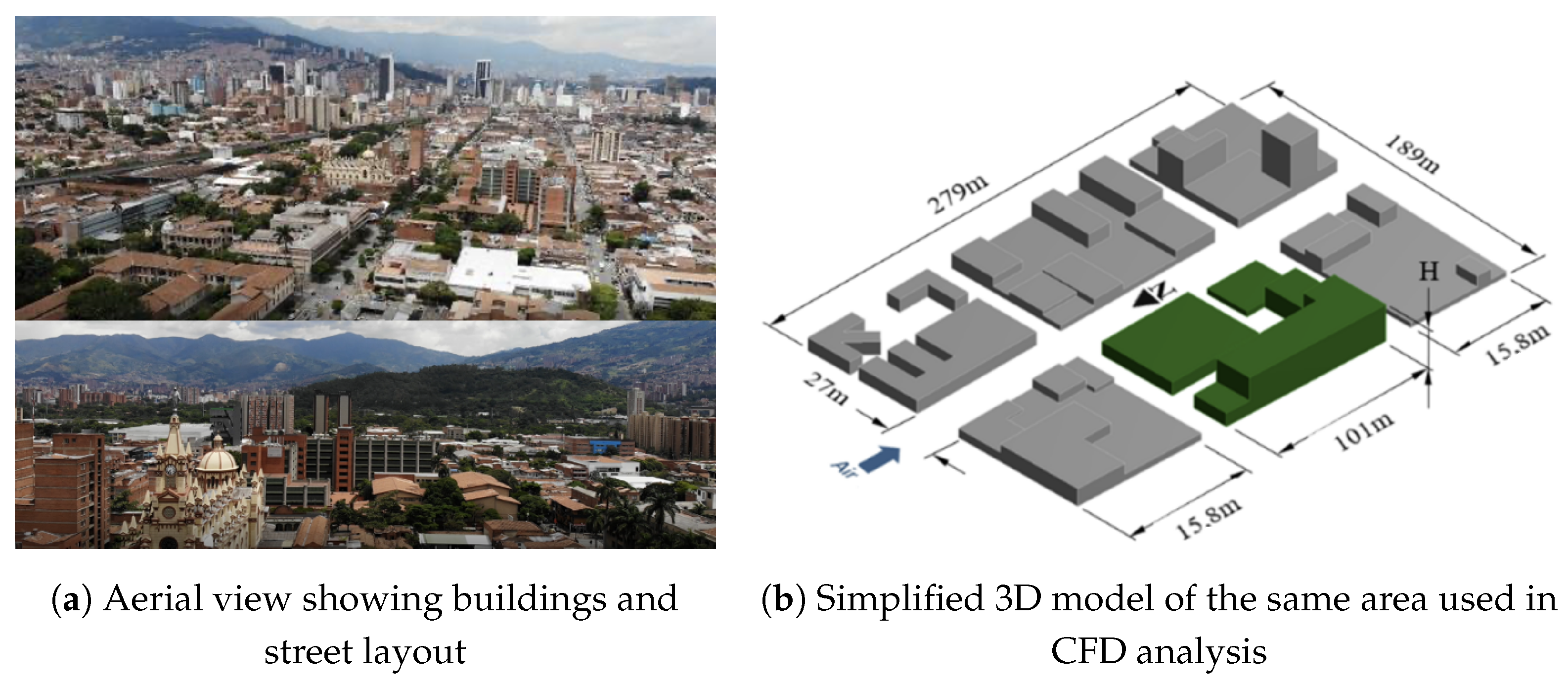
The study area is made up of six blocks consisting of buildings of different heights and separated by streets. Figure 1 shows the aerial view and the lateral view of the study area, respectively. It is possible to observe the University of Antioquia core research center (SIU for its Spanish acronym).

It is also possible to observe the Faculty of Medicine located in the N-E block (27 $\mathrm{m}$ × $15.8$ $\mathrm{m}$) and the Faculty of Odontology located in the N-W block just next to the Faculty of Medicine. Both faculties belong to the University of Antioquia. The above-mentioned urban interventions were constructed during different periods of time in a residential area and are considered individual units separated by public streets. It is also possible to observe the different architectural configurations adopted by the University of Antioquia for those interventions. To conduct the CFD simulation, the architectural details of the buildings considered in the study area were simplified using simple geometric figures for their representation. In this study, the main reference corresponds to the Faculty of Medicine and the SIU research center, which has a reference height H of 30 $\mathrm{m}$ (Figure 1).

Wind direction, as shown in Figure 2, is defined perpendicular to the main building of the SIU research center in the N-S direction (greater prevalence of wind direction for the Aburrá Valley). The measurements of the concentration of atmospheric pollutants were obtained from monitoring station 6 (Siata) located to the north and closest to the study area during three periods and for the entire month of April 2018. These recorded values were averaged to validate the computational model. It is important to note that the street in the N-S direction is named Carabobo and has been subjected to different urban interventions. In the central area of Medellín, the Carabobo Street became in recent years a pedestrian street. Therefore, pollutants produced by vehicular combustion or accidental discharges in the area of study were not considered in the CFD model in order to study the current pollutant dispersion in the street because there are plans to convert other portions of the Carabobo Street (including the one considered in this study) into a pedestrian street. In addition, the University of Antioquia is currently planning the construction of new infrastructure in the area of study in order to provide new research facilities to the SIU research center. Urban intervention considers the construction of new pedestrian areas as well for users of the SIU research center.

3.2. Computational Domain

The computational domain used in the present work considers an upstream distance, between the inlet of the computational domain and the buildings, of 20H, to limit the development of the input gradients. The downstream distance, between the buildings and the outlet of the computational domain, corresponds to 60H. The lateral distances of the computational domain extend 16H, from the outer buildings to the lateral borders of the computational domain. The height of the computational domain is 8H, which is approximately equal to the height of the boundary layer of the terrain. The final dimensions of the computational domain are 1144 × 240 × 2678 [m] (X, Y, Z). Adequate modeling of the building area requires the definition of a subdomain to obtain greater precision in the solution. The dimensions of the computational subdomain are therefore 11H × 3H × 14H (X, Y, Z). The computational domain and corresponding boundary conditions are shown in Figure 2. To fully define the flow simulation, Dirichlet boundary conditions are set on the domain surfaces. For the upper border and the lateral borders of the domain, the symmetry condition is used, which considers a normal velocity and a gradient equal to zero in all the variables on the symmetry plane. For the exit boundary, an outflow condition is used, which considers that the flow is fully developed, and the variables of interest do not change in the direction of the flow. For the floor and walls of buildings, a no-slip condition is implemented, which uses wall functions to consider the effect of roughness.

Inlet boundary: Vertical velocity profile (north side). Outlet: Outflow condition (south side). Lateral and top boundaries: Symmetry. Bottom and walls: No-slip condition with surface roughness. Domain dimensions: 1144 m (X) × 240 m (Y) × 2678 m (Z). The subdomain was defined to focus the mesh refinement in the area of interest (buildings and urban interventions), optimizing the resolution of local flows and pollutant dispersion, while reducing the overall computational cost.

Finally, for the input boundary of the computational domain, user-defined functions (UDFs) are used to enter the profiles of velocity, turbulent kinetic energy, and the turbulent dissipation rate as a function of the height of the domain. These aspects will be further discussed.

3.3. Hybrid RANS/LES Modeling Approach

To address the multi-scale nature of urban pollutant dispersion, we employed a hybrid modeling approach combining RANS and LES simulations. The steady-state RANS (SST $\kappa -\omega$) model provided computationally efficient analysis of mean flow patterns and bulk ventilation characteristics across the full domain, consistent with established urban CFD practices [21]. For critical zones identified by RANS (e.g., pedestrian-level recirculation areas), we applied LES with dynamic Smagorinsky closure to resolve the transient turbulence effects and instantaneous pollutant peaks. This dual-methodology strategy was validated against field measurements, showing <15% variation in the key metrics (e.g., $1.2\pm 0.3$ m/s vs. 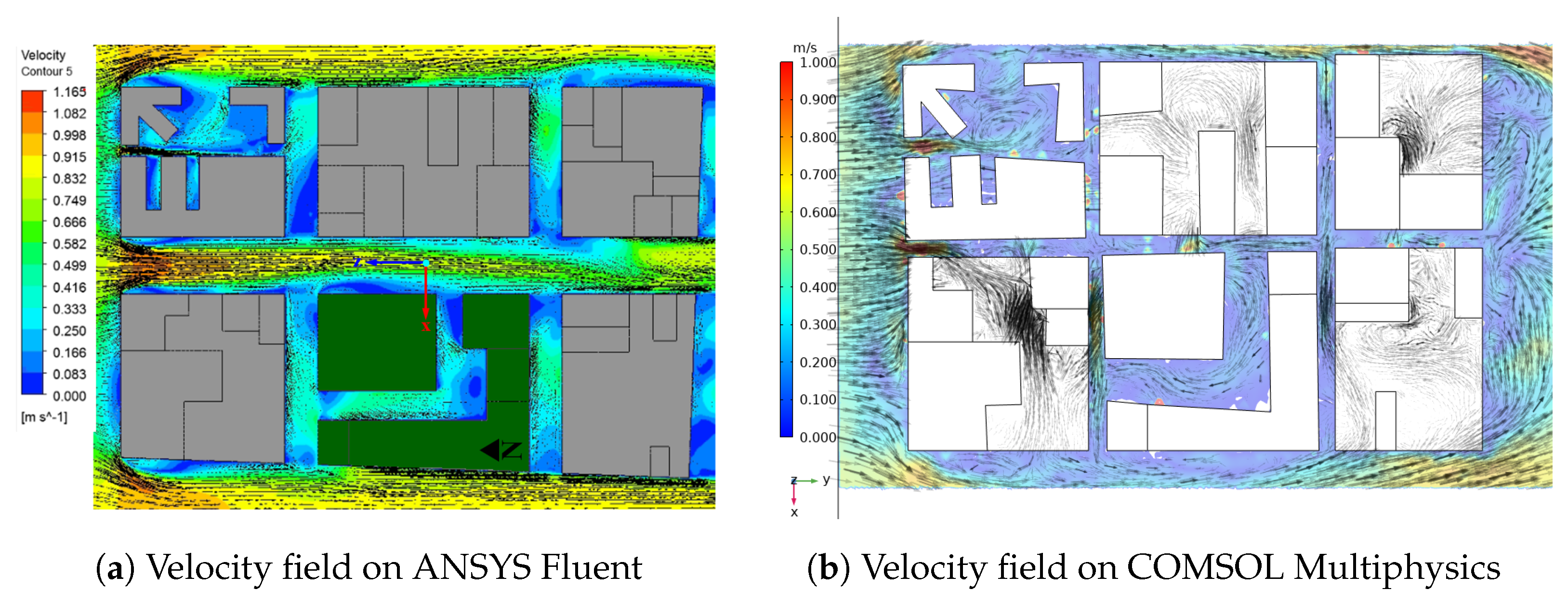$1.0\pm 0.4$ m/s for pedestrian-level winds). The complementary use of ANSYS 2022 Fluent (RANS) and COMSOL Multiphysics (LES) leveraged each software’s strengths: Fluent’s robust industrial-scale solver for baseline analysis, and COMSOL’s adaptive meshing and multiphysics coupling for complex near-building dynamics. Cross-validation confirmed solution consistency, with runtime trade-offs (48 vs. 62 core-hours) justifying the targeted LES deployment. In

Table 2. Comparison of RANS (Fluent), LES (COMSOL), and field data results. Relative difference is calculated between RANS and LES models.

Parameter	RANS (Fluent)	LES (COMSOL)	Field Data	Relative Difference (RANS vs. LES)
Flow Characteristics
Pedestrian-level wind speed (m/s)	1.22 ± 0.25	1.18 ± 0.41	1.15 ± 0.33	3.4%
Turbulent kinetic energy (${\mathrm{m}}^2$/${\mathrm{s}}^2$)	0.47	0.52	–	10.6%
Pollutant Dispersion
Mean ${\mathrm{NO}}_2$ ($\mathsf{\mu }$g/${\mathrm{m}}^3$)	38.2	41.7	39.5 ± 8.3	9.2%
Peak ${\mathrm{NO}}_x$ ($\mathsf{\mu }$g/${\mathrm{m}}^3$)	52.1	58.3	–	11.9%
Computational Cost
Mesh resolution (million cells)	3.8	6.2	–	63%
Simulation time (core-hours)	48	62	–	29.2%

, the key parameters and results from both RANS and LES simulations were summarized, highlighting the effectiveness of this hybrid approach in capturing pollutant dispersion dynamics across urban environments.

3.4. Model Implementation

The turbulent flow in the study area was modeled using the Large Eddy Simulation (LES) approach with the Smagorinsky subgrid-scale (SGS) model in COMSOL Multiphysics. Given the complex urban geometry of Medellín’s street canyon—characterized by heterogeneous building heights, pedestrian zones, and narrow passages—the LES–Smagorinsky model was selected to resolve large-scale eddies while parameterizing smaller. The Smagorinsky constant ($C_s$) was set to $0.5$, a value empirically validated for urban airflow studies, to compute the eddy viscosity as $v_t={\left(C_s\mathsf{\Delta }\right)}^2\sqrt{2S_{ij}{S}_{ij}}$, where $\mathsf{\Delta }$ represents the local grid filter width and $S_{ij}{S}_{ij}$ is the strain-rate tensor. The computational mesh was refined near building surfaces and pedestrian-level zones (2 m height) to resolve critical flow features, such as recirculation vortices and shear layers, while ensuring a $y^{+}<30$ to align with the LES requirements. Inlet boundary conditions incorporated a neutral atmospheric boundary layer profile, with the turbulence intensity adjusted to match field measurements from the Siata monitoring network. Wall functions accounted for surface roughness ($k_s=0.064$ m) to replicate realistic urban drag effects. This setup enabled the high-fidelity prediction of NO_x dispersion patterns, particularly in low-velocity zones induced by recent pedestrian-oriented interventions, while balancing computational efficiency and accuracy for the geometrically intricate domain.

3.5. Mesh Sensitivity Analysis

An adequate computational mesh is necessary in order to guarantee a good representation of velocity profiles, and concentrations of atmospheric pollutants around buildings, among other factors. The domain was discretized using the Cartesian cut-cell method. This method of mesh construction allows better control of the size relationships, with very fine meshes near the walls of the buildings to thicker meshes in the areas furthest from the area of interest as shown in Figure 1. It is important to note that the size of the elements on the floor surfaces and the walls of the buildings are defined to comply with the value of $y^{+}>30$ in all mesh configurations.

An analysis of mesh independence defined for the computational domain is performed using six mesh densities, which are generated in order to guarantee the mesh independence from the results obtained around the buildings. The north and south wind speeds are also considered in the sub-domain on the Y-Z plane as shown in Figure 3. Based on the above-mentioned, it is found that the speeds do not show significant changes when there are around $3.8$ million elements in the domain. Therefore, this distribution provides a good balance between computational cost and numerical uncertainty. Courant numbers $<1$ ensure stability in transient simulations.

3.6. Physical Model

ANSYS Fluent software is used to solve the RANS equations in the steady state in three dimensions using the SST $\kappa -\omega$ turbulence model. The SIMPLE algorithm is used for velocity–pressure coupling. An upwind second-order scheme is implemented for the convective term in order to improve the numerical precision, except for pressure. In addition, the convergence criterion is established when the residuals reach a value equal to or less than $1\times {10}^{-5}$, a value frequently reported in the literature. For all the case studies, about 2100 iterations are required to obtain a convergence in the solution. The calculations are carried out on a parallel vector computer using sixteen Intel (R) Xeon (R) processors (CPUE5-2667 @ $2.90$ GHz) and 64 Gb of RAM with a 64-bit operating system.

3.7. Physical Model

The validation of the CFD model is carried out by taking the mass fraction for ${\mathrm{NO}}_2$ and NO at two points, one at the entrance and the other at the exit of the area of interest, and compared with the data reported by Siata. The standard deviation of the measurements collected in one month is calculated in order to determine the error. At the entrance of the computational domain, values of $6.693\times {\mathrm{10}}^{-9}$ $\mathsf{\mu }$$\mathrm{g}$ and $1.541\times {\mathrm{10}}^{-8}$ $\mathsf{\mu }$$\mathrm{g}$ are used for NO and ${\mathrm{NO}}_2$, respectively. On the other hand, values of $1.788\times {\mathrm{10}}^{-8}$ $\mathsf{\mu }$$\mathrm{g}$ and $1.984\times {\mathrm{10}}^{-8}$ $\mathsf{\mu }$$\mathrm{g}$ are used at the exit of the computational domain for NO and ${\mathrm{NO}}_2$, respectively. Figure 3 shows good agreement between the experimental and CFD results at the entrance with a maximum relative error value of 2.95%. However, at the exit there is a relative error for nitric oxide of 8.11% and for nitrogen dioxide of 30.42%. The difference between the data reported experimentally and the data obtained in the CFD simulations is due, in large part, to the atmospheric changes near the sites where the measurements were collected. Finally, the data entered into the computational model do not show these variations. In recent work, the incorporation of artificial intelligence algorithms has improved the prediction of transport of complex contaminants, complementing traditional CFD simulations [22,23].

4. Results

Figure 4 shows that the wind flow field is represented by velocity vectors and velocity contours at a height of 2 $\mathrm{m}$ in a horizontal section. It is also possible to observe that the highest wind speeds are parallel to the input wind speed. Recirculation vortices are present at road crossings, close to the intersections and parallel to the x-axis; this vortex is not present along the entire street. In the corner vortices, there is a helical structure that transports the pollutants from the streets between the buildings to where the main wind flow is, parallel to the z-axis. It is important to note that the wind speeds along the x and z axes do not have a clear pattern along their path, due to the lack of uniformity in the shape and height of the buildings. Wind predominantly blows from north to south.

As shown in Figure 4b, the presence of turbulent flow is more pronounced in areas where buildings are located. This is due to the non-uniform distribution of wind speed along the street: higher wind speeds are observed at the entrance of the street, where no buildings are present, while lower wind speeds occur near the buildings due to flow obstruction. This phenomenon, known as wind shadowing, leads to the recirculation of air and pollutants within the shared spaces of the buildings—areas where people typically gather and move. The resulting stagnation of air can significantly impact pollutant dispersion in urban environments and increase the potential health risks for people in these zones.

The average wind velocity at the pedestrian level is drastically reduced in the west side of the street canyon right behind the Faculty of Medicine. The same pattern is also observed in SIU research center, especially in the pedestrian zone located in the east entrance of the SIU research center. Figure 5 shows the step-down street canyon right behind the Faculty of Medicine. Voodeckers et al. (2021) stated that the ratio of the building height to the street width (H/W ratio), also known as the Aspect Ratio (AR), has a threshold value of $0.65$; values of AR larger than $0.65$ produce a sharp reduction in the pollutant exchange rate, and the ventilation capacity cannot be guaranteed [3]. It is possible to observe in Figure 5 that the urban intervention conducted by the University of Antioquia using a configuration with $\mathrm{AR}>0.65$ results in insufficient ventilation capacity in the step-down street canyon right behind the Faculty of Medicine.

Insufficient ventilation capacity is also observed in the pedestrian zone located in the east entrance of the SIU research center as shown in Figure 4. Voodeckers et al. (2021) stated that the street canyon depth has a threshold value of $5.0$. The SIU research center currently presents in some pedestrian zones’ values of AR larger than $5.0$ [3]. Therefore, special measures must be taken to ensure sufficient ventilation for new building construction in the SIU research center area. 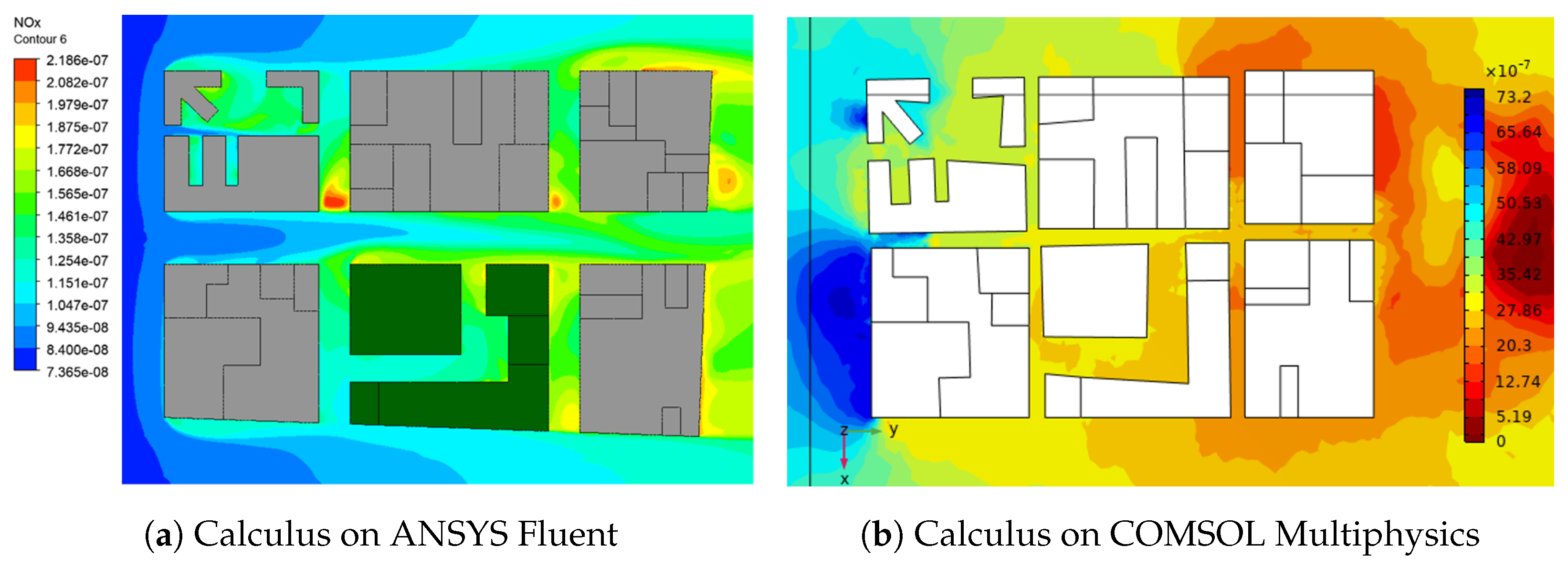Figure 6 shows the horizontal section of ${\mathrm{NO}}_x$ concentrations at a height of 2 $\mathrm{m}$. It is possible to observe that ${\mathrm{NO}}_x$ concentrations are larger in the above-mentioned areas where low wind speed is evident based on the simulation results.

Wind blows from north to south, and therefore pollutants emitted from vehicles are dragging in that direction, but the situation is critical since the two above-mentioned areas promote deposited ${\mathrm{NO}}_x$. Sánchez et al. (2021) stated that lower wind speed increases the residence time of ${\mathrm{NO}}_x$ [11]. Although no vehicle emissions are included in the CFD model presented in this paper, it is clear that even if the Carabobo Street in the near future is defined as pedestrian-only use, special measures have to be taken to reduce the residence time of ${\mathrm{NO}}_x$, considering the limitations of the local mitigation approaches presented in this paper. In the central area of Medellín, some parts of the Carabobo Street are defined as pedestrian-only use. Therefore, vehicle access restriction is expected in the near future due to the active urban intervention that is currently under process in the area of study and the necessity to have areas for pedestrians.

As previously mentioned, the Aburrá Valley, Medellín, is a narrow tropical valley with strong thermal inversion and unstable atmospheric conditions. In addition, the annual concentration of ${\mathrm{NO}}_2$ has remained basically unaltered in Medellín over the last 8 years, showing a peak of $37.7$ $\mathsf{\mu }$$\mathrm{g}$/${\mathrm{m}}^3$ ± $8.3$ $\mathsf{\mu }$$\mathrm{g}$/${\mathrm{m}}^3$, a value close to the findings of Zhao et al. (2021), who reported two ${\mathrm{NO}}_2$ concentration critical values of 43 $\mathsf{\mu }$$\mathrm{g}$/${\mathrm{m}}^3$ and 48 $\mathsf{\mu }$$\mathrm{g}$/${\mathrm{m}}^3$ for increasing risk of cardiovascular and respiratory mortality [7].

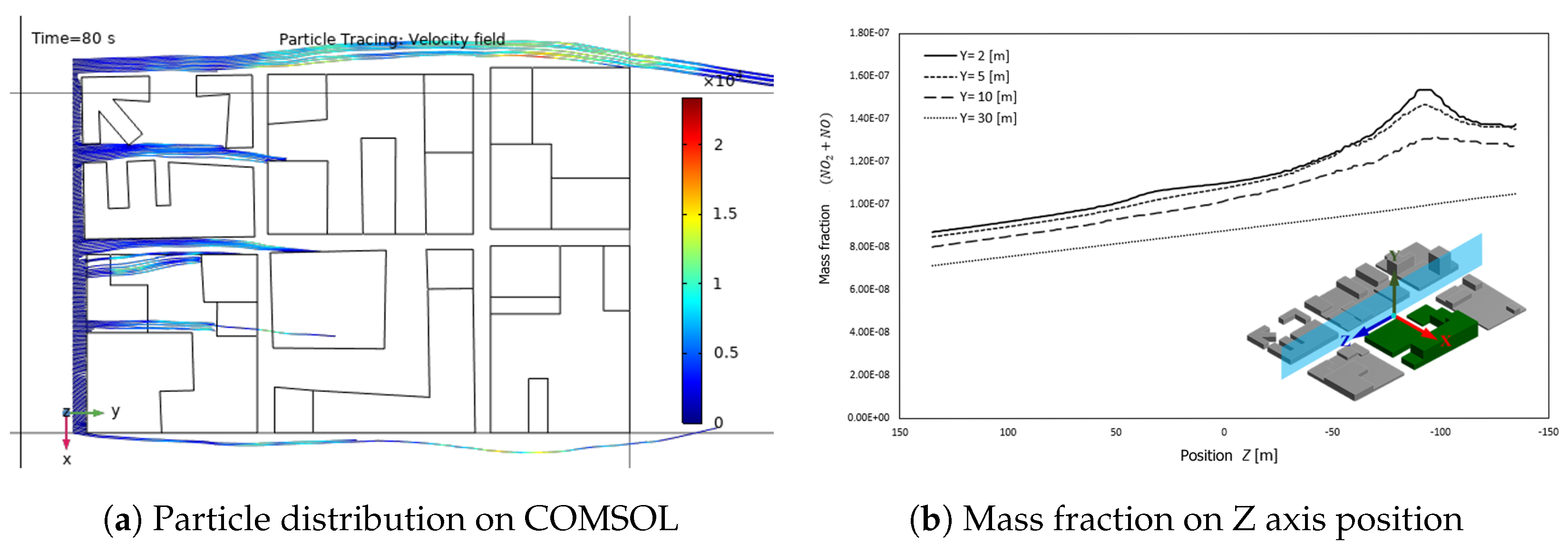
Therefore, public urban intervention must address the full-scale implementation of passive actions to control traffic-related air pollution, especially in areas that during the last years have been gradually converted in pedestrian areas. Finally, Figure 7 shows the concentration of ${\mathrm{NO}}_2$ plus NO along the $Y-Z$ plane, for different heights; $Y=2$, 5, 10, and 30 $\mathrm{m}$. Due to the diffusion phenomenon caused by turbulent vortices, the concentration of pollutants tends to be higher at ground level ($Y=2$ $\mathrm{m}$). Akhatova et al. (2016) using CFD simulation conducted a study of carbon monoxide (CO) dispersion in a crossroad street in Astana and pointed out that pedestrians are exposed to higher CO concentration levels in comparison with the inhabitants of buildings [15].

5. Discussion and Conclusions

This study aimed to evaluate the impact of recent urban interventions on NO_x dispersion in a representative street canyon of Medellín, Colombia. The simulation results, validated against field measurements, provide insight into airflow dynamics, pollutant accumulation patterns, and potential areas of concern within the modeled domain. The following discussion analyzes the key findings in light of the study’s objectives, highlights the limitations of the modeling approach, and proposes recommendations for improving both future simulations and urban design strategies. Particular attention is given to the causes of discrepancies observed between the model predictions and field data, the influence of morphological features on pollutant retention, and the implications of vegetation placement in pedestrian areas.

The relatively high relative error observed for ${\mathrm{NO}}_2$ at the outlet boundary (30.42%) is primarily attributed to two key factors. First, the atmospheric conditions were simplified in the model by assuming a stationary boundary layer profile without accounting for temporal variability in the meteorological parameters such as wind speed, temperature, and humidity. These parameters, known to exhibit fluctuations throughout the day due to thermal inversion and topographical effects in the Aburrá Valley [24], are critical in influencing the pollutant dispersion. Such simplifications likely limited the model’s ability to reproduce transient dispersion patterns accurately, particularly in a complex urban environment like Medellín, where strong diurnal variations and unstable boundary layers are common [25]. Second, the model deliberately excluded vehicular emissions to focus on the impact of the recent urban interventions on ${\mathrm{NO}}_x$ dispersion. While this approach allows a clearer assessment of morphological influences, it inherently omits a significant source of ${\mathrm{NO}}_x$ in urban areas [1], potentially underestimating the localized pollutant concentrations and their variability. These two factors combined contribute to the discrepancies observed, particularly at the outlet boundary, where atmospheric dilution and emission sources downstream of the domain may also play a role. Future work should incorporate dynamic meteorological inputs, transient simulations under varying atmospheric stability classes, and explicit traffic emission sources to improve model fidelity and predictive accuracy in real-world conditions [2,11].

The average wind velocity at the pedestrian level was significantly reduced behind the Faculty of Medicine, particularly along the western side of the street canyon. A similar reduction was observed at the east entrance of the SIU Research Center. As shown in Figure 4, the urban configuration behind the Faculty of Medicine corresponds to a step-down street canyon. According to Voordeckers et al. (2021), a height-to-width ratio (H/W or Aspect Ratio, AR) greater than $0.65$ leads to a marked reduction in pollutant exchange and insufficient ventilation capacity [3]. In the studied configuration, AR values exceed this threshold, suggesting that the urban intervention implemented by the University of Antioquia resulted in suboptimal air circulation.

Additionally, low ventilation was also detected in the pedestrian area at the eastern entrance of the SIU Research Center, where AR values exceeded $5.0$ in some locations—well above the threshold defined by Voordeckers et al. (2021) for adequate air exchange in deep canyons [3]. As visualized in Figure 6, ${\mathrm{NO}}_x$ concentrations were highest in these low-wind-speed areas. Although vehicle emissions were excluded from the CFD model, the results clearly show that even pedestrian-only zones may suffer from pollutant retention due to poor ventilation conditions.

These findings emphasize the need for improved urban planning strategies that consider airflow and pollutant dispersion, especially in areas undergoing transformation into pedestrian corridors. In the context of Medellín’s atmospheric conditions—characterized by frequent thermal inversions and limited vertical mixing—ensuring adequate ventilation becomes critical to reduce ${\mathrm{NO}}_x$ residence time and improve urban air quality.

The simulation results also indicate elevated ${\mathrm{NO}}_x$ concentrations in areas with vegetation, particularly around the Faculty of Medicine where several trees are located. While urban greenery is typically associated with benefits such as thermal regulation and energy savings, its impact on airflow in dense urban canyons can be counterproductive. As reported by Voordeckers et al. (2021), dense tree canopies can obstruct wind flow and reduce air exchange rates, potentially increasing pollutant residence time [3]. In this study, vegetation appears to contribute to the formation of low-velocity zones, thereby enhancing localized ${\mathrm{NO}}_x$ accumulation. These findings suggest that tree planting in street canyons should be carefully evaluated to balance environmental benefits with ventilation and air quality considerations.

Based on these observations, future modeling efforts should incorporate key improvements to enhance predictive accuracy and reliability. Firstly, it is recommended to include vehicular emissions in the simulations, using available traffic flow data, emission factors, and temporal profiles, as these sources represent a major contributor to ${\mathrm{NO}}_x$ levels in urban environments [3,11]. Secondly, implementing time-dependent boundary conditions that account for diurnal and seasonal variability in meteorological parameters—such as wind direction, wind speed, atmospheric stability, and temperature gradients—would provide a more realistic representation of pollutant dispersion, particularly in complex topographies like the Aburrá Valley [2,24]. Additionally, coupling the CFD model with local air quality monitoring networks for continuous calibration and validation is strongly suggested to minimize model uncertainties and improve the interpretation of results [25]. These enhancements would strengthen the model’s capability to inform urban planning decisions, especially in the design of pedestrian areas and urban interventions aimed at reducing pollutant exposure.

To improve the validation of CFD models in complex urban environments such as Medellín, we propose a field study design that includes simultaneous measurements of ${\mathrm{NO}}_x$ concentrations, wind speed, and wind direction at multiple heights and locations within the street canyon. Specifically, measurement points should be installed at the pedestrian level (2 $\mathrm{m}$), mid-height (10 $\mathrm{m}$), and rooftop level (30 $\mathrm{m}$), following the established protocols for vertical profiling in urban air quality monitoring [25]. Data collection should be conducted continuously over several weeks to capture diurnal and meteorological variability, with a focus on periods of known thermal inversion. This approach will enable a more robust calibration and validation of CFD simulations, ensuring that future urban design interventions account for real-world dispersion patterns and pollutant accumulation hotspots. Collaboration with the local air quality monitoring network (SIATA) and urban planning authorities is essential to implement these measurements effectively.

Overall, this study demonstrates the critical role of urban morphology, airflow dynamics, and vegetation placement in shaping pollutant accumulation within pedestrian zones. By incorporating these findings into urban planning practices and strengthening model validation through field measurements, future interventions can be designed to mitigate air pollution exposure and improve public health outcomes in dense urban areas.