

Sustainable Crop Farm Productivity: Weather Effects, Technology Adoption, and Farm Management


Abstract
1. Introduction
2. Methods
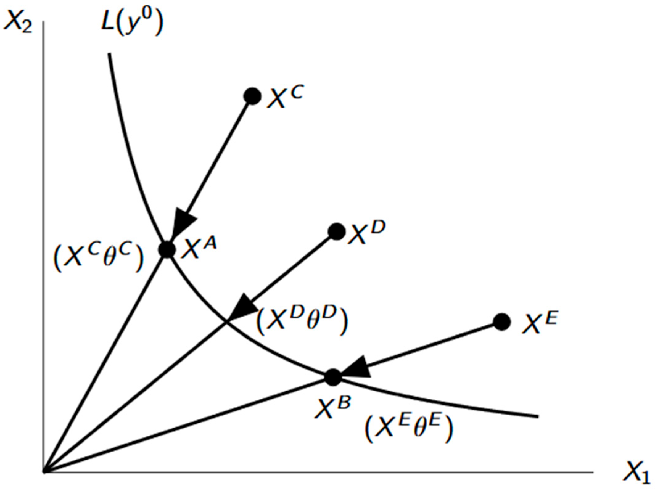
2.1. Theoretical Framework
2.2. Potential Endogeneity Issues and Assumptions
2.3. Farm Financial Data
2.4. Farm Management Practices and Technology Adoption Data
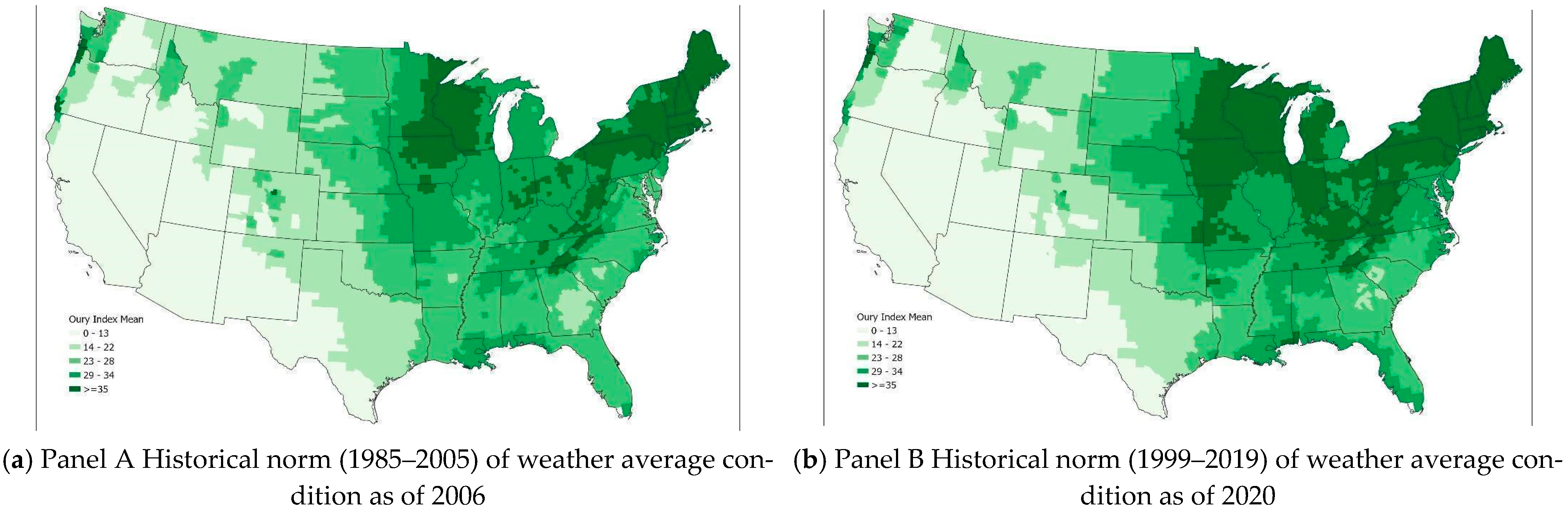
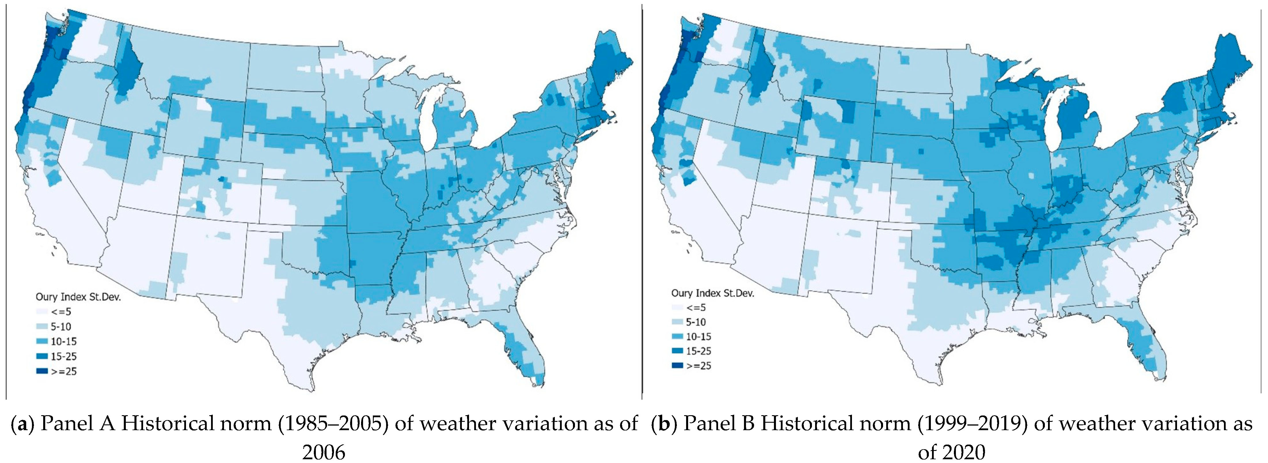
2.5. Weather and Climate Variables
3. Results and Discussion
3.1. Climatic Effects and Field Crop Farm Productivity
3.2. Impacts of Technology Adoption and Farm Management Practices on Field Crop Farm Productivity
4. Conclusions
Author Contributions
Funding
Institutional Review Board Statement
Informed Consent Statement
Data Availability Statement
Acknowledgments
Conflicts of Interest
References
- United Nations. World Population Prospects: The 2024 Revision. Available online: www.un.org (accessed on 3 July 2025).
- Coomes, O.T.; Barham, B.L.; MacDonald, G.K.; Ramankutty, N.; Chavas, J. Leveraging Total Factor Productivity Growth for Sustainable and Resilient Farming. Nat. Sustain. 2019, 2, 22–28. [Google Scholar] [CrossRef]
- Wang, S.L.; Heisey, P.; Schimmelpfennig, D.; Ball, V.E. Agricultural Productivity Growth in the United States: Measurement, Trends, and Drivers; Paper No. ERR-18; USDA Economic Research Service: Washington, DC, USA, 2015.
- Semenov, M.A.; Porter, J.R. Climatic Variability and the Modelling of Crop Yields. Agric. For. Meteorol. 1995, 73, 265–283. [Google Scholar] [CrossRef]
- Ferris, R.; Ellis, R.H.; Wheeler, T.R.; Hadley, P. Effect of High Temperature Stress at Anthesis on Grain Yield and Biomass of Field-Grown Crops of Wheat. Ann. Bot. 1998, 82, 631–639. [Google Scholar] [CrossRef]
- Miao, R.; Khanna, M.; Huang, H. Responsiveness of Crop Yield and Acreage to Prices and Climate. Am. J. Agric. Econ. 2016, 98, 191–211. [Google Scholar] [CrossRef]
- Aragón, F.M.; Oteiza, F.; Rud, J.P. Climate Change and Agriculture: Subsistence Farmers’ Response to Extreme Heat. Am. Econ. J. Econ. Policy 2021, 13, 1–35. [Google Scholar] [CrossRef]
- Carter, T.R.; Parry, M.L.; Harasawa, H.; Nishioka, S. IPCC Technical Guidelines for Assessing Climate Change Impacts and Adaptations; Department of Geography, University College London: London, UK; Center for Global Environmental Research, National Institute for Environmental Studies: Tsukuba-City, Japan, 1994. [Google Scholar]
- Lobell, D.B.; Asner, G.P. Climate and Management Contributions to Recent Trends in U.S. Agricultural Yields. Science 2003, 299, 1032. [Google Scholar] [CrossRef] [PubMed]
- Schlenker, W.; Roberts, M.J. Nonlinear Temperature Effects Indicate Severe Damages to US Crop Yield under Climate Change. Proc. Natl. Acad. Sci. USA 2009, 106, 15594–15598. [Google Scholar] [CrossRef] [PubMed]
- Ortiz-Bobea, A.; Knippenberg, E.; Chambers, R.G. Growing Climatic Sensitivity of US Agriculture Linked to Technological Change and Regional Specialization. Sci. Adv. 2018, 4, eaat4343. [Google Scholar] [CrossRef] [PubMed]
- Brisson, N.N.; Philippe, P.G.; Gouache, D.D.; Charmet, G.; Oury, F.-X.; Huard, F. Why are Wheat Yields Stagnating in Europe? A Comprehensive Data Analysis for France. Field Crops Res. 2010, 119, 201–212. [Google Scholar] [CrossRef]
- Zhong, Z.; Hu, Y.; Jiang, L. Impact of Climate Change on Agricultural Total Factor Productivity Based on Spatial Panel Data Model: Evidence from China. Sustainability 2019, 11, 1516. [Google Scholar] [CrossRef]
- Li, H.; Liu, H. Climate Change, Farm Irrigation Facilities, and Agriculture Total Factor Productivity: Evidence from China. Sustainability 2023, 15, 2889. [Google Scholar] [CrossRef]
- Saavoss, M.; Capehart, T.; McBride, W.; Effland, A. Trends in Production Practices and Costs of the U.S. Corn Sector; Economic Research Report No. ERR-294; USDA Economic Research Service: Washington, DC, USA, 2021.
- Zhang, B.; Carter, C.A. Reforms, the Weather, and Productivity Growth in China’s Grain Sector. Am. J. Agric. Econ. 1997, 79, 1266–1277. [Google Scholar] [CrossRef]
- Zhang, B.; Wang, G.; Liu, X. Research on Corn and Soybean Rotation: A Review of Ecological Benefits and Economic Potential. Resour. Data J. 2024, 3, 208–222. [Google Scholar]
- Bullock, D.G. Crop Rotation. Crit. Rev. Plant Sci. 1992, 11, 309–326. [Google Scholar] [CrossRef]
- Zhang, H.; Mu, J.E.; McCarl, B.A. Adaptation to Climate Change through Fallow Rotation in the U.S. Pacific Northwest. Climate 2017, 5, 64. [Google Scholar] [CrossRef]
- Schimmelpfennig, D. Farm Profits and Adoption of Precision Agriculture; Economic Research Report No. ERR-217; USDA Economic Research Service: Washington, DC, USA, 2016.
- McFadden, J.; Smith, D.; Wechsler, S.; Wallander, S. Development, Adoption, and Management of Drought-Tolerant Corn in the United States; USDA Economic Research Service Economic Information Bulletin: Washington, DC, USA, 2019; Report Number 204.
- King, K.W.; Williams, M.R.; Fausey, N.R. Contributions of Systematic Tile Drainage to Watershed-Scale Phosphorus Transport. J. Environ. Qual. 2015, 44, 486–494. [Google Scholar] [CrossRef] [PubMed]
- Meyer, K.; Keiser, D.A. Adapting to Climate Change through Tile Drainage: Evidence from Micro Level Data. In Proceedings of the 2016 Annual Meeting, Boston, MA, USA, 31 July–2 August 2016; Agricultural and Applied Economics Association: Milwaukee, WI, USA, 2016. [Google Scholar]
- Yang, S.; Shumway, C.R. Dynamic Adjustment in U.S. Agriculture under Climate Change. Am. J. Agric. Econ. 2015, 98, 910–924. [Google Scholar] [CrossRef]
- Liang, X.; Wu, Y.; Chambers, R.G.; Schmoldt, D.L.; Gao, W.; Liu, C.; Liu, Y.; Sun, C.; Kennedy, J.A. Determining Climate Effects on U.S. Total Agricultural Productivity. Proc. Natl. Acad. Sci. USA 2017, 114, E2285–E2292. [Google Scholar] [CrossRef] [PubMed]
- Njuki, E.; Bravo-Ureta, B.E.; O’Donnell, C.J. A New Look at the Decomposition of Agricultural Productivity Growth Incorporating Weather Effects. PLoS ONE 2018, 13, e0192432. [Google Scholar] [CrossRef] [PubMed]
- Wang, S.L.; Ball, V.E.; Nehring, R.; Williams, R.; Chau, T. Chapter 2—Impacts of Climate Change and Extreme Weather on US Agricultural Productivity: Evidence and Projection. In Agricultural Productivity and Behavior; Schlenker, W., Ed.; NBER; University of Chicago Press: Chicago, IL, USA, 2019. [Google Scholar]
- Chambers, R.G.; Pieralli, S. The Sources of Measured US Agricultural Productivity Growth: Weather, Technological Change, and Adaption. Am. J. Agric. Econ. 2020, 102, 1198–1226. [Google Scholar] [CrossRef]
- Simar, L.; Wilson, P.W. Estimation and Inference in Two-Stage, Semi-Parametric Models of Production Processes. J. Econom. 2007, 136, 31–64. [Google Scholar] [CrossRef]
- Fare, R.; Primont, D. The Unification of Ronald W. Shephard’s Duality Theory. J. Econ. 1990, 60, 199–207. [Google Scholar] [CrossRef]
- Lovell, C.; Richarson, S.; Travers, P.; Wood, L. Resources and Functionings: A New View of Inequality in Australia. In Models and Measurement of Welfare and Inequality; Eichhorn, W., Ed.; Springer: Berlin/Heidelberg, Germany, 1994; pp. 787–807. [Google Scholar]
- Kumbhakar, S.C.; Lovell, C.A.K. Stochastic Frontier Analysis, 2nd ed.; Cambridge University Press: Cambridge, UK, 2004. [Google Scholar]
- Kumbhakar, S.C.; Orea, L.; Rodríguez-Álvarez, A.; Tsionas, E.G. Do We Estimate an Input or an Output Distance Function? An Application of the Mixture Approach to European Railways. J. Product. Anal. 2007, 27, 87–100. [Google Scholar] [CrossRef]
- Battese, G.; Coelli, T. Frontier Production Functions, Technical Efficiency, and Panel Data: With Application to Paddy Farmers in India. J. Product. Anal. 1992, 3, 153–169. [Google Scholar] [CrossRef]
- Burbidge, J.B.; Magee, L.; Robb, A.L. Alternative Transformations to Handle Extreme Values of the Dependent Variable. J. Am. Stat. Assoc. 1998, 83, 123–127. [Google Scholar] [CrossRef]
- Zellner, A.; Kmenta, J.; Dreze, J. Specification and Estimation of Cobb-Douglas Production Function Models. Econometrica 1966, 34, 784–795. [Google Scholar] [CrossRef]
- Schlenker, W.; Roberts, M.J. Nonlinear Effects of Weather on Corn Yields. Rev. Agric. Econ. 2006, 28, 391–398. [Google Scholar] [CrossRef]
- Auffhammer, M.; Hsiang, S.M.; Schlenker, W.; Sobel, A. Using Weather Data and Climate Model Output in Economic Analyses of Climate Change. Rev. Environ. Econ. Policy 2013, 7, 181–198. [Google Scholar] [CrossRef]
- USDA-ERS ARMS Farm Financial and Crop Production Practices Documentation. Available online: https://www.ers.usda.gov/data-products/arms-farm-financial-and-crop-production-practices/documentation/ (accessed on 25 June 2025).
- Wang, S.L.; Rada, N.; Williams, R.; Newton, D. Accounting for Climatic Effects in Measuring U.S. Field Crop Farm Productivity. Appl. Econ. Perspect. Policy 2022, 44, 1975–1994. [Google Scholar] [CrossRef]
- Schimmelpfennig, D.; Ebel, R. On the Doorstep of the Information Age: Recent Adoption of Precision Agriculture; USDA Economic Research Service Economic Information Bulletin: Washington, DC, USA, 2011; Report Number 80. [Google Scholar]
- Rejesus, R.M.; Marra, M.C.; Roberts, R.K.; English, B.C.; Larson, J.A.; Paxton, K.W. Changes in Producers’ Perceptions of Within-Field Yield Variability after Adoption of Cotton Yield Monitors. J. Agric. Appl. Econ. 2013, 45, 295–312. [Google Scholar] [CrossRef]
- Paltasingh, K.R.; Goyari, P.; Mishra, R.K. Measuring Weather Impact on Crop Yield Using Aridity Index: Evidence from Odisha. Agric. Econ. Res. Rev. 2012, 25, 205–216. [Google Scholar]
- Daly, C.; Halbleib, M.; Smith, J.; Gibson, W.; Doggett, M.; Taylor, G.; Curtis, J.; Pasteris, P. Physiographically Sensitive Mapping of Climatological Temperature and Precipitation Across the Conterminous United States. Int. J. Climatol. 2008, 28, 2031–2064. [Google Scholar] [CrossRef]
- PRISM Climate Group, Oregon State University. Available online: https://prism.oregonstate.edu (accessed on 1 October 2021).
- McFadden, J.R.; Rosberg, A.; Njuki, E. Information Inputs and Technical Efficiency in Midwest Corn Production: Evidence from Farmers’ Use of Yield and Soil Maps. Am. J. Agric. Econ. 2021, 104, 589–612. [Google Scholar] [CrossRef]
- Busari, M.A.; Kukal, S.S.; Kaur, A.; Bhatt, R.; Dulazi, A.A. Conservation Tillage Impacts on Soil, Crop, and the Environment. Int. Soil Water Conserv. Res. 2015, 3, 119–129. [Google Scholar] [CrossRef]
- Soule, M.J.; Tegene, A.; Wiebe, K.D. Land Tenure and the Adoption of Conservation Practices. Am. J. Agric. Econ. 2000, 82, 993–1005. [Google Scholar] [CrossRef]
- Wiebe, K. Linking Land Quality, Agricultural Productivity, and Food Security; Agricultural Economic Report No. ERR-823; USDA Economic Research Service: Washington, DC, USA, 2003.
- O’Neal, M.R.; Nearing, M.A.; Vining, R.C.; Southworth, J.; Pfeifer, R. Climate Change Impacts on Soil Erosion in Midwest United States with Changes in Crop Management. Catena 2005, 61, 165–194. [Google Scholar] [CrossRef]

| Production Specialty | Number of Observations | Mean | Sum (Millions) | Min | Median | Max |
|---|---|---|---|---|---|---|
| 2006 | ||||||
| General cash grain | 911 | 359 | 12,148 | 100 | 233 | 7657 |
| Wheat | 270 | 264 | 2928 | 100 | 201 | 4829 |
| Corn | 1040 | 335 | 18,183 | 100 | 233 | 8386 |
| Soybean | 529 | 294 | 4496 | 100 | 188 | 3357 |
| Grain sorghum | 14 | 238 | 48 | 105 | 196 | 537 |
| Rice | 549 | 408 | 1579 | 102 | 251 | 3833 |
| Tobacco | 84 | 319 | 815 | 101 | 183 | 2779 |
| Cotton | 574 | 499 | 4877 | 102 | 295 | 5756 |
| Peanut | 39 | 284 | 238 | 101 | 183 | 2378 |
| General crop | 547 | 586 | 11,496 | 100 | 243 | 37,576 |
| Total | 4557 | |||||
| 2020 | ||||||
| General cash grain | 582 | 700 | 24,142 | 102 | 435 | 13,751 |
| Wheat | 101 | 418 | 3170 | 100 | 360 | 2698 |
| Corn | 1433 | 671 | 60,650 | 100 | 383 | 23,915 |
| Soybean | 566 | 514 | 20,216 | 100 | 280 | 11,674 |
| Grain sorghum | 32 | 505 | 1467 | 101 | 288 | 2173 |
| Rice | 183 | 1022 | 2845 | 113 | 753 | 8936 |
| Tobacco | 23 | 705 | 747 | 110 | 722 | 2014 |
| Cotton | 119 | 920 | 3936 | 104 | 525 | 8089 |
| Peanut | 18 | 511 | 369 | 130 | 328 | 2212 |
| General crop | 306 | 761 | 15,294 | 102 | 358 | 15,653 |
| Total | 3363 |
| Variables | 2005–2007 | 2019–2021 |
|---|---|---|
| Yield Monitor | 24.4 | 40.1 |
| Variable Rate | 8.4 | 19.2 |
| Cover Cropping | 0.4 | 14.7 |
| Fallow Periods | 2.9 | 2.2 |
| Conservation Till | 11.3 | 45.7 |
| Grass Waterways | 17.1 | 13.2 |
| Improved Tile Drainage | 2.6 | 6.2 |
| Irrigated Acreage | 17.7 | 8 |
| Contour Farming | 9.7 | 6.6 |
| Terraces | 10.1 | 6.7 |
| Variables | Specification 1 | Specification 2 | Specification 3 | |||
|---|---|---|---|---|---|---|
| Coefficient | t-Ratio | Coefficient | t-Ratio | Coefficient | t-Ratio | |
| Input Variables | ||||||
| Labor input | 0.28 *** | 6.09 | 0.26 *** | 5.03 | 0.29 *** | 8.77 |
| Capital input | 0.01 | 0.81 | 0 | 0.38 | 0.03 *** | 4.12 |
| Intermediate input | −0.66 *** | −24.02 | ||||
| Seed | 0.02 * | 1.9 | 0.01 | 1.27 | ||
| Contract labor service | 0.03 *** | 4.59 | 0.03 *** | 4.2 | ||
| Custom machine work | 0.01 *** | 2.72 | 0.01 ** | 2.59 | ||
| Fertilizer | −0.02 *** | −2.86 | −0.02 *** | −2.64 | ||
| Chemicals | 0.01 | 1.24 | 0 | 1.03 | ||
| Energy | −0.04 ** | −2.3 | −0.04 ** | −2.39 | ||
| Water | 0.1 *** | 4.21 | 0.13 *** | 2.92 | ||
| Repair | 0 | −0.6 | 0 | −0.07 | ||
| Management cost | 0 | 0.1 | 0 | 0.48 | ||
| Capital expense | 0.04 *** | 5.95 | 0.03 *** | 5.44 | ||
| Pasture expense | 0.23 *** | 3.06 | 0.25 *** | 3.39 | ||
| Output Variables | ||||||
| Barley | 0.02 | 1.42 | 0.02 | 1.09 | 0 | −0.15 |
| Canola | −0.02 | −1.23 | −0.02 | −0.6 | −0.02 * | −1.92 |
| Corn | −0.03 *** | −3.87 | −0.03 *** | −4.14 | 0 | 0.17 |
| Corn for silage | −0.02 ** | −2.36 | −0.02 ** | −2.26 | 0.01 * | 1.68 |
| Cotton | −0.02 *** | −6.07 | −0.02 *** | −4.33 | 0 | 0.77 |
| Hay | −0.02 *** | −3.93 | −0.02 *** | −3.38 | −0.03 *** | −4.41 |
| Oats | −0.01 ** | −1.98 | −0.01 * | −1.73 | −0.01 | −1.24 |
| Other oil seeds | −0.04 ** | −2.29 | −0.04 * | −1.78 | −0.01 | −0.53 |
| Peanut | −0.02 *** | −3.26 | −0.01 ** | −2.31 | 0 | 0.01 |
| Potato | 0 | −0.08 | 0.01 | 0.27 | 0.04 | 1.4 |
| Rice | −0.04 *** | −6.12 | −0.04 *** | −5.75 | −0.01 | −1.39 |
| Sorghum | −0.02 *** | −3.06 | −0.02 *** | −2.78 | −0.02 *** | −3.04 |
| Sorghum for silage | −0.13 *** | −4.97 | −0.12 *** | −3.94 | −0.03 | −1.11 |
| Soybean | −0.05 *** | −3.82 | −0.05 *** | −4.2 | −0.02 *** | −2.67 |
| Sugar beet | −0.06 *** | −4.88 | −0.06 *** | −3.79 | −0.01 | −1.32 |
| Sugar cane | −0.08 *** | −6.83 | −0.08 *** | −7.81 | 0.02 *** | 3.22 |
| Tobacco | −0.03 ** | −2.5 | −0.03 ** | −2.28 | −0.01 *** | −4.25 |
| Wheat | −0.02 *** | −3.52 | −0.01 *** | −3.61 | −0.02 *** | −3.85 |
| Other crops | −0.02 *** | −3.84 | −0.02 *** | −3.55 | ||
| Livestock netput | −0.19 *** | −5.26 | −0.17 *** | −4.98 | −0.08 ** | −1.92 |
| Weather Variables | ||||||
| Oury mean | 0 | −0.68 | −0.01 *** | −2.64 | ||
| Oury shock | 0.02 | 0.65 | 0.03 | 0.98 | ||
| Constant | −3.54 *** | −5.76 | −3.09 *** | −3.8 | 1.33 *** | 2.57 |
| lnσY2 | −2.79 | −3.1 | −1.94 | |||
| σY | 0.25 | 0.21 | 0.38 | |||
| lnσu2 | ||||||
| Constant | −0.24 *** | 0.88 * | 1.81 | 0.52 *** | 9.63 | |
| Oury mean | −0.04 ** | −2.55 | −0.14 *** | −3.82 | ||
| Oury shock | 0.11 | 0.9 | 0.28 * | 1.68 | ||
| Pseudolikelihood | −2523.7 | −2469.84 | −1814.49 | |||
| Observations | 3028 | 3028 | 3363 | |||
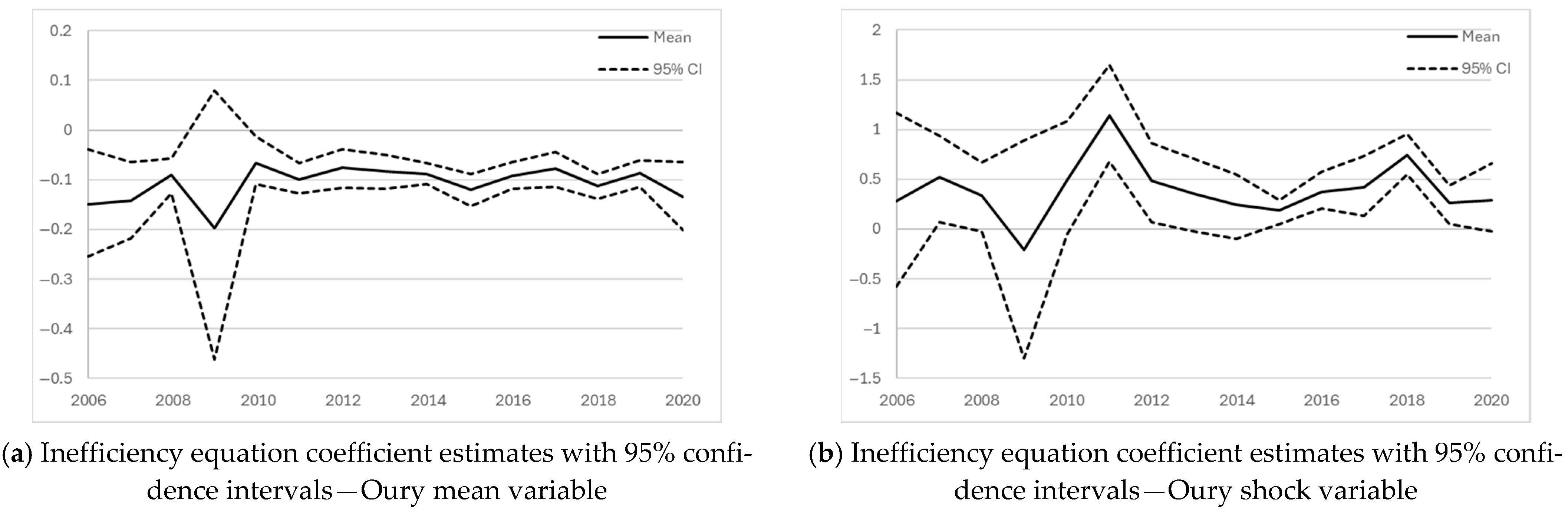
| Year. | Inefficiency Equation Based on Specification 3 | |||||||
|---|---|---|---|---|---|---|---|---|
| Oury Mean Coefficient | std. err. | t-Ratio | Oury Shock Coefficient | std. err. | t-Ratio | |||
| 2006 | −0.149 | 0.057 | −2.63 | *** | 0.280 | 0.441 | 0.63 | |
| 2007 | −0.143 | 0.041 | −3.51 | *** | 0.512 | 0.217 | 2.35 | *** |
| 2008 | −0.090 | 0.017 | −5.32 | *** | 0.324 | 0.180 | 1.81 | * |
| 2009 | −0.197 | 0.145 | −1.36 | −0.225 | 0.567 | −0.40 | ||
| 2010 | −0.066 | 0.025 | −2.65 | *** | 0.512 | 0.279 | 1.84 | * |
| 2011 | −0.099 | 0.015 | −6.59 | *** | 1.167 | 0.246 | 4.74 | *** |
| 2012 | −0.076 | 0.021 | −3.59 | *** | 0.448 | 0.198 | 2.26 | ** |
| 2013 | −0.083 | 0.017 | −4.96 | *** | 0.336 | 0.185 | 1.82 | * |
| 2014 | −0.089 | 0.012 | −7.40 | *** | 0.224 | 0.172 | 1.31 | |
| 2015 | −0.120 | 0.016 | −7.68 | *** | 0.154 | 0.064 | 2.41 | *** |
| 2016 | −0.092 | 0.013 | −7.16 | *** | 0.387 | 0.094 | 4.12 | *** |
| 2017 | −0.077 | 0.019 | −4.03 | *** | 0.416 | 0.159 | 2.61 | *** |
| 2018 | −0.113 | 0.013 | −8.47 | *** | 0.738 | 0.101 | 7.32 | *** |
| 2019 | −0.086 | 0.014 | −6.23 | *** | 0.224 | 0.110 | 2.04 | ** |
| 2020 | −0.135 | 0.035 | −3.82 | *** | 0.284 | 0.170 | 1.68 | * |
| (1) | (2) | (3) | (4) | (5) | (6) | |
|---|---|---|---|---|---|---|
| Variables | TE | CTE | TE North | CTE North | TE South | CTE South |
| Yield Monitors | 0.0046 | 0.014 *** | −0.029 *** | −0.0033 | 0.0093 * | 0.016 *** |
| (0.91) | (2.74) | (−3.04) | (−0.46) | (1.65) | (2.81) | |
| Variable Rate Technology | −0.0025 | 0.0013 | −0.013 ** | −0.0048 | −0.0036 | −0.0073 |
| (−0.46) | (0.28) | (−2.37) | (−1.04) | (−0.43) | (−1.05) | |
| Field Insurance | −0.0033 | 0.0025 | 0.014 | −0.0019 | −0.012 | −0.0075 |
| (−0.50) | (0.40) | (1.23) | (−0.25) | (−1.61) | (−1.06) | |
| Farmer Experience | −0.029 ** | −0.013 | −0.021 | 0.0012 | −0.026 * | −0.019 |
| (−2.09) | (−0.94) | (−0.80) | (0.058) | (−1.80) | (−1.28) | |
| Cover Cropping | 0.0012 | 0.0023 | −0.00074 | −0.0012 | 0.0011 | 0.0060 ** |
| (0.66) | (1.32) | (−0.30) | (−0.60) | (0.43) | (2.53) | |
| Fallow Periods | 0.013 * | 0.034 *** | 0.0082 | 0.014 * | 0.013 | 0.064 *** |
| (1.95) | (3.89) | (0.88) | (1.68) | (0.91) | (4.76) | |
| Conservation Tillage | 0.0034 | 0.011 *** | 0.0011 | 0.010 *** | 0.0073 ** | 0.012 *** |
| (1.60) | (5.47) | (0.29) | (2.72) | (2.36) | (5.01) | |
| Replanted Acreage | −0.0040 * | −0.017 *** | 0.0027 | −0.0070 *** | −0.012 *** | −0.025 *** |
| (−1.71) | (−6.94) | (0.81) | (−2.95) | (−2.90) | (−7.40) | |
| Land Rent | 0.0052 | 0.0074 | −0.0099 | 0.013 * | 0.031 *** | 0.028 *** |
| (0.85) | (1.41) | (−1.05) | (1.91) | (3.23) | (3.43) | |
| Improved Tile Drainage | −0.0030 | 0.0069 *** | 0.0050 | 0.0088 *** | −0.0088 * | 0.0052 |
| (−1.28) | (2.75) | (1.55) | (4.04) | (−1.75) | (1.05) | |
| Irrigated Acreage | −0.0047 *** | 0.00037 | 0.0011 | 0.0033 *** | −0.010 *** | −0.0080 *** |
| (−3.72) | (0.27) | (0.63) | (2.68) | (−3.79) | (−2.95) | |
| Grass Waterways | 0.00015 | 0.0027 | 0.0078 * | 0.00089 | −0.00074 | −0.0040 |
| (0.065) | (1.21) | (1.75) | (0.28) | (−0.25) | (−1.25) | |
| Contour Farming | −0.0039 ** | 0.0049 *** | −0.0045 * | 0.0076 *** | −0.0016 | 0.0077 *** |
| (−2.46) | (3.03) | (−1.85) | (3.33) | (−0.75) | (3.43) | |
| Terraces | 0.0016 | 2.69 × 10⁻⁶ | −0.0042 ** | −0.0056 *** | −0.00047 | −0.0020 |
| (0.95) | (0.0018) | (−1.98) | (−2.60) | (−0.17) | (−0.91) | |
| Constant | 0.67 | 0.53 | 0.80 | 0.63 | 0.57 | 0.49 |
| (9.43) | (7.00) | (6.35) | (8.26) | (6.09) | (5.06) | |
| Observations | 481 | 481 | 195 | 195 | 286 | 286 |
| R2 | 0.593 | 0.875 | 0.758 | 0.893 | 0.541 | 0.872 |
Disclaimer/Publisher’s Note: The statements, opinions and data contained in all publications are solely those of the individual author(s) and contributor(s) and not of MDPI and/or the editor(s). MDPI and/or the editor(s) disclaim responsibility for any injury to people or property resulting from any ideas, methods, instructions or products referred to in the content. |
© 2025 by the authors. Licensee MDPI, Basel, Switzerland. This article is an open access article distributed under the terms and conditions of the Creative Commons Attribution (CC BY) license (https://creativecommons.org/licenses/by/4.0/).
Share and Cite
Wang, S.L.; Olver, R.; Bonin, D. Sustainable Crop Farm Productivity: Weather Effects, Technology Adoption, and Farm Management. Sustainability 2025, 17, 6778. https://doi.org/10.3390/su17156778
Wang SL, Olver R, Bonin D. Sustainable Crop Farm Productivity: Weather Effects, Technology Adoption, and Farm Management. Sustainability. 2025; 17(15):6778. https://doi.org/10.3390/su17156778
Chicago/Turabian StyleWang, Sun Ling, Ryan Olver, and Daniel Bonin. 2025. "Sustainable Crop Farm Productivity: Weather Effects, Technology Adoption, and Farm Management" Sustainability 17, no. 15: 6778. https://doi.org/10.3390/su17156778
APA StyleWang, S. L., Olver, R., & Bonin, D. (2025). Sustainable Crop Farm Productivity: Weather Effects, Technology Adoption, and Farm Management. Sustainability, 17(15), 6778. https://doi.org/10.3390/su17156778