Article

Spatiotemporal Dengue Forecasting for Sustainable Public Health in Bandung, Indonesia: A Comparative Study of Classical, Machine Learning, and Bayesian Models

by
I Gede Nyoman Mindra Jaya
1,*,
Yudhie Andriyana
1,
Bertho Tantular
1,
Sinta Septi Pangastuti
1 and
Farah Kristiani
2
1
Department of Statistics, Universitas Padjadjaran, Sumedang 45363, Indonesia
2
Department of Mathematics, Parahyangan Catholic University, Kota Bandung 40141, Indonesia
*
Author to whom correspondence should be addressed.
Sustainability 2025, 17(15), 6777; https://doi.org/10.3390/su17156777
Submission received: 17 June 2025 / Revised: 19 July 2025 / Accepted: 22 July 2025 / Published: 25 July 2025
(This article belongs to the Section Health, Well-Being and Sustainability)

Abstract

Accurate dengue forecasting is essential for sustainable public health planning, especially in tropical regions where the disease remains a persistent threat. This study evaluates the predictive performance of seven modeling approaches—Seasonal Autoregressive Integrated Moving Average (SARIMA), Extreme Gradient Boosting (XGBoost), Recurrent Neural Network (RNN), Long Short-Term Memory (LSTM), Bidirectional LSTM (BiLSTM), Convolutional LSTM (CNN–LSTM), and a Bayesian spatiotemporal model—using monthly dengue incidence data from 2009 to 2023 in Bandung City, Indonesia. Model performance was assessed using MAE, sMAPE, RMSE, and Pearson’s correlation (R). Among all models, the Bayesian spatiotemporal model achieved the best performance, with the lowest MAE (5.543), sMAPE (62.137), and RMSE (7.482), and the highest R (0.723). While SARIMA and XGBoost showed signs of overfitting, the Bayesian model not only delivered more accurate forecasts but also produced spatial risk estimates and identified high-risk hotspots via exceedance probabilities. These features make it particularly valuable for developing early warning systems and guiding targeted public health interventions, supporting the broader goals of sustainable disease management.

1. Introduction

Sustainable public health is a core focus of Sustainable Development Goal 3, which aims to “ensure healthy lives and promote well-being for all at all ages.” One way to achieve sustainable public health is by controlling the spread of disease in a sustainable manner.
Infectious diseases continue to exert a profound impact on global health and economic stability. The COVID–19 pandemic underscored how rapidly an infectious disease can disrupt societies and economies worldwide [1]. Among vector-borne diseases, dengue persists as a major public health threat in tropical and subtropical regions, particularly in Indonesia [2]. Transmitted by Aedes aegypti mosquitoes, dengue causes substantial morbidity and mortality, especially in densely populated urban centers [3]. According to the WHO, it is estimated that globally, about 390 million individuals are infected with the dengue virus each year, of which approximately 96 million cases exhibit clinical symptoms [2,4].
Dengue has hit Indonesia hard; in 2023, there were more than 114,720 reported cases and 894 verified deaths [5]. Dengue has a big economic impact, with treatment costs ranging from USD 156 to USD 625 per patient every episode, depending on how bad the disease is [6]. This financial burden puts a lot of stress on both families and healthcare workers.
Bandung City, located in West Java, is one of the most significant areas for dengue in Indonesia. With a population of approximately 2.5 million, the city recorded an average dengue incidence rate of 136 cases per 100,000 people from 2009 to 2023, categorizing it as a high-risk area [7]. The Bandung City Health Office [7] records that there were 1865 documented cases of dengue in early 2023, which led to eight deaths. These patterns show how important it is to use data to stop future outbreaks and show that the number of cases is rising. To protect communities from dengue and lessen its wider economic effects, both the government and the public must work together to solve health problems associated to the disease. There are several things that make the dengue problem very complicated, like the weather, how people in the community live their lives, and efforts to manage the vectors. These factors significantly influence the fluctuations in dengue incidences over time and across different regions [8].
Early Warning Systems (EWSs) are an effective tool for disease management [9]. EWSs rely on accurate and timely forecasting models that can predict how and where diseases will spread over time and space. We have specified that our EWS is designed to forecast monthly dengue cases and their relative spatial risk. The spatiotemporal variation of dengue cases is influenced by many factors, including weather and sociodemographic conditions [8,10]. However, the effect of each variable often varies by study location because of the complex interactions among weather variables [8]. For forecasting—rather than causal inference—we developed a univariate forecasting model for the EWS, focusing only on the spatiotemporal variation of dengue cases. We argue that the effects of all relevant variables influencing dengue’s spatiotemporal dynamics are inherently captured within the dengue data itself and are accounted for through the spatiotemporal variation components. Furthermore, according to [11], a univariate model is more suitable for forecasting count data than a causal model because causal approaches may suffer from double-counting errors due to prediction uncertainty in exogenous variables that must also be forecasted. The forecasting model we developed provides information about high-risk areas, which can then be used to identify the main local drivers of dengue outbreaks. These models help public health authorities develop targeted vector control strategies, allocate resources more effectively, and take rapid action in high-risk areas. In this context, accurate spatiotemporal forecasting is critical [10]. Following previous studies [12], areas were classified as high risk if the total number of dengue cases exceeded the second quartile (Q2) threshold (classified as “High”) or the upper quartile (Q3) threshold (classified as “Very High”), or if the exceedance probability was greater than 80% for either level. In simple terms, this means an area is considered high risk when it has significantly more cases than most other areas.
Selecting an appropriate forecasting model is crucial for developing accurate and effective EWS [13]. Previous studies on dengue forecasting have employed a wide range of approaches, each with its own strengths and limitations. These include classical statistical models such as the Seasonal Autoregressive Integrated Moving Average (SARIMA) [14]; machine learning (ML) methods like Extreme Gradient Boosting (XGBoost) [15]; deep learning (DL) architectures such as Recurrent Neural Networks (RNN), Long Short–Term Memory (LSTM), and its variants—Bidirectional LSTM (BiLSTM) and Convolutional LSTM (CNN–LSTM) [16]—as well as Bayesian spatiotemporal models [13,17].
This study seeks to determine the most effective forecasting model for predicting dengue cases in Bandung, Indonesia. It is hypothesized that, despite the growing prominence of artificial intelligence and big data, Bayesian methods continue to offer significant value in epidemiological research due to their ability to incorporate uncertainty and complex spatiotemporal structures.
This paper is organized as follows: Section 2 provides an overview of forecasting approaches; Section 3 presents the application to monthly dengue incidence data in Bandung, Indonesia; Section 4 discusses the findings; and Section 5 concludes the study.

2. Overview of Forecasting Approaches

Classical approaches like SARIMA are well suited for univariate time series with clear seasonal patterns, offering simplicity and interpretability. However, they assume linearity and stationarity, and do not account for spatial dependencies [14]. ML methods like XGBoost provide strong predictive performance, particularly for nonlinear patterns, but they often struggle with long-term dependencies and lack spatial modeling capabilities [18,19]. DL architectures (RNNs, LSTMs, BiLSTM, CNN–LSTM) can effectively learn complex temporal patterns, with CNN–LSTM further capturing spatial structures. Yet, they require large datasets, are computationally intensive, and are often criticized for limited interpretability [16,20,21,22,23]. Bayesian spatiotemporal models offer a principled framework to capture both spatial and temporal heterogeneity, account for uncertainty, and support inference in data-scarce contexts. These models are highly interpretable and suitable for identifying high-risk areas and supporting public health interventions [24].
To enhance clarity and readability, Table 1 summarizes the key characteristics, strengths, and limitations of each forecasting approach evaluated in this study. Detailed model formulations and equations are provided in Appendix A.
To implement all forecasting models described in Table 1 for predicting dengue incidence, we present the model configurations and hyperparameter settings for classical, machine learning, deep learning, and Bayesian approaches in Table 2 below.
The column “Architecture/Structure” in Table 2 specifies each model’s internal configuration, such as neural network layers or classical or Bayesian models. The number of full runs across the training dataset during model learning is called “Training Epochs”. The number of data samples analyzed before updating the model’s internal parameters is called “Batch Size”. “Optimizer/Learning Rate” lists the optimization technique (e.g., Adam, XGBoost) used to minimize model error and the learning rate that determines update step size. “Regularization Method” includes dropout in deep learning and priors in Bayesian models to prevent overfitting. Finally, “Description/Notes” describes input types, feature engineering, and implementation details in the model. N/A denotes that the mean is not defined for this model. To evaluate the predictive accuracy and goodness-of-fit of the proposed models, we employed several commonly used metrics, including Mean Absolute Error (MAE), Root Mean Squared Error (RMSE), and Pearson’s correlation coefficient (R). Detailed formulations of these metrics are provided in Appendix A.

3. Application: Monthly Dengue Incidences in Bandung, Indonesia
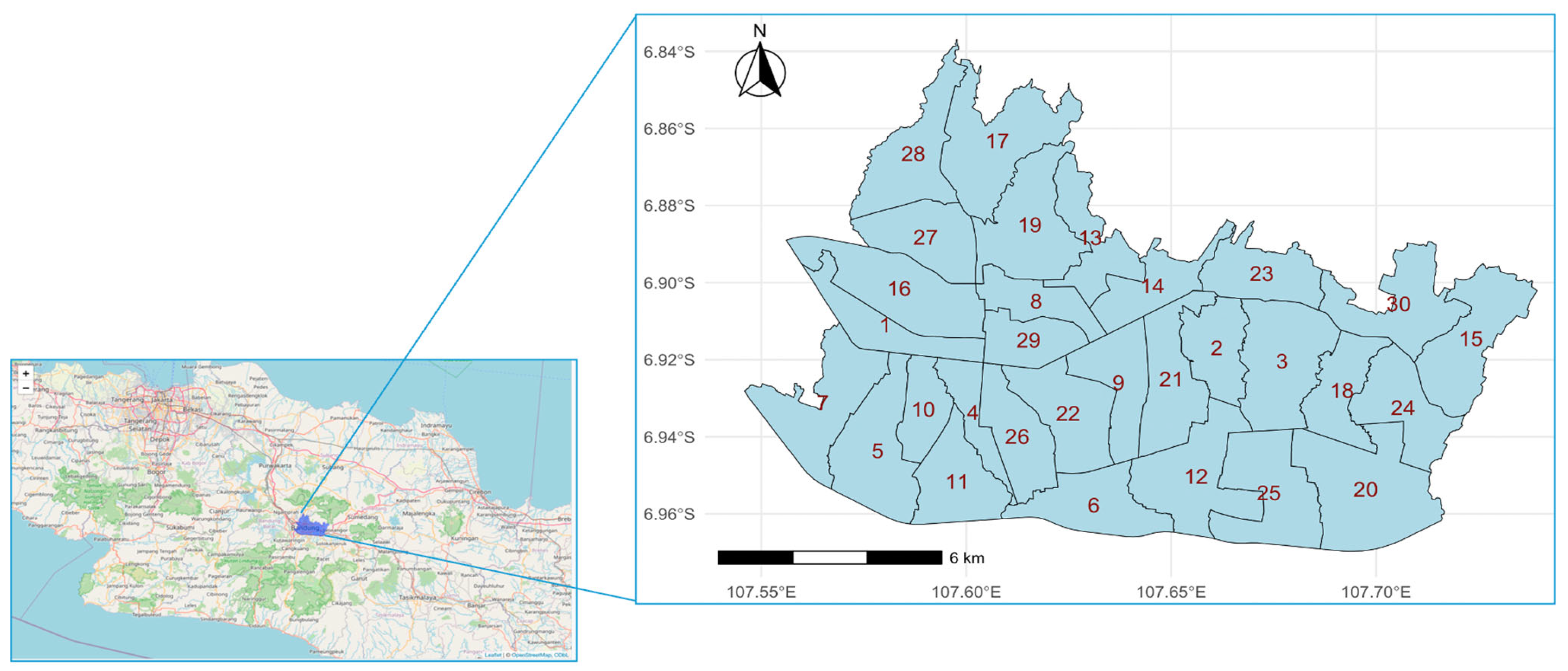
3.1. Study Area

Bandung City (Figure 1) is located in West Java Province, covering an area of 167.31 km2. In 2024, the city recorded a population of 2,591,763 with a population density of approximately 15,000 inhabitants per km2. As a highly dense and mobile urban center, Bandung presents a substantial risk for the transmission of infectious diseases, including dengue. Geographically, much of Bandung lies in highland areas with relatively high rainfall, creating favorable conditions for the proliferation of disease vectors such as Aedes aegypti mosquitoes. According to the West Java Provincial Health Office, Bandung consistently reports the highest number of cases in the West Java province each year.

3.2. Data

In this study, dengue case data were obtained through an active surveillance system, ensuring that the reported figures reflect direct monitoring by health officers. The data, collected by the Bandung City Health Office from 2009 to 2023, recorded a total of 58,126 dengue cases across 30 districts over a 15-year period—averaging approximately 3875 cases per year. The highest total number of incidents was reported in 2009 with 6678 cases, whereas the lowest level was observed in 2017 with 1786 cases. In general, dengue incidence tends to peak early in the year, particularly in January, with the detailed distribution presented in Table 3 and Figure 2.
Table 3 presents a descriptive summary of the monthly distribution of dengue cases across 30 districts in Bandung City from 2009 to 2023. Each month consistently shows a minimum value of zero, recorded across different years, indicating that certain districts reported no dengue cases in specific months. This highlights notable spatial and temporal variability in disease occurrence. While zero values could suggest potential underreporting, the data were obtained through an active surveillance system managed by the Bandung City Health Office. This systematic approach reduces the likelihood of undetected cases, allowing the zero values to be interpreted as genuine absences of reported infections rather than data gaps. On average, monthly dengue cases ranged between 7 and 13, with median values from 6 to 9. The boxplots in Table 2 also show that the highest concentrations of cases generally occurred in the earlier months of the year, particularly between January and June. These findings emphasize the substantial variation in dengue incidence across both time and geography, reinforcing the need for spatiotemporal modeling approaches.
Below, we present the monthly spatial distribution of total dengue cases across 30 districts from 2009 to 2023.
The color categories in Figure 2 are based on quartile ranges: Very Low (<Q1), Low (Q1–Q2), High (Q2–Q3), and Very High (>Q3). Based on Figure 2, it can generally be observed that dengue cases tend to be higher in several districts during the early months of the year, particularly from January to June. Additionally, there appears to be a spatial concentration of cases in the northern and central parts of Bandung City.

3.3. Model Estimation

As previously discussed, developing an Early Warning System (EWS) critically depends on the ability to accurately forecast dengue case counts in upcoming years. Accurate forecasting enables governments with limited resources to focus intervention efforts on districts predicted to have high case burdens. For this purpose, the research explores a selection of predictive models, including classical time series, ML, DL, and Bayesian approaches. Each model has undergone performance evaluation to ensure that the selected configuration represents the best-performing combination of parameters. For example, the optimal configuration for the LSTM model consists of LSTM (64) → Dropout (0.3) → Dense (1), with 100 epochs, dropout regularization of 0.3, a learning rate of 0.001, and a supervised sequence length of 12 time steps. The best-performing parameters for all models are summarized in Table 3.
In this model estimation, we utilize spatiotemporal data covering 30 districts over a 15-year period, resulting in 180 monthly time points. This yields a total of 5400 observations (30 × 180), providing a sufficiently large dataset to ensure statistically robust results. To identify the best-performing forecasting model, we employ both in-sample and out-of-sample evaluation approaches. Data from 2009 to 2021 (4680 observations) is used for training, while data from 2022 to 2023 (720 observations) is reserved for testing. This corresponds to approximately 86% of the data for training and 14% for testing. As suggested by [26], a minimum of 10% test data is generally adequate for model evaluation. The two-year testing period is chosen to enable the model to learn from an extended historical sequence and to match the forecasting objective of predicting dengue cases for the upcoming two years, 2024 and 2025.

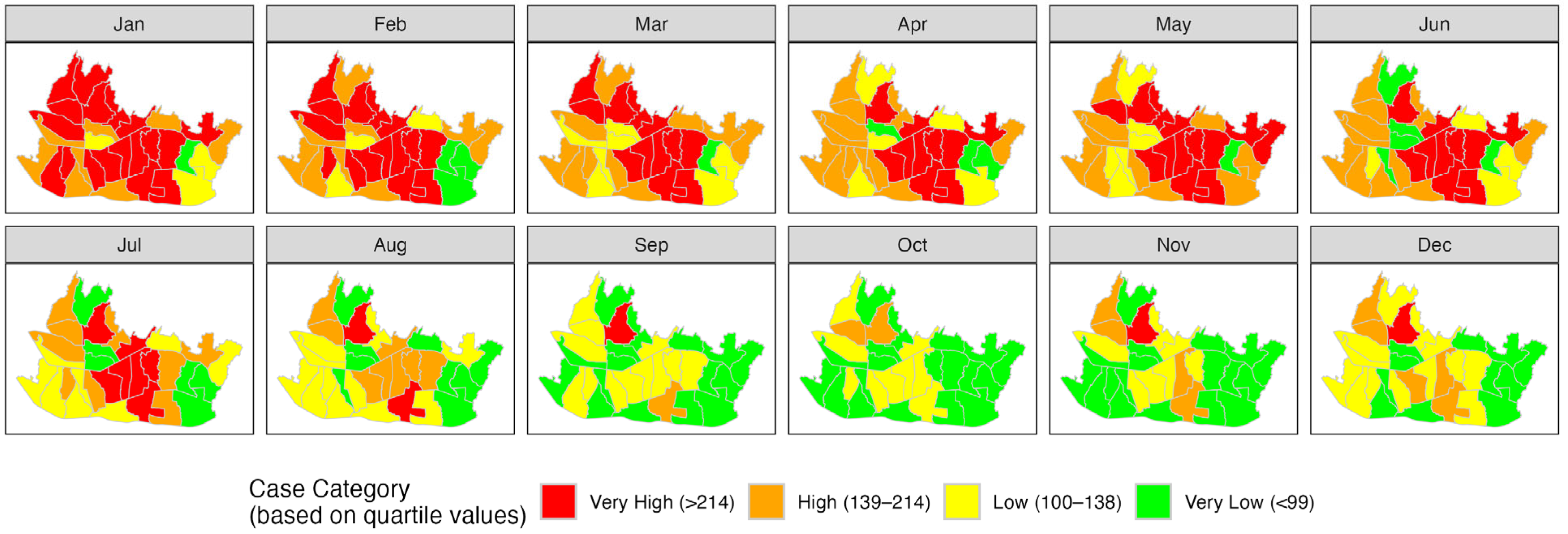
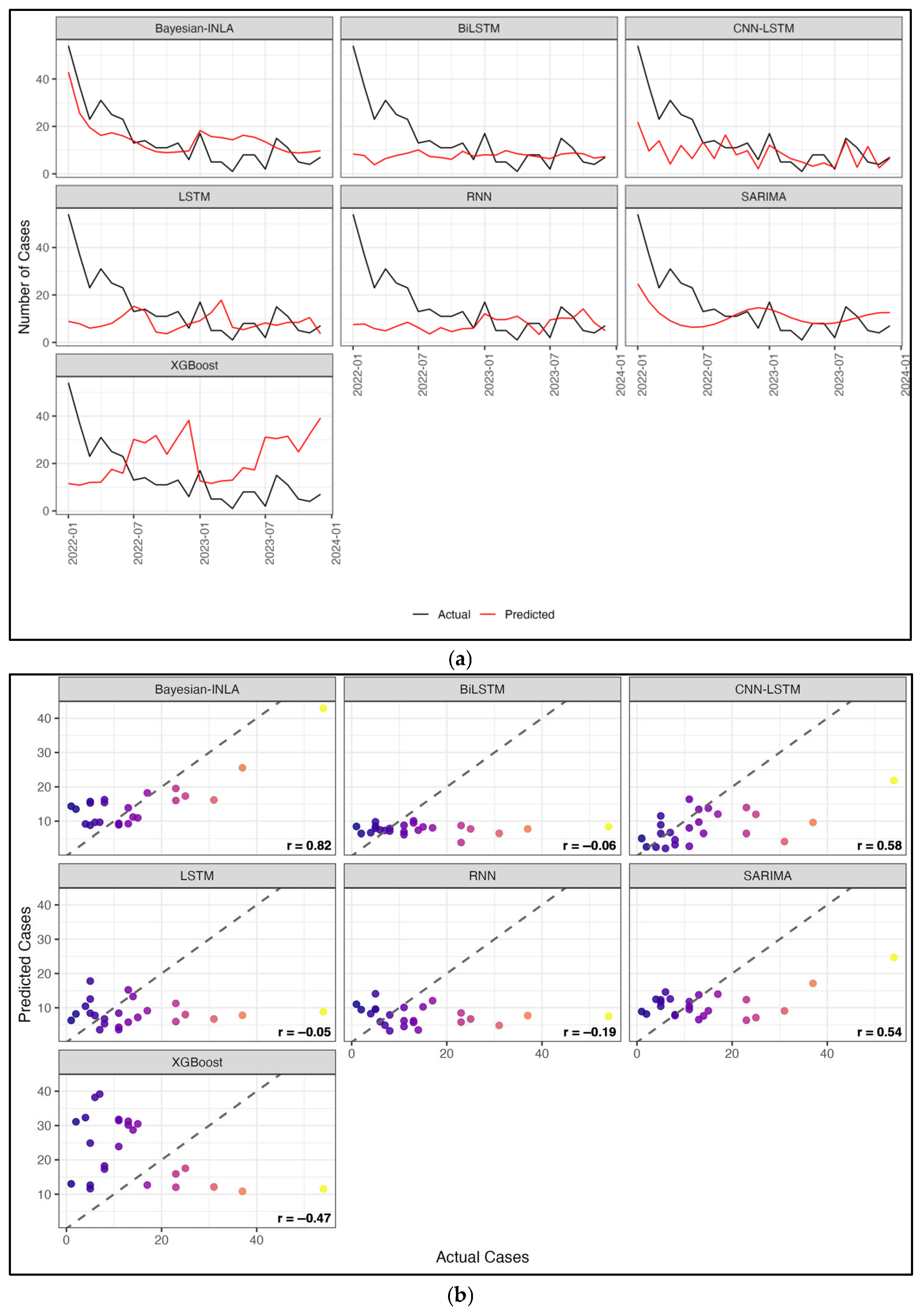
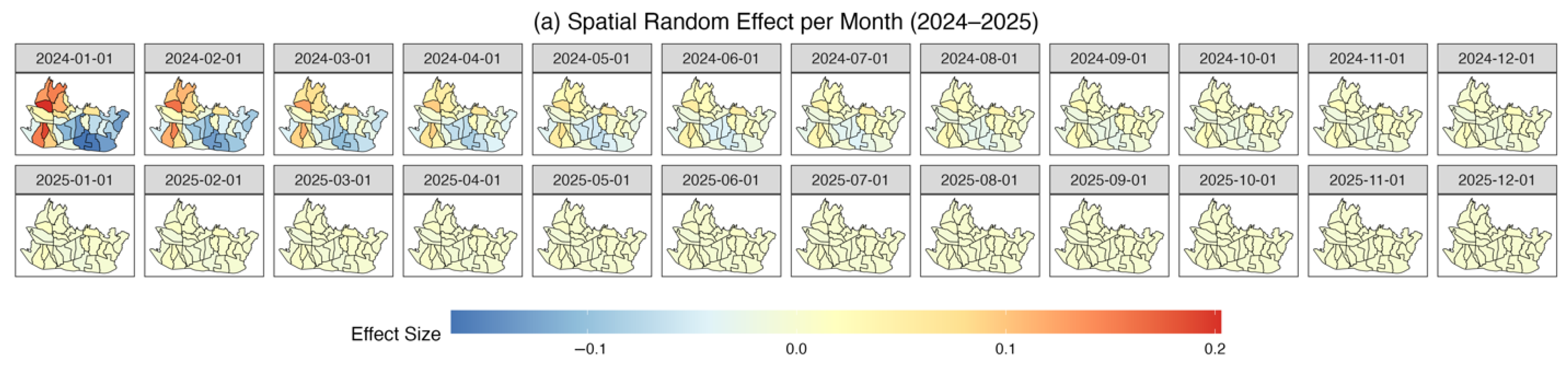
3.4. Result and Model Comparison

To identify the best forecasting model for dengue cases, a comparison was conducted between several models: SARIMA, XGBoost, RNN, LSTM, BiLSTM, CNN–LSTM, and a Bayesian spatiotemporal model. The evaluation was based on multiple metrics, including Mean Absolute Error (MAE), symmetric Mean Prediction Error (sMAPE), Root Mean Square Error (RMSE), and Pearson’s correlation (R). A good forecasting model is characterized by low MAE, sMAPE, and RMSE values and a high correlation value between predicted and actual cases. Each model was assessed using two data groups: training data and testing data. The purpose was to determine whether a model performs well both during training and testing, or if it only shows excellent performance during training but performs poorly during testing, which could indicate overfitting. Table 4 displays the results of the model comparison.
The main finding of this analysis is that the XGBoost model demonstrates outstanding forecasting performance on the training dataset but performs poorly on the testing dataset, indicating a high risk of overfitting. In contrast, the SARIMA model shows reasonably good and balanced performance across both datasets, although it still falls short compared with the Bayesian spatiotemporal model. The RNN, Bi–LSTM, and CNN–LSTM also failed to deliver satisfactory forecasts. This may be due to the relatively limited temporal data used in the training phase—only 12 months across 13 years—which might not be sufficient for DL models to learn complex patterns. Moreover, these models may struggle to adequately model the temporal and spatial dependencies embedded in the data. Overall, the Bayesian spatiotemporal model emerged as the best-performing model, with consistently strong results on both training and testing datasets. While it did not outperform XGBoost on the training data alone, its balanced and robust performance suggests that it is less prone to overfitting. This advantage likely stems from the Bayesian model’s capability to effectively handle relatively small datasets and to capture the spatiotemporal pattern and interactions in the data. To facilitate a clear comparison between model predictions and actual data during the 2022–2023 testing period, and to evaluate the performance of each forecasting model, we present the results for the Antapani district as an illustrative example (Figure 3). Visualizing all 30 districts in detail would not be practical, so Antapani was selected solely because it appears first in the sequential list of districts. Figure 3 demonstrates that the Bayesian–INLA model provides a better fit between the observed and predicted values compared with the other models.
Model evaluation should not rely solely on aggregate accuracy metrics across all spatiotemporal units. A more insightful approach involves examining the temporal pattern alignment between predicted and observed (testing) data at the district level for each forecasting model. To support this type of analysis, we developed an Interactive Dashboard for Dengue Case Prediction, as illustrated in Figure 4. This dashboard allows users to explore temporal trends of predicted versus observed cases across districts, prediction models, and forecast periods. In addition to time series visualizations, the dashboard provides spatiotemporal maps that display the distribution of predicted case counts, relative risk, and identified hotspots. Its dynamic and user-friendly interface facilitates a more nuanced interpretation of model performance, helping users to determine the most effective forecasting method for dengue cases—particularly in the context of Bandung City. The dashboard is publicly accessible at https:/diseasemodel.shinyapps.io/rshinyapp/, accessed on 5 May 2025.
Table 5 presents the estimated fixed parameters of the spatiotemporal regression model in Equation (A12). The model is estimated under the assumption that the data follow a negative binomial distribution due to the presence of overdispersion, with a dispersion parameter of 12.74 (Table 6). The estimated coefficient for the time trend (β) is −0.040 with a 95% credible interval ranging from −0.071 to −0.010, suggesting a statistically significant downward trend in dengue incidence over time. This corresponds to an approximate 4% annual decrease in case numbers. However, despite this declining trend, the total number of cases remains relatively high, with over 2000 cases reported each year on average.
Table 6 and Figure 5 demonstrate that the temporal random effects are the most significant variables explaining the spatiotemporal variations in relative dengue risk—particularly the seasonal and AR2 components for monthly data, which together account for a total variance of 29.36%. In addition, the AR2 structure for yearly data contributes significantly with a total variance of 24.80%, followed by the heterogeneity component (23.96%). The interaction between space and time also plays a notable role, contributing 19.21% to the total variance. Based on the fixed and random components, we derived the forecast of dengue cases. These forecasts are visualized through a line chart in Figure 6 and spatial maps in Figure 7: Figure 7a presents the predicted number of dengue cases, Figure 7b shows the corresponding relative risk, and Figure 7c illustrates the exceedance probabilities.
Figure 6 and Figure 7 demonstrate that the anticipated number of cases, relative risk, and exceedance probability typically reach their maximum in the initial months of the year. The number of predicted dengue incidences is relatively high across most districts in January and February, decreases slightly in March and April, rises again in May and June, and then gradually declines from July through December. Notably, some districts still report over 20 cases during July and August. Relative risk patterns follow a similar trend: high risk is observed in January and February, followed by a decline in March–April, a resurgence in May–June, and then a steady decrease until the end of the year.

4. Discussion

Accurate forecasting of dengue incidence is critical to the development of Early Warning Systems (EWS), which enable timely interventions and efficient allocation of health resources—key pillars of sustainable public health [27]. EWS depend on robust forecasting models that can predict when and where outbreaks are likely to occur. However, modeling dengue remains complex, particularly in developing countries, due to challenges such as incomplete data on key determinants, limited surveillance coverage, and the nonlinear and stochastic nature of disease transmission [8,13].
Although many studies have incorporated meteorological (e.g., rainfall, temperature, humidity) and socioeconomic factors (e.g., larval-free index, healthy house index) as covariates [8,10,15,25,28], this study focused solely on spatiotemporal patterns of dengue cases. We developed a univariate spatiotemporal forecasting model aimed at producing reliable predictions for EWS. The exclusion of covariates was intentional, as their effects can vary across space and time, introducing risks of overfitting and double-counting. This simplification enhances generalizability in operational settings. Univariate forecasting models, especially in the Bayesian framework, are particularly well suited to capture spatial and temporal heterogeneity through structured dependencies [11]. Once hotspots and trends are identified, further causal analyses can be undertaken to investigate contextual drivers of disease risk.
This study provided a comparative evaluation of seven forecasting models—classical (SARIMA), machine learning (XGBoost), deep learning (RNN, LSTM, Bi–LSTM, CNN–LSTM), and Bayesian spatiotemporal models—using monthly dengue data from Bandung City (2009–2023). Performance was assessed using MAE, sMAPE, RMSE, and Pearson’s correlation coefficient.
The Bayesian spatiotemporal model consistently outperformed all other models, achieving the lowest prediction errors and highest correlation on the testing set. These results align with prior research [17,29,30,31] and underscore the model’s strength not only in predictive accuracy but also in generating spatial risk estimates and quantifying uncertainty through exceedance probabilities. Its ability to model complex spatial–temporal dependencies using random effects (e.g., Leroux CAR priors [32]) makes it highly suitable for public health forecasting. This approach has been widely applied in previous studies on dengue prediction [17,29,30,31], demonstrating its effectiveness in capturing spatial and temporal dependencies, which in turn enhances predictive performance.
In contrast, although SARIMA and XGBoost performed well during training, they experienced sharp declines in accuracy on the test set, indicating overfitting. This can be attributed to their inability to generalize beyond strong temporal autocorrelations in the training data. SARIMA captures linear and seasonal patterns, and XGBoost can model complex nonlinear relationships; however, both lack the capacity to incorporate spatial autocorrelation [14,33,34].
Deep learning models, including RNN, LSTM, Bi–LSTM, and CNN–LSTM, showed more stable performance between training and testing phases. Yet, they did not outperform the Bayesian model. Their limitations are likely due to the relatively small sample size—180 monthly time points per district—which may be insufficient for training deep neural architectures effectively. Moreover, standard RNN, LSTM, and Bi–LSTM are not designed for spatial modeling [35], and while CNN–LSTM introduces some spatial awareness through convolutional layers, it still cannot adapt to varying strengths of spatial dependency as effectively as Bayesian models with structured priors.
These findings reaffirm the relevance of Bayesian spatiotemporal models in modern epidemiological forecasting. Their interpretability, capacity to incorporate uncertainty, and superior performance under data constraints make them particularly valuable in low-resource contexts. Bayesian spatiotemporal models are great for predicting the spread of diseases because they may borrow strength from different places and times to deal with problems like not having enough data, underreporting, and missing values, which are common problems with public health surveillance data [13,32].
Further, our analysis for the 2024–2025 forecast period showed that high exceedance probabilities (0.75–0.90) were concentrated in January—coinciding with Indonesia’s rainy season—indicating a clear seasonal pattern in risk. This corresponds with optimal breeding conditions for Aedes aegypti, the primary dengue vector. Conversely, the dry season (August to December) showed lower risk levels [35].
Despite these strengths, the study has several limitations. First, although data were obtained from the Bandung City Health Office using active surveillance, underreporting or missing values may still be present in certain districts or periods. Second, the use of a univariate approach—while suitable for operational forecasting—limits exploration of the underlying causes of transmission. Although multivariate models may provide explanatory insights [36], they risk introducing complexity and overfitting, especially when the relationships between variables are context dependent.
Future research should focus on developing separate causal models to investigate how external factors such as climate, the environment, and socioeconomic indicators affect the number of dengue cases over time and space. These factors are not necessary for making predictions because their impacts can change depending on the situation and may not always be the same. However, it is still crucial to know how they affect certain areas to improve public health planning and guide targeted interventions. To avoid problems like double-counting and overfitting that might lower prediction performance, causation analyses should be made separately from forecasting models.

5. Conclusions

This study conducted a comprehensive analysis of forecasting models for predicting dengue cases in Bandung City, comparing traditional statistical methods, machine learning (ML), deep learning (DL), and Bayesian approaches. The goal was to identify the most effective method for generating accurate and actionable forecasts that support public health decision–making. Among all the models evaluated, the Bayesian spatiotemporal model demonstrated the highest overall performance. It not only delivered superior predictive accuracy but also provided interpretable outputs, such as spatial risk estimates and hotspot identification. These features are crucial for early detection and timely public health interventions, particularly in urban settings with limited resources. Given the ongoing threat of dengue and the need for efficient resource allocation, we strongly recommend the integration of Bayesian methods into the development of Early Warning Systems (EWSs) for vector-borne diseases. Their ability to quantify uncertainty and model complex spatial–temporal dependencies makes them especially valuable for sustainable public health planning. For future research, we recommend developing dedicated causal models to identify local contextual factors that significantly influence dengue transmission and intervention effectiveness.

Author Contributions

Idea formulation, I.G.N.M.J. and Y.A.; methodology, I.G.N.M.J., Y.A., B.T. and S.S.P.; theory, I.G.N.M.J., Y.A., B.T. and F.K.; algorithm design, B.T. and S.S.P.; result analysis, I.G.N.M.J. and F.K.; writing, I.G.N.M.J. and F.K.; reviewing the research, I.G.N.M.J. and Y.A.; supervision, Y.A.; project administration, S.S.P.; funding acquisition, F.K. All authors have read and agreed to the published version of the manuscript.

Funding

This study received funding from Padjadjaran University via the Directorate of Research, Community Service, and Innovation (Grant Number: 4582/UN6.D/PT.00/2025).

Institutional Review Board Statement

Not applicable.

Informed Consent Statement

Not applicable.

Data Availability Statement

The R-4.3.1 graphical user interface (GUI) tool employed in this study is open-source and can be accessed via https://www.r-project.org (accessed on 1 January 2025). The R scripts created for this research are also open-source, with the code publicly available at https://github.com/mindra-bit/Dengue_Forecasting (accessed on 5 March 2025). All datasets used in this analysis are provided within the same repository.

Acknowledgments

We gratefully acknowledge the invaluable support provided by the Rectors of Universitas Padjadjaran and Parahyangan Catholic University through their Research Grant Programs, which made a significant contribution to this study.

Conflicts of Interest

The authors declare no conflicts of interest.

Appendix A. Classical, Machine Learning, and Bayesian Forecasting Models

Appendix A.1. The Seasonal Autoregressive Integrated Moving Average (SARIMA)

SARIMA is a sophisticated method for analyzing and forecasting series of data characterized by distinct seasonal trends. It builds on the basic ARIMA (Autoregressive Integrated Moving Average) model by adding extra parts to deal with seasonality. SARIMA adds three seasonal hyperparameters— P ,   D , and Q—along with a seasonal periodicity parameter s . This changes the basic A R I M A ( p , d , q ) into S A R I M A ( p , d , q ) ( P , D , Q ) s . In the SARIMA S A R I M A ( p , d , q ) ( P , D , Q ) s model, there are seven parameters. The parameters P and Q correspond to the orders of the seasonal AR and MA components, respectively, while D refers to the number of seasonal differences required to achieve stationarity. Similarly, p and q denote the orders of the nonseasonal AR and MA terms, and d denotes the quantity of nonseasonal differentiation procedures required to attain stationarity. For an input time series y t , the conventional SARIMA model is written as [37]
Φ P B s ϕ p B 1 B d 1 B s D y t = Θ Q ( B s ) θ q ( B ) ε t
where Φ P B s is the seasonal autoregressive (SAR) part of the SARIMA model. It takes into consideration how prior observations affect the model at seasonal intervals (i.e., every s periods). ϕ p B , on the other hand, stands for the nonseasonal autoregressive (AR) component, which means that the series’ current value is affected by its past values up to lag p . The formula 1 B d stands for the nonseasonal differencing operator, which is used d times to get rid of trends and make the time series stationary. Similarly, 1 B s D is the seasonal differencing operator, which is used D times to get rid of seasonal effects in the data. On the right side of the equation, Θ Q ( B s ) stands for the seasonal moving average (SMA) part, which takes into account the effects of past seasonal shocks or errors. The θ q ( B ) stands for the nonseasonal moving average (MA) part, which shows how past non–seasonal errors affect the present value. The word ε t denotes ‘white noise,’ signifying a stochastic disturbance at time t that is presumed to be distributed normally having an average of zero and constant variance. The backshift operator, denoted as B , shifts the time series one period backward. For example, B y t = y t 1 [37]. When you use SARIMA modeling on spatiotemporal data, you usually assume that the spatial units are not related to each other. This means that the model is fitted independently for each unit.

Appendix A.2. Extreme Gradient Boosting (XGBoost)

XGBoost is a powerful and highly scalable ML method that enhances the conventional Gradient Boosting framework. XGBoost is engineered to provide superior predictive performance through an optimized tree-learning methodology and facilitates parallel and distributed computing, thereby enhancing model training efficiency. The algorithm constructs a series of decision trees sequentially, with each new tree designed to reduce the residual errors from the preceding model. XGBoost integrates L1 (Lasso) and L2 (Ridge) penalty terms as part of its regularization strategies, to mitigate overfitting and enhance model generalization, rendering it exceptionally appropriate for structured data challenges in classification and regression tasks [38,39]. At iteration h , XGBoost employs a regularized objective function defined as follows:
O b j ( h ) = i = 1 n l y i , y ^ i ( h 1 ) + f h x i + Ω ( f h )
where l . represents a convex and differentiable loss function, such as squared error loss; y ^ i ( h 1 ) refers to the predicted value for sample i from the previous iteration; f h represents the decision tree model introduced in the current iteration h ; and Ω ( f h ) indicates the regularization component designed to control model complexity and reduce overfitting. The cumulative prediction for the ith sample after h repetitions is computed as
y ^ i ( h ) = i = 1 h f k x i = y ^ i ( h 1 ) + f h x i
This formulation demonstrates the forecasting process, in which each subsequent model incrementally improves upon the forecasts of the prior stage. Similar to SARIMA, XGBoost modeling is generally executed in a segmented approach, with the model being independently fitted for each spatial unit.

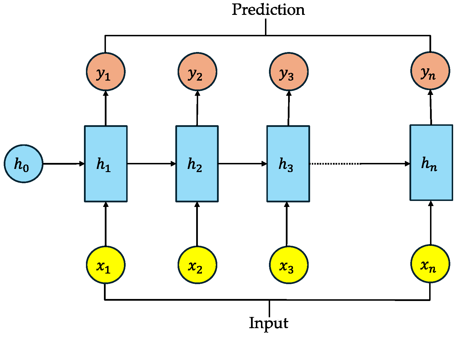
Appendix A.3. Recurrent Neural Networks (RNNs)

In the era of artificial intelligence, Recurrent Neural Networks (RNNs) have become one of the key neural network approaches for modeling sequential data, especially for data characterized by short-term dependency patterns [19,40]. RNNs belong to a unique group of artificial neural networks that are purpose-built to identify patterns in time series and various sequential data structures [41]. At every step t , the network receives x t as an input vector and updates h t hidden state in accordance with the following recurrent relation [40]:
h t = σ h W x h x t + W h h h t 1 + b h
where W x h denotes the weight matrix linking the x t to the h t , W h h represents the weight for hidden-to-hidden connections, b h is the bias vector, and σ h denotes the activation function. It is typically the hyperbolic tangent. The output at every time interval t is then calculated like this:
y t = σ y W h y h t + b y
where W h y represents the weight linking the hidden layer ( h t ) to the output layer ( y t ), b y is the corresponding bias, and σ y represents the activation function applied at the output layer.
Figure A1. Fundamental structure of an RNN. Adapted with permission from Ref. [40].
Sustainability 17 06777 g0a1
While RNNs are somewhat proficient in managing time series data, they are inadequate for capturing dependence over time because of the vanishing gradient issue. In RNNs, training is performed using the backpropagation method, where the error gradients are repeatedly computed and propagated backward through each previous time step. As the time steps become more distant, the gradient values—typically less than one—shrink further with each multiplication, which hampers the network’s ability to capture long-term dependencies [19].

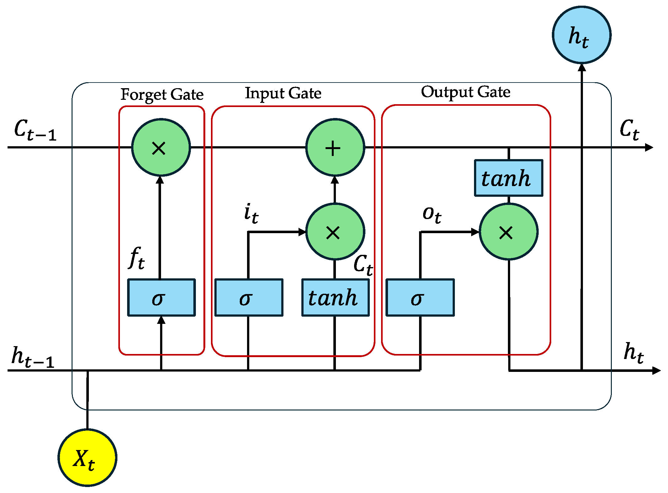
Appendix A.4. Long Short-Term Memory (LSTM)

LSTM architectures were introduced to address the vanishing gradient problem frequently encountered in RNNs. The LSTM architecture incorporates gating mechanisms to manage gradient flow, thereby overcoming the vanishing gradient issue and enabling the network to capture long-term dependencies. Figure A2 shows what the architecture looks like [40,42].
Figure A2. Fundamental architecture of an LSTM. Adapted with permission from Ref. [40].
Sustainability 17 06777 g0a2
An important innovation in LSTM networks is the use of gates to control the movement of information within the network. The presence of these gates enables LSTM cells to retain and update their memory over extended sequences, which helps them model long-term dependencies more successfully than standard RNNs. Every LSTM cell is equipped with three distinct gates: input, forget, and output. Collectively, these gates control the cell state ( c t ) and hidden state ( h t ), dictating the information to be retained, the data to be deleted, and the internal information to be transmitted to the subsequent layer or time step [40]. The equations for updating LSTM states are given below:
i t = σ W x i x t + W h i h t 1 + b i , f t = σ W x f x t + W h f h t 1 + b f , o t = σ W x 0 x t + W h 0 h t 1 + b 0 , g t = t a n h W x g x t + W h g h t 1 + b g , c t = f t c t 1 + i t g t , h t = o t tanh o t ,
where i t , f t , and o t denote the input gate, forget gate, and output gate, respectively, whereas g t signifies the candidate cell input. The variable c t represents the cell state, while h t corresponds to the hidden state. The LSTM process involves the utilization of many activation functions, such as the sigmoid σ . and t a n h ( . ) activation functions. The ⊙ signifies Hadamard multiplication [40].

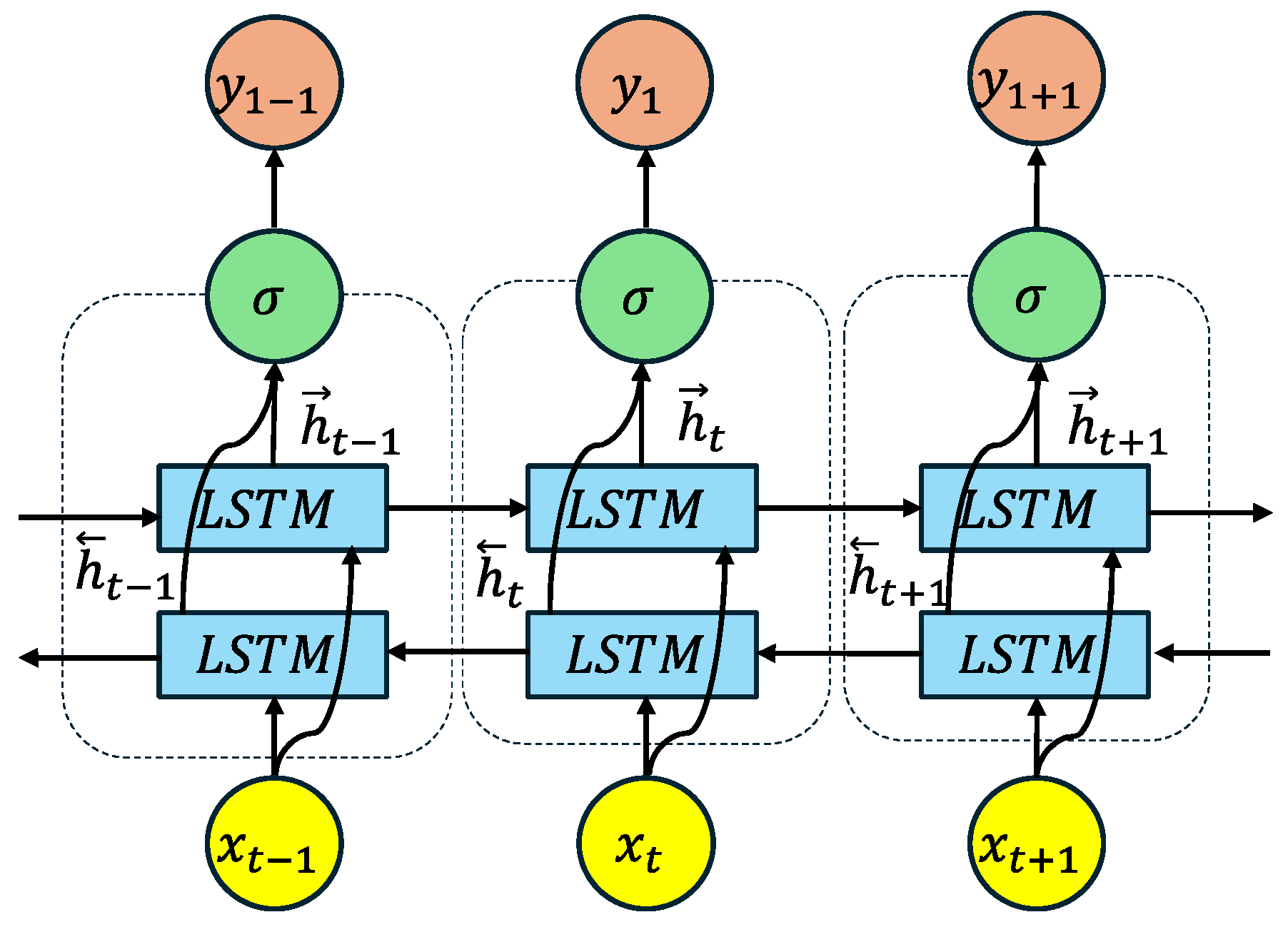
Appendix A.5. Bidirectional Long Short-Term Memory (BiLSTM)

As depicted in Figure A3, the BiLSTM architecture was developed to enhance the standard LSTM for time series data where patterns are strongly influenced by both long-term past values and subsequent conditions. The analysis of series data in both forward and backward orientations is how it accomplishes its objective. Through the utilization of this bidirectional computation, the model is able to utilize information from both the stages that came before and those that came after it, so enhancing its capability to learn dependencies that are long-term related. In a BiLSTM, each time step has two distinct hidden states: one from the forward pass ( h t ) and another from the backward pass ( h t ), as outlined in Equations (A7) and (A8).
h t = σ h W x h x t + W h h h t 1 + b h ,
h t = σ h W x h x t + W h h h t + b h ,
By integrating the hidden states generated in both forward and backward directions, the output y t is formed, as illustrated below:
y t = σ y W h y h t ; h t + b h ,
where [;] denotes concatenation. This architecture incorporates external recurrence across layers, simultaneously processing inputs in both forward and backward temporal directions while preserving separate hidden representations for each direction [42].
Figure A3. Fundamental architecture of BiLSTM. Adapted with permission from Ref. [40].
Sustainability 17 06777 g0a3

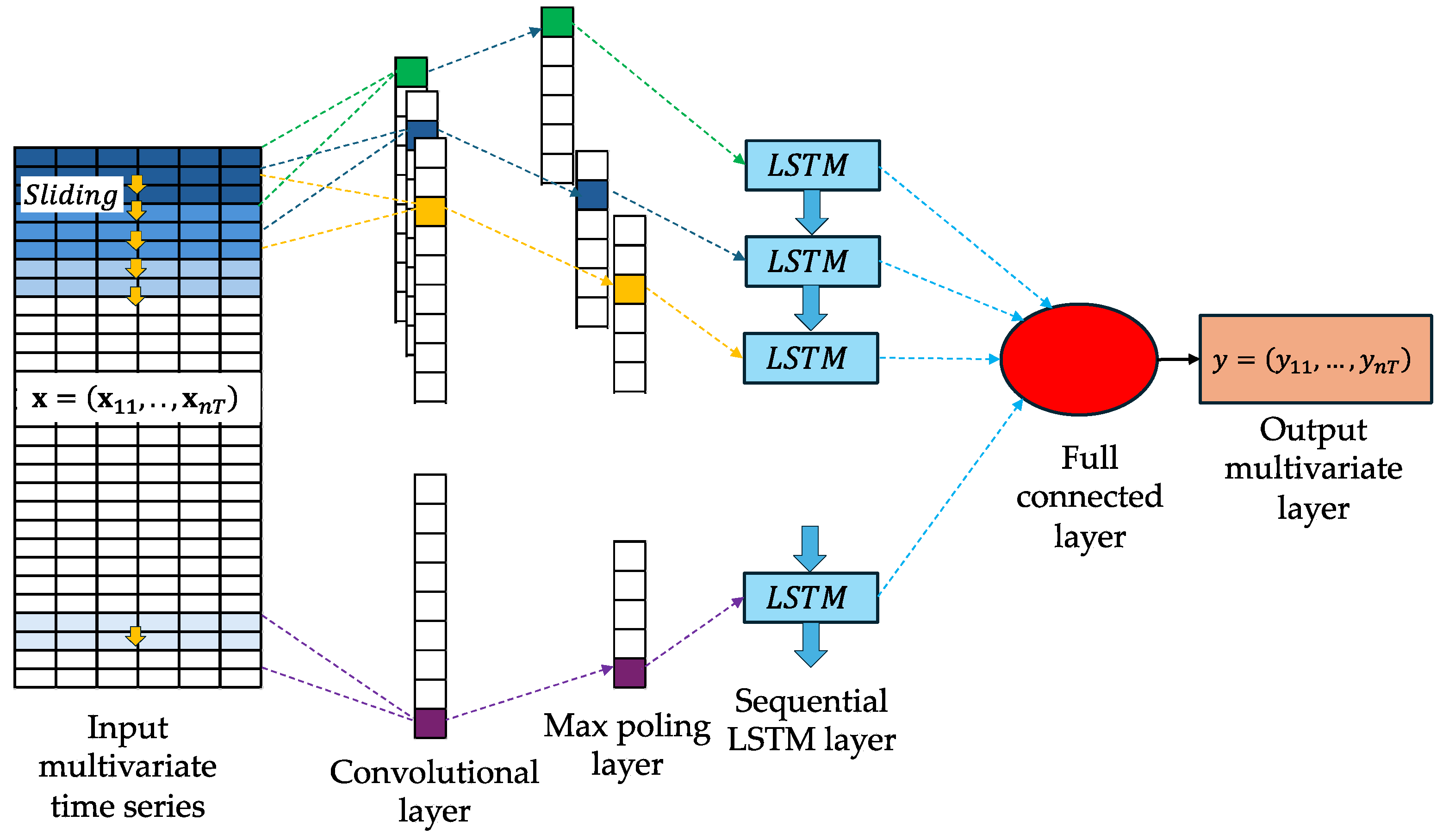
Appendix A.6. Convolutional Neural Network (CNN)

A CNN is an advanced form of Artificial Neural Network (ANN) specifically developed to handle visual data like images and videos, where recognizing spatial patterns is essential. Through the application of the CNN–LSTM, spatial features are extracted using CNNs and then modeled in sequence by LSTM. This combination makes CNN–LSTM especially effective for sequential prediction tasks involving spatial data, such as analyzing sequences of video frames or time-ordered images. Figure A4 below illustrates the architecture of the CNN–LSTM model [43,44]:
Figure A4. Fundamental architecture of CNN–LSTM. Adapted with permission from Ref. [43].
Sustainability 17 06777 g0a4

Appendix A.7. Bayesian Spatiotemporal

Assume that the random variable representing the number of cases in location i at time t , denoted as y i t , adheres to a Poisson distribution characterized by a rate parameter λ i t :
y i t | λ i t P o i s s o n λ i t ,   i = 1 , , n   a n d   t = 1 , , T ,
according to the log-linear predictor that was provided as:
log λ i t = α + x i t β + ω i + ν i + γ t + τ t + δ i t
where α denotes the intercept or the aggregate average number of cases across all districts and x i t β denotes the fixed effect component, which includes the linear trend. The symbols ω i and ν i denote the spatial dependency (structured random effect) and heterogeneity (unstructured random effect) of random components, respectively. Similarly, γ t and τ t represent the temporal dependency and heterogeneity random components, respectively. The interaction term δ i t encapsulates the integrated spatiotemporal dynamics. In the Bayesian paradigm, these components are treated as random variables assigned specific prior distributions. A Gaussian (normal) distribution prior with a mean of zero and a relatively large variation is assigned to the intercept α, which indicates that the prior is not one that provides any useful information. The spatial dependency effect ω i is represented by the Leroux Conditional Autoregressive (CAR) model, whereas ν i adheres to an exchangeable prior i i d N 0 , σ v 2 . The temporal dependency component γ t is represented by an autoregressive process of order p , while τ t is likewise presumed to adhere to an exchangeable prior. Ultimately, δ i t denotes the space–time interaction term, which can be delineated according to Type I–IV interaction frameworks, contingent upon the optimal model fit [32]. Please refer to Appendix B for detailed specifications of the prior distributions used for each model component. Note that, if overdispersion is present in the data, a negative binomial distribution will be used. The Bayesian spatiotemporal model is specified as follows:
log λ i t = α + β t y e a r + ν i + γ t m o n t h ( A R 2 ) + γ t m o n t h ( s e a s o n a l ) + γ t y e a r ( A R 2 ) + τ t m o n t h + τ t y e a r + δ i t
where α is the intercept capturing the overall level of relative risk, while β represents the slope of the annual time trend. The term ν i denotes the spatial heterogeneity random component. The components γ t and τ t capture both structured and unstructured temporal random effects, and δ i t accounts for the space–time interaction. The prior distributions assigned to each model parameter are summarized in Table A1.
Table A1. Explanation of the prior distributions for the parameters of the intercept, trend, and spatial, temporal, and space–time interaction effects of models (A12).
ComponentPrior
Intercept   ( α ) ~ i i d : α | σ α 2 ~ N 0 , σ α 2
Slope   ( β ) ~ i i d : β | σ β 2 ~ N 0 , σ β 2  
Spatially   unstructured   ( ν i ) ~ i i d : ν i | σ ν 2 ~ N 0 , σ ν 2
Temporally   structured   effect   ( γ t m o n t h ( A R 2 ) ) ~ A R ( 2 ) : γ t + 2 m o n t h ρ 1 m o n t h γ t + 1 m o n t h ρ 2 m o n t h γ t m o n t h | σ γ m o n t h 2 A R 2 ~ N 0 , σ γ m o n t h 2 A R 2 ;   i
Temporally   structured   effect   ( γ t m o n t h ( s e a s o n a l ) ) ~ S e a s o n a l ( 12 ) : γ t m o n t h + γ t + 1 m o n t h + + γ t + 11 m o n t h | σ γ 2 s e a s o n a l ~ N 0 , σ γ m o n t h 2 s e a s o n a l ;   i  
Temporally   structured   effect   ( γ t y e a r ( A R 2 ) ) ~ A R ( 2 ) : γ t + 2 y e a r ρ 1 y e a r γ t + 1 y e a r ρ 2 y e a r γ t y e a r | σ γ y e a r 2 A R 2 ~ N 0 , σ γ y e a r 2 A R 2 ;   i
Temporally   unstructured   effect   ( τ t m o n t h ) ~ i i d : τ t m o n t h | σ τ m o n t h 2 ~ N 0 , σ τ m o n t h 2
Temporally   unstructured   effect   ( τ t y e a r ) ~ i i d : τ t y e a r | σ τ y e a r 2 ~ N 0 , σ τ y e a r 2
Interaction effect~Type IV: Type   IV   integrates   both   the   spatially   structured   component   ( ω i )   and   the   temporally   structured   main   effect   ( γ t m o n t h ( A R 2 ) ) ,   suggesting   that   δ = δ 11 , , δ n T i = 1 ,   ,   n   a n d   t = 1 , , T is contingent upon in both spatial and temporal dimensions. The spatially structured effect follows Leroux CAR model: ω i | ω i , σ ω 2 , W ~ N ρ ω j = 1 n w i j ω j ρ ω i = 1 n w i j + 1 ρ ω , σ ω 2 ρ ω i = 1 n w i j + 1 ρ ω   t
with   W denotes an ( n × n ) the   first - order   queen   proximity   spatially   weights   matrix ,   in   which   w i j = 1   if   regions   i   and   j   share   a   common   boundary   or   vertex   ( i . e . ,   are   neighbors   under   the   queen   criterion ) ,   and   w i j = 1 otherwise.
The temporally structure is defined as follows:
γ ~ t + 2 m o n t h ρ ~ 1 m o n t h γ ~ t + 1 m o n t h ρ ~ 2 m o n t h γ ~ t m o n t h | σ ~ γ m o n t h 2 A R 2 ~ N 0 , σ ~ γ m o n t h 2 A R 2 ;   i
We adopted the Leroux Conditional Autoregressive (LCAR) prior to model spatial dependencies, as it explicitly distinguishes between structured and unstructured spatial variation—resolving identifiability issues inherent in traditional CAR formulations. Moreover, the LCAR prior offers greater flexibility in capturing varying levels of spatial autocorrelation, making it well suited for complex spatial structures [31]. For temporal dependencies, we employed an Autoregressive (AR) prior due to its ability to model a broader spectrum of temporal autocorrelation patterns. Compared with the Random Walk (RW) model, the AR prior is more adaptable to time series data with intricate temporal dynamics, thus enhancing the model’s flexibility and forecasting capability.
In addition to the structural priors, we also specified hyperpriors for the variance components σ ω 2 , σ υ 2 , σ γ m o n t h 2 A R 2 , σ γ m o n t h 2 s e a s o n a l , σ γ y e a r 2 A R 2 , σ τ m o n t h 2 , σ τ y e a r 2 , σ ~ γ m o n t h 2 A R 2 . To regularize these components, we used a half-Cauchy distribution with a scale parameter of 25, centered at 0, following [45]. We deliberately avoided the commonly used inverse gamma (IG) prior due to its known sensitivity to hyperparameters and potential to produce improper posterior distributions. The half-Cauchy prior, being weakly informative, enhances the robustness of posterior inference and provides more stable and interpretable estimates of variance components. Within the Bayesian framework, forecasting dengue risk relies on the posterior predictive distribution p ( y ^ | y ) [32]. Using the INLA approach, predictions can be effectively generated by treating future observations as missing values during model fitting.
As previously mentioned, Bayesian models offer advantages over other approaches–not only by enabling case count forecasting, but also by estimating relative risk and the probability that the risk is significantly elevated. These outputs are particularly useful for policymakers aiming to identify high-risk (hotspot) areas. The relative risk forecasting model can be formulated as follows. Similar to previous models, let y i t represent the number of cases at location i and time t . The rate of incidences is denoted as λ i t = θ i t E i t , where θ i t denotes the relative risk and E i t is the expected count of incidences at location i and time t , which is expressed as follows:
E i t = N i t i = 1 n t = 1 T y i t / n T i = 1 n t = 1 T N i t / n T   i = 1 , , n   a n d   t = 1 , , T ,
where N i t represents the population size at location i and time t . The relative risk estimate θ ^ i t = λ ^ i t E i t . Note that, under the assumption that the population size remains relatively symmetric, the expected value E i t can be directly observed once the forecasted value of y i t for the prediction period is obtained.
We utilized the exceedance probability method, as proposed by [46], to identify spatiotemporal hotspots. This approach depends on the marginal posterior distribution of dengue relative risk and computes the probability that the estimated relative risk for location i at time t above a designated cutoff c , denoted as P r ^ θ i t > c | y . This probability may be approximated as
P r ^ θ i t > c | y = 1 θ i t c p θ i t | y d θ i t
The integral denotes the cumulative probability of θ i t up to the threshold c . The Laplace approximation approach can be utilized for this computation [32]. Identifying hotspots by exceedance likelihood necessitates the predefinition of two parameters. The first parameter is the threshold c for the relative risk θ i t , where a value of 1 denotes average risk, but values such as 2 or 3 imply heightened or severe danger. The other parameter is the cutoff value for the exceedance probability (γ), with frequently utilized values of 0.90, 0.95, or 0.99 [1,11].
To assess the accuracy of each model’s predictions, we use the following evaluation metrics: Mean Absolute Error (MAE), Root Mean Square Error (RMSE), Symmetric Mean Absolute Percentage Error (sMAPE), and Pearson’s correlation coefficient (R) between the observed and predicted values. These metrics are defined as follows:
M A E = 1 n h i = 1 n t = T + 1 T + h y ^ i t y i t
R M S E = 1 n h l = 1 n t = T + 1 T + h y ^ i t y i t 2
s M A P E = 1 n h l = 1 n t = T + 1 T + h y ^ i t y i t 1 2 y ^ i t + y i t × 100 %
R = i = 1 n t = T + 1 T + h y ^ l t y ^ ¯ y ^ l t y ¯ i = 1 n t = T + 1 T + h y ^ l t y ¯ 2
where y ^ i t is the predicted value for location i at time t , y ¯ denote the means of the observed and y ^ ¯ is the mean of predicted values. A lower MAE, RMSE, sMAPE, as well as a higher correlation, suggests superior predictive performance.

Appendix B. District ID and Coordinates

Table A2. District ID and Coordinates.
IDDistrictCoordinates
LongitudeLatitude
1Andir107.5804−6.9108
2Antapani107.6612−6.9169
3Arcamanik107.6771−6.9203
4Astanaanyar107.6017−6.9337
5Babakan Ciparay107.5784−6.9435
6Bandung Kidul107.6312−6.9577
7Bandung Kulon107.5650−6.9310
8Bandung Wetan107.6172−6.9048
9Batununggal107.6372−6.9258
10Bojongloa Kaler107.5895−6.9328
11Bojongloa Kidul107.5978−6.9516
12Buahbatu107.6561−6.9502
13Cibeunying Kaler107.6303−6.8883
14Cibeunying Kidul107.6455−6.9007
15Cibiru107.7232−6.9145
16Cicendo107.5836−6.9015
17Cidadap107.6076−6.8632
18Cinambo107.6917−6.9279
19Coblong107.6155−6.8849
20Gedebage107.6975−6.9536
21Kiaracondong107.6501−6.9250
22Lengkong107.6249−6.9339
23Mandalajati107.6722−6.8976
24Panyileukan107.7067−6.9324
25Rancasari107.6739−6.9545
26Regol107.6125−6.9398
27Sukajadi107.5902−6.8882
28Sukasari107.5871−6.8665
29Sumur Bandung107.6153−6.9149
30Ujung Berung107.7056−6.9055

References

  1. Jaya, I.G.N.M.; Folmer, H. Bayesian spatiotemporal forecasting and mapping of COVID-19 risk with application to West Java Province, Indonesia. J. Reg. Sci. 2021, 61, 849–881. [Google Scholar] [CrossRef]
  2. World Health Organization (WHO). Dengue and Severe Dengue. Available online: https://www.who.int/news-room/fact-sheets/detail/dengue-and-severe-dengue (accessed on 16 May 2025).
  3. Kularatne, S.A.; Dalugama, C. Dengue infection: Global importance, immunopathology and management. Clin. Med. 2022, 22, 9–13. [Google Scholar] [CrossRef]
  4. Soneja, S.; Tsarouchi, G.; Lumbroso, D.; Tung, D.K. A Review of Dengue’s Historical and Future Health Risk from a Changing Climate. Curr. Environ. Health Rep. 2021, 8, 245–265. [Google Scholar] [CrossRef] [PubMed]
  5. Ministry of Health Republic of Indonesia (Kemenkes RI). Waspada Penyakit di Musim Hujan. Available online: https://kemkes.go.id/id/waspada-penyakit-di-musim-hujan (accessed on 16 May 2025).
  6. Shepard, D.S.; Undurraga, E.A.; Halasa, Y.A.; Stanaway, J.D. The global economic burden of dengue: A systematic analysis. Lancet Infect. Dis. 2016, 16, 935–941. [Google Scholar] [CrossRef] [PubMed]
  7. Bandung City Health Office. Bandung Health Profile 2010–2024; Bandung City Health Office: Bandung, Indonesia, 2024. [Google Scholar]
  8. Morin, C.W.; Comrie, A.C.; Ernst, K. Climate and Dengue Transmission: Evidence and Implications. Environ. Health Perspect. 2013, 121, 1264–1272. [Google Scholar] [CrossRef]
  9. Alahmari, A.A.; Almuzaini, Y.; Alamri, F.; Alenzi, R.; Khan, A.A. Strengthening global health security through health early warning systems: A literature review and case study. J. Infect. Public Health 2024, 17, 85–95. [Google Scholar] [CrossRef]
  10. Degallier, N.; Favier, C.; Menkes, C.; Lengaigne, M.; Ramalho, W.M.; Souza, R.; Servain, J.; Boulanger, J.-P. Toward an early warning system for dengue prevention: Modeling climate impact on dengue transmission. Clim. Change 2010, 98, 581–592. [Google Scholar] [CrossRef]
  11. Jaya, I.G.N.M.; Folmer, H. Spatiotemporal forecasting models with and without a confounded covariate. J. Geogr. Syst. 2025, 27, 113–146. [Google Scholar] [CrossRef]
  12. Osei, F.B.; Stein, A.; Ofosu, A. Poisson-Gamma Mixture Spatially Varying Coefficient Modeling of Small-Area Intestinal Parasites Infection. Int. J. Environ. Res. Public Health 2019, 16, 339. [Google Scholar] [CrossRef]
  13. Jaya, I.G.N.M.; Folmer, H. Bayesian spatiotemporal mapping of relative dengue disease risk in Bandung, Indonesia. J. Geogr. Syst. 2020, 22, 104–152. [Google Scholar] [CrossRef]
  14. Hasan, P.; Khan, T.D.; Alam, I.; Haque, M.E. Dengue in Tomorrow: Predictive Insights from ARIMA and SARIMA Models in Bangladesh: A Time Series Analysis. Health Sci. Rep. 2024, 7, e70276. [Google Scholar] [CrossRef]
  15. Tian, N.; Zheng, J.-X.; Li, L.-H.; Xue, J.-B.; Xia, S.; Lv, S.; Zhou, X.-N. Precision Prediction for Dengue Fever in Singapore: A Machine Learning Approach Incorporating Meteorological Data. Trop. Med. Infect. Dis. 2024, 9, 72. [Google Scholar] [CrossRef]
  16. Majeed, M.A.; Shafri, H.Z.M.; Zulkafli, Z.; Wayayok, A. A Deep Learning Approach for Dengue Fever Prediction in Malaysia Using LSTM with Spatial Attention. Int. J. Environ. Res. Public Health 2023, 20, 4130. [Google Scholar] [CrossRef] [PubMed]
  17. Chou-Chen, S.W.; Barboza, L.A.; Vásquez, P.; García, Y.E.; Calvo, J.G.; Hidalgo, H.G. Bayesian spatio-temporal model with INLA for dengue fever risk prediction in Costa Rica. Environ. Ecol. Stat. 2023, 30, 687–713. [Google Scholar] [CrossRef]
  18. Methiyothin, T.; Ahn, I. Forecasting Dengue Fever in France and Thailand using XGBoost. In Proceedings of the APSIPA ASC 2022, Chiang Mai, Thailand, 7–10 November 2022. [Google Scholar]
  19. Frifra, A.; Maanan, M.; Maanan, M.; Rhinane, H. Harnessing LSTM and XGBoost Algorithms for Storm Prediction. Sci. Rep. 2024, 14, 11381. [Google Scholar] [CrossRef]
  20. Cruz-Victoria, J.C.; Netzahuatl-Muñoz, A.R.; Cristiani-Urbina, E. Long Short-Term Memory and Bidirectional Long Short-Term Memory Modeling and Prediction of Hexavalent and Total Chromium Removal Capacity Kinetics of Cupressus lusitanica Bark. Int. J. Environ. Res. Public Health 2024, 16, 2874. [Google Scholar] [CrossRef]
  21. Chen, X.; Moraga, P. Forecasting dengue across Brazil with LSTM neural networks and SHAP-driven lagged climate and spatial effects. BMC Public Health 2025, 25, 973. [Google Scholar] [CrossRef]
  22. Bounoua, I.; Saidi, Y.; Yaagoubi, R.; Bouziani, M. Deep Learning Approaches for Water Stress Forecasting in Arboriculture Using Time Series of Remote Sensing Images: Comparative Study between ConvLSTM and CNN-LSTM Models. Technologies 2024, 12, 77. [Google Scholar] [CrossRef]
  23. Sebastianelli, A.; Spiller, D.; Carmo, R.; Wheeler, J.; Nowakowski, A.; Jacobson, L.V.; Kim, D.; Barlevi, H.; Cordero, Z.E.R.; Colón-González, F.J.; et al. A reproducible ensemble machine learning approach to forecast dengue outbreaks. Sci. Rep. 2024, 14, 3807. [Google Scholar] [CrossRef]
  24. Song, C.; Yang, X.; Shi, X.; Bo, Y.; Wang, J. Estimating missing values in China’s official socioeconomic statistics using progressive spatiotemporal Bayesian hierarchical modeling. Sci. Rep. 2018, 8, 10055. [Google Scholar] [CrossRef]
  25. Salim, M.F.; Satoto, T.B.T.; Danardono. Predicting Spatiotemporal Dynamics of Dengue Using INLA in Yogyakarta, Indonesia. BMC Public Health 2025, 25, 1321. [Google Scholar] [CrossRef] [PubMed]
  26. Westergaard, G.; Erden, U.; Mateo, O.A.; Lampo, S.M.; Akinci, T.C.; Topsakal, O. Time Series Forecasting Utilizing Automated Machine Learning (AutoML): A Comparative Analysis Study on Diverse Datasets. Information 2024, 15, 39. [Google Scholar] [CrossRef]
  27. Baharom, M.; Ahmad, N.; Hod, R.; Manaf, M.R.A. Dengue Early Warning System as Outbreak Prediction Tool: A Systematic Review. Risk Manag. Healthc. Policy 2022, 15, 871–886. [Google Scholar] [CrossRef] [PubMed]
  28. Gómez-Vargas, W.; Ríos-Tapias, P.A.; Marin-Velásquez, K.; Giraldo-Gallo, E.; Segura-Cardona, A.; Arboleda, M. Density of Aedes aegypti and Dengue Risk in Northwestern Antioquia, Colombia. PLoS ONE 2024, 19, e0295317. [Google Scholar] [CrossRef]
  29. Lim, J.T.; Dickens, B.S.; Haoyang, S.; Ching, N.L.; Cook, A.R. Inference on Dengue Epidemics with Bayesian Regime Switching Models. PLoS Comput. Biol. 2020, 16, e1007839. [Google Scholar] [CrossRef]
  30. Sylvestre, E.; Joachim, C.; Cecilia-Joseph, E.; Bouzillé, G.; Campillo-Gimenez, B.; Cuggia, M.; Cabié, A.; Santos, V.S. Data-Driven Methods for Dengue Prediction Using Real-World and Big Data: A Systematic Review. PLoS Negl. Trop. Dis. 2022, 16, e0010056. [Google Scholar] [CrossRef]
  31. Aswi, A.; Cramb, S.; Moraga, P.; Mengersen, K. Bayesian Spatial and Spatio-Temporal Approaches to Modelling Dengue Fever: A Systematic Review. Epidemiol. Infect. 2018, 147, e33. [Google Scholar] [CrossRef]
  32. Blangiardo, M.; Cameletti, M. Spatial and Spatio-Temporal Bayesian Models with R-INLA; Wiley: Chennai, India, 2015. [Google Scholar]
  33. Alam, N.M.; Mitra, S.; Pandey, S.K.; Jana, C.; Ray, M.; Ghosh, S.; Mazumdar, S.P.; Shankar, S.V.; Saha, R.; Kar, G. Enhanced Spatio-Temporal Modeling for Rainfall Forecasting: A High-Resolution Grid Analysis. Water 2024, 16, 1891. [Google Scholar] [CrossRef]
  34. Ravenda, F.; Cesarini, M.; Peluso, S.; Mira, A. A Probabilistic Spatio-Temporal Neural Network to Forecast COVID-19 Counts. Int. J. Data Sci. Anal. 2024, 1, 1–8. [Google Scholar] [CrossRef]
  35. Yu, B.; Yin, H.; Zhu, Z. Spatio-Temporal Graph Convolutional Networks for Traffic Forecasting. In Proceedings of the IJCAI 2018, Stockholm, Sweden, 13–19 July 2018. [Google Scholar]
  36. Adin, A.; Goicoa, T.; Hodges, J.S.; Schnell, P.M.; Ugarte, M.D. Alleviating Confounding in Spatio-Temporal Areal Models with Application to Crimes Against Women in India. Stat. Model. 2023, 23, 9–30. [Google Scholar] [CrossRef]
  37. Gu, W.; Guo, B.; Zhang, Z.; Lu, H. Civil Aviation Passenger Traffic Forecasting: SARIMA vs. Neural Network. Sustainability 2024, 16, 4110. [Google Scholar] [CrossRef]
  38. Alshboul, O.; Shehadeh, A.; Almasabha, G.; Almuflih, A.S. Extreme Gradient Boosting-Based Approach for Green Building Cost Prediction. Sustainability 2022, 14, 6651. [Google Scholar] [CrossRef]
  39. Chen, T.; Guestrin, C. XGBoost: A Scalable Tree Boosting System. In Proceedings of the KDD ’16, San Francisco, CA, USA, 13–17 August 2016. [Google Scholar]
  40. Mienye, I.D.; Swart, T.G.; Obaido, G. Recurrent Neural Networks: A Review of Architectures and Applications. Information 2024, 15, 517. [Google Scholar] [CrossRef]
  41. Aseeri, A.O. RNN-Based Forecasting Methodology for Short-Term Power Load Forecasts. J. Comput. Sci. 2023, 68, 101984. [Google Scholar] [CrossRef]
  42. Guo, D.; Duan, P.; Yang, Z.; Zhang, X.; Su, Y. CNN-BiLSTM Attention-Based Prediction of Silica Powder Warehouse Movement. Energies 2024, 17, 3757. [Google Scholar] [CrossRef]
  43. Bekkar, A.; Hssina, B.; Douzi, S.; Douzi, K. Air-Pollution Prediction in Smart Cities: Deep Learning Approach. J. Big Data 2021, 8, 161. [Google Scholar] [CrossRef]
  44. Syed, M.A.B.; Ahmed, I. A CNN-LSTM Architecture for Vessel Track Association Using AIS Data. Sensors 2023, 23, 6400. [Google Scholar] [CrossRef]
  45. Gelman, A.; Jakulin, A.; Pittau, M.G.; Su, Y.S. A Weakly Informative Default Prior for Logistic and Other Regression Models. Ann. Appl. Stat. 2008, 2, 1360–1383. [Google Scholar] [CrossRef]
  46. Lawson, A.B. Bayesian Disease Mapping: Hierarchical Modeling in Spatial Epidemiology, 3rd ed.; CRC Press: Boca Raton, FL, USA, 2018. [Google Scholar]
Figure 1. Map of Bandung City with an inset showing its geographical position within West Java Province, Indonesia. (For administrative region IDs, refer to Appendix B).
Sustainability 17 06777 g001
Figure 2. Monthly spatial distribution of total dengue cases across 30 districts (2009–2023).
Sustainability 17 06777 g002
Figure 3. (a) Line plots and (b) scatter plots of actual versus predicted dengue cases for the Antapani district, 2022–2023. The color gradient from dark purple to yellow represents increasing actual case counts, with dark purple indicating low actual cases and yellow indicating high actual cases.
Sustainability 17 06777 g003
Figure 4. Dynamic visualization dashboard for dengue case prediction.
Sustainability 17 06777 g004
Figure 5. Random effect components of the Bayesian spatiotemporal model: (a) Spatial random effects for each month (2024–2025). (b) Monthly random effect with AR2 structure. (c) Monthly random effect with IID structure. (d) Yearly random effect with AR2 structure. (e) Yearly random effect with IID structure. (f) Monthly seasonal random effect. (g) District-specific random effect (IID).
Sustainability 17 06777 g005aSustainability 17 06777 g005b
Figure 6. Predicted of dengue cases from January 2009 to December 2025 across 30 districts in Bandung City.
Sustainability 17 06777 g006
Figure 7. Spatiotemporal predictions for 2024–2025: (a) predicted cases, (b) relative risks, and (c) exceedance probabilities.
Sustainability 17 06777 g007
Table 1. Comparison of Forecasting Approaches for Dengue Early Warning Systems: Characteristics, Strengths, and Limitations.
ApproachDescriptionProsCons
SARIMA [14]Seasonal ARIMA; traditional time series model for univariate data with seasonal patterns
-
Good for clear seasonal patterns
-
Simple, interpretable
-
Assumes stationarity and linearity
-
Does not capture spatial heterogeneity
-
Limited for spatiotemporal forecasting
Machine Learning (XGBoost) [18]Ensemble ML method combining decision trees for strong nonlinear prediction
-
Handles nonlinear patterns well
-
No strict assumptions on data distribution
-
Less suitable for long-term dependencies
-
Not designed for spatial dependency
-
Needs large training data
-
Limited interpretability
Deep Learning (RNN, LSTM, BiLSTM) [21]Recurrent Neural Networks for time series with sequential dependency
-
Captures long-term dependencies
-
BiLSTM learns from past and future context
-
Needs large datasets—limited interpretability (“black box”)
-
No spatial structure handling
CNN–LSTM [23]Combines CNN for spatial features and LSTM for temporal sequence
-
Models spatiotemporal data together
-
Effective for complex patterns
-
Requires large datasets
-
High computational cost
-
Limited interpretability
Bayesian Spatiotemporal Model [17,25]Statistical model with explicit spatial and temporal structure and uncertainty quantification
-
Captures complex spatiotemporal interactions
-
Provides uncertainty estimates
-
Highly interpretable
-
Requires careful prior specification
-
Computationally intensive
-
May be subjective in prior choices
Table 2. Model Configurations and Hyperparameter Settings for Classical, Machine Learning, Deep Learning, and Bayesian Approaches.
ModelArchitecture/StructureTraining EpochsBatch SizeOptimizer/Learning RateRegularization MethodDescription/Notes
SARIMANot applicableN/AN/AN/AN/AClassical time series ARIMA model with seasonal differencing
XGBoostGradient Boosted Decision Trees300N/Aeta = 0.05max_depth = 6, subsample = 0.8, colsample = 0.8Includes calendar features (sin/cos month), district, and month as categorical input
RNNSimple RNN (64, return_seq) → Dropout (0.2) → RNN (32) → Dropout (0.2) → Dense (1)20016Adam
(lr = 0.001)
Dropout (0.2)Sequence-to-one model using 12-month time windows
LSTMLSTM (64) → Dropout (0.3) → Dense (1)10016Adam
(lr = 0.001)
Dropout (0.3)Temporal modeling with LSTM; 12-month lag window
BiLSTMBiLSTM (128, return_seq) → Dropout (0.3) → BiLSTM (64) → Dropout (0.3) → Dense (1)20016Adam
(lr = 0.001)
Dropout (0.3)Bidirectional LSTM for learning past and future context
CNN–LSTMConvLSTM2D (64) → BatchNorm → Dropout (0.2) → Dense (256, relu) → Dropout (0.2) → Dense (1)2001Adam
(lr = 0.001)
Dropout (0.2)Incorporates raw and spatial lag inputs; reshaped to 2D for convolution
Bayesian–INLABayesian hierarchical model (latent Gaussian)N/AN/AINLA approximation (Bayesian)Half-Cauchy prior on precisionSpatiotemporal random effects: IID, AR (2), seasonal, spatial (Leroux CAR)
Table 3. Descriptive Summary of Monthly Dengue Case Distribution in 30 Districts (2009–2023).
MonthMinMaxMeanMedianBoxplot
January072119Sustainability 17 06777 i001
February054106Sustainability 17 06777 i002
March075139Sustainability 17 06777 i003
April051108Sustainability 17 06777 i004
May03487Sustainability 17 06777 i005
June04896Sustainability 17 06777 i006
July069118Sustainability 17 06777 i007
August05296Sustainability 17 06777 i008
September067139Sustainability 17 06777 i009
October055108Sustainability 17 06777 i010
November02776Sustainability 17 06777 i011
December067107Sustainability 17 06777 i012
Table 4. Comparison of Model Accuracy Based on Mean Absolute Error (MAE), symmetric Mean Prediction Error (sMAPE), Root Mean Square Error (RMSE), and Pearson’s correlation (R).
ModelMAEsMAPERMSECorrelation (R)
TrainingTestingTrainingTestingTrainingTestingTrainingTesting
SARIMA4.4355.83048.72264.2906.6078.7020.7650.588
XGBoost2.6359.33030.93881.5924.08512.8650.926−0.011
RNN5.8787.11063.30074.1368.81611.3110.411−0.054
LSTM5.8876.87862.84772.4528.77410.7370.3990.125
BiLSTM5.8306.74962.68471.7848.67610.9060.424−0.001
CNN–LSTM5.4336.80555.01671.0988.64110.4380.5770.260
Bayesian Spatiotemporal3.2895.54339.03462.1374.7237.4820.8900.723
Table 5. Descriptive statistics of the parameters of the regression coefficients.
ParameterMeanSDq (0.025)q (0.975)
Intercept coefficient α 0.0980.133–0.1630.360
Annual time trend coefficient β –0.0400.015–0.071–0.01
Table 6. Descriptive statistics of the hyperparameters of the random components.
HyperparameterMeanSDq (0.025)q (0.975)Total Variance (%)
Overdispersion12.74320.812511.235914.4199
ρ 1 m o n t h 0.77530.04220.68350.8482
ρ 2 m o n t h −0.18360.0885−0.3541−0.0080
ρ 1 y e a r −0.01420.1026−0.21880.1820
ρ 2 y e a r −0.04400.0921−0.24200.1141
ρ ω 0.97860.01150.95000.9937
ρ ~ 1 m o n t h 0.94410.00960.92300.9605
ρ ~ 2 m o n t h −0.33420.0784−0.4800−0.1735
σ υ 0.29140.03690.22650.371123.962
σ τ m o n t h 0.00740.00220.00400.01270.821
σ γ m o n t h A R 2 0.38320.03400.32150.454729.359
σ τ y e a r 0.25320.05710.16100.384124.803
σ γ y e a r A R 2 0.00870.00380.00370.01831.182
σ γ m o n t h s e a s o n a l 0.00610.00170.00350.01020.662
σ ω 0.26980.01340.24500.297519.211
Disclaimer/Publisher’s Note: The statements, opinions and data contained in all publications are solely those of the individual author(s) and contributor(s) and not of MDPI and/or the editor(s). MDPI and/or the editor(s) disclaim responsibility for any injury to people or property resulting from any ideas, methods, instructions or products referred to in the content.

