Research on Task Allocation in Four-Way Shuttle Storage and Retrieval Systems Based on Deep Reinforcement Learning

Abstract

The four-way shuttle storage and retrieval system (FWSS/RS) is an advanced automated warehousing solution for achieving green and intelligent logistics, and task allocation is crucial to its logistics efficiency. However, current research on task allocation in three-dimensional storage environments is mostly conducted in the single-operation mode that handles inbound or outbound tasks individually, with limited attention paid to the more prevalent composite operation mode where inbound and outbound tasks coexist. To bridge this gap, this study investigates the task allocation problem in an FWSS/RS under the composite operation mode, and deep reinforcement learning (DRL) is introduced to solve it. Initially, the FWSS/RS operational workflows and equipment motion characteristics are analyzed, and a task allocation model with the total task completion time as the optimization objective is established. Furthermore, the task allocation problem is transformed into a partially observable Markov decision process corresponding to reinforcement learning. Each shuttle is regarded as an independent agent that receives localized observations, including shuttle position information and task completion status, as inputs, and a deep neural network is employed to fit value functions to output action selections. Correspondingly, all agents are trained within an independent deep Q-network (IDQN) framework that facilitates collaborative learning through experience sharing while maintaining decentralized decision-making based on individual observations. Moreover, to validate the efficiency and effectiveness of the proposed model and method, experiments were conducted across various problem scales and transport resource configurations. The experimental results demonstrate that the DRL-based approach outperforms conventional task allocation methods, including the auction algorithm and the genetic algorithm. Specifically, the proposed IDQN-based method reduces the task completion time by up to 12.88% compared to the auction algorithm, and up to 8.64% compared to the genetic algorithm across multiple scenarios. Moreover, task-related factors are found to have a more significant impact on the optimization objectives of task allocation than transport resource-related factors.

1. Introduction

The strategic implementation of intelligent manufacturing initiatives, notably Industry 4.0 and Made in China 2025, has driven significant advancements in intelligent logistics equipment [1]. Automated storage and retrieval systems (AS/RSs) can reduce labor costs and land usage, ensure timely and accurate supply of goods, shorten warehouse retention time, and improve logistics turnover. They have become a foundation for modern warehouse management and intelligent logistics [2].

The emergence of shuttle technology has overcome the limitation of traditional AS/RSs, where only one stacker crane operates per aisle, enabling simultaneous operations across multiple rack layers. Building on this, the development of four-way shuttles breaks the constraint of single-direction movement in traditional shuttles. As a result, the four-way shuttle storage and retrieval system (FWSS/RS) marks a major leap in AS/RS technology and has attracted considerable attention in both academia and industry.

In an FWSS/RS, four-way shuttles perform automated cargo handling through longitudinal and transverse movements within rack layers, coordinated with lifts for inter-layer transfers. The system exhibits strong adaptability, scalability, high space utilization, and low energy consumption, making it suitable for both low- and high-throughput dense storage scenarios [3]. However, AS/RSs require substantial upfront investment and maintenance costs. From a long-term perspective, optimizing the utilization of existing equipment without hardware modifications is more feasible and cost-effective for enterprises. Therefore, research on intelligent scheduling in FWSS/RSs is of practical importance.

Task allocation, the rational assignment of tasks to execution resources, is a key issue in FWSS/RS scheduling. Existing studies mostly address the single operation mode (only inbound or outbound tasks are handled in each task cycle). However, the composite operation mode, where inbound and outbound tasks are handled in the same task cycle, is more aligned with real-world needs. Research in this area is still insufficient [4]. Furthermore, many studies focus only on shuttles and overlook coordination with lifts during cross-layer operations, which may increase equipment waiting time and reduce system efficiency [5]. Regarding solution methods, traditional operations research and meta-heuristic algorithms are widely applied and theoretically effective. However, in large-scale, high-throughput, and dynamic warehouse environments, their performance is constrained by computational complexity and scalability [6]. Hence, there is a pressing need to explore more efficient and adaptive task allocation methods in FWSS/RSs, particularly under the composite operation mode with shuttle–lift collaboration. Compared with traditional two-dimensional warehousing systems, three-dimensional environments present greater challenges for task allocation and scheduling, primarily due to three key factors: (1) The introduction of vertical movement in material handling processes adds a third dimension to spatial constraints, significantly increasing system complexity. (2) The system utilizes heterogeneous transport resources—four-way shuttles for horizontal movement coordinated with lifts for vertical transfers. This multi-resource operation demands precise management of spatial synchronization, real-time resource availability, and interdependent equipment coordination. (3) The dynamic interaction between concurrent inbound/outbound tasks and transport resources introduces sequential decision dependencies, where each scheduling choice propagates to subsequent system states. This leads to challenges like state space explosion, tight temporal coupling, and amplified operational uncertainty—all of which render traditional optimization methods less effective.

Recently, the emerging technology, such as the Internet of Things (IoT), big data, and artificial intelligence (AI), has supported warehousing system scheduling through data collection and intelligent decision-making. Specifically, reinforcement learning (RL) and deep reinforcement learning (DRL) have demonstrated remarkable applicability in utilizing the rich historical data collected and accumulated by the warehousing system and dealing with sequential decision-making problems. They have gradually been adopted to resolve warehousing scheduling challenges [7]. Based on Markov decision processes, the RL involves agents interacting with the environment to sample and accumulate data, ultimately developing a strategy that maximizes long-term rewards. The DRL integrates the structural framework of deep learning with the RL principles. Although its primary focus remains on RL for decision-making, it can leverage the powerful representation capabilities of neural networks to fit Q-tables or directly fit strategies. This enables DRL to tackle problems with excessively large or continuous state and action spaces. Against this background, this study addresses limitations in existing FWSS/RS task allocation research, which fails to fully utilize historical operation data and exhibits insufficient adaptability to complex, dynamic, and ever-changing three-dimensional warehousing environments. By introducing DRL, we propose a multi-agent learning framework using the independent deep Q-network (IDQN) to enhance coordination between four-way shuttles and lifts under the composite operation mode and achieve more efficient task allocation. Although the case scenario in this study is based on a specific FWSS/RS environment, the proposed method is designed with generalizability in mind. The modeling framework, state and action definitions, and reward structure are all modular and can be adapted to various automated warehousing systems with different layouts, equipment types, and operation modes.

The rest of this article is organized as follows: Section 2 reviews the current related work on FWSS/RS task allocation. Section 3 develops a mathematical model for FWSS/RS task allocation in the composite operation mode. Section 4 presents the process and key steps for employing the IDQN to solve the FWSS/RS task allocation problem. The experimental study and results for validating the effectiveness of the proposed model and method are provided in Section 5. Section 6 presents the conclusions and future work.

2. Literature Review

A typical FWSS/RS consists of four-way shuttles, lifts, racks, and control systems. Each shuttle can autonomously move in both longitudinal and transverse directions within a rack layer and switch layers via lifts. Scheduling is critical to the efficient operation of an FWSS/RS, encompassing decisions such as storage location assignment, task allocation, and path planning. Among these, task allocation holds particular importance as it directly influences subsequent path planning and resource utilization. The primary objective of task allocation is to assign tasks to shuttles based on task attributes and system states. Common optimization objectives include minimizing total operation time, energy consumption, and shuttle workload imbalance. From a modeling perspective, task allocation is typically formulated as an integer linear programming (ILP) or mixed-integer linear programming (MILP) model. Solution approaches generally fall into three categories: exact methods (e.g., traditional operational research methods), approximate methods (e.g., heuristics and meta-heuristics), and emerging RL approaches and their extended variants.

2.1. Traditional Operational Research Methods

Traditional operational research methods are based on rigorous mathematical theories, such as linear programming and integer programming, and aim to find the globally optimal solutions by maximizing or minimizing the objective function across the entire feasible solution space. They provide a solid theoretical basis for solving task allocation problems, and the typical ones, such as the Hungarian algorithm [8] and the branch-and-bound (B&B) algorithm [9], can find exact solutions to task allocation problems and guarantee the optimality of solutions. For example, Ma et al. [10] constructed an MILP model that integrates kinematics, dynamic collision avoidance, and task allocation constraints for the multi-objective detection task allocation problem in heterogeneous multi-agent systems. A hybrid optimization method that merged the improved genetic algorithm (GA) and the B&B method was proposed, and then simulation experiments demonstrated its good time efficiency and rationality. Qiu et al. [11] investigated the collaborative scheduling problem related to multiple types of robots, including automated guided vehicles, rail-guided vehicles, and gantry cranes, in an intelligent storage system, and proposed an integrated task allocation and path planning method. By constructing a state–time-space network, the problem was described as a multi-commodity flow problem, with an ILP model built to minimize overall task completion time. Moreover, a Lagrangian relaxation-based heuristic algorithm was proposed to solve it, which offers an important reference for the multi-robot collaborative scheduling in complex warehousing scenarios. So far, operational research methods have exhibited advantages in solving small and medium-sized task allocation problems. However, they still face challenges in large-scale, dynamic, and uncertain three-dimensional warehousing environments. As the problem scale grows, the computational complexity becomes prohibitive, and the time and computational resources required for exact optimal solutions increase significantly, making it difficult to acquire the global optimal solutions within a reasonable time. Furthermore, the computational intensity of operational research methods hinders them from meeting real-time requirements in dynamic and uncertain environments, limiting their ability to quickly respond to real-time changes and make timely decisions.

2.2. Heuristic Methods

Heuristic methods have the advantage of high efficiency in specific scenarios or similar problems, so they have been applied to solve some medium- and large-scale complex scheduling and task allocation problems that traditional operational research methods are not suitable for. Baroudi et al. [12] proposed a novel dynamic multi-objective auction method for online multi-robot task allocation, which can allocate tasks dynamically without global information, ensuring service quality and system stability while achieving load balancing and minimizing total travel distance. Li et al. [13] explored the task allocation for multi-logistic robots in an intelligent warehousing system, and an improved auction algorithm was proposed to solve the established optimization model that considers the total task completion cost of multiple robots and the load balance of individual robots. Chen et al. [14] presented a decomposition-based adaptive large-field search algorithm for solving task allocation and scheduling problems in a shuttle-based storage and retrieval system (SBS/RS) with two lifts. By assigning requests to lifts, setting retrieval sequences, and considering interactions between lifts and between lifts and shuttles, it minimized the time required to complete all tasks. Antonio et al. [15] developed a probability distribution-based analytical model for a multi-shuttle deep-aisle automated storage system. Through the combination of dynamic scheduling strategies and a local search optimization algorithm, the task completion time and the system throughput were optimized simultaneously; simulation results showed that the cycle time error of the model in various scenarios was controlled within ±10%, and the system throughput nearly doubled through the collaborative scheduling of multiple shuttles. Zhou et al. [16] proposed a hybrid task allocation framework that integrates a distributed many-objective evolutionary algorithm (DMOEA) with a greedy algorithm, aiming to enhance the efficiency and multi-objective optimization capability in multi-agent task allocation problems. In their approach, local agents employ greedy strategies to rapidly generate candidate solutions, while the global DMOEA framework guides the evolutionary process to optimize multiple objectives such as the maximum and average task completion time. Simulation results demonstrate that the proposed hybrid method significantly outperforms conventional centralized and purely evolutionary approaches in terms of task balance and overall system performance, highlighting the strong potential of heuristic methods in solving complex many-objective task allocation problems.

Although heuristic methods show promise in solving medium- and large-scale task allocation problems, they often rely on empirical rules or intuition and are susceptible to local optima, limiting their effectiveness in complex and dynamic environments.

2.3. Meta-Heuristic Methods

Like heuristic methods, meta-heuristic methods are typical approximate optimization techniques. Their distinguishing feature lies in utilizing nature-inspired frameworks, such as GAs (based on biological evolution) and ant colony optimization (based on swarm intelligence), which explore solution spaces through generalized search strategies without requiring domain-specific knowledge. Owing to their strong generality, they are adaptable to a wide range of optimization problems and have been widely used in task allocation across various scales.

Nedjah et al. [17] proposed a particle swarm optimization (PSO)-based distributed algorithm for dynamic task allocation in multi-robot systems, enabling each robot to make independent decisions and adjust tasks to meet predefined ratios in a decentralized way. Asma et al. [18] introduced a dynamic distributed PSO that clusters tasks and assigns the most suitable task group to each shuttle, improving warehousing efficiency. Gao et al. [19] modeled multi-robot task allocation as an open multi-warehouse asymmetric traveling salesman problem (TSP) with a bi-objective integer programming formulation, minimizing total cost and completion time. For small-scale problems, the ILP model is efficiently solvable by Gurobi, whereas a multi-chromosome GA handles large-scale cases, reducing computation time. Wei et al. [20] applied a multi-objective PSO with Pareto front refinement and probability-based leader selection to balance team cost and individual robot cost, enhancing optimization in continuous and discrete spaces. Li et al. [21] adopted K-means clustering to reduce problem dimension, transforming the task allocation into multiple TSPs optimized by an improved gray wolf optimizer targeting path length and planning cost. Guo et al. [22] proposed an improved artificial bee colony (ABC) algorithm for agricultural robot task allocation in smart farms, minimizing maximum completion time. Their approach introduces a collaborative follower bee strategy to enhance global search and avoid local optima, alongside neighborhood operations and a dynamic neighborhood list to guarantee thorough solution exploration.

Overall, meta-heuristic methods, with strong global search capabilities and adaptability, perform well in large-scale, complex task allocation problems. However, their sensitivity to parameter settings and high computational cost limit their application in real-time and dynamic environments.

2.4. Reinforcement Learning and Its Extension Methods

RL is a machine learning technique where agents learn decision-making by interacting with an environment. Through trial and error, agents update their strategies based on feedback to maximize long-term rewards. Unlike supervised learning, RL does not require labeled data but learns from experience. RL has been widely applied in robot control, autonomous driving, recommendation systems, and financial trading. With advances in AI, extensions like DRL, hierarchical RL, and meta-RL have emerged. DRL combines deep learning’s feature extraction with RL’s decision-making by using neural networks to approximate value functions, policies, and environment models, enabling it to handle high-dimensional state and action spaces and overcome traditional RL’s limitations. According to the number of agents interacting with an environment, RL methods can be categorized into single-agent and multi-agent approaches.

2.4.1. Single-Agent Reinforcement Learning Methods

With the growing complexity of intelligent warehousing and multi-robot system scheduling, RL has attracted increasing attention for its adaptability and real-time decision-making capabilities in task allocation. Ekren et al. [23] proposed a Q-learning-based method for task scheduling in SBS/RSs. Compared with traditional first-in-first-out and shortest processing time scheduling rules, their approach dynamically adjusts task sequences, reducing the average processing cycle and offering insights into AI-driven warehouse scheduling. Gong et al. [24] developed a two-phase RL-based method for multi-entity task allocation, combining a pre-allocation module using attention mechanisms based on attribute similarity, and a selection module built on a point network to handle variable numbers of entities. Wu et al. [25] introduced a deep Q-network (DQN)-based approach for task allocation and rack reallocation in intelligent warehouses, which leveraged real-time inventory and order data to optimize task assignment and path planning. Their method outperformed traditional regret- and marginal-cost-based algorithms, particularly in large-scale warehouse systems. Li et al. [26] proposed a hybrid model integrating DRL, model predictive control (MPC), and graph neural networks (GNNs) to solve multi-robot path planning and task allocation problems. This integration significantly improved planning accuracy, allocation efficiency, and robot collaboration. Dai et al. [27] presented a DRL-based fleet management system for dynamic multi-robot task allocation and path planning. By applying a prioritized experience replay mechanism and adaptive RL strategies, robots autonomously learned to select tasks and compute safe, efficient paths. Simulation results demonstrated strong performance in efficiency and robustness.

In single-agent reinforcement learning (SARL), the agent may require substantial time and resources to collect sufficient samples in complex environments. When the state and action spaces are large, SARL suffers from a dimensionality disaster, resulting in slower learning and a higher risk of getting trapped in local optima. Moreover, due to the limitation of a single agent, SARL often struggles to handle complex tasks efficiently.

2.4.2. Multi-Agent Reinforcement Learning Methods

Compared with SARL, multi-agent reinforcement learning (MARL) offers significant advantages in managing complex interactions, improving learning efficiency, handling high-dimensional problems, enhancing robustness, and adapting to complex tasks. Consequently, MARL performs well in practical applications, particularly in scenarios that require cooperation or competition among multiple agents.

Agrawal et al. [28] proposed a DRL framework named RTAW (reinforcement learning-based task allocation with attention weighting) for multi-robot task allocation in warehouse environments. By integrating an attention mechanism-inspired strategy with multi-agent DRL, the RTAW improved task allocation efficiency in complex dynamic scenarios. Experiments demonstrated that the RTAW achieved up to a 14% reduction in task completion time compared to traditional greedy and regret-based methods in large-scale scenarios involving hundreds to thousands of tasks. Hersi et al. [29] introduced a MARL-based soft actor-critic (SAC) approach to address task allocation and navigation in dynamic multi-robot systems. The method enabled autonomous task allocation, path planning with collision avoidance, and runtime optimization. Building on similar motivations, Zhu et al. [30] employed a multi-agent deep deterministic policy gradient (MADDPG) algorithm with prioritized experience replay for multi-robot systems, while Elfakharany and Ismail [31] developed a DRL-based proximal policy optimization (PPO) framework combining centralized learning with decentralized execution. In their approach, each robot collected its own experiences, which were used to jointly train shared policy and value networks. Furthermore, Zhao [32] proposed a MARL-based task allocation and path planning framework for multiple unmanned aerial vehicles in the industrial IoT. The framework included a centralized task allocation module using a distance-weighted multiple-TSP transformation and a decentralized path planning module based on multi-agent PPO. Simulation results showed the framework’s superior performance in time efficiency, solution quality, and scalability, especially in large-scale problem scenarios.

A review of recent studies reveals that RL and its extensions are increasingly applied to task allocation in complex warehousing and multi-robot systems due to their outstanding adaptability and dynamic optimization capabilities. However, challenges remain in terms of convergence speed, generalization, and large-scale real-time deployment. Despite substantial progress, most existing work focuses on two-dimensional environments and a single type of material handling equipment. In three-dimensional storage systems such as SBS/RS and FWSS/RS, current research often overlooks the collaborative nature of shuttles and lifts. Moreover, RL methods encounter challenges in three-dimensional warehousing with large-scale tasks, including low training efficiency and limited model stability. Inadequate consideration of equipment motion characteristics and real-world operational constraints also restricts the practical application of existing models and methods.

To bridge these gaps, this study investigates task allocation in FWSS/RS under the composite operation mode. An IDQN-based MARL approach is proposed to enable efficient collaboration among material handling resources and optimize task allocation in complex three-dimensional warehousing environments.

3. Problem Description and Modeling

3.1. Problem Description

The FWSS/RS in this study consists of core equipment, such as racks, four-way shuttles, lifts, sorting stations, and aisleways, and its layout is shown in Figure 1. The storage position layout is identical on each rack layer, and the aisle structure consists of main aisles and sub-aisles. As shown in Figure 1a, the main aisle is located below the storage area on each rack layer, while sub-aisles are between storage locations.

Based on the layout shown in Figure 1, the FWSS/RS task allocation in the composite operation mode refers to the allocation of m material handling tasks received at a particular time to n idle four-way shuttles and l idle lifts in the storage system. The idle four-way shuttles need to select the appropriate handling tasks and collaborate with lifts to execute material handling operations. For the ith material handling task, i = 1, 2, …, m, its initial position S_i and destination location D_i are determined after the task is issued. The destination locations of all outbound tasks and the starting locations of all inbound tasks are the sorting stations. At the time of task issuance, the location of the jth four-way shuttle (j = 1, 2, …, n) in the storage system is marked as P_j. The FWSS/RS task allocation problem studied in the composite operation mode takes the collaboration between the four-way shuttle and the lift, as well as the equipment motion characteristics, into account. Correspondingly, the aim is to assign tasks reasonably to each piece of material handling equipment so that the storage system can accomplish all tasks in the shortest time.

To construct a mathematical model for the FWSS/RS task allocation problem and then design a solution algorithm, the concept of decision time is proposed in this study. The so-called decision point refers to a scenario where unexecuted material handling tasks, idle shuttles, and idle lifts all exist simultaneously, triggering a task allocation decision. Assuming the FWSS/RS enters a decision point at time t, the material handling task pool, the available shuttle resource pool, and the available lift resource pool will be updated synchronously according to the task allocation decision results. Once the decision point condition is no longer met, each assigned shuttle starts to execute the assigned task from time t, with the system updating the task pool, the shuttle resource pool, and the lift resource pool, and checking for the next decision point. Therefore, when modeling the FWSS/RS task allocation problem, only a single decision-making cycle between two consecutive decision points is considered, and the assumptions, without losing generality, are made as follows.

(1)

The four-way shuttle loaded with goods can only move along the main and sub-aisles. When cross-layer transport is needed, the shuttle will be on the lift together with the goods.

(2)

Shuttles are single-load type, and each material handling task can only be performed by one shuttle.

(3)

Once a shuttle starts to perform a task, it has sufficient power to complete the task.

(4)

Shuttles can only move with uniform acceleration, uniform speed, or uniform deceleration; their maximum speed is the same, and their acceleration during variable-speed motion is the same. Lifts have the same motion characteristics as shuttles.

(5)

Path conflicts of shuttles are not considered, and idle shuttles do not occupy aisleways.

(6)

Shuttle loading/unloading time is neglected. A task is deemed done when the shuttle reaches the target position.

(7)

A lift can only transport one shuttle at a time.

(8)

Shuttles and lifts follow the stopping point strategy, docking at the target position/layer of the last task.

(9)

Transport tasks are issued simultaneously.

(10)

Only one lift can be called upon if the execution of a task requires using lifts.

Based on the research hypothesis, the notations required to describe the FWSS/RS task allocation problem are shown in Nomenclature. According to the FWSS/RS layout, since the distance from the sorting station to each lift is the same, the travel time of a shuttle from the sorting station to any lift, i.e., T^in-out, is considered the same.

3.2. FWSS/RS Composite Workflow Analysis

After a batch of inbound and outbound tasks is issued, idle shuttles will be assigned tasks when the warehousing system enters a decision point. No matter whether a task is inbound or outbound, its execution can be divided into a pickup stage and a delivery stage.

The pickup stage involves the shuttle moving from its current location to the task’s starting position, which is the sorting station for inbound tasks. Depending on whether the assigned shuttle and the task’s starting position are on the same rack layer, there are two situations. If they are on different rack layers, a lift is needed for the pickup.

After retrieving the goods, the shuttle’s subsequent delivery transport depends on the task type. For an outbound task, the shuttle transports the goods to the sorting station via the sub-aisle, main aisle, and a lift. For an inbound task, the shuttle will carry the goods and travel from the sorting station to the lift, which will transport the shuttle and goods together to the target storage layer, and then travel along the main aisle and the sub-aisle to the target storage location. Note that when the shuttle transports goods to the target location and stops, its transport capacity will be freed up for a new task. Similarly, after completing a layer change, a lift stays at the rack layer where the task destination is located, ready for the next call. The FWSS/RS composite workflow is shown in Figure 2.

During task execution, the delivery stage shares the same workflow as the pickup stage. The difference is that in the pickup stage, the shuttle’s starting position matches the task’s starting position, and its target position becomes the starting position for the delivery stage. In the delivery stage, the shuttle’s target position is the same as the task’s target position.

3.3. Problem Modeling

3.3.1. Equipment Operation Time Analysis

According to the research hypothesis, although the movement of the four-way shuttle and lift only involves three motion forms, their travel distance is not fixed. When the path is too short, the four-way shuttle may not be able to accelerate to its maximum speed and must slow down. Therefore, there are only two motion modes for four-way shuttles and lifts: (a) uniform acceleration–uniform deceleration; (b) uniform acceleration–uniform motion–uniform deceleration. Taking the four-way shuttle as an example, the relationship between its speed, acceleration, and time in such two motion modes is shown in Figure 3. Correspondingly, the defined S₀ and $S_0^{*}$ used to evaluate which motion mode a four-way shuttle and a lift are in can be calculated by:

$$S_0={\displaystyle \frac{{\left(v_{\mathrm{shuttle}}^{\max }\right)}^2}{a_{\mathrm{shuttle}}}}$$

(1)

$$S_0^{*}={\displaystyle \frac{{\left(v_{\mathrm{lift}}^{\max }\right)}^2}{a_{\mathrm{lift}}}}$$

(2)

The equipment operation time is closely related to the traveling distance. The complete inbound or outbound path of a task is usually composed of multiple paths traveled by the four-way shuttle and/or the lift in the three-dimensional warehouse. Take the four-way shuttle on a certain rack layer as an example. Assuming it starts from a standstill state and ends at a stationary state with a linear motion distance S, when S is greater than S₀, the shuttle will be in the motion mode shown in Figure 3b. According to Figure 3, the acceleration time t₁ and deceleration time t₃ are equal, as shown in Formula (3), and the uniform motion time t₂ can be calculated by Formula (4). Meanwhile, the uniform acceleration distance S₁ and deceleration distance S₃ are equal, as shown in Formula (5), and the uniform motion distance S₂ can be calculated by Formula (6). Moreover, when S is less than or equal to S₀, the shuttle will be in the motion mode shown in Figure 3a. Accordingly, t₁ and t₃ are still equal, which can be calculated by Formula (7), and S₁ and S₃ are half of S. Therefore, the time taken for the shuttle to travel the distance S, denoted as t_shuttle, can be calculated by Formula (8). More intuitively, Figure 3a applies to the first case in Formula (8) where S ≤ S₀. This indicates that the shuttle cannot reach maximum speed and requires immediate deceleration after acceleration, undergoing acceleration and deceleration phases with equal duration. Figure 3b corresponds to the second case in Formula (8) where S > S₀. Here, the shuttle undergoes a three-phase motion: acceleration to maximum speed, constant-speed operation, and deceleration to rest.

$$t_1=t_3={\displaystyle \frac{v_{\max }^{\mathrm{S}}}{a_{\mathrm{shuttle}}}}$$

(3)

$$t_2={\displaystyle \frac{S-S_0}{v_{\mathrm{shuttle}}^{\max }}}$$

(4)

$$S_1=S_3={\displaystyle \frac{{\left(v_{\mathrm{shuttle}}^{\max }\right)}^2}{2a_{\mathrm{shuttle}}}}$$

(5)

$$S_2=S-{\displaystyle \frac{{\left(v_{\mathrm{shuttle}}^{\max }\right)}^2}{a_{\mathrm{shuttle}}}}$$

(6)

$$t_1=t_3=\sqrt{{\displaystyle \frac{S}{a_{\mathrm{shuttle}}}}}$$

(7)

$$t_{\mathrm{shuttle}}=\left\{\begin{array}{ll}2\sqrt{{\displaystyle \frac{S}{a_{\mathrm{shuttle}}}}}& \hfill S\le S_0\hfill \\ {\displaystyle \frac{S-S_0}{v_{\mathrm{shuttle}}^{\max }}}+2{\displaystyle \frac{v_{\mathrm{shuttle}}^{\max }}{a_{\mathrm{shuttle}}}}& \hfill S>S_0\end{array}\right.$$

(8)

The motion process of a lift is similar to that of a four-way shuttle. Based on the above analysis of the equipment operation mode, the time taken for a lift to travel a vertical distance S^* between different layers, denoted as t_lift, can be calculated by Formula (9).

$$t_{\mathrm{lift}}=\left\{\begin{array}{ll}2\sqrt{{\displaystyle \frac{S^{*}}{a_{\mathrm{lift}}}}}& \hfill S^{*}\le S_0^{*}\\ {\displaystyle \frac{S^{*}-S_0^{*}}{v_{\mathrm{lift}}^{\max }}}+2{\displaystyle \frac{v_{\mathrm{lift}}^{\max }}{a_{\mathrm{lift}}}}& \hfill S^{*}>S_0^{*}\end{array}\right.$$

(9)

3.3.2. Transport Route Analysis During Pickup and Delivery Stages

The execution of any task can be divided into a pickup stage and a delivery stage. To reduce the difficulty of analyzing task execution time, the idea of decomposition is adopted. Based on the motion characteristics of different equipment (shuttles are responsible for transporting goods horizontally, while lifts handle vertical transport), the composition of the transport route in each transport stage can be acquired. Furthermore, by analyzing the equipment operation time, the time required for each transport section can be obtained, and the total execution time of a task can then be calculated by adding these times together.

As shown in Figure 1, the sorting station is beneath the first rack layer; so the plane where the sorting station is located can be treated as a virtual rack layer. According to the FWSS/RS layout and the relationship between the shuttle’s initial position and the task starting position during the pickup stage, the composition of the cargo transport path needs to be discussed in the following situations:

• Situation 1: The shuttle and the task starting position are on the same layer, both located at the sorting station.
• Situation 2: The shuttle is on the same layer as the task starting position, but not at the sorting station. Situation 2 can be further divided into two scenarios:
  Situation 2a: The shuttle and the task starting position are in the same sub-aisle.
  Situation 2b: The shuttle and the task starting position are in different sub-aisles.
• Situation 3: The shuttle and the task starting position are on different rack layers. This situation can be further divided into three scenarios:
  Situation 3a: The shuttle and the task starting position are on different real rack layers.
  Situation 3b: The shuttle is at the sorting station, and the task starting position is on the real rack layer.
  Situation 3c: The task starting position is at the sorting station, and the shuttle is on the real rack layer.

For Situation 1, it is evident that the task to be executed is an inbound one, and the pickup stage time is zero according to the research hypotheses. The composition and analysis of the cargo transport path in Situation 2 are shown in Figure 4 and

Table 1. Transport path decomposition in Situation 2.

Situation	Transport Path	Distance	Denotation of the Corresponding Time
2a	Path ①	WA	$T_{ij}^1$
	Path ②	$W^{\mathrm{B}}\left|y_j^{\mathrm{c}}-y_i^{\mathrm{s}}\right|$	$T_{ij}^2$
	Path ③	WA	$T_{ij}^3$
2b	Path ①	WA	$T_{ij}^{1^{\prime }}$
	Path ②	$y_j^{\mathrm{c}}{W}^{\mathrm{B}}$	$T_{ij}^{2\prime }$
	Path ③	$(2W^{\mathrm{A}}+W^{\mathrm{E}})\left|F_j^{*}-F_i^{\mathrm{s}}\right|$	$T_{ij}^{3\prime }$
	Path ④	$y_i^{\mathrm{s}}{W}^{\mathrm{B}}$	$T_{ij}^{4\prime }$
	Path ⑤	WA	$T_{ij}^{5\prime }$

. Based on the transport equipment motion characteristics, the travel time for each transport section, denoted in Table 1, can be determined by Formula (8). For Situation 3, the lift will inevitably be utilized, but its frequency of use will vary depending on the type of task, the shuttle’s initial position, and the task starting position. Figure 5 depicts the ideal transport path in Situation 3a, and the analysis of each transport section is listed in

Table 2. Transport path decomposition in Situation 3a.

Phase	Transport Path	Distance	Denotation of the Corresponding Time
1	Path ①	$W^{\mathrm{A}}$	$T_{ij}^{1^{″}}$
	Path ②	$y_j^{\mathrm{c}}{W}^{\mathrm{B}}$	$T_{ij}^{2^{″}}$
	Path ③	$(2W^{\mathrm{A}}+W^{\mathrm{E}})\left|F_j^{*}-F_{z_j^{\mathrm{c}}l}^{*}\right|$	$T_{ij}^{3^{″}}$
	Path ④	$W^{\mathrm{C}}$	$T_{ij}^{4^{″}}$
2	Path ⑤	$H\left|z_j^{\mathrm{c}}-z_i^{\mathrm{s}}\right|$	$T_{ij}^{5^{″}}$
3	Path ⑥	$W^{\mathrm{C}}$	$T_{ij}^{6^{″}}$
	Path ⑦	$(2W^{\mathrm{A}}+W^{\mathrm{E}})\left|F_{z_i^{\mathrm{s}}l}^{*}-F_i^{\mathrm{D}}\right|$	$T_{ij}^{7^{″}}$
	Path ⑧	$y_i^{\mathrm{s}}{W}^{\mathrm{B}}$	$T_{ij}^{8^{″}}$
	Path ⑨	$W^{\mathrm{A}}$	$T_{ij}^{9^{″}}$

. In Table 2, $T_{ij}^{5^{″}}$ corresponds to the lift motion time. According to the symbol definitions shown in Nomenclature, $T_{ij}^{5^{″}}$ can also be expressed as $T_{z_j^{\mathrm{c}}{z}_i^{\mathrm{s}}}^l$. Furthermore, it can be concluded that the task to be executed in Situation 3b is an outbound one, and the task to be executed in Situation 3c is an inbound one. So the motion complexity of the shuttle in two such situations is lower than that in Situation 3a, and the travel time for each transport section, denoted in Table 2, can be calculated by Formulas (8) and (9).

Therefore, according to the difference between the shuttle position and the task starting position, the transport paths corresponding to various situations can be acquired from Table 2 and

Table 3. IDQN parameter setting.

Parameter	Value	Parameter	Value
Discount rate γ	0.98	Experience replay pool capacity V	256
Initial ε of the greedy strategy	0.95	Sample batch size b	64
Attenuation factor η of the greedy strategy	2.375 × 10−4	Target network update frequency c	200
Learning rate l	1 × 10−4	Maximum number of iterations L	1000

. Then, the pickup stage time $T_i^1$ for these cases can be expressed as:

$$T_i^1=\left\{\begin{array}{l}0 P_j=S_i\\ X_{ij}(T_{ij}^1+T_{ij}^2+T_{ij}^3) z_j^{\mathrm{c}}=z_i^{\mathrm{s}}\ne 0,F_i^{\mathrm{S}}=F_j^{*},y_j^{\mathrm{c}}\ne y_i^{\mathrm{s}}\\ X_{ij}(T_{ij}^{1^{\prime }}+T_{ij}^{2^{\prime }}+T_{ij}^{3^{\prime }}+T_{ij}^{4^{\prime }}+T_{ij}^{5^{\prime }}) z_j^{\mathrm{c}}=z_i^{\mathrm{s}}\ne 0,F_i^{\mathrm{S}}\ne F_j^{*}\\ X_{ij}[T_{ij}^{1^{″}}+T_{ij}^{2^{″}}+T_{ij}^{3^{″}}+T_{ij}^{4^{″}}+T_{ij}^{6^{″}}+T_{ij}^{7^{″}}+T_{ij}^{8^{″}}+T_{ij}^{9^{″}}]+X_{il}(T_{h_l^{\mathrm{c}}{z}_j^{\mathrm{c}}}^l+T_{z_j^{\mathrm{c}}{z}_i^{\mathrm{s}}}^l) z_j^{\mathrm{c}},z_i^{\mathrm{s}}\ne 0,z_j^{\mathrm{c}}\ne z_i^{\mathrm{s}}\\ X_{ij}[T^{\text{in-out}}+T_{ij}^{6^{″}}+T_{ij}^{7^{″}}+T_{ij}^{8^{″}}+T_{ij}^{9^{″}}]+X_{il}(T_{h_l^{\mathrm{c}}{z}_j^{\mathrm{c}}}^l+T_{z_j^{\mathrm{c}}{z}_i^{\mathrm{s}}}^l) z_j^{\mathrm{c}}=0,z_i^{\mathrm{s}}\ne 0\\ X_{ij}[T_{ij}^{1^{″}}+T_{ij}^{2^{″}}+T_{ij}^{3^{″}}+T_{ij}^{4^{″}}+T^{\text{in-out}}]+X_{il}(T_{h_l^{\mathrm{c}}{z}_j^{\mathrm{c}}}^l+T_{z_j^{\mathrm{c}}{z}_i^{\mathrm{s}}}^l) z_i^{\mathrm{s}}=0,z_j^{\mathrm{c}}\ne 0\end{array}\right.$$

(10)

After the pickup stage is completed, the shuttle is either at the sorting station or on the real rack layer, and the destination of the delivery stage is the same as the task target location. Meanwhile, P_j will be updated to the task starting position S_i, and the position of lift l employed in the pickup stage ($h_l^{\mathrm{c}}$) will be updated to $z_i^{\mathrm{s}}$. The transport path analysis in the delivery stage is similar to that in the pickup stage, and $T_i^2$ can be presented as:

$$T_i^2=\left\{\begin{array}{l}{X}_{ij}(T^{\text{in-out}}+T_{ij}^{6^{″}}+T_{ij}^{7^{″}}+T_{ij}^{8^{″}}+T_{ij}^{9^{″}})+X_{il}{T}_{z_i^{\mathrm{s}}{z}_i^{\mathrm{d}}}^l z_i^{\mathrm{s}}=0 \\ X_{ij}(T_{ij}^{1^{″}}+T_{ij}^{2^{″}}+T_{ij}^{3^{″}}+T_{ij}^{4^{″}}+T^{\text{in-out}})+X_{il}{T}_{z_i^{\mathrm{s}}{z}_i^{\mathrm{d}}}^l z_i^{\mathrm{d}}=0\end{array}\right.$$

(11)

Note that the distances related to the calculation of $T_{ij}^{2^{″}}$, $T_{ij}^{3^{″}}$, $T_{ij}^{7^{″}}$, and $T_{ij}^{8″}$ in Formula (11) are changed to $y_i^{\mathrm{s}}{W}^{\mathrm{B}}$,$(2W^{\mathrm{A}}+W^{\mathrm{E}})\left|F_i^{\mathrm{s}}-F_{z_i^{\mathrm{s}}l}^{*}\right|$, $(2W^{\mathrm{A}}+W^{\mathrm{E}})\left|F_{z_i^{\mathrm{d}}l}^{*}-F_i^{\mathrm{D}}\right|$, and $y_i^{\mathrm{d}}{W}^{\mathrm{B}}$, respectively. Furthermore, $T_i^{\mathrm{end}}$ can be acquired by:

$$T_i^{\mathrm{end}}=T_i^{\mathrm{start}}+T_i^1+T_i^2,\forall i$$

(12)

The total time for the system to complete all tasks (T_total) can be expressed as:

$$T_{\mathrm{total}}=\max \left\{T_i^{\mathrm{end}}\right\},\forall i$$

(13)

The optimization objective of the FWSS/RS task allocation problem is presented below:

$$\mathrm{Minimize}[T_{\mathrm{total}}]$$

(14)

subject to:

$${\displaystyle \sum _{j=1}^n{X}_{ij}}=1,\forall i$$

(15)

$${\displaystyle \sum _{i=1}^m{X}_{ij}}\le 1,\forall j$$

(16)

$${\displaystyle \sum _{l=1}^q{X}_{il}}=1,\forall i$$

(17)

$$T_i^{\mathrm{start}}\ge t,\forall i$$

(18)

Constraint (15) indicates that each task can only be assigned to one shuttle. Constraint (16) notes that a shuttle can only select one task at most. Constraint (17) states that only one lift is employed for executing a task. Constraint (18) represents that all tasks are executed after the decision point time.

4. Model Solution

The FWSS/RS task allocation is a typical sequential decision-making problem. According to the literature review, traditional task allocation methods have adaptability deficiencies and scalability bottlenecks in dealing with high-dimensional state space, dynamic system changes, and multiple transport equipment coordination. In comparison, through the interaction between agents and the environment, RL can learn optimal strategies without a predefined system model, and it exhibits unique advantages in long-term reward optimization and dynamic decision-making. Therefore, RL is introduced in this study to solve the established model, and the FWSS/RS task allocation problem needs to be transformed into a corresponding Markov decision process (MDP). Each shuttle is modeled as an independent agent, and an MARL method called IDQN is designed based on the classical DQN method for addressing the FWSS/RS task allocation problem, which involves the design of state space, system state features, state space, and the reward function with global reward feedback and integrates with a prioritized experience replay mechanism to boost training efficiency. Accordingly, each agent autonomously selects the tasks to be executed, and the optimization of the task allocation objective can be achieved through the cooperation between agents.

4.1. Problem Transformation

The core of our proposed problem-solving approach is to decompose the multi-shuttle cooperative scheduling into multiple independent but co-evolving decision-making sub-problems so that each shuttle can optimize its action from a local perspective while retaining the ability of the overall system to co-evolve. To solve the FWSS/RS task allocation problem by RL, it is necessary to transform it into an MDP in the form (U, A, P(u, a), R), where U is the state space, A is the action space, P(u, a) is the probability of transferring to the new state u_ after choosing action a in state u, and R is the reward obtained. After interacting with the environment and obtaining local observations, each agent decides its next action based on historical actions and current state information. Upon execution, the action causes a state transition and earns a corresponding reward for the agent. The following will provide a detailed introduction to the design of MDP elements.

4.1.1. State Space Design

Since each shuttle relies on its local observations to autonomously decide which task to execute, the agent observation state associated with shuttle j is designed as:

$$u_j=(o_j^{11},o_j^{12},\dots ,o_j^{1q},o_j^{21},o_j^{22},\dots ,o_j^{2q},\dots ,o_j^{il},\dots ,o_j^{m1},o_j^{m2},\dots ,o_j^{mq}),\forall i,j,l$$

(19)

where $o_j^{il}$ denotes the Manhattan distance for shuttle j and lift l to collaborate on executing task i. Note that the Manhattan distance used in the agent’s local observation is only intended to provide a coarse estimation of the relative proximity between tasks and transport equipment. This approximation serves to guide the learning process but is not used in the actual computation of task completion time, which is accurately calculated using the detailed path and motion models in Section 3.3.2.

$$o_j^{il}=\left\{\begin{array}{l}{d}^{\text{in-out}}+W^{\mathrm{A}}+y_i^{\mathrm{d}}{W}^{\mathrm{B}}+W^{\mathrm{C}}+(2W^{\mathrm{A}}+W^{\mathrm{E}})\left|F_i^{\mathrm{D}}-F_{z_i^{\mathrm{d}}l}^{*}\right|+H\left|z_i^{\mathrm{d}}-z_i^{\mathrm{s}}\right| P_j=S_i,z_j^{\mathrm{c}}=0\\ d^{\text{in-out}}+W^{\mathrm{A}}+y_i^{\mathrm{s}}{W}^{\mathrm{B}}+W^{\mathrm{C}}+(2W^{\mathrm{A}}+W^{\mathrm{E}})\left|F_i^{\mathrm{D}}-F_{z_i^{\mathrm{d}}l}^{*}\right|+H\left|z_i^{\mathrm{d}}-z_i^{\mathrm{s}}\right| P_j=S_i,z_j^{\mathrm{c}}\ne 0\\ d^{\text{in-out}}+3W^{\mathrm{A}}+W^{\mathrm{B}}(y_i^{\mathrm{s}}+\left|y_j^{\mathrm{c}}-y_i^{\mathrm{s}}\right|)+W^{\mathrm{C}}+(2W^{\mathrm{A}}+W^{\mathrm{E}})\left|F_i^{\mathrm{S}}-F_{z_i^{\mathrm{d}}l}^{*}\right|+H\left|z_i^{\mathrm{d}}-z_i^{\mathrm{s}}\right| z_j^{\mathrm{c}}=z_i^{\mathrm{s}}\ne 0,F_i^{\mathrm{S}}=F_j^{*},y_j^{\mathrm{c}}\ne y_i^{\mathrm{s}}\\ d^{\text{in-out}}+3W^{\mathrm{A}}+W^{\mathrm{B}}(y_j^{\mathrm{c}}+2y_i^{\mathrm{s}})+W^{\mathrm{C}}+(2W^{\mathrm{A}}+W^{\mathrm{E}})(\left|F_j^{*}-F_i^{\mathrm{S}}\right|+\left|F_i^{\mathrm{S}}-F_{z_i^{\mathrm{s}}l}^{*}\right|)+H\left|z_i^{\mathrm{d}}-z_i^{\mathrm{s}}\right| z_j^{\mathrm{c}}=z_i^{\mathrm{s}}\ne 0,F_i^{\mathrm{S}}\ne F_j^{*}\\ d^{\text{in-out}}+3W^{\mathrm{A}}+W^{\mathrm{B}}(y_j^{\mathrm{c}}+2y_i^{\mathrm{s}})+3W^{\mathrm{C}}+(2W^{\mathrm{A}}+W^{\mathrm{E}})\left(\left|F_j^{*}-F_{z_j^{\mathrm{c}}l}^{*}\right|+2\left|F_{z_i^{\mathrm{s}}l}^{*}-F_i^{\mathrm{S}}\right|\right)+H(\left|z_j^{\mathrm{c}}-z_i^{\mathrm{s}}\right|+\left|z_i^{\mathrm{d}}-z_i^{\mathrm{s}}\right|) z_j^{\mathrm{c}},z_i^{\mathrm{s}}\ne 0,z_j^{\mathrm{c}}\ne z_i^{\mathrm{s}}\\ 2d^{\text{in-out}}+2W^{\mathrm{A}}+2y_i^{\mathrm{s}}{W}^{\mathrm{B}}+2W^{\mathrm{C}}+\left(4W^{\mathrm{A}}+2W^{\mathrm{E}}\right)\left|F_i^{\mathrm{S}}-F_{z_i^{\mathrm{d}}l}^{*}\right|+H(\left|z_j^{\mathrm{c}}-z_i^{\mathrm{s}}\right|+\left|z_i^{\mathrm{d}}-z_i^{\mathrm{s}}\right|) z_j^{\mathrm{c}}=0,z_i^{\mathrm{s}}\ne 0\\ 2d^{\text{in-out}}+2W^{\mathrm{A}}+W^{\mathrm{B}}(y_j^{\mathrm{c}}+y_i^{\mathrm{d}})+2W^{\mathrm{C}}+(2W^{\mathrm{A}}+W^{\mathrm{E}})(\left|F_j^{*}-F_{z_j^{\mathrm{c}}l}^{*}\right|+\left|F_i^{\mathrm{D}}-F_{z_i^{\mathrm{d}}l}^{*}\right|)+H(\left|z_j^{\mathrm{c}}-z_i^{\mathrm{s}}\right|+\left|z_i^{\mathrm{d}}-z_i^{\mathrm{s}}\right|) z_i^{\mathrm{s}}=0,z_j^{\mathrm{c}}\ne 0\end{array}\right.$$

(20)

If task i is assigned to shuttle j, the state of the shuttle changes to busy, the state changes back to idle after completing the task, the position of the shuttle changes from P_j to the task starting position S_i, and the local observation state $u_j^{il}$ of the agent is updated synchronously with the shuttle state change. Moreover, it is worth noting that the input representation of the agent state is constructed in a way that only depends on task attributes (e.g., position, type, completion status) and resource states (e.g., location, availability), without binding to specific rack or shuttle configurations. This parameterization enhances the portability of the model across different warehouse scenarios.

4.1.2. Action Space Design

The action space determines the upper limit of performance that the DRL algorithm can achieve, which can be represented in the following vector form:

$$a_j=[a^1,a^2,\dots ,a^{\tau },\dots ,a^{m+q}],\forall \tau :a^{\tau }\in \left\{0,1\right\},{\displaystyle \sum _{\tau =1}^q{a}^{m+\tau }=1}$$

(21)

When initializing the action space, the vector is a zero vector. The first m vector elements are related to task selection. If task i is selected by shuttle j, the corresponding vector element aⁱ will be assigned a value of ‘1′, and this action cannot be selected again in the next action selection based on state change. The last q vector elements are related to lift selection. When shuttle j needs to select a task to execute each time, the last q vector elements will be initialized to 0. If a lift is selected, the corresponding vector element will be set to 1. As a transport resource, lifts can be selected repeatedly in the idle state. After each agent selects an action, the information of the material handling task pool, available shuttles, and available lifts will be updated, and the values of the decision variables X_ij and X_il will be changed synchronously.

4.1.3. State Transfer Probability

RL can be categorized into model-based and model-free approaches, depending on whether they rely on an environment model. The former requires an accurate dynamic environment model to compute the state transfer probability P(u, a), predicting how the environment state changes with an action. The latter learns the optimal policy by interacting with the environment without explicitly constructing a dynamic model. In an AS/RS, task demands are time-varying, and shuttles exhibit both competition and cooperation, causing a highly dynamic environment. Model-free RL, which learns by calculating cumulative rewards for state–action pairs without needing state transition probability computation, can adapt to dynamic environment changes more quickly. Hence, the model-free RL is selected in this study.

4.1.4. Reward Function Design

Rewards are the returns an agent obtains after taking actions in an environment, which will directly affect the agent’s learning. Hence, the design of the reward function should be closely related to the optimization objective. According to Formulas (12) and (13), the reward obtained after completing the selected task i is designed as:

$$r_j=-(T_i^1+T_i^2)$$

(22)

Furthermore, the reward obtained after completing all tasks is designed as:

$$R=\alpha {\displaystyle \sum _{j=1}^n{r}_j}-\beta T_{\mathrm{total}}$$

(23)

where α, β are weight coefficients.

4.2. Model Solving Based on IDQN

The classic DQN algorithm, an enhanced Q-learning algorithm utilizing neural networks for Q-value approximation, overcomes the curse of dimensionality in traditional Q-learning and sets up an experience pool to weaken correlations between consecutive experiences. In multi-agent systems, agents rely on local observations, hindering effective decision-making due to limited information. Therefore, extending DQN directly to multi-agent systems faces problems such as information asymmetry and inaccurate state estimation. To tackle these, this study adopts the IDQN approach. Each agent independently learns and maintains a DQN based on local information for individual strategy updates and parallel optimization, thus enhancing scalability and application flexibility in a complex multi-task environment. Tampuu et al. [33] successfully applied IDQN to handle cooperation and competition between two agents, offering valuable guidance for multi-agent decision-making. Correspondingly, when employing MARL to solve the FWSS/RS task allocation problem, each shuttle is treated as a separate agent within the IDQN framework. During training, each agent observes its local state u_j at a decision point, inputs it into its neural network to get the Q-value (Q_j) for each possible action, and selects an action according to the ε-greedy strategy. The selected action will guide the agent to the next state u_{j_}, and the agent will get a reward r_j.

4.2.1. Exploration and Exploitation

Exploration refers to selecting actions randomly to increase the diversity in choices to find the global optimal strategy, while exploitation involves choosing actions based on the current best-known strategy to maximize rewards. To balance exploration and exploitation, the ε-greedy strategy is adopted in this study, which offers a flexible adjustment mechanism by tuning the parameter ε. In the early training stage, it focuses on exploration and later on exploitation to improve convergence. This design can effectively prevent an agent from getting stuck in local optima and allow it to continuously try new actions during learning, thus improving decision-making. Accordingly, the probability of taking action a_j in state u_j, denoted as P(u_j, a_j), can be expressed as:

$$P(u_j,a_j)=\left\{\begin{array}{ll}1-\epsilon +\eta \cdot learn\_step& a_j=a_j^{*}(u_j)\\ \epsilon -\eta \cdot learn\_step& a_j\ne a_j^{*}(u_j)\end{array}\right.$$

(24)

$$a_j^{*}(u_j)=\underset{a_j}{\max }{Q}_j^{*}(u_j,a_j,{\theta }_j)$$

(25)

where η is the decay coefficient of the greedy strategy, learn_step is the current number of iterations, and θ_j represents random weights.

4.2.2. Prioritized Experience Replay Mechanism

Prioritized experience replay (PER) is a technique applied in this study to enhance the DQN learning process. In the classic DQN algorithm, the experience replay mechanism stores the experience of the agent interacting with the environment in a replay buffer. During training, the agent randomly samples small batches from the buffer to train the Q-network. However, this sampling mode treats all experiences equally, which may lead to the overuse of low-value experiences and the inefficient use of a few high-value experiences. In contrast, by assigning different priorities to experiences, PER enables the agent to focus more on those crucial for learning, thereby accelerating training and improving the efficiency of policy optimization. For more details related to PER, please refer to [34].

4.2.3. Neural Network Design

Within the framework of the IDQN algorithm, each agent is equipped with two sets of neural network models: an estimation network and a target network. These two types of networks have the same architecture but different parameter update mechanisms. Specifically, the parameters of the estimation network are updated after each training iteration. In contrast, the parameters of the target network are only updated after a certain number of iterations by replicating the current parameters of the estimation network. This design aims to reduce the correlation between the Q-estimation and the Q-target value, thereby enhancing the overall stability of the algorithm. The neural network structure consists of an input layer, two hidden layers, a recurrent neural network (RNN) layer, and an output layer. The detailed network structure is shown in Figure 6. The number of nodes in the input layer is mainly determined by the dimension of the observation state space, and each node in the output layer corresponds to the Q-value of each possible action in the current state.

4.3. Algorithm Implementation

The data processed by RL is usually sequential. To eliminate the correlation between continuous data and prevent overfitting during network updates, the IDQN method establishes an experience replay buffer of size V for each agent, and the decision (u_j, a_j, r_j, u_{j_}) of each agent in each iteration is stored in the corresponding buffer. During training, a fixed number of samples are randomly selected from the buffer. Meanwhile, each agent utilizes two neural networks with the same structure and different parameter update frequencies to ensure the stability of the algorithm. Furthermore, the loss function L(θ_j) can be presented as:

$$L({\theta }_j)=E_{u_j\_}\left[{\left(r_j+\gamma \underset{a_j\_}{\max }\left\{Q_j(u_{j\_},a_{j\_},{\theta }_{j\_})\right\}-Q_j(u_j,a_j,{\theta }_j)\right)}^2\right]$$

(26)

The implementation process of the IDQN algorithm is shown in Figure 7, and the specific steps are illustrated as follows:

(1)

Initialize each target network ${\widehat{Q}}_i$ and design random weights θ_j. Meanwhile, initialize each estimation network Q_j with weight parameters θ_{j_} = θ_j.

(2)

Initialize the state u_j before each iteration round.

(3)

When meeting the requirements of the decision point, the available idle shuttle makes a decision based on the observation state u_j, randomly selects the action a_j with the probability ε-η·learn_step, and selects $a_j^{*}(u_j)=\underset{a_j}{\max }{Q}_j^{*}(u_j,a_j,{\theta }_j)$ with the probability 1 − ε + η·learn_step.

(4)

Update the state of shuttles, lifts, and tasks, and obtain the reward r_j and the next state u_{j_}.

(5)

After the matching decision of the available idle shuttles, lifts, and tasks to be performed is completed, the system exits the decision point, and the tasks newly associated with shuttles and lifts begin to be executed. When the system meets the requirements of the decision point again, a new round of task allocation will be carried out until all tasks are completed.

(6)

After all tasks are completed, store the experience (u_j, a_j, r_j, u_{j_}) into the experience pool, randomly select a small batch of samples, and calculate the sample target difference $T{D}_{\mathrm{error}}=r_j+\gamma \underset{a_j\_}{\max }\left\{Q_j(u_{j\_},a_{j\_},{\theta }_{j\_})\right\}-Q_j(u_j,a_j,{\theta }_j)$.

(7)

Update the estimation network parameters using the loss function L(θ_j) and update the target network parameters every c steps to make ${\widehat{Q}}_i=Q_i$.

5. Experimental Study

To verify the effectiveness of the proposed method, an experimental study is conducted. In the three-dimensional storage scenario from an enterprise, the IDQN applied in this study is compared with two representative task allocation methods in the existing research, i.e., the auction algorithm and the GA. Furthermore, the performance of these algorithms under different task volumes and transport resource configurations is analyzed to prove the advantages of the proposed method.

The proposed IDQN algorithm is implemented using the Python 3.8.5 language and Pytorch 2.1.0 framework on an HP PC configured with Intel(R) Core(TM) i9-9900K CPU@ 3.60 GHz, 32.0 GB RAM, and Windows 11 OS. The performance of the IDQN algorithm depends on its hyperparameters. The discount rate dictates the extent to which future returns affect current decisions. A higher discount rate, close to 1, places greater emphasis on long-term returns, whereas a lower discount rate, close to 0, prioritizes immediate rewards. From the nature of the scheduling problem, this study initially opts for a higher discount rate to facilitate the rational allocation of transportation resources over an extended period and thereby maximize overall benefits. The learning rate determines the step size of parameter updates. An excessively low learning rate results in slow algorithm convergence, while a learning rate that is too high leads to algorithm instability. Hence, it is crucial to set the learning rate appropriately to obtain high-quality solutions within the given computation time. Meanwhile, the ε-greedy strategy is employed to balance exploration and exploitation. During training, ε decays at a specific rate from its initial value, which enables more exploration in the early training stages to fully comprehend the environment, and gradually reduces exploration in the later stages, focusing more on utilizing the best strategies learned. The capacity of the experience replay pool affects the effectiveness of model training. A larger capacity increases computational cost, while a smaller capacity prevents the model from utilizing historical experiences for learning. Therefore, the capacity of the experience replay pool should be set to maintain the diversity of the training process while ensuring model convergence and stability. As for the update frequency of the target network, its setting is mainly based on stabilizing the learning process and improving training efficiency. According to the IDQN hyperparameter setting principles summarized in reference [35] and our experience, the IDQN parameter settings are listed in Table 3.

5.1. Experiment 1

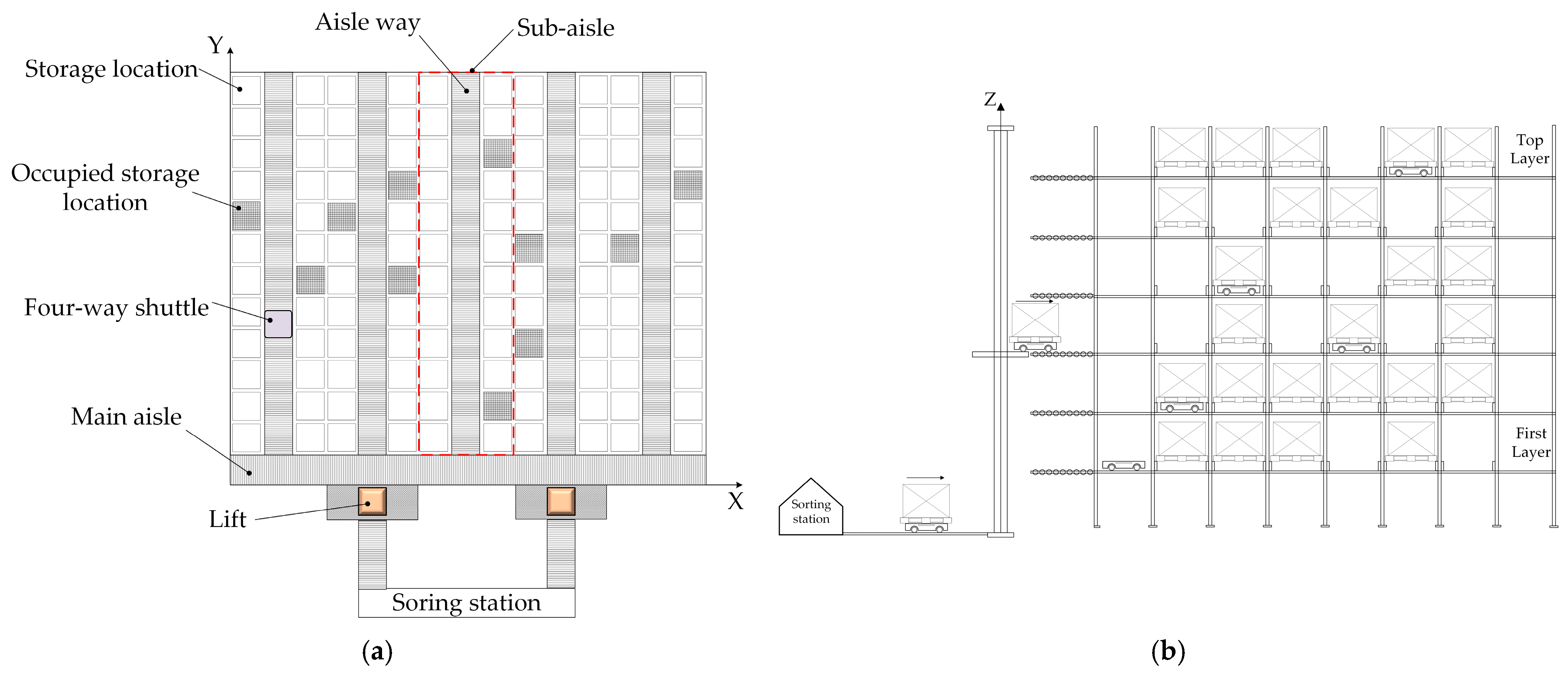
The scenario of Experiment 1 originates from an FWSS/RS of a packaging company, as depicted in Figure 1. Combined with the symbols defined to describe the FWSS/RS task allocation problem, the information related to material handling resources and the warehouse environment is presented in

Table 4. Information related to transport resources and the warehouse environment.

Parameter	Value	Unit	Parameter	Value	Unit
H	1	m	WE	1	m
z	7	—	ashuttle	2	m/s2
R	15	—	$V_{\mathrm{shuttle}}^{\max }$	2	m/s
C	13	—	alift	1	m/s2
WA	1	m	$V_{\mathrm{lift}}^{\max }$	2	m/s
WB	1	m	$F_{11}^{*}$	2	—
WC	1	m	$F_{12}^{*}$	4	—

. Experiment 1 involves three four-way shuttles, two lifts, and 40 material handling tasks. Specifically, the number of inbound tasks is equal to that of the outbound tasks. To facilitate distinguishing tasks with different attributes, the indices of the inbound tasks are defined as 1–20, while those of the outbound tasks are defined as 21–40. The destinations of the inbound tasks and the starting locations of the outbound tasks are shown in

Table 5. Task information.

Task Index	Destination			Task Index	Starting Location
	Column Index	Row Index	Layer Index		Column Index	Row Index	Layer Index
1	7	5	6	21	4	3	4
2	6	5	6	22	7	9	1
3	3	11	1	23	3	2	2
4	4	12	2	24	3	8	5
5	5	6	3	25	2	8	4
6	7	7	4	26	5	1	6
7	6	11	4	27	5	3	6
8	5	11	5	28	8	12	1
9	7	11	2	29	7	11	6
10	9	6	6	30	2	1	6
11	3	6	5	31	9	2	6
12	2	11	7	32	4	2	2
13	8	8	3	33	9	11	3
14	5	7	1	34	4	8	6
15	7	9	3	35	9	3	2
16	4	11	5	36	3	3	4
17	2	6	3	37	3	4	5
18	9	11	4	38	7	3	3
19	4	12	5	39	3	8	4
20	2	5	3	40	3	4	6

. Moreover, when the tasks were assigned simultaneously, all shuttles were located at the sorting station. Correspondingly, based on material handling resources and task information, the settings of estimation and target networks are shown in

Table 6. Estimation and target network structure parameters.

Network Layer	Number of Nodes	Activation Function
Input layer	81	/
Hidden layer 1	128	ReLU
RNN layer	128	ReLU
Hidden layer 2	64	ReLU
Output layer	80	/

.

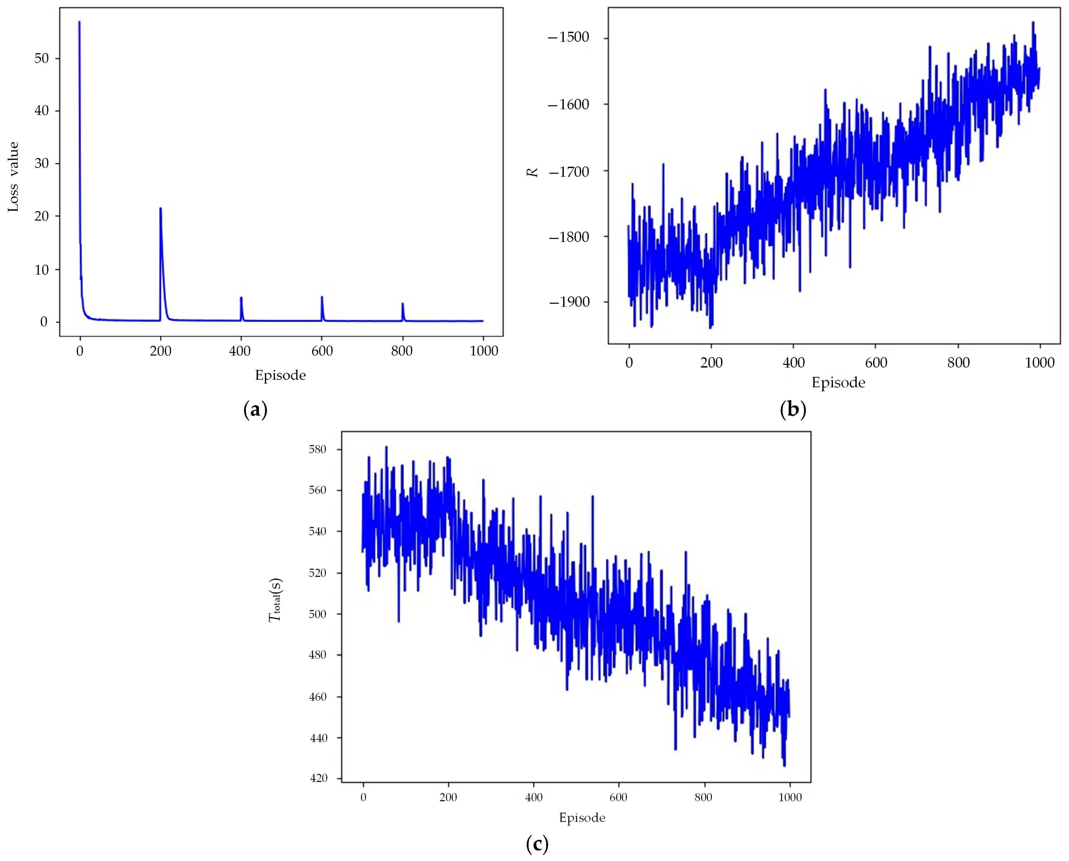
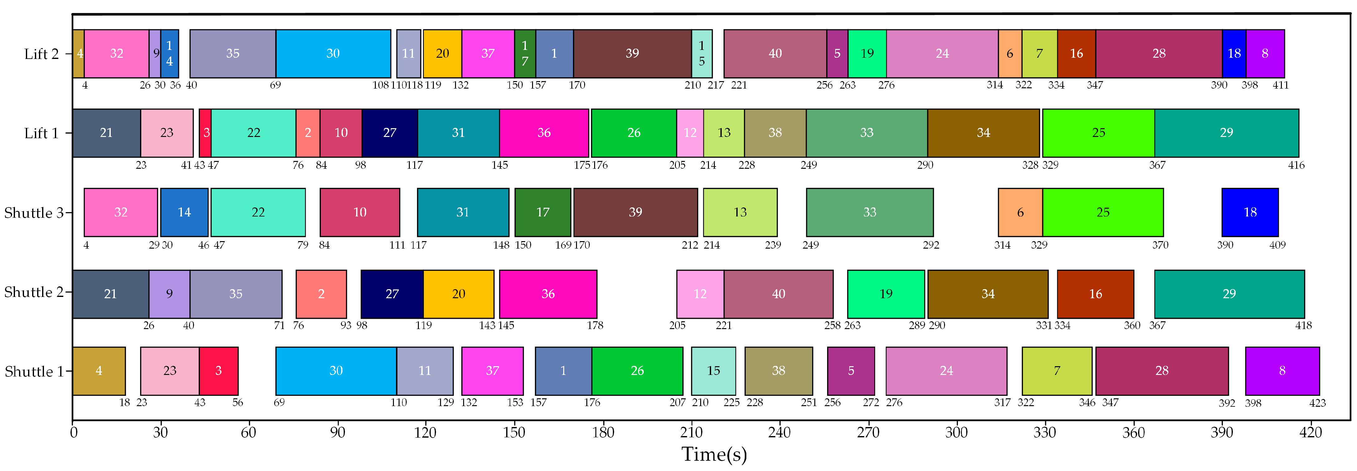
Figure 8 shows the changes in the loss function, reward, and optimization objective during the IDQN training process. It can be observed that as the training proceeds, the IDQN algorithm tends to converge. Correspondingly, the optimal result of task allocation can be presented in the form of a Gantt chart, as depicted in Figure 9.

Moreover, to verify the effectiveness of the IDQN method utilized in this study, the optimal task allocation results obtained by the IDQN were compared with those obtained by two representative task allocation methods, the auction algorithm and the GA. The auction algorithm, which mimics market auction mechanisms for task allocation, offers notable problem-solving efficiency and scalability. It comprises four key components: participants, auction items, profit functions, and bidding strategies. Based on the classic auction algorithm [36] and the characteristics of the task allocation problem in this study, the auction algorithm that integrates a two-stage auction mechanism was used to allocate tasks listed in Table 5, and its workflow is illustrated in Figure 10. The first round of bidding is to match a suitable shuttle for the task, and the second round of bidding is to determine the best lift that can collaborate with the selected shuttle to perform the task. Correspondingly, Figure 11 presents an optimal task allocation result obtained by running the auction algorithm five times.

In addition, the FWSS/RS task allocation problem was solved by the GA, and the key steps were designed as follows.

(1)

Encoding scheme: According to the nature of the FWSS/RS task allocation problem, the chromosome of an individual representing a feasible problem solution is encoded in a hierarchical manner, and its length is equal to the total number of tasks to be executed. The first layer, named the task layer, records the task information; the second layer, named the shuttle layer, records the shuttle resources applied for executing tasks; the third layer, named the lift layer, records the lifts that cooperate with the shuttles to perform tasks. A single gene on the chromosome can be represented in the form of (i, j, l), which means that for task i, shuttle j is responsible for its horizontal transport, and lift l is responsible for its vertical transport.

(2)

Decoding scheme: Decoding is to obtain the values of the decision variables in the model and calculate the values of the optimization objective, thereby evaluating the fitness of an individual. Here, the fitness function is defined as Formula (13). If all tasks are issued at time t and both the shuttle and lift resources are available at that moment, then the initial values of $T_j^{\mathrm{shuttle}}$ and $T_l^{\mathrm{lift}}$ are both set to t. The following are the specific steps for decoding an individual.

Step 1: Scan the chromosome genes from left to right to extract the shuttle and elevator selected to execute the task related to each gene and determine the tasks and sequence to be executed by each shuttle and each lift. Accordingly, based on the individual encoding scheme, the values of the decision variables X_ij and X_il can be determined.

Step 2: Extract each gene from left to right and determine the starting time of each task ($T_i^{\mathrm{start}}$) associated with each gene. Taking the gene (i, j, l) as an example, the execution of task i requires the invocation of shuttle j and lift l. If the tasks executed by shuttle j and lift l adjacent before task i are task i′ and task i″, respectively, then according to research assumption (8), $T_j^{\mathrm{shuttle}}=T_{i\prime }^{\mathrm{end}}$, and $T_l^{\mathrm{lift}}=T^{i″l}$. Consequently, $T_i^{\mathrm{start}}$ can be determined, and $T_i^{\mathrm{start}}=\max \{T_j^{\mathrm{shuttle}},T_l^{\mathrm{lift}}\}$.

Step 3: Based on the position information of the shuttle and the lift, as well as the starting and destination positions of task i, calculate the completion time of task i ($T_i^{\mathrm{end}}$) using Formulas (10)–(12).

Step 4: After the completion of task i, shuttle j and lift l stay at the target position and the target floor of task i, respectively. Record and update the position information of shuttle j and lift l.

Step 5: Repeat steps (2) to (4) until all genes have been decoded. Then, T_total can be determined based on the decoded $T_i^{\mathrm{end}}$ and Formula (13).

(3)

Population initialization scheme: According to the individual encoding scheme, during the initialization of the population, the individual chromosome is initialized layer by layer. First, the real numbers representing tasks are randomly distributed across the gene loci on the first layer of the individual chromosome. Then, a shuttle and a lift are randomly selected for each task from left to right, and the indices of the selected shuttle and lift are assigned to the corresponding gene loci in the shuttle layer and lift layer, respectively.

(4)

Selection operation: In addition to the roulette wheel selection strategy, the elitist retention strategy is also employed, i.e., the best individual in the current population is preserved for the next generation during the evolution process.

(5)

Crossover operation: The commonly used two-point crossover operator [37] is employed. According to the encoding scheme, illegal offspring will not be generated after crossover, but the values of the decision variables X_ij and X_ij will be changed accordingly.

(6)

Mutation operation: Due to the layered coding of individual chromosomes, three mutation operators are designed: ① randomly select two gene loci and swap the genes on the task layer to alter the task execution order; ② randomly select a gene locus and change the gene on the shuttle layer to alter the shuttle resource for executing the task; and ③ randomly select a gene locus and change the gene on the lift layer to change the lift resource for executing the task. The values of the decision variables X_ij and/or X_ij will be changed according to the selected crossover operator.

As for the basic GA parameters, the crossover probability, the mutation probability, the population size, and the maximum number of iterations were set to 0.8, 0.1, 50, and 500, respectively. After running the GA five times, an optimal task allocation scheme was obtained, as presented in Figure 12.

5.2. Experiment 2

Experiment 1 verified the convergence and effectiveness of the MARL method adopted for solving the FWSS/RS task allocation problem. In Experiment 2, the scenario in Experiment 1 was extended, and the performance of different algorithms in handling tasks of various scales and transport resource configurations was compared. The experimental design parameters were selected as the number of shuttles, lifts, inbound tasks, and outbound tasks, with each parameter set at three levels. Accordingly, an L9(3⁴) orthogonal experiment was performed, and the level values of each factor, sorted in ascending order, corresponded to level indices 1, 2, and 3, respectively. Note that, to evaluate the impact of task categories on algorithm performance and maintain consistency with the parameter level settings of the orthogonal experiment, a set of inbound tasks and a set of outbound tasks were added. Then, indices 21–30 were assigned to the newly added inbound tasks. The indices of the outbound tasks in Table 5 were updated to 31–50, while indices 51–60 were allocated to the newly added outbound tasks. Furthermore, the inbound and outbound tasks were evenly divided into three groups according to the index order, respectively. In the orthogonal experiment, when the number of inbound tasks was 10, only tasks with indices 1–10 were involved. When the inbound tasks increased to 20, tasks with indices 1–20 were involved. Similarly, for the outbound job tasks, a quantity of 10 corresponded to tasks with indices 31–40, and when the quantity was 20, it involved tasks with indices 31–50. The information about the newly added inbound and outbound tasks is shown in

Table 7. Information on the newly added tasks.

Task Index	Destination			Task Index	Starting Location
	Column Index	Row Index	Layer Index		Column Index	Row Index	Layer Index
21	3	10	4	51	4	6	5
22	4	8	3	52	5	4	6
23	8	9	2	53	7	5	3
24	9	3	6	54	6	8	5
25	6	10	5	55	10	4	6
26	6	4	3	56	2	2	4
27	5	1	4	57	4	7	3
28	2	4	6	58	5	6	1
29	3	5	5	59	4	7	2
30	5	6	4	60	6	8	6

. Furthermore, all shuttles were initially located at the sorting station, and the newly added lifts were still located in the same sub-aisles as the original lifts in Experiment 1.

Furthermore, based on the orthogonal experiment designed, the optimal T_total achieved by running different methods with the parameter settings in Experiment 1 five times, and the improvement rate of the IDQN solution compared to two comparison algorithms are presented in

Table 8. Comparison of task allocation results.

Example No.	Parameter				Ttotal/s			Improvement Rate of the IDQN Solution
	Number of Shuttles	Number of Lifts	Number of Inbound Tasks	Number of Outbound Tasks	Auction Algorithm	GA	IDQN	Auction Algorithm	GA
1	3	2	10	10	235	228	211	10.21%	7.45%
2	3	4	20	20	374	363	346	7.48%	4.68%
3	3	6	30	30	556	545	519	6.65%	4.77%
4	4	2	20	30	610	585	535	12.29%	8.54%
5	4	4	30	10	317	310	291	8.2%	6.12%
6	4	6	10	20	230	226	210	8.69%	7.07%
7	5	2	30	20	587	569	529	9.88%	7.02%
8	5	4	10	30	291	280	258	11.3%	7.85%
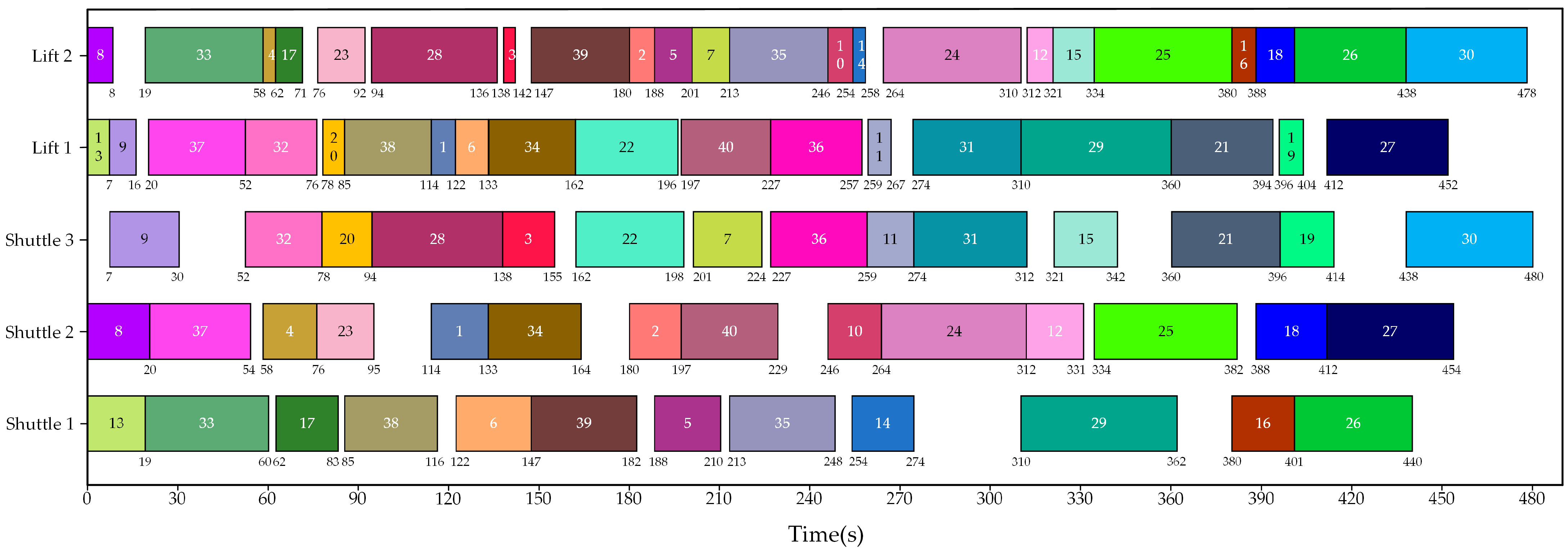
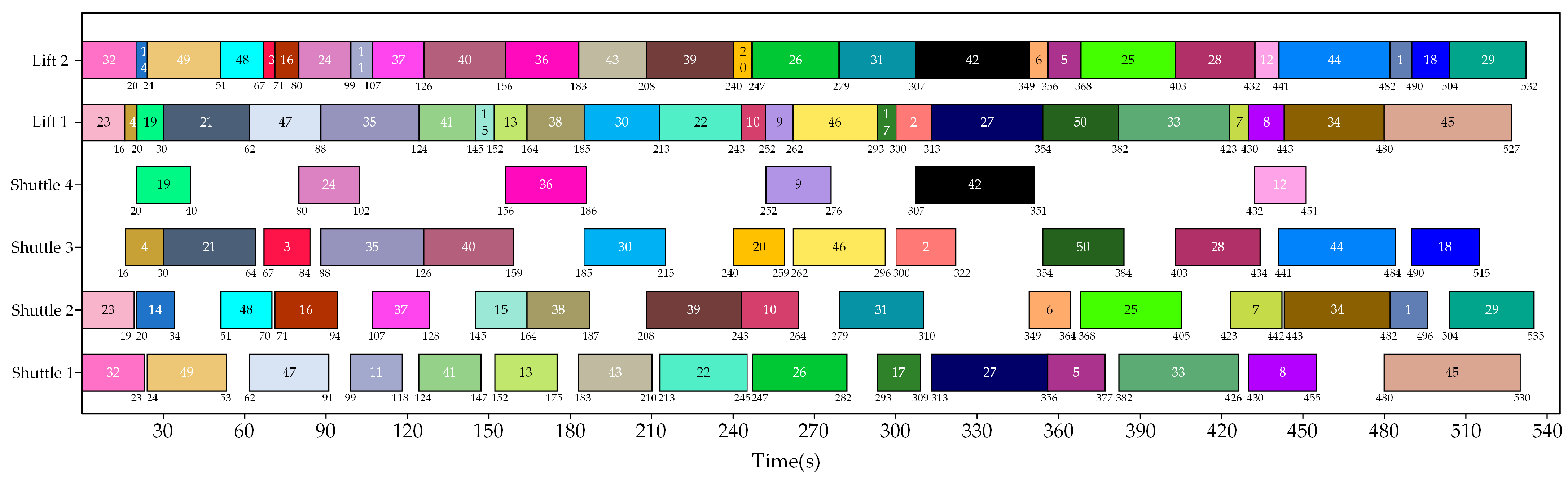
9	5	6	20	10	194	185	169	12.88%	8.64%

. Specifically, the minimum T_total was obtained in Example 4, while the maximum T_total was obtained in Example 9. Correspondingly, the optimal task allocation schemes acquired by the IDQN in such two examples are presented in Figure 13 and Figure 14, respectively.

In addition, two comparative experiments were conducted under the transport resource configuration of three shuttles and two lifts, and they can be referred to as Examples 10 and 11 based on the orthogonal experimental scenarios in Table 8. Example 10 involves 10 inbound tasks and 30 outbound tasks, while Example 11 involves 30 inbound tasks and 10 outbound tasks. Accordingly, the optimal T_total acquired by the IDQN corresponding to such two examples was 485 s and 461 s, respectively.

5.3. Discussion

In Experiment 1, the convergence analysis of the loss function reveals that it rapidly decreases in the early stages of training and stabilizes within a relatively short number of training steps, as shown in Figure 8a. This can be attributed to the following key factors:

(1)

Efficient Q-value approximation: The IDQN adopts the PER mechanism, which reduces sample correlation and improves training stability. A target network is also introduced to mitigate Q-estimation fluctuations, enabling faster convergence to a reasonable Q-estimation and accelerating the decline of the loss function.

(2)

Gradient optimization characteristics: In DRL, the loss function minimizes TD_error between predicted and target Q-values. In early training, the large TD_error leads to bigger gradients, enabling quick adjustment of neural network parameters and a rapid decline in the loss function. As training proceeds and the error gradually shrinks, gradient updates will slow down, stabilizing the loss function.

(3)

Value function learning and policy optimization: Unlike policy gradient methods, Q-learning-based approaches first train the value function to converge to accurate Q-estimations, then improve the policy via a greedy strategy. Although the loss function converges early, the agent’s policy continues to optimize, causing the reward function to converge more slowly.

As shown in Figure 8, after starting the training, the loss function, reward function, and the T_total all improve with the increase in the number of training episodes. It can be observed that the algorithm’s performance metrics stabilize within a certain range after 900 episodes. This indicates that the IDQN algorithm is effective for solving the proposed model. Note that the loss function oscillates every 200 steps. The reason for this phenomenon is that under the IDQN algorithm framework, the estimation network needs to assign weights to the target network after a certain number of training steps. However, the amplitude of these oscillations will decrease with the increase in training steps.

According to Figure 9, Figure 11 and Figure 12, the IDQN outperforms the auction algorithm and the GA in Experiment 1. Further analysis of the optimal task allocation scheme reveals that if a shuttle, after completing an inbound task, is subsequently assigned an outbound task, it is beneficial to shorten the pickup stage time of the outbound task, thereby reducing the total task completion time (T_total). Meanwhile, due to the inevitable utilization of lifts in task execution, the utilization rate of lifts reflects the superiority or inferiority of the task allocation schemes to some extent.

Table 9. Comparison of the optimal task allocation schemes in terms of transport equipment utilization and T_total.

Indicator		IDQN	Auction Algorithm	GA
Shuttle utilization rate	Shuttle 1	87.71%	82.05%	83.95%
	Shuttle 2	86.84%	85.68%	85.68%
	Shuttle 3	82.72%	81.82%	85.29%
Average shuttle utilization rate		85.76%	83.18%	84.97%
Lift utilization rate	Lift 1	99.04%	94.25%	98.42%
	Lift 2	97.32%	93.10%	94.76%
Average lift utilization rate		98.18%	93.68%	96.59%
Total equipment utilization rate		91.97%	88.43%	90.78%
Total task completion time (Ttotal)		423 s	480 s	461 s

presents the comparison of the optimal task allocation schemes obtained by three algorithms in T_total and indicators related to transport equipment utilization.

Regardless of which method is adopted for task allocation, lifts are generally much busier than shuttles. From the perspective of individual equipment utilization, when employing the IDQN for task allocation, lift 1 achieves the highest utilization rate at 99.04%. Meanwhile, although the utilization rate of shuttle 3 is not the highest, the total equipment utilization rate is the highest due to the efficient utilization of the vast majority of transport resources. Moreover, the IDQN outperforms the other two algorithms in terms of T_total, which indicates that the strategies learned by the IDQN not only focus on maximizing the utilization of each piece of equipment but also on the coordination and scheduling of transport resources at the system level.

In Experiment 2, an orthogonal experiment was designed and conducted to verify whether the IDQN still had advantages in different scenarios and investigate the impact of transport resource configuration and task attributes on task allocation. It can be observed from Table 8 that the IDQN achieves superior results compared to the other two algorithms in all nine scenarios of the orthogonal experiment. Furthermore, combined with the optimal T_total obtained by the IDQN, a range analysis was conducted to identify the degree of influence of various factors on the results. 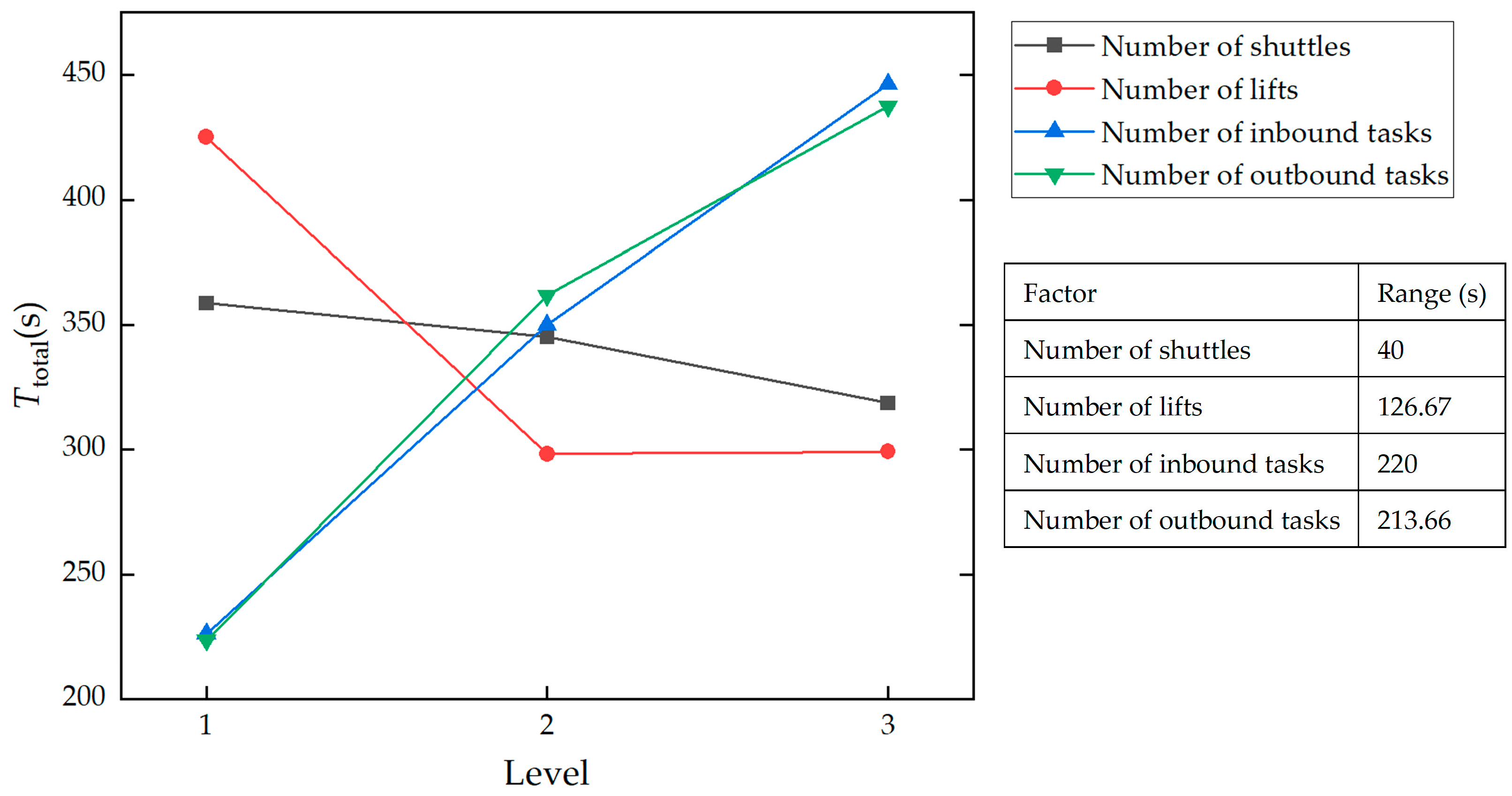Figure 15 depicts the trend of factor levels in the orthogonal experiment.

From Figure 15, the order of influence of various factors on the results can be derived, i.e., Number of inbound tasks > Number of outbound tasks > Number of lifts > Number of shuttles. Specifically, inbound and outbound task volumes are the core influencing factors. An increase in task volume will exacerbate the difficulty of equipment collaborative scheduling and prolong the completion time. Among transport resources, the number of lifts is more critical than that of shuttles, which is consistent with the characteristic of lifts as vertical material handling bottlenecks in warehousing systems. Both an excess and a shortage of lifts can easily induce waiting delays. The range of the number of shuttles is the smallest, and the average T_total decreases with more shuttles, but the reduction is limited. This indicates that adding shuttles within the experimental scope can slightly shorten T_total, but the number of shuttles is not a key control point of the warehouse system. In practical applications, shuttle deployment should be based on a cost-benefit analysis.

Furthermore, based on the orthogonal experiment data in Table 8, an analysis of variance was conducted to identify whether different factors have a significant impact on the T_total. However, in the orthogonal experiment, the initial degree of freedom of error was 0, preventing the F-value calculation. Therefore, according to the results of the range analysis and the sum of squares of each factor, the insignificant factor, i.e., the number of shuttles, was merged to release the degrees of freedom. The variance analysis results are shown in

Table 10. Analysis of variance results.

Source	Sum of Squares	Degrees of Freedom	Mean Square	F-Value	p-Value
Number of lifts	31,840.17	2	15,920.08	12.78	0.074
Number of inbound tasks	72,968.16	2	36,484.08	29.29	0.032
Number of outbound tasks	70,426.35	2	35,213.18	28.27	0.034
Error	2490.95	2	1245.48	-	-
Total	177,725.63	8	-	-	-

. If the significance level is set at 0.05, the null hypothesis can be rejected for factors related to inbound and outbound tasks. Their p-values are both less than 0.05, thus indicating that both factors exert a statistically significant effect on the outcome. Meanwhile, for the factor related to lifts, the null hypothesis cannot be rejected as the corresponding p-value is greater than 0.05. However, it is less than 0.1, which suggests that this factor is marginally significant at the significance level 0.1.

In addition, combining the experimental data from Experiment 1 and two comparative experiments in Experiment 2, it can be observed that the ratio of inbound tasks to outbound tasks also affects the task allocation results when transport resources and the total amount of tasks are determined. In the experimental study, all shuttles were assumed to be initially at the sorting station. When a batch of tasks with more outbound ones was issued, the pickup phase time related to outbound tasks was relatively long, resulting in a longer total task completion time. However, when the proportion of inbound and outbound tasks was balanced, after a shuttle completed an inbound task, it could immediately perform an outbound task since it had already entered the rack layer. This saved pickup time compared with the shuttle entering the rack layer from the sorting station. Similarly, when a shuttle was immediately assigned an inbound task after completing an outbound task, the execution of the inbound task directly entered the delivery stage, thus improving the efficiency of task execution. In practical applications, since hardware resources are not easily changed, it is essential to consider both task issuance volume and the proportion of different task types to fully and efficiently utilize transport equipment.

6. Conclusions

This study focuses on the task allocation problem in an FWSS/RS under the composite operation mode, and the main contributions are summarized as follows: (1) A comprehensive mathematical model is established to capture the dynamic characteristic of shuttle–lift cooperation in FWSS/RSs and optimize the overall task completion time. (2) A decentralized learning framework based on IDQN is introduced to address the task allocation problem, enabling scalable and autonomous task allocation decisions across multiple agents. (3) The advantages of the IDQN-based task allocation method over conventional ones (the auction algorithm and the GA) are demonstrated through the experimental study. (4) The number and type of tasks significantly affect system performance, highlighting the importance of a balanced task structure and sufficient vertical transport capacity in FWSS/RS design.

Despite the promising performance of the proposed IDQN-based task allocation approach, several limitations should be acknowledged to contextualize its scope and applicability. The current model assumes a static task set and does not consider dynamically arriving tasks, fluctuating order priorities, or unpredictable equipment failures, which are common in real-world warehousing operations. Moreover, shuttle path conflicts, energy consumption, and potential lift malfunctions have been simplified or omitted in the simulation environment, potentially affecting the model’s applicability to actual deployments. In addition, although each shuttle operates as an independent agent within a decentralized framework, no explicit inter-agent communication or coordination mechanism has been implemented, which may limit global optimization in highly complex environments.

Consequently, future research will focus on the following: (1) enhancing the algorithm’s generalization to handle uncertainties like dynamic task arrivals, changing order priorities, and equipment failures; (2) improving deep neural network models and the MARL architecture to improve the efficiency of decision-making and collaboration among multiple agents; (3) exploring the feasibility of deploying the method in real engineering application scenarios; (4) exploring potential trade-offs between computational complexity and scheduling performance and developing multi-objective optimization strategies that incorporate energy efficiency, equipment reliability, and overall system robustness under dynamic operational conditions.

References

1. Wang, X.; Dong, F. The dynamic relationships among growth in the logistics industry, energy consumption, and carbon emission: Recent evidence from China. J. Pet. Explor. Prod. Technol. 2023, 13, 487–502. [Google Scholar] [CrossRef]
2. Liu, X.; Liu, X.; Song, Y.; Hu, Y.; Zhou, L.; Xu, X. An Accurate and Rapid Docking Algorithm for Four-Way Shuttle in High-Density 3D Warehousing Environment. Machines 2024, 12, 435. [Google Scholar] [CrossRef]
3. Boysen, N.; Stephan, K. A survey on single crane scheduling in automated storage/retrieval systems. Eur. J. Oper. Res. 2016, 254, 691–704. [Google Scholar] [CrossRef]
4. Li, Y.; Li, Z. Shuttle-based storage and retrieval system: A literature review. Sustainability 2022, 14, 14347. [Google Scholar] [CrossRef]
5. Cinar, Z.; Zeeshan, Q. Design and optimization of automated storage and retrieval systems: A review. In Industrial Engineering in the Internet-of-Things World, Proceedings of the Global Joint Conference on Industrial Engineering and Its Application Areas, Antalya, Türkiye, 14–15 August 2020; Springer: Cham, Switzerland, 2022; pp. 177–190. [Google Scholar] [CrossRef]
6. Yang, X.; Rahmani, N. Task scheduling mechanisms in fog computing: Review, trends, and perspectives. Kybernetes 2021, 50, 22–38. [Google Scholar] [CrossRef]
7. Waubert de Puiseau, C.; Nanfack, D.T.; Tercan, H.; Löbbert-Plattfaut, J.; Meisen, T. Dynamic storage location assignment in warehouses using deep reinforcement learning. Technologies 2022, 10, 129. [Google Scholar] [CrossRef]
8. Kuhn, H.W. The Hungarian method for the assignment problem. Nav. Res. Logist. 2010, 52, 7–21. [Google Scholar] [CrossRef]
9. Martin, J.G.; Frejo, J.R.D.; Garcia, R.A.; Camacho, E.F. Multi-robot task allocation problem with multiple nonlinear criteria using branch and bound and genetic algorithms. Intell. Serv. Robot. 2021, 14, 707–727. [Google Scholar] [CrossRef]
10. Ma, T.; Lu, P.; Deng, F.; Geng, K. Air-ground collaborative multi-target detection task assignment and path planning optimization. Drones 2024, 8, 110. [Google Scholar] [CrossRef]
11. Qiu, Z.; Long, J.; Yu, Y.; Chen, S. Integrated task assignment and path planning for multi-type robots in an intelligent warehouse system. Transp. Res. Part E Logist. Transp. Rev. 2025, 194, 103883. [Google Scholar] [CrossRef]
12. Baroudi, U.; Alshaboti, M.; Koubaa, A.; Trigui, S. Dynamic multi-objective auction-based (DYMO-Auction) task allocation. Appl. Sci. 2020, 10, 3264. [Google Scholar] [CrossRef]
13. Li, J.; Liu, K.; Wang, H. Task assignment optimization of multi-logistics robot based on improved auction algorithm. In Proceedings of the 9th International Conference on Logistics, Informatics and Service Sciences; Springer: Singapore, 2020; pp. 41–54. [Google Scholar] [CrossRef]
14. Chen, R.; Yang, J.; Yu, Y.; Guo, X. Retrieval request scheduling in a shuttle-based storage and retrieval system with two lifts. Transp. Res. Part E Logist. Transp. Rev. 2023, 174, 103117. [Google Scholar] [CrossRef]
15. D’Antonio, G.; Chiabert, P. Analytical models for cycle time and throughput evaluation of multi-shuttle deep-lane AVS/RS. Int. J. Adv. Manuf. Technol. 2019, 104, 1919–1936. [Google Scholar] [CrossRef]
16. Zhou, J.; Zhao, X.; Zhang, X.; Zhao, D.; Li, H. Task allocation for multi-agent systems based on distributed many-objective evolutionary algorithm and greedy algorithm. IEEE Access 2020, 8, 19306–19318. [Google Scholar] [CrossRef]
17. Nedjah, N.; Mendonça, R.M.D.; Mourelle, L.D.M. PSO-based distributed algorithm for dynamic task allocation in a robotic swarm. Procedia Comput. Sci. 2015, 51, 326–335. [Google Scholar] [CrossRef]
18. Asma, A.; Sadok, B. PSO-based dynamic distributed algorithm for automatic task clustering in a robotic swarm. Procedia Comput. Sci. 2019, 159, 1103–1112. [Google Scholar] [CrossRef]
19. Gao, J.; Li, Y.; Xu, Y.; Lv, S. A two-objective ILP model of OP-MATSP for the multi-robot task assignment in an intelligent warehouse. Appl. Sci. 2022, 12, 4843. [Google Scholar] [CrossRef]
20. Wei, C.; Ji, Z.; Cai, B. Particle swarm optimization for cooperative multi-robot task allocation: A multi-objective approach. IEEE Robot. Autom. Lett. 2020, 5, 2530–2537. [Google Scholar] [CrossRef]
21. Li, J.; Yang, F. Task assignment strategy for multi-robot based on improved grey wolf optimizer. J. Ambient. Intell. Humaniz. Comput. 2020, 11, 6319–6335. [Google Scholar] [CrossRef]
22. Guo, H.; Miao, Z.; Pan, Q. An effective collaboration evolutionary algorithm for multi-robot task allocation and scheduling in a smart farm. Knowl.-Based Syst. 2024, 289, 111474. [Google Scholar] [CrossRef]
23. Ekren, B.Y.; Arslan, B. A reinforcement learning approach for transaction scheduling in a shuttle-based storage and retrieval system. Int. Trans. Oper. Res. 2024, 31, 274–295. [Google Scholar] [CrossRef]
24. Gong, A.; Yang, K.; Lyu, J.; Li, X. A two-stage reinforcement learning-based approach for multi-entity task allocation. Eng. Appl. Artif. Intell. 2024, 136, 108906. [Google Scholar] [CrossRef]
25. Wu, S.; Chiu, W.; Wu, C. Deep Reinforcement learning for task assignment and shelf reallocation in smart warehouses. IEEE Access 2024, 12, 58915–58926. [Google Scholar] [CrossRef]
26. Li, Z.; Shi, N.; Zhao, L.; Zhang, M. Deep reinforcement learning path planning and task allocation for multi-robot collaboration. Alex. Eng. J. 2024, 109, 408–423. [Google Scholar] [CrossRef]
27. Dai, Y.; Kim, D.; Lee, K. Development of a fleet management system for multiple robots’ task allocation using deep reinforcement learning. Processes 2024, 12, 2921. [Google Scholar] [CrossRef]
28. Agrawal, A.; Hariharan, S.; Bedi, A.S.; Manocha, D. DC-MRTA: Decentralized multi-robot task allocation and navigation in complex environments. In Proceedings of the 2022 IEEE/RSJ International Conference on Intelligent Robots and Systems (IROS), Kyoto, Japan, 23–27 October 2022; pp. 11711–11718. [Google Scholar]
29. Hersi, A.H.; Udayan, J.D. Efficient and robust multirobot navigation and task allocation using soft actor critic. Procedia Comput. Sci. 2024, 235, 484–495. [Google Scholar] [CrossRef]
30. Zhu, P.; Dai, W.; Yao, W.; Ma, J.; Zeng, Z.; Lu, H. Multi-robot flocking control based on deep reinforcement learning. IEEE Access 2020, 8, 150397–150406. [Google Scholar] [CrossRef]
31. Elfakharany, A.; Ismail, Z.H. End-to-end deep reinforcement learning for decentralized task allocation and navigation for a multi-robot system. Appl. Sci. 2021, 11, 2895. [Google Scholar] [CrossRef]
32. Zhao, G.; Wang, Y.; Mu, T.; Meng, Z.; Wang, Z. Reinforcement-learning-assisted multi-UAV task allocation and path planning for IIoT. IEEE Internet Things J. 2024, 11, 26766–26777. [Google Scholar] [CrossRef]
33. Tampuu, A.; Matiisen, T.; Kodelja, D.; Kuzovkin, I.; Korjus, K.; Aru, J.; Aru, J.; Vicente, R. Multiagent cooperation and competition with deep reinforcement learning. PLoS ONE 2017, 12, e0172395. [Google Scholar] [CrossRef] [PubMed]
34. Wang, J.; Li, Y.; Zhang, Z.; Wu, Z.; Wu, L.; Jia, S.; Peng, T. Dynamic integrated scheduling of production equipment and automated guided vehicles in a flexible job shop based on deep reinforcement learning. Processes 2024, 12, 2423. [Google Scholar] [CrossRef]
35. Jiang, L.; Huang, H.; Ding, Z. Path planning for intelligent robots based on deep Q-learning with experience replay and heuristic knowledge. IEEE-CAA J. Autom. Sin. 2020, 7, 1179–1189. [Google Scholar] [CrossRef]
36. Eijyne, T.; Rishwaraj, G.; Ponnambalam, S.G. Development of a task-oriented, auction-based task allocation framework for a heterogeneous multirobot system. Sadhana-Acad. Proc. Eng. Sci. 2020, 45, 115. [Google Scholar] [CrossRef]
37. Watanabe, M.; Ida, K.; Gen, M. A genetic algorithm with modified crossover operator and search area adaptation for the job-shop scheduling problem. Comput. Ind. Eng. 2005, 48, 743–752. [Google Scholar] [CrossRef]
Figure 1. Layout of the FWSS/RS: (a) top view; (b) side view.
Sustainability 17 06772 g001
Figure 2. Workflow of a shuttle executing a task.
Sustainability 17 06772 g002
Figure 3. Motion mode of the four-way shuttle: (a) uniform acceleration–uniform deceleration; (b) uniform acceleration–uniform motion–uniform deceleration.
Sustainability 17 06772 g003
Figure 4. Example of transport path in Situation 2.
Sustainability 17 06772 g004
Figure 5. Example of transport path in Situation 3a.
Sustainability 17 06772 g005
Figure 6. Schematic diagram of neural network structure.
Sustainability 17 06772 g006
Figure 7. Flowchart of the IDQN algorithm.
Sustainability 17 06772 g007
Figure 8. Change curves of algorithm performance indicators: (a) loss curve; (b) reward curve; (c) curve of the completion time of all tasks.
Sustainability 17 06772 g008
Figure 9. An optimal task allocation scheme obtained by the IDQN.
Sustainability 17 06772 g009
Figure 10. Flowchart of the auction algorithm.
Sustainability 17 06772 g010
Figure 11. An optimal task allocation scheme obtained by the auction algorithm.
Sustainability 17 06772 g011
Figure 12. An optimal task allocation scheme obtained by the GA.
Sustainability 17 06772 g012
Figure 13. An optimal task allocation scheme acquired by the IDQN for Example 4.
Sustainability 17 06772 g013
Figure 14. An optimal task allocation scheme acquired by the IDQN for Example 9.
Sustainability 17 06772 g014
Figure 15. Trend of factor levels.
Sustainability 17 06772 g015