Hybrid Forecasting Framework for Emergency Material Demand in Post-Earthquake Scenarios Integrating the Grey Model and Bayesian Dynamic Linear Models

Abstract

Earthquakes are sudden and highly destructive events that severely disrupt infrastructure and logistics systems, making accurate and timely emergency material demand forecasting a critical challenge in disaster response. However, the scarcity of reliable data during the early stages of an earthquake limits the effectiveness of traditional forecasting methods. To address this issue, this study proposes a hybrid forecasting framework that integrates the Grey Model (GM(1,1)) with Bayesian Dynamic Linear Models (BDLMs), aiming to improve both the accuracy and adaptability of demand predictions. The approach operates in two phases: first, GM(1,1) generates preliminary forecasts using limited initial observations; second, BDLMs dynamically update these forecasts in real time as new data become available. The model is validated through a case study of the 2010 M7.1 Yushu earthquake in Qinghai Province, China. The results indicate that the hybrid method produces reliable forecasts even at the earliest stages of the disaster, with increasing accuracy as more observational data are incorporated. Our case study demonstrates that the integrated GM(1,1)-BDLM framework substantially reduces prediction errors compared to standalone GM(1,1). Using the first five days’ data to forecast fatalities and emergency material demand for days 6–10, the hybrid model achieves a 4.01% error rate—a 19.62 percentage point improvement over GM(1,1)’s 23.63% error rate. This adaptive forecasting mechanism offers robust support for evidence-based decision-making in emergency material allocation, enhancing the efficiency and responsiveness of post-disaster relief operations.

1. Introduction

China is located at the intersection of the Pacific Ring of Fire and the Eurasian seismic belt, where the ongoing tectonic compression between the Indian and Eurasian plates leads to frequent and intense seismic activity [1]. Since the beginning of the 21st century, numerous provinces and cities across the country have been struck by major earthquakes, resulting in significant human casualties and substantial impacts on economic development and public well-being. Earthquakes are characterized by their sudden onset and unpredictability, making it essential to establish an efficient emergency logistics system after a major seismic event to ensure the timely delivery of critical relief supplies such as food, medicine, and tents to affected areas.

However, the demand for emergency supplies in earthquake disasters is highly uncertain [2], and its dynamic evolution is influenced by a combination of factors, including disaster severity, population affected, and the extent of infrastructure damage. Traditional methods for forecasting emergency material demand—such as expert-based qualitative analysis and statistical regression models [3]—often struggle to address the issue of incomplete or imperfect information in disaster environments. Therefore, improving the accuracy and adaptability of demand forecasting under conditions of limited and uncertain data has become a critical scientific challenge in the field of disaster emergency management [4].

In response to the challenge of forecasting emergency logistics demand in earthquake disasters, existing research has primarily focused on four methodological directions: optimization models, deep learning and big data algorithms, machine learning techniques, and grey prediction methods [5]. Optimization models are mainly used to improve post-disaster resource allocation and distribution strategies [6], such as the Voronoi diagram-based location model for emergency logistics centres, and facility location/allocation optimization models [7]. These models demonstrate notable advantages in optimizing supply transportation routes [8] and resource distribution efficiency [9]. However, their predictive accuracy heavily relies on prior data availability, and they often lack adaptability to dynamically changing demand patterns.

With the rise in big data and deep learning technologies, increasing attention has been devoted to applying these advanced techniques to the dynamic forecasting of emergency material demand. Xue et al. [10] proposed a cluster-based supply chain forecasting approach for emergency supplies by integrating a fuzzy C-means clustering algorithm with a data stream processing framework based on the Long Short-Term Memory (LSTM) network. Similarly, models combining Convolutional Neural Networks (CNNs) with transfer learning have also been applied to forecasting the demand for emergency medical supplies. Chen et al. [11] employed an Improved Ant Colony Optimization–Back Propagation (IACO-BP) algorithm to predict emergency material demand under flood scenarios. The results indicate that this hybrid model can significantly enhance forecasting accuracy.

In recent years, machine learning methods have been increasingly applied to forecasting emergency logistics demand. For instance, He and Zhu [12] employed a Genetic Algorithm-optimized Support Vector Machine (SVM) model to enhance the accuracy of emergency supply forecasting under earthquake scenarios. In addition, some researchers have proposed models that integrate regression analysis with inventory management, which have demonstrated promising predictive performance [13]. Fang et al. [14] applied a Back Propagation (BP) neural network model to estimate the number of affected people and the required amount of medical emergency supplies during the Wenchuan earthquake and further developed a GIS-based emergency medical response system for earthquakes. These studies highlight the advantages of machine learning methods in modelling complex nonlinear relationships in disaster demand forecasting.

However, these methods typically require a large amount of historical data for training, which is often scarce in the case of rare events such as earthquakes, thereby limiting the generalization capability of the models [15]. To address such challenges, Chinese scholar Deng [16] proposed the Grey System Theory in the 1980s, which was specifically designed to handle systems characterized by incomplete information and high uncertainty. In his foundational work, Deng summarized key methodologies of grey systems, including accumulated generating operations [17], differential equation modelling, grey prediction techniques, and grey mathematical programming, laying the theoretical groundwork for the subsequent development of grey forecasting approaches.

Furthermore, Deng and Zhou [18] conducted in-depth research on the stability of grey systems and proposed stability criteria based on non-negative irreducible matrices, providing theoretical support for the application of grey prediction models in dynamic systems.

The grey prediction method has gained widespread attention in the field of disaster forecasting due to its strong applicability in scenarios characterized by limited data and incomplete information. For example, Jiang, A., et al. [19] investigated the impact of linear transformations on the accuracy of grey models and found that appropriate parameter adjustments can significantly improve predictive performance. Ma, X., et al. [20] proposed a Grey Model (GM(1,1)) based on composite Simpson’s rule and standard deviation adjustment, further enhancing forecasting accuracy through parameter optimization. Additionally, other improved approaches, such as the grey Euler optimization model, have also shown promising results in improving the accuracy of grey predictions [21]. However, the traditional GM(1,1) still faces challenges such as delayed information updating and limited environmental adaptability during the forecasting process. Therefore, how to further optimize grey prediction methods to better accommodate the dynamic changes in disaster environments remains an important topic requiring in-depth investigation.

Although the aforementioned methods have achieved certain successes in different aspects, they still exhibit significant limitations. Single forecasting models often lack sufficient adaptability to dynamically changing post-disaster demand patterns [22] and fail to adequately account for the grey uncertainty inherent in earthquake emergency logistics [23]. To address these issues, this study proposes a hybrid forecasting approach for emergency logistics demand in earthquake disasters that integrates the GM(1,1) with Bayesian Dynamic Linear Models (BDLMs), aiming to enhance both predictive accuracy and dynamic adaptability. The application of Bayesian methods in forecasting has been extensively discussed in the literature, highlighting their capacity for handling uncertainty and dynamically updating predictions in response to new information. West and Harrison [24] emphasize the importance of incorporating prior information and adapting models as more data becomes available, which aligns with the objectives of this research. By combining Grey System Theory with dynamic Bayesian modelling, the proposed method constructs a forecasting framework with a mechanism for real-time parameter updating, thereby providing a more scientifically grounded basis for decision-making in emergency supply dispatching.

Specifically, the GM(1,1) demonstrates strong short-term forecasting performance under small-sample conditions, while the BDLM enables continuous information updating and assimilation of newly available data, effectively capturing the evolving nature of post-disaster demand. The complementary strengths of these two models significantly enhance the overall adaptability of the forecasting system to the dynamic evolution of disaster situations. Particularly in response to the continuously updating nature of post-disaster information, this study designs a real-time forecasting adjustment mechanism based on BDLMs, allowing the prediction results to be dynamically optimized as the disaster unfolds. This research not only overcomes the limitations of single-model forecasting but, more importantly, establishes a prediction framework with dynamic responsiveness, contributing both theoretical innovation and practical guidance to the field of disaster emergency management.

The integrated GM(1,1)-BDLM framework enhances emergency logistics forecasting through improved prediction accuracy and dynamic adaptability, enabling more precise data-driven resource allocation. This advancement directly supports the following: (1) SDG 11.5’s target of reducing disaster economic losses, (2) China’s 14th Five-Year National Comprehensive Disaster Prevention Plan’s requirements for intelligent forecasting systems, and (3) the low-carbon emergency logistics provisions under the State Council’s Green Logistics Guidelines. By bridging predictive modelling innovation with sustainable disaster governance, the research contributes to both operational efficiency and policy implementation.

2. Methods

2.1. Conceptual Framework and Modelling Strategy

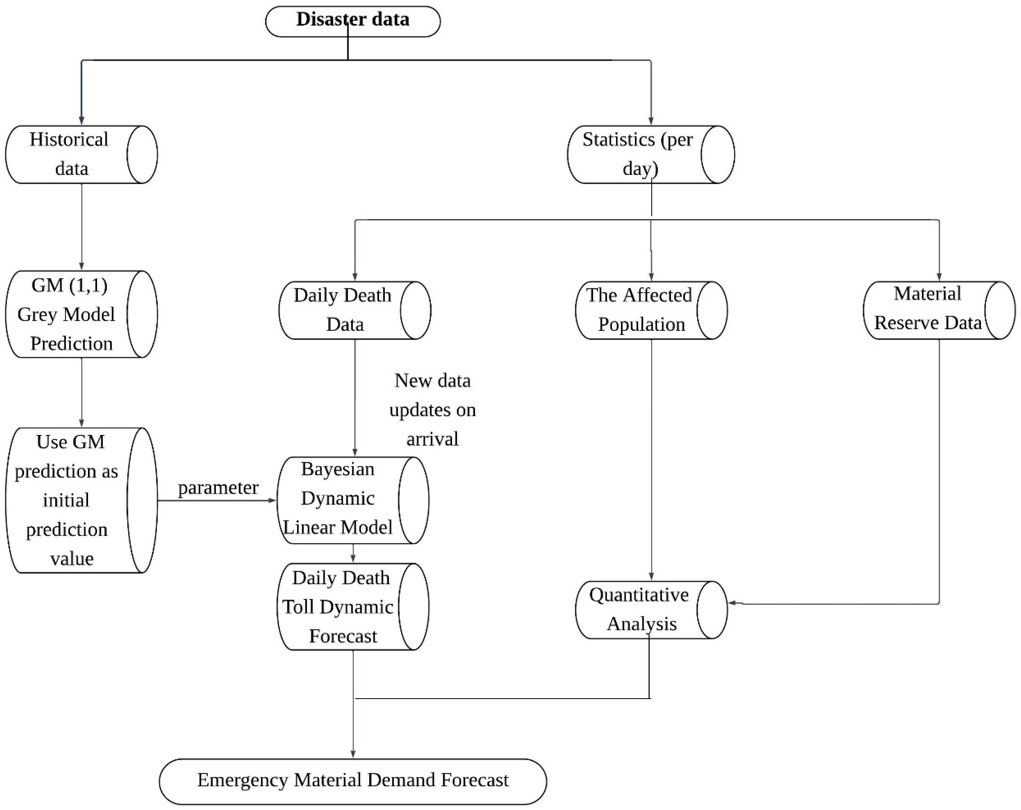
This study constructs a forecasting workflow for emergency material demand that integrates historical data analysis, dynamic modelling, and quantitative evaluation. First, multi-source information is extracted from disaster-related data, including historical mortality records, daily statistical reports, and emergency supply inventory levels.

For the historical mortality data, the GM(1,1) grey prediction model is employed to generate an initial trend forecast. The resulting predictions are then used as prior inputs for the BDLMs, which dynamically update and forecast daily mortality figures, thereby enabling real-time monitoring of the evolving disaster situation. Concurrently, quantitative analysis is conducted based on the updated mortality and affected population data, in conjunction with current supply inventory levels, to assess resource matching status and identify potential shortage risks.

Based on this integrated analysis, the system can scientifically forecast future emergency material demand over a short time horizon, providing efficient and accurate decision support for government authorities and emergency management agencies during disaster response. The entire process realizes data-driven dynamic forecasting and optimized resource allocation, offering strong practical applicability and scalability. The overall conceptual framework is illustrated in Figure 1.

2.2. Mortality Forecasting Using Grey Model and BDLMs

2.2.1. GM(1,1) for Mortality Forecast

GM(1,1) is a forecasting method specifically designed for small-sample and uncertain systems. Its core idea lies in transforming a stochastic sequence into a more regular one through data processing, and then constructing a predictive model based on a grey differential equation. This approach overcomes the limitations of traditional regression analysis, which typically requires large sample sizes and assumes specific data distributions. Therefore, GM(1,1) is particularly suitable for demand forecasting in the early stages of an earthquake when data availability is limited.

In this study, the mean GM(1,1) is first applied to forecast the number of fatalities in the disaster-affected areas. The detailed construction process is as follows:

$$\begin{array}{c}{X}^{\left(0\right)}=\left(x^{\left(0\right)}\left(1\right),{ x}^{\left(0\right)}\left(2\right),\cdots ,{ x}^{\left(0\right)}\left(t\right)\right)\end{array}$$

(1)

denote the original sequence of mortality data, where $x^{\left(0\right)}\left(t\right)$ represents the number of fatalities in the earthquake-affected area at time t.

$X^{\left(1\right)}$ denotes the 1-AGO sequence of $X^{\left(0\right)}$:

$$\begin{array}{c}{X}^{\left(1\right)}=\left(x^{\left(1\right)}\left(1\right),{ x}^{\left(1\right)}\left(2\right),\cdots ,{ x}^{\left(1\right)}\left(t\right)\right)\end{array}$$

(2)

where

$$\begin{array}{c}{x}^{\left(1\right)}\left(k\right)={\sum }_{i=1}^k{x}^{\left(0\right)}\left(i\right), k=1, 2,\dots , t\end{array}$$

(3)

$Z^{\left(1\right)}=\left(z^{\left(1\right)}\left(2\right),{ z}^{\left(1\right)}\left(3\right),\cdots ,{ z}^{\left(1\right)}\left(t\right)\right)$ is an adjacent mean generation sequence of ${ X}^{\left(1\right)}$, where

$$z^{\left(1\right)}\left(k\right)={\displaystyle \frac{\left(x^{\left(1\right)}\left(k\right)+x^{\left(1\right)}\left(k-1\right)\right)}{2}},k=2,\cdots ,t$$

(4)

The basic GM(1,1) is expressed as a first-order linear difference equation:

$$\begin{array}{c}{x}^{\left(0\right)}\left(k\right)+a{z}^{\left(1\right)}\left(k\right)=b\end{array}$$

(5)

where a and b are model parameters estimated via least squares. This equation corresponds to the continuous grey differential form:

$$\begin{array}{c}{\displaystyle \frac{d{x}^{\left(1\right)}}{dt}}+a{x}^{\left(1\right)}=b\end{array}$$

(6)

Therefore, the time response function of the mean GM(1,1) is expressed as

$$\begin{array}{c}{\hat{x}}^{\left(1\right)}\left(t+1\right)=\left(x^{\left(1\right)}\left(1\right)-{\displaystyle \frac{b}{a}}\right)e^{-at}+{\displaystyle \frac{b}{a}}\end{array}$$

(7)

where $x^{\left(1\right)}\left(1\right)=x^{\left(0\right)}\left(1\right)$. The estimated values for the original data sequence are obtained as

$$\begin{array}{c}\begin{array}{ll}& {\hat{x}}^{\left(0\right)}\left(k+1\right)={\hat{x}}^{\left(1\right)}\left(k+1\right)-{\hat{x}}^{\left(1\right)}\left(k\right)=\\ & \left(1-e^{-a}\right)\left(x^{\left(0\right)}\left(1\right)-{\displaystyle \frac{b}{a}}\right)e^{-ak}\end{array}\end{array}$$

(8)

$$k=1,2,\cdots ,t$$

2.2.2. Integration with BDLMs

The BDLM is a time series forecasting method that combines Bayesian statistical inference with state-space modelling. Its main advantage is the ability to adaptively adjust model parameters and structure through a dynamic updating mechanism. This flexibility allows BDLMs to overcome the limitations of static models, making them particularly suitable for scenarios like earthquake disasters, where timely forecasting and decision-making based on real-time data are crucial.

In the initial phases of an earthquake, after generating early mortality forecasts using a grey prediction model, BDLMs can be utilized to update these predictions as new data becomes available over time. The dynamic linear model comprises two key components:

(1)

State equation

The state equation describes the temporal evolution of the system state and is used to predict the system state at the next time step. It takes the following general form:

$$\begin{array}{c}{\mathit{\theta }}_{t+1}=\mathit{G}{\mathit{\theta }}_t+{\mathit{w}}_t, {\mathit{w}}_t\sim N\left(\mathbf{0},\mathit{W}\right)\end{array}$$

(9)

where

${\mathit{\theta }}_t=$ [Position; velocity] is the state vector of the system. In this disaster forecasting context, “position” represents the estimated cumulative fatality count at time t, reflecting current mortality levels. “velocity” denotes the temporal rate of change in fatalities, indicating the momentum of disaster progression in terms of fatality growth rates.

$\mathit{G}$ is the state transition matrix, defined as follows:

$$\begin{array}{c}\mathit{G}=\left[\begin{array}{ll}1& 1\\ 0& 1\end{array}\right]\end{array}$$

(10)

This matrix corresponds to a linear motion model, which assumes that the change in the number of fatalities follows a constant–velocity process.

${\mathit{w}}_t$ denotes the state noise, with covariance matrix $\mathit{W}$, characterizing the uncertainty in the state evolution model.

(2)

Observation equation

The observation equation describes the relationship between the observed values and the system state and is used to update the predicted state estimates based on new observations. It takes the following form:

$$\begin{array}{c}{y}_t=\mathit{F}{\mathit{\theta }}_t+v_t,v_t\sim N\left(0,V\right)\end{array}$$

(11)

where

${\mathit{y}}_{\mathit{t}}$ denotes the observed value at time t; $\mathit{F}=[\mathbf{1},\mathbf{0}]$ is the observation matrix, used to extract the position component (i.e., the number of fatalities) from the state vector ${\mathit{\theta }}_{\mathit{t}}$; and ${\mathit{v}}_{\mathit{t}}$ represents the observation noise, assumed to be normally distributed with zero mean and variance $\mathit{V}$, capturing the uncertainty in the observational data.

2.2.3. Combined Forecasting Procedure

In post-disaster forecasting, the state and observation equations of the BDLM need to be dynamically updated based on real-time data. To achieve this, the predicted values from GM(1,1) are introduced as initial forecasts for the BDLM. In the absence of actual observational data, the GM(1,1) results are used to supplement the BDLM, thereby integrating the strengths of both models.

(1)

GM(1,1) Provides Initial Forecast Values

GM(1,1) is a grey system forecasting method based on accumulated generating operations, which fits an exponential function to capture short-term trends in the data. In this study, the forecasting results from the GM(1,1) are used as the initial prediction $y_{\mathrm{g}\mathrm{m}}$ for the BDLMs.

(2)

Dynamic Adjustment of State Estimates by BDLMs

At each time step, the BDLM uses the state equation to predict the system state at the next time point, denoted as ${\mathit{\theta }}_{t+1}$. By integrating the observation equation with the actual observed data $y_t$, the model dynamically updates the state estimates through Kalman filtering.

(3)

Kalman Filtering Update Process

The core of the BDLM lies in the state update mechanism based on Kalman filtering, which consists of the following two steps:

Prediction Step:

Predict the system state at the next time step using the state equation:

$$\begin{array}{c}\begin{array}{ll}{\mathit{\theta }}_{t\mid t-1}& =\mathit{G}{\mathit{\theta }}_{t-1\mid t-1}\\ {\mathit{P}}_{t\mid t-1}& =\mathit{G}{\mathit{P}}_{t-1\mid t-1}{\mathit{G}}^{\top }+\mathit{W}\end{array}\end{array}$$

(12)

where

${\mathit{\theta }}_{t\mid t-1}$ denotes the predicted state at time t based on information up to time t−1; ${\mathit{P}}_{t\mid t-1}$ is the corresponding predicted state covariance matrix; and $\mathit{W}$ represents the covariance matrix of the state noise.

Update Step:

Correct the predicted values in conjunction with the observed equation and the observed data. Revise the predicted state using the observation equation and the observed data.

$$\begin{array}{c}\begin{array}{ll}{\mathit{K}}_t& ={\mathit{P}}_{t\mid t-1}{\mathit{F}}^{\mathrm{\top }}{\left(\mathit{F}{\mathit{P}}_{t\mid t-1}{\mathit{F}}^{\mathrm{\top }}+V\right)}^{-1}\\ {\mathit{\theta }}_{t\mid t}& ={\mathit{\theta }}_{t\mid t-1}+{\mathit{K}}_t\left(y_t-\mathit{F}{\mathit{\theta }}_{t\mid t-1}\right)\\ {\mathit{P}}_{t\mid t}& =\left(\mathit{I}-{\mathit{K}}_t\mathit{F}\right){\mathit{P}}_{t\mid t-1}\end{array}\end{array}$$

(13)

where

${\mathit{K}}_t$ is the Kalman gain matrix, reflecting the weight of the observations in updating the state estimates; $y_t$ is the actual observed value at time t; ${\mathit{\theta }}_{t\mid t}$ denotes the updated state estimate at time $t$; and ${\mathit{P}}_{t\mid t}$ is the updated state covariance matrix after incorporating the new observation.

2.2.4. Model Validation

The grey prediction model must undergo at least two validation steps to determine its applicability: the ratio-based test before model application and the forecast accuracy evaluation after model execution.

(1)

Ratio-Based Test

To determine whether the selected GM(1,1) is suitable for the given problem, a ratio-based test should be conducted on the original data prior to model implementation. If the data pass this test, it indicates that the grey prediction model can be used for forecasting.

The test requires computing the adjacent ratio λ:

$$\begin{array}{c}\lambda \left(k\right)={\displaystyle \frac{x^{\left(0\right)}\left(k-1\right)}{x^{\left(0\right)}\left(k\right)}},k=2, 3,\dots ,n\end{array}$$

(14)

If all $\lambda \left(k\right)$ values fall within the acceptable range $\left(e^{-{\displaystyle \frac{2}{n+1}}},e^{{\displaystyle \frac{2}{n+2}}}\right)$, then the GM(1,1) is considered applicable; if any $\lambda \left(k\right)$ lies outside this interval, a translation transformation can be applied by adding an arbitrary positive constant c to each data point. After this transformation, if the adjusted ratios fall within the acceptable range, the model can still be used. The added constant c should then be subtracted from the final forecast results to restore the original scale.

However, if the transformed data still yield ratios outside the valid range, it suggests that the underlying problem is not suitable for modelling with the GM(1,1) approach.

(2)

Model Validity Test

Let the original sequence be $X^{\left(0\right)}$ and the simulated (predicted) sequence be ${\hat{X}}^{\left(0\right)}$. The residual sequence is obtained as $\epsilon \left(k\right)=x^{\left(0\right)}\left(k\right)-{\hat{x}}^{\left(0\right)}\left(k\right),k=1,2,\dots ,t$.

The mean of the residuals is calculated as $\bar{\epsilon }={\displaystyle \frac{1}{\mathrm{t}}}{\sum }_{\mathrm{k}=1}^{\mathrm{t}}\epsilon (\mathrm{k})$, and the variance of the residuals is given by ${\mathrm{s}}_1^2={\displaystyle \frac{1}{\mathrm{t}}}{\sum }_{\mathrm{k}=1}^{\mathrm{t}}[\epsilon (\mathrm{k})-\bar{\epsilon }{]}^2.$ Similarly, the mean and variance of the original sequence are computed as $\overline{\mathrm{x}}={\displaystyle \frac{1}{\mathrm{t}}}{\sum }_{\mathrm{k}=1}^{\mathrm{t}}{\mathrm{x}}^{(0)}(\mathrm{k})$, and ${\mathrm{s}}_2^2={\displaystyle \frac{1}{\mathrm{t}}}{\sum }_{\mathrm{k}=1}^{\mathrm{t}}{\left[{\mathrm{x}}^{(0)}(\mathrm{k})-\overline{\mathrm{x}}\right]}^2$.

The forecasting accuracy level is measured by the ratio of the standard deviation of the residuals to that of the original data. Let this accuracy index be denoted as c,$\mathrm{t}\mathrm{h}\mathrm{e}\mathrm{n} c={\displaystyle \frac{s_1}{s_2}}$. The relationship between the accuracy level and the standard deviation ratio is summarized in

Table 1. Forecasting accuracy levels of model.

Accuracy Level	Level 1	Level 2	Level 3	Level 4
c	$<0.35$	$<0.5$	$<0.65$	$⩾0.65$

.

The accuracy decreases from Level 1 to Level 4. Level 1 indicates the highest forecasting precision and the most reliable results. If the model falls into Level 3 or Level 4, it suggests that the current forecasting method may not be suitable for the given problem, and an alternative or modified modelling approach should be considered. Only models that pass the validity test can be applied to real-world forecasting tasks.

2.3. Emergency Material Demand Forecasting Model

Let $Q\left(t\right)$ denote the cumulative number of fatalities in a large-scale earthquake-affected area at time $t$ and let $S\left(t\right)$ represent the instantaneous number of survivors at the same time. Let $W$ denote the original population size in the disaster-stricken region (which can be obtained from local government population statistics). Then, the following relationship holds:

$$S\left(t\right)=W-Q\left(t\right)$$

(15)

After a large-scale earthquake, during the implementation of emergency response operations, the total daily demand for relief supplies continuously adjusts in response to changes in the survivor population. Generally speaking, the larger the number of survivors, the higher the demand for emergency supplies. In addition, the more severe the disaster, the greater the total amount of relief supplies required.

At the same time, the logistics process of delivering emergency supplies involves a certain lead time, which affects the timeliness of the supply. Therefore, the demand for emergency supplies can be divided into two components: one part that satisfies the normal demand for relief supplies in the affected area; and another part that accounts for potential shortages that may occur during the interval between two consecutive deliveries—i.e., the contingency demand due to uncertainty.

Moreover, the logistics operations of emergency supplies are often subject to various uncertain factors such as transportation disruptions, weather conditions, and technical limitations. These uncertainties may result in the actual dynamic demand for relief supplies exceeding the available supply.

To address this issue, the concept of safety stock management, commonly used in modern logistics and supply chain management, is introduced to mitigate the risk of supply shortages.

Therefore, the forecasting model for emergency material demand in large-scale earthquakes can be formulated as follows:

$$\begin{array}{c}\begin{array}{ll}{D}_i\left(t\right)& =a_i\times Y_i\left(t\right)\times \bar{T}+z_{1-\alpha }\times {\mathrm{S}\mathrm{T}\mathrm{D}}_i\left(t\right)\times \sqrt{T}\\ & =a_i\times \left(W-Q\left(t\right)\right)\times \bar{T}+z_{1-\alpha }\times {\mathrm{S}\mathrm{T}\mathrm{D}}_i\left(t\right)\times \sqrt{T}\end{array}\end{array}$$

(16)

$$\begin{array}{c}\begin{array}{ll}& {\mathrm{S}\mathrm{T}\mathrm{D}}_i\left(t\right)=\sqrt{{\displaystyle \frac{\sum _{k=0}^{t-1}{\left[D_i\left(t-k\right)-{\bar{D}}_i\left(t\right)\right]}^2}{t-1}}}\\ & {\bar{D}}_i\left(t\right)={\displaystyle \frac{a_i\times \sum _{k=0}^{t-1}{S}_i\left(t-k\right)}{t}}\end{array}\end{array}$$

(17)

In the above equations, $i$ denotes the type of emergency materials (e.g., water, instant noodles); $a_i$ represents the per capita consumption rate of resource $i$ per unit time; $D_i\left(t\right)$ denotes the demand for resource $i$ at time $t$ in the disaster-stricken area; $\bar{T}$ refers to the upper bound of the time interval between two consecutive deliveries of emergency supplies; $z_{1-\alpha }$ is the safety factor corresponding to a confidence level of $1-\alpha$, where $\alpha$ indicates the maximum tolerable probability of supply shortage acceptable to the affected population; ${\mathrm{S}\mathrm{T}\mathrm{D}}_i\left(t\right)$ denotes the instantaneous variation (standard deviation) of the demand for resource $i$ over the time window $\bar{T}$; and ${\bar{D}}_i\left(t\right)$ represents the average demand for resource $i$ over the time period from the beginning up to time $t$, derived through forecasting methods.

3. Results

This study takes the M7.1 earthquake that occurred on 14 April 2010 in Yushu County, Yushu Tibetan Autonomous Prefecture, Qinghai Province, China, as a case example. The GM-BDLM hybrid forecasting model is applied to predict the number of fatalities, based on which the demand for consumable emergency relief supplies during this large-scale seismic disaster is then forecasted and validated through simulation. All data used in this study are sourced from official reports published by the Qinghai Yushu Earthquake Relief Headquarters.

3.1. Data Preprocessing

To apply the GM-BDLM hybrid forecasting model, the statistical data—such as the number of fatalities—are first summarized and organized into an initial sequence with a daily time resolution:

(1)

Input of Raw Data

The original daily fatality data from the first five days after the earthquake are used:

$$\begin{array}{c} X^{\left(0\right)}=(400, 1144, 1339, 1484, 1706)\end{array}$$

(18)

(2)

Sequence Generation via Accumulated Generating Operation (AGO)

Construct the first-order accumulated generating sequence $X^{\left(1\right)}$:

$$\begin{array}{c} X^{\left(1\right)}=\left(400,1544,2883,4367,6073\right)\end{array}$$

(19)

(3)

Parameter Estimation through Grey Differential Equation

Generate the neighbouring mean sequence $Z^{\left(1\right)}$:

$$\begin{array}{c} Z^{\left(1\right)}=(972, 2213,-3625, 5220)\end{array}$$

(20)

Construct the data matrix B and observation vector Y:

$$\begin{array}{c}{B}^{\left(1\right)}=\left[\begin{array}{cc}-972& 1\\ -2213.5& 1\\ -3625& 1\\ -5220& 1\end{array}\right],Y^{\left(1\right)}=\left[\begin{array}{c}1144\\ 1339\\ 1484\\ 1706\end{array}\right]\\ B^{\left(2\right)}=\left[\begin{array}{cc}-5604& 1\\ -8257.5& 1\\ -10212& 1\\ -11802& 1\end{array}\right],Y^{\left(2\right)}=\left[\begin{array}{l}3202\\ 2105\\ 1804\\ 1376\end{array}\right]\end{array}$$

(21)

Solve for the parameters a and b in the grey differential equation: $a=0.000762, b=633.5$.

The time response function of the GM(1,1) is given by

$$\begin{array}{c} X^{\left(1\right)}\left(k\right)=\left(X^{\left(0\right)}\left(1\right)-b/a\right)\cdot e^{-a\cdot (k-1)}+b/a\end{array}$$

(22)

Apply the inverse accumulated generating operation (IAGO) to generate the predicted fatality numbers for the next five days (Day 6 to Day 10):

$$\begin{array}{c} X_{\mathrm{predict} }^{\left(0\right)}=(1944, 2064, 2183, 2187, 2192)\end{array}$$

(23)

3.2. Model Validity Test

The validity of the model is evaluated using the aforementioned data to verify its forecasting accuracy and dynamic adaptability. The process for calculating the standard deviation ratio (commonly denoted as c) was introduced previously. First, the simulated solutions are obtained from the time response function.

By substituting values of t from 1 to 4, a sequence of simulated values is obtained:

$$\begin{array}{c}\left({\hat{x}}^{\left(0\right)}\left(2\right), {\hat{x}}^{\left(0\right)}\left(3\right), {\hat{x}}^{\left(0\right)}\left(4\right), {\hat{x}}^{\left(0\right)}\left(5\right)\right)=\left(5.63, 5.45, 7.39, 8.95\right)\end{array}$$

(24)

Subsequently, the residual sequence between the actual and simulated values is calculated as follows:

$$\begin{array}{c} ({ϵ}^0\left(2\right), {ϵ}^0\left(3\right), {ϵ}^{\left(0\right)}\left(4\right), {ϵ}^{\left(0\right)}(5\left)\right)=(-0.51, 0.57, 0.04, 0.11)\end{array}$$

(25)

The resulting standard deviation ratio is computed as $c=s_1/s_2=0.14$. Referring to Table 1, the calculated value c = 0.14 < 0.35 indicates that the proposed GM(1,1) achieves the highest accuracy level. Therefore, the model demonstrates strong predictive validity and passes the validity test, making it suitable for forecasting under the scenario considered in this study.

3.3. Comparative Analysis of Forecasting Results

To evaluate the performance of the proposed hybrid forecasting approach, a comparative analysis is conducted between GM(1,1)) and the Bayesian Dynamic Linear Model (BDLM). The objective is to highlight the advantages of integrating these two models.

The GM(1,1) forecasting result from Day 5 is used as the initial input for BDLM prediction. Subsequent data points are then updated dynamically using the Bayesian framework. Taking the number of fatalities on Day 6 as an example, the forecasting process and accuracy of each model are compared.

(1)

State Prediction

Based on the state equation, the state at Day 6 is predicted as follows:

$$\begin{array}{c} {\theta }_{6\mid 5}=G{\theta }_5=\left[\begin{array}{ll}1& 1\\ 0& 1\end{array}\right]\left[\begin{array}{c}1706\\ 200\end{array}\right]=\left[\begin{array}{c}1906\\ 200\end{array}\right]\end{array}$$

(26)

The corresponding predicted covariance is calculated as

$$\begin{array}{c} P_{6\mid 5}=G{P}_5{G}^T+W=\left[\begin{array}{cc}1& 1\\ 0& 1\end{array}\right]\left[\begin{array}{cc}20& 0\\ 0& 20\end{array}\right]\left[\begin{array}{ll}1& 0\\ 1& 1\end{array}\right]+\left[\begin{array}{cc}10& 0\\ 0& 5\end{array}\right]=\left[\begin{array}{ll}50& 20\\ 20& 25\end{array}\right]\end{array}$$

(27)

(2)

State Update

The actual observed value (number of fatalities) on Day 6 is y₆ = 1944

The Kalman gain K₆ is calculated as follows:

$$\begin{array}{c} K_6=P_{6\mid 5}{F}^T{\left(F{P}_{6\mid 5}{F}^T+V\right)}^{-1}=\left[\begin{array}{l}50\\ 20\end{array}\right]\cdot (50+5{)}^{-1}=\left[\begin{array}{l}0.9091\\ 0.3636\end{array}\right]\end{array}$$

(28)

The posterior state vector ${\theta }_6$ is updated using the following observation:

$$\begin{array}{c} {\theta }_6={\theta }_{6\mid 5}+K_6\left(y_6-F{\theta }_{6\mid 5}\right)=\left[\begin{array}{c}1906\\ 200\end{array}\right]+\left[\begin{array}{c}0.9091\\ 0.3636\end{array}\right]\left(1944-1906\right)=\begin{array}{c}1941.6364\\ 213.0909\end{array}\end{array}$$

(29)

The posterior covariance matrix P₆ is updated as follows:

$$\begin{array}{c} P_6=\left(I-K_{6}F\right)P_{6\mid 5}=\left[\begin{array}{ll}1& 0\\ 0& 1\end{array}\right]-\left[\begin{array}{l}0.9091\\ 0.3636\end{array}\right]\left[1, 0\right]\left[\begin{array}{cc}50& 20\\ 20& 25\end{array}\right]=\left[\begin{array}{cc}4.5455& 1.8182\\ 1.8182& 17.2727\end{array}\right]\end{array}$$

(30)

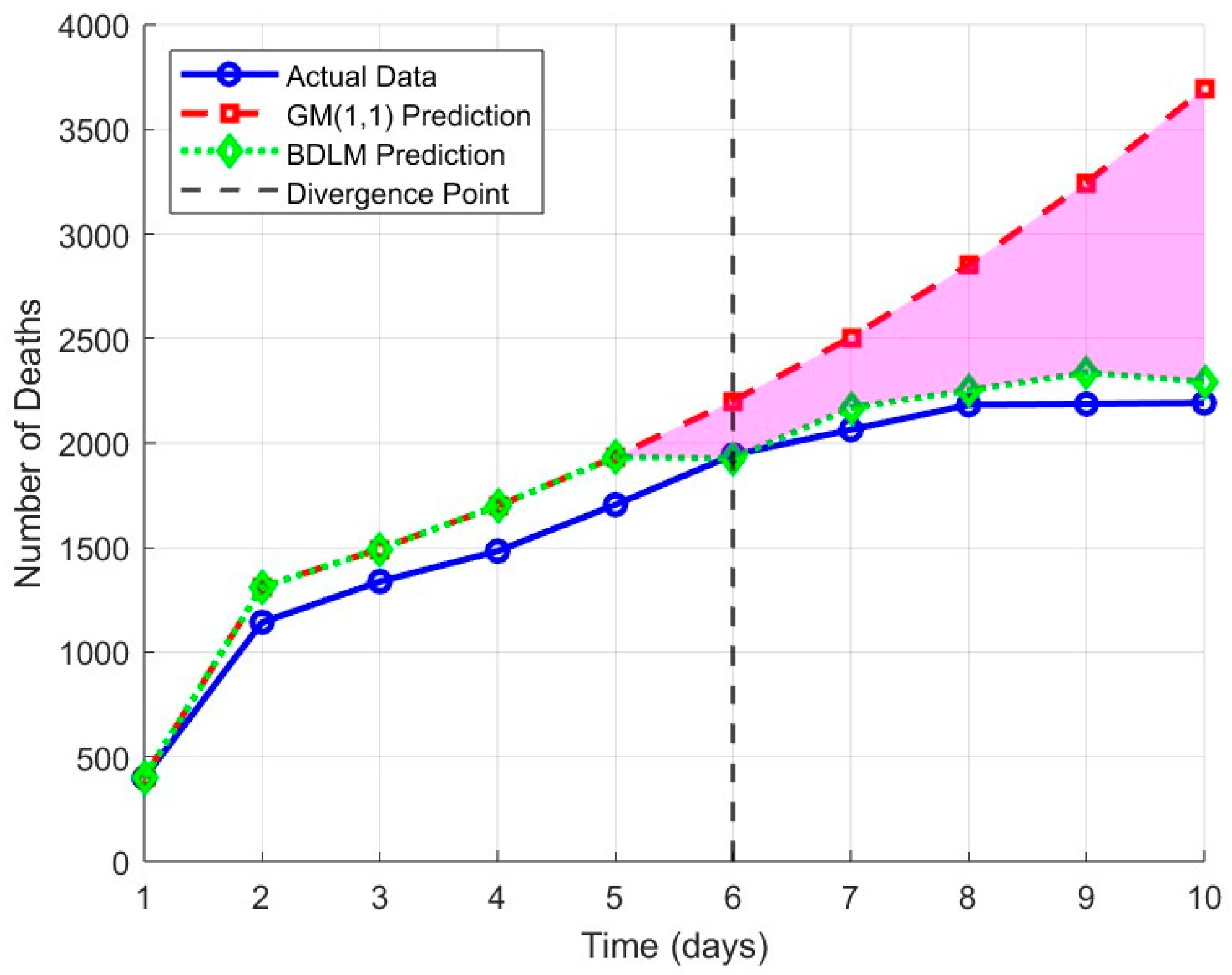
Figure 2 and

Table 2. Comparison of fatality counts.

Day	Actual Value	GM(1,1) Prediction	BDLM Prediction	GM(1,1) Residual	GM(1,1) Relative Error (%)	BDLM Residual	BDLM Relative Error (%)
6	1944	2202	1928	258	13.27	−16	0.82
7	2064	2505	2170	441	21.37	106	5.13
8	2183	2851	2254	668	30.60	71	3.25
9	2187	3244	2339	1057	48.33	152	6.95
10	2192	3692	2295	1500	68.43	103	4.70
Average	1664.30	2133.60	1782.80	469.30	23.63		4.01

present the comparative performance of GM(1,1) and BDLM in predicting fatality counts. The results demonstrate that while GM(1,1) shows fairly accurate predictions in early stages, its forecasts progressively diverge from observed values over time. In contrast, BDLM maintains consistent accuracy throughout the forecasting period.

In contrast, the BDLM continuously incorporates new observations to dynamically update and refine its forecasts. Therefore, its predictions are more closely aligned with the evolving trends in the actual data. This advantage stems from the fact that the BDLM incorporates both a state equation and an observation equation, which jointly describe the dynamic evolution of the system. Furthermore, the Kalman filter mechanism enables real-time updating of the state estimates, thereby adapting to changes in the observed data.

On the other hand, while GM(1,1) can provide initial forecasts even with limited data availability, it lacks the capability for dynamic adjustment. Thus, by integrating the strengths of both models—the robustness of GM(1,1) in handling sparse data and the adaptability of BDLM in capturing dynamic patterns—we develop a more accurate and flexible approach for forecasting emergency material demand following earthquakes.

As demonstrated in the comparative analysis above, integrating the BDLM with the GM(1,1) provides an effective approach to addressing the uncertainty in emergency material demand and the scarcity of data during the early stages of an earthquake.

By combining these two models, the hybrid approach leverages Grey System Theory to generate reliable initial forecasts based on limited early-stage data. It then utilizes BDLMs to continuously update predictions in real time as new observations become available, thereby significantly improving forecasting accuracy and adaptability.

3.4. Emergency Material Demand Forecasting

Taking drinking water as an example, this study forecasts the demand for consumable emergency supplies during post-earthquake rescue operations based on the previously predicted number of fatalities and survivors. The key parameters used in the calculation are summarized in

Table 3. Key parameter values.

Parameter	${\mathit{a}}_{\mathit{i}}$	$\bar{\mathit{T}}$	$\mathit{\alpha }$	${\mathit{z}}_{1-\mathit{\alpha }}$
Value	2500	2	0.05	1.28

, and the forecasting results for emergency material demand are presented in

Table 4. Forecasted demand for drinking water.

Day	Fatalities	Survivors	Average Demand (L/Day)	Upper Bound of Demand (L/Day)	Potential Shortage (L)
6	1928	104,976	524,880	527,140	2260
7	2170	104,734	523,670	526,083	2413
8	2254	104,650	523,250	525,877	2627
9	2339	104,565	522,825	525,574	2749
10	2295	104,609	523,045	525,876	2831

.

As shown in Table 4, the demand for emergency materials—using drinking water as an illustrative example—is forecasted for Days 6 to 10 following the large-scale earthquake. By adjusting the parameter values in Table 3, this model can be applied to other types of critical emergency supplies such as tents, food, lighting equipment, and medical supplies.

From the results, it can be observed that in order to ensure sufficient supplies for disaster victims before the next batch of relief goods arrives, each delivery should meet the average demand over the maximum waiting period plus an additional buffer to account for forecast uncertainty (i.e., potential supply shortages). This ensures both operational reliability and resilience in emergency logistics planning.

4. Discussion

The proposed GM(1,1)-BDLM hybrid forecasting framework significantly improves early-stage disaster response forecasting, particularly under conditions of data scarcity and high uncertainty. Similarly to prior enhancements of grey models—such as the Metabolism Grey–Markov approach [25] and the inventory-integrated GM(1,1)—our model aims to boost forecasting accuracy. All three models share the foundational use of GM(1,1) to capture nonlinear trends in small-sample settings, and each incorporates complementary techniques to improve adaptability. However, unlike these static or structurally improved models, the hybrid framework integrates BDLMs with Kalman filtering, enabling real-time updates as new data emerge. This dynamic adaptability resulted in an impressive average relative error of just 4.01% in the 2010 Yushu Earthquake case study. Furthermore, while prior models focus mainly on flood scenarios, this study extends grey-based forecasting to sudden-onset seismic events and incorporates multi-category resource demand, enhancing operational relevance. Overall, the framework advances traditional grey models by introducing real-time responsiveness, broader disaster applicability, and stronger support for emergency logistics planning.

5. Conclusions

The hybrid GM(1,1)-BDLM framework demonstrates three significant advantages: (1) It achieves superior forecasting accuracy with a 4.01% prediction error for days 6–10, representing a 19.62-percentage-point improvement over standalone GM(1,1). (2) The novel two-phase methodology effectively combines GM(1,1)’s small-sample capability with BDLM’s real-time updating, as validated in the 2010 Yushu earthquake case study. (3) The system provides operational decision support for multi-category resource allocation (water, food, medical supplies), significantly improving early-stage disaster response efficiency.

The study has two main limitations: the BDLM’s dependency on historical data patterns may limit performance in unprecedented scenarios, and the current framework lacks the integration of emerging data sources like social media or remote sensing.

Future research should focus on integrating non-traditional real-time data sources, developing meta-learning approaches for regional adaptation, and implementing multi-agent simulation for policy assessment.

This framework provides an effective solution for emergency material allocation, with its balanced accuracy and adaptability offering valuable support for disaster response decision-making. Further validation across diverse disaster cases will strengthen its practical applicability.