


Mapping Spatial Interconnections with Distances for Evaluating the Development Value of Eco-Tourism Resources


Abstract
1. Introduction
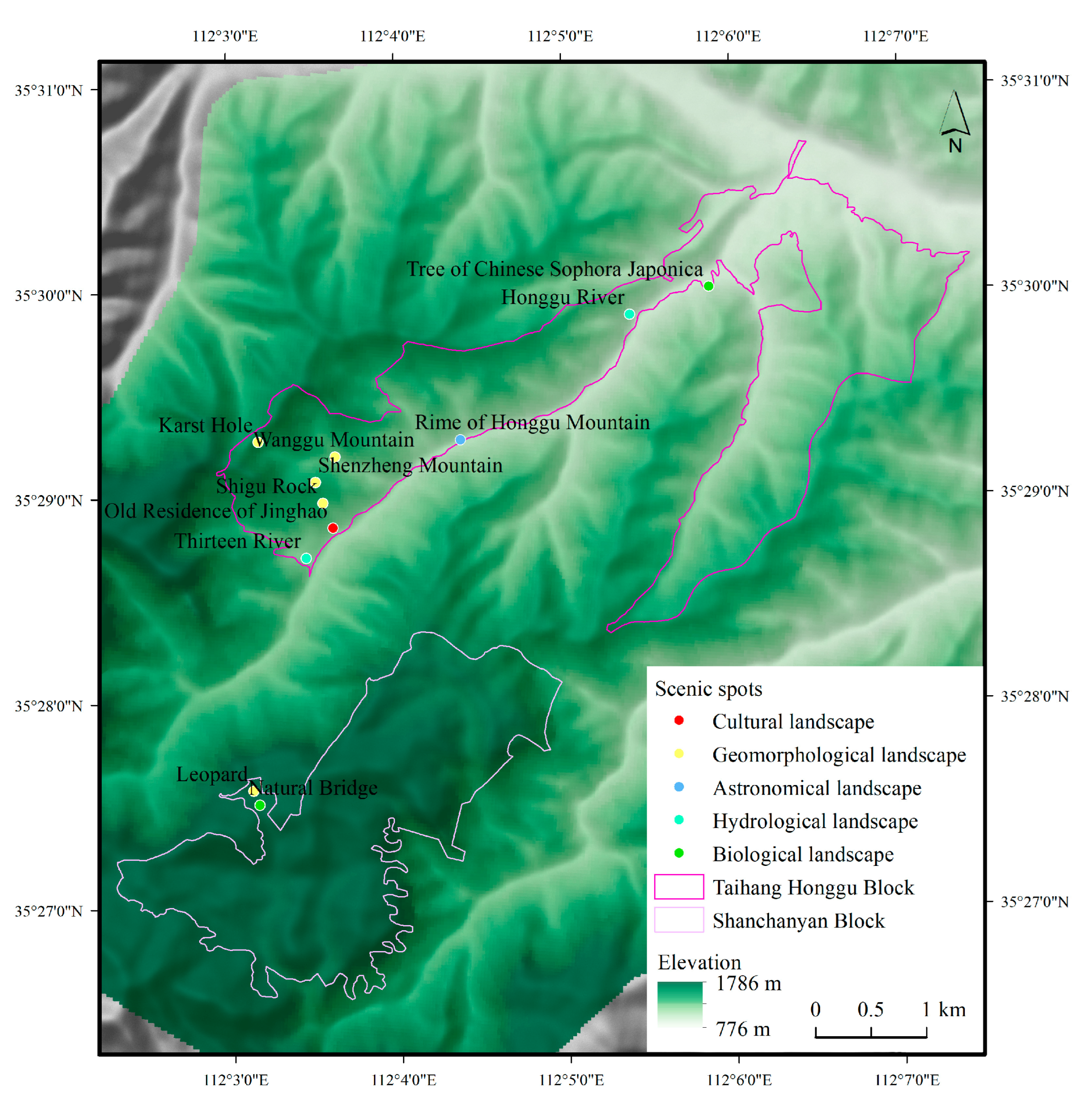
2. Study Area
3. Data and Methods
3.1. Data
3.2. Methods
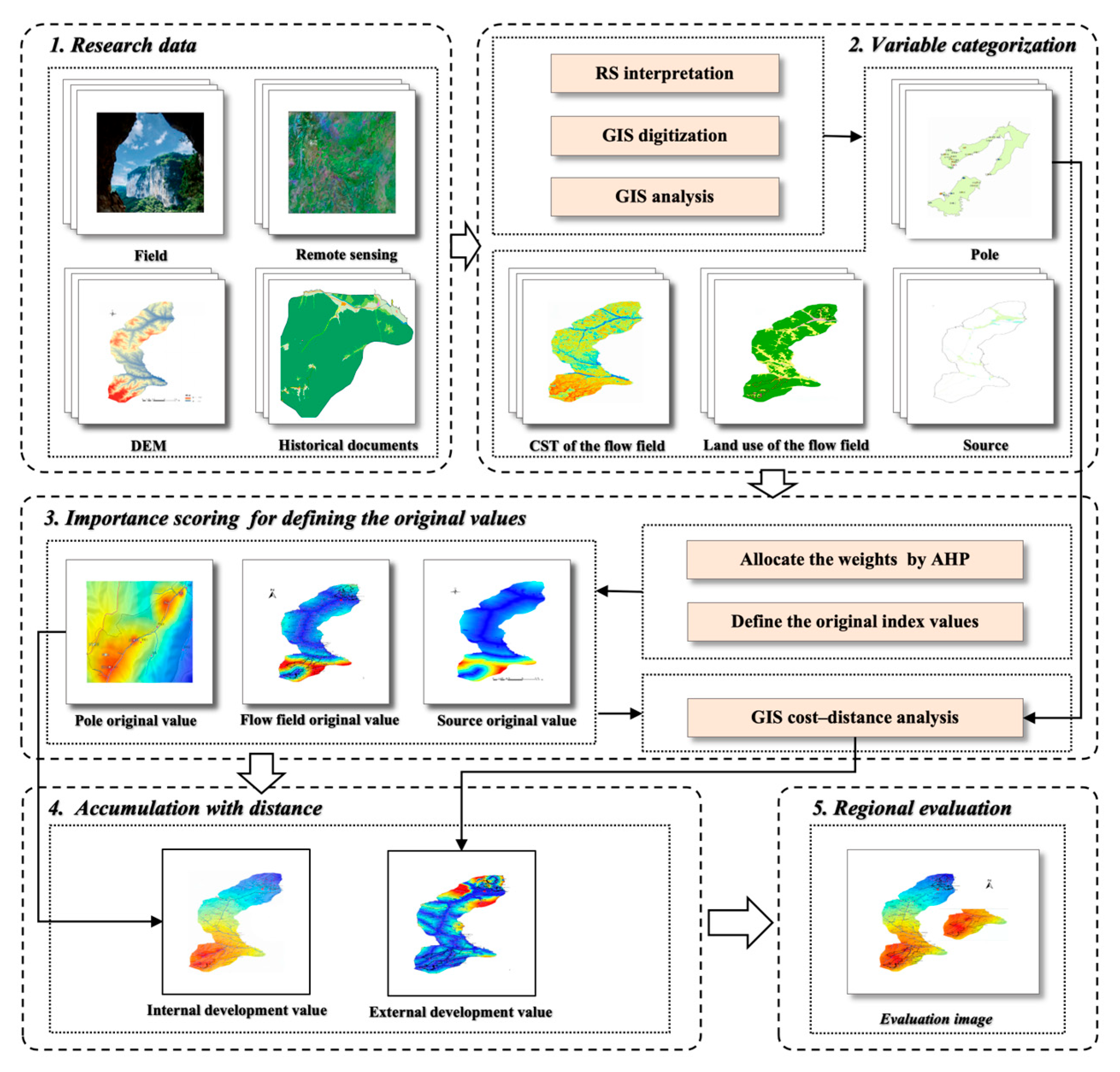
3.2.1. Methodological Framework
3.2.2. Categorization of the Evaluation Indicators
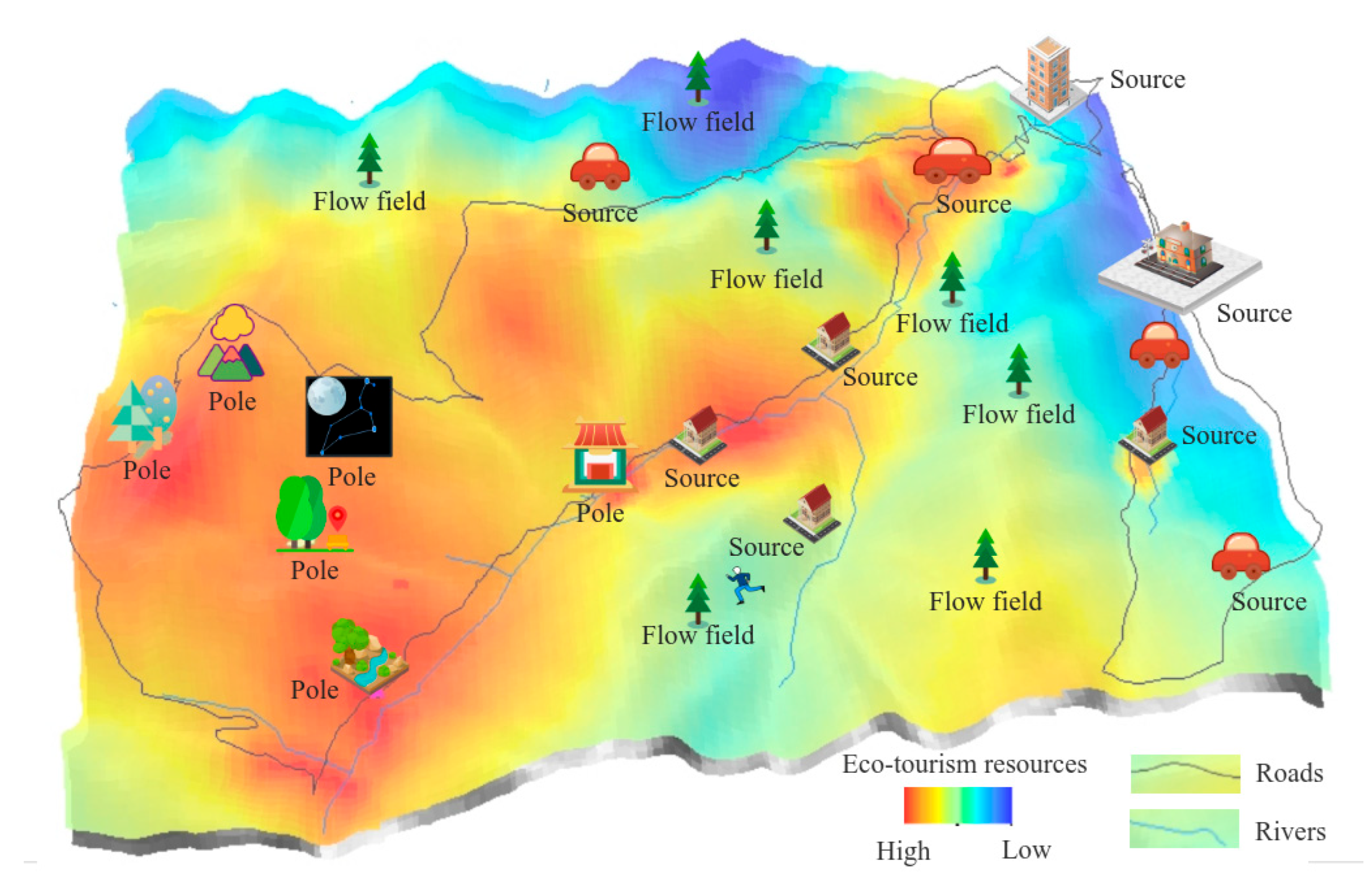
- (1)
- Pole
- (2)
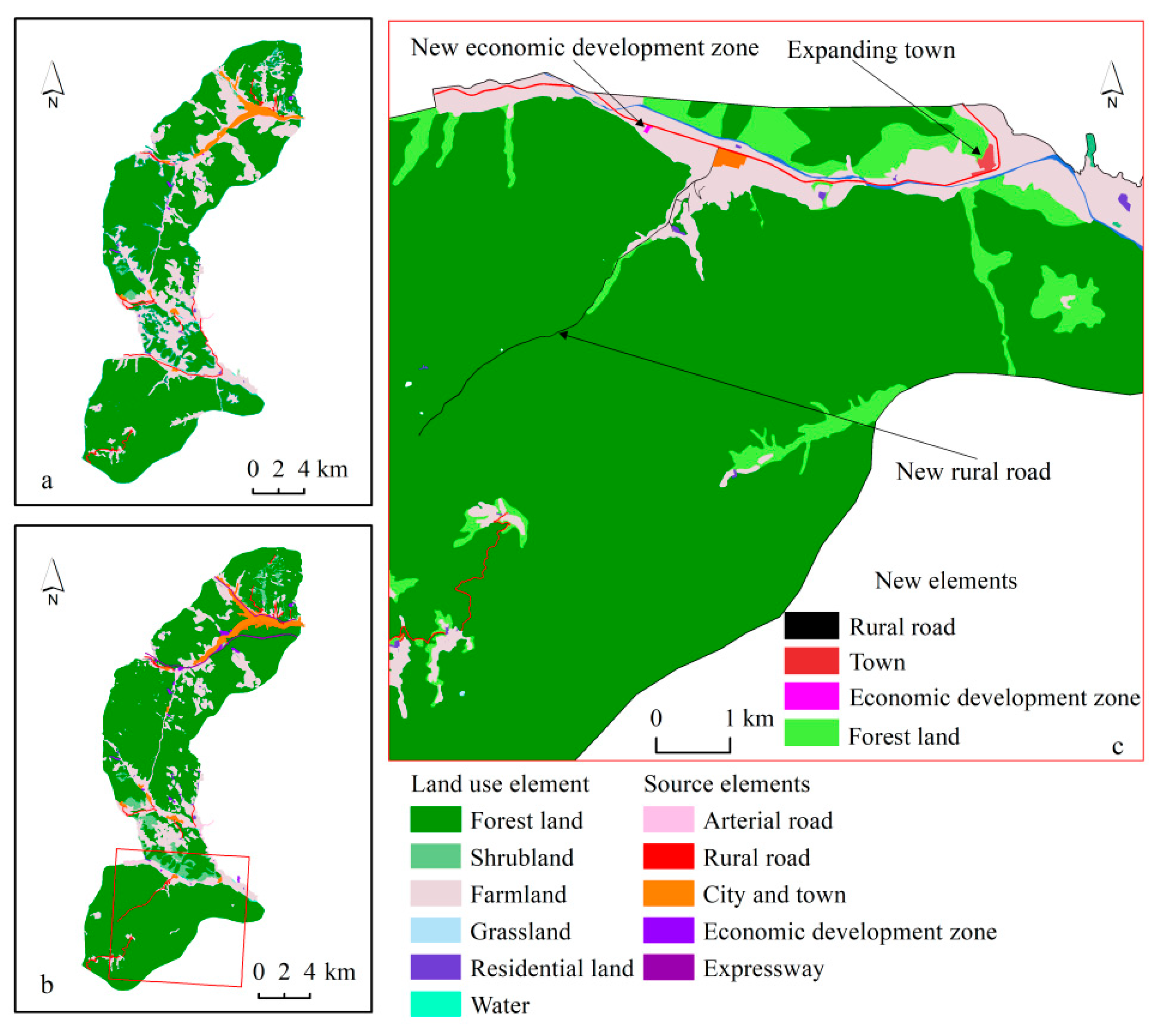
- Source
- (3)
- Flow Field
3.2.3. Scoring the Importance of the Elements of the Evaluation Indicators
3.2.4. Weight Calculation for the Evaluation Elements of the Three Indicators
3.2.5. Definition of the Initial Index Value for Evaluation Elements
3.2.6. Accumulation of the Development Value for Evaluation Mapping
4. Results
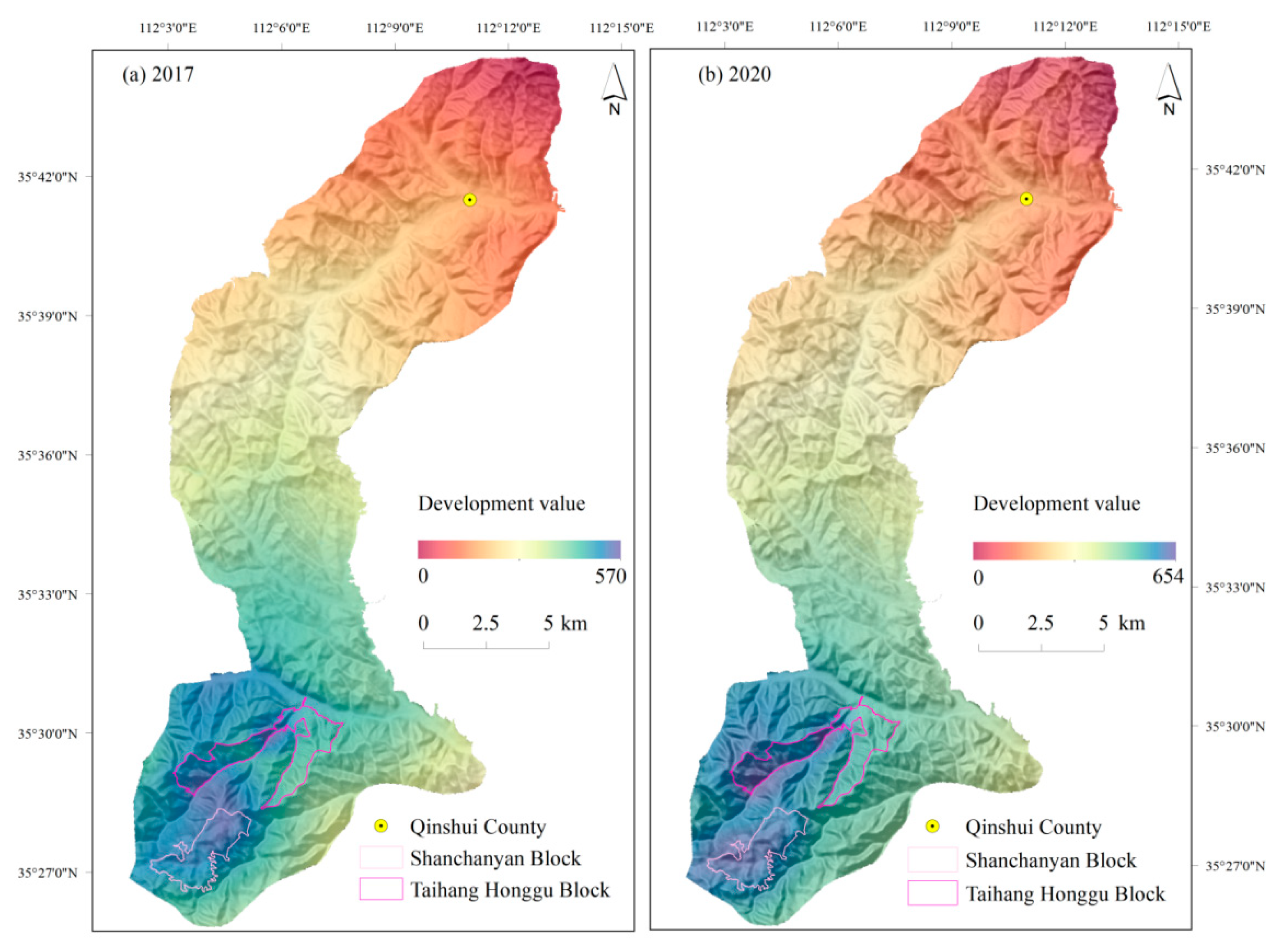
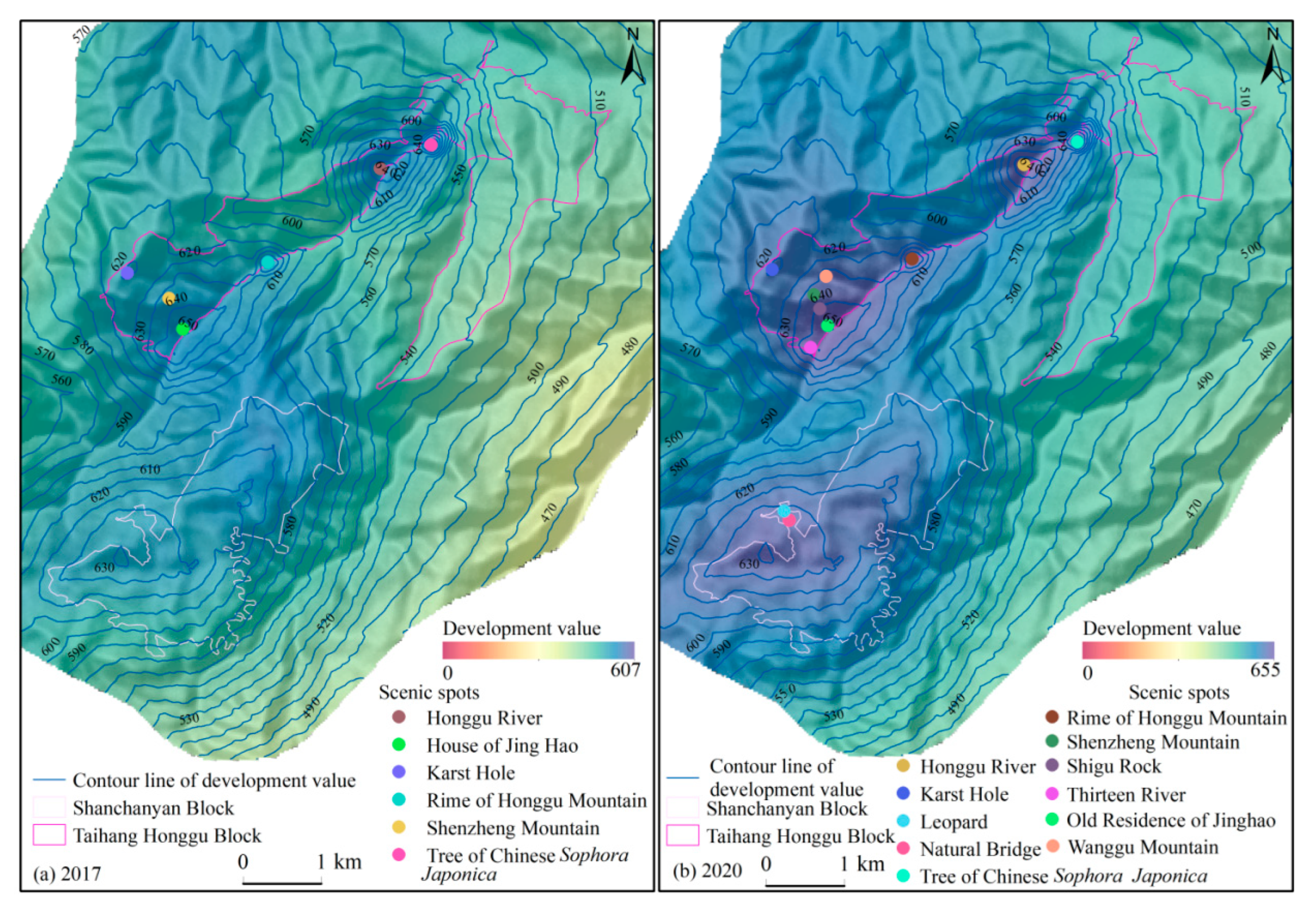
4.1. Mapping of Eco-Tourism Development Value
4.2. Effects of the Evaluation Indicators
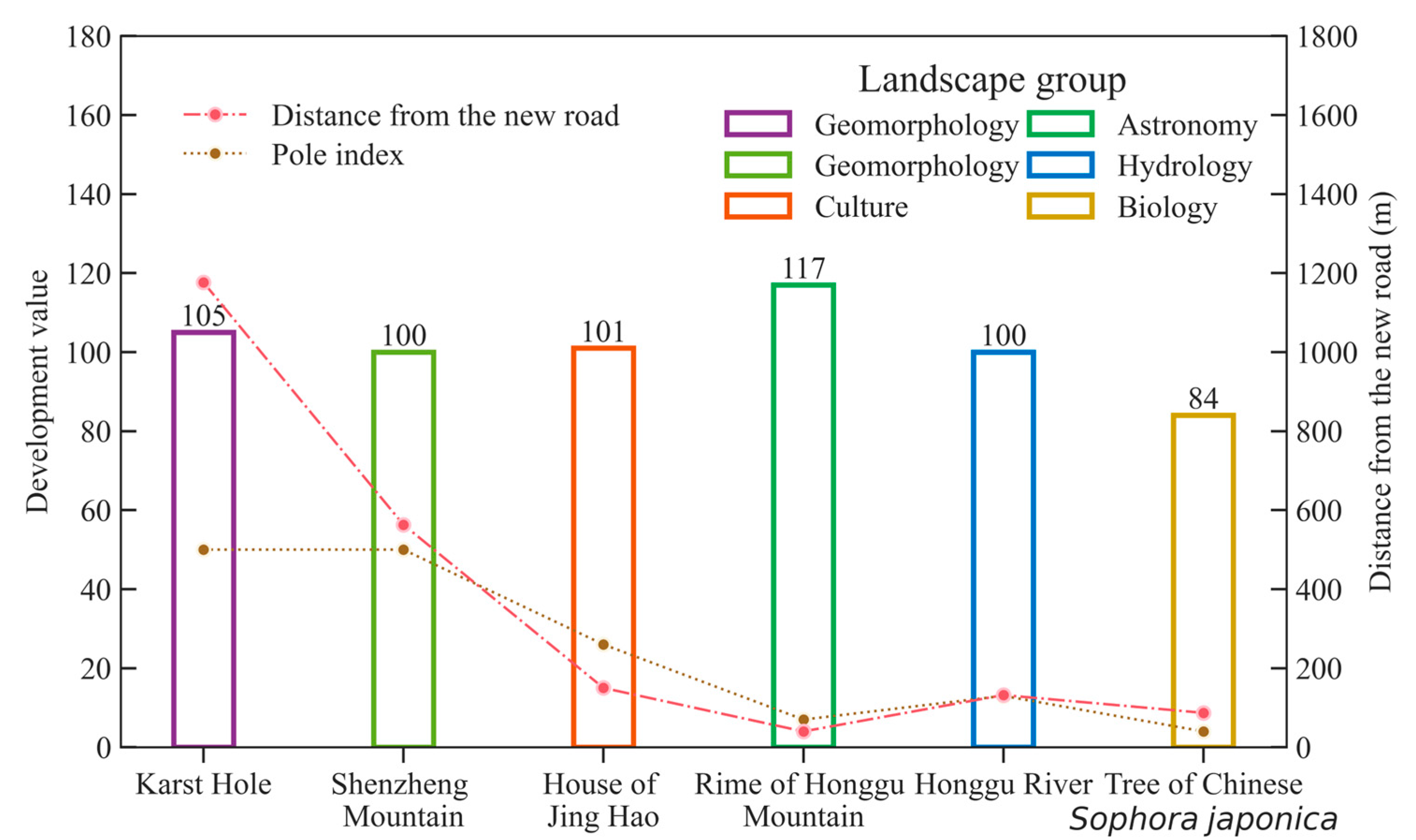
4.2.1. Pole
4.2.2. Source
4.2.3. Flow Field
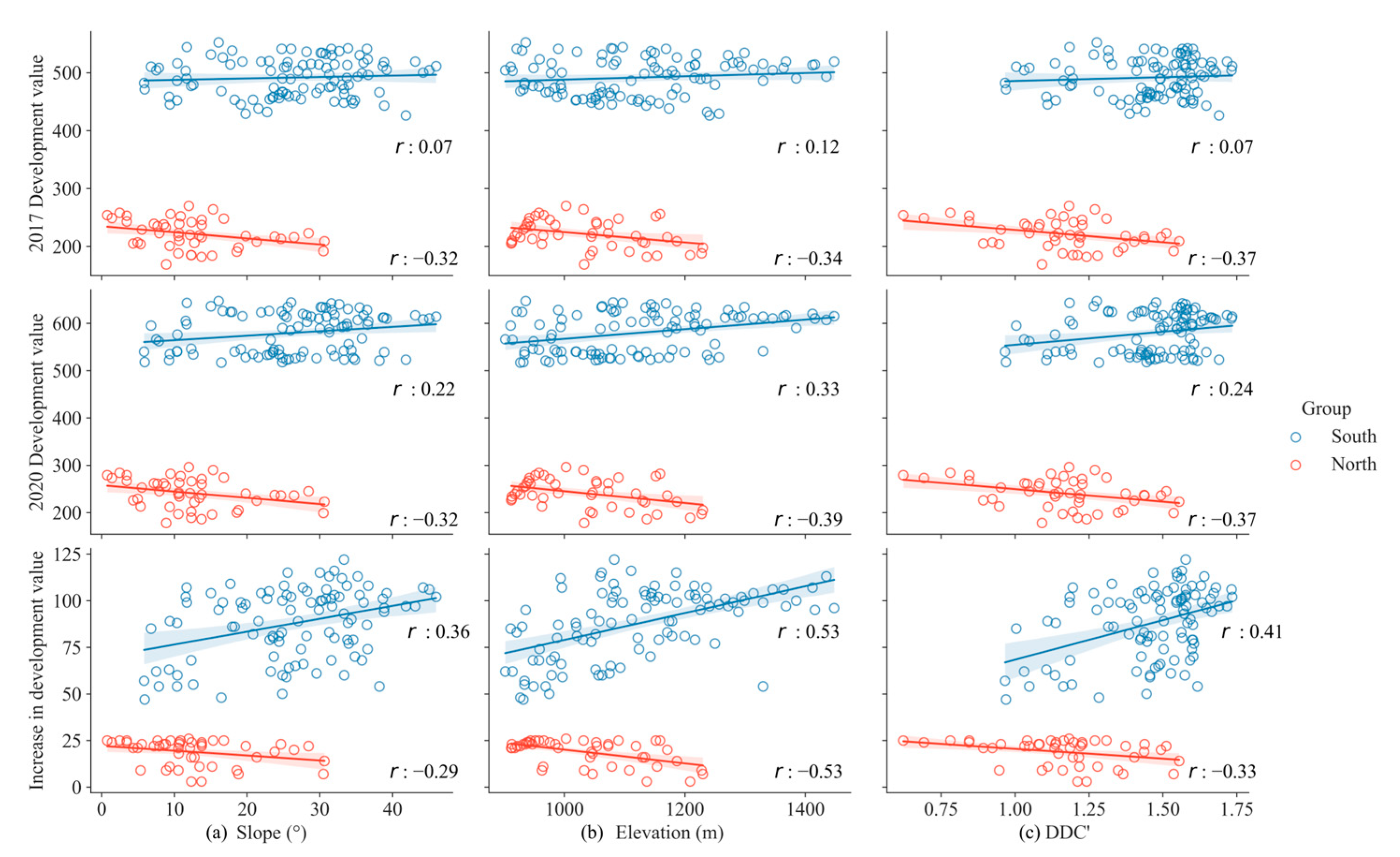
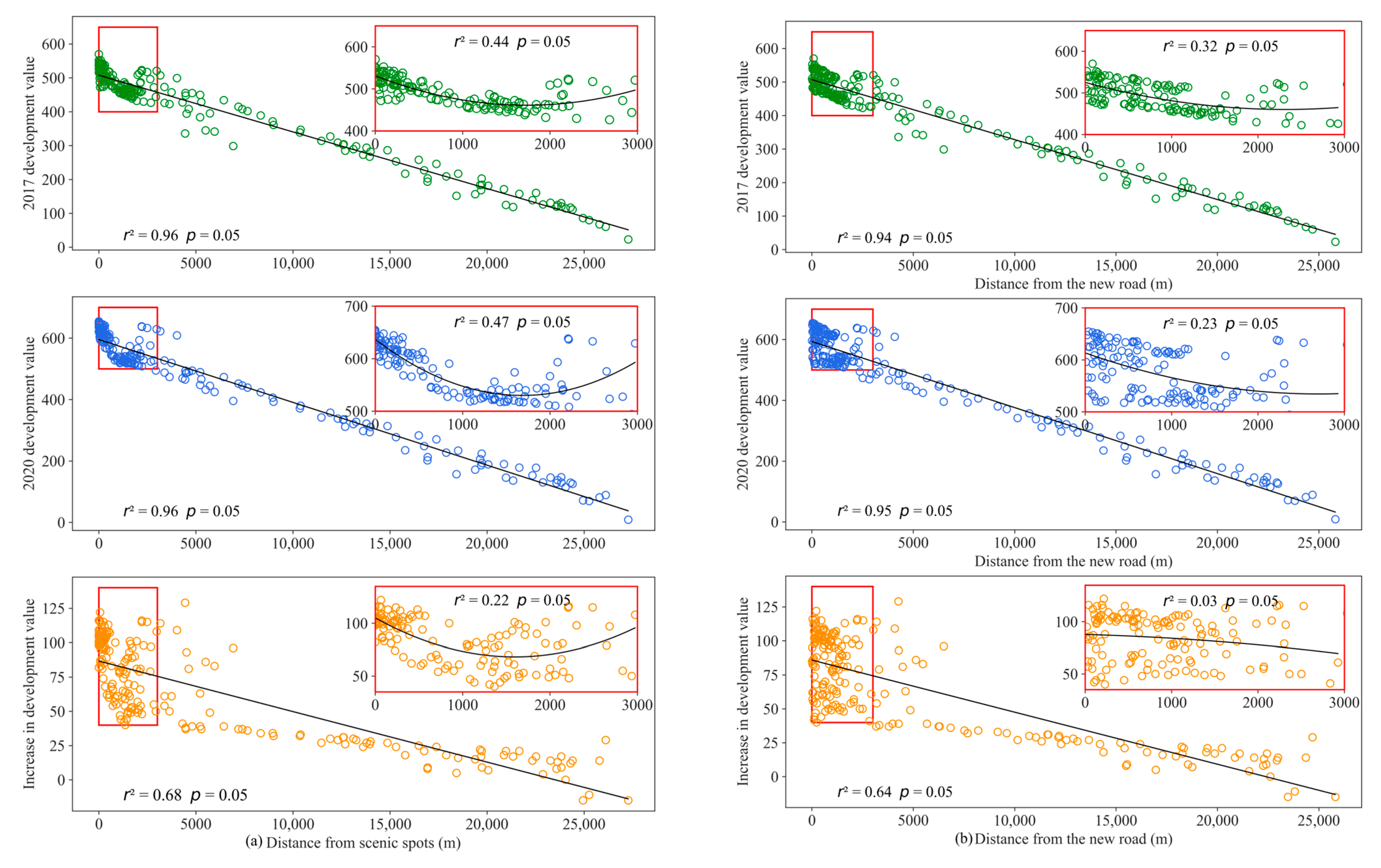
4.2.4. Spatial Distance
5. Discussion
5.1. Effectiveness of the Presented GIS Approach in a Regional Evaluation
5.2. Interpretation of Variables’ Influences on the Evaluation
5.3. Authenticity Test Using Contemporary Land Prices
5.4. Clarification of the Relationship Between Conventional Understanding and This Study
5.5. Uncertainty and Limitations
6. Conclusions
Author Contributions
Funding
Institutional Review Board Statement
Informed Consent Statement
Data Availability Statement
Conflicts of Interest
References
- Pan, X.F.; Rasouli, S.; Timmermans, H. Investigating tourist destination choice: Effect of destination image from social network members. Tour. Manag. 2021, 83, 104217. [Google Scholar] [CrossRef]
- Ng, S.L. Bibliometric analysis of literature on mountain tourism in Scopus. J. Outdoor Rec. Tour. 2022, 40, 100587. [Google Scholar] [CrossRef]
- Jeelani, P.; Shah, S.A.; Dar, S.N.; Rashid, H. Sustainability constructs of mountain tourism development: The evaluation of stakeholders’ perception using SUS-TAS. Environ. Dev. Sustain. 2023, 25, 8299–8317. [Google Scholar] [CrossRef]
- Sezerel, H.; Karagoz, D. The challenges of sustainable tourism development in special environmental protected areas: Local resident perceptions in Datça–Bozburun. Sustainability 2023, 15, 3364. [Google Scholar] [CrossRef]
- Dong, W.; Wu, X.; Zhang, J.J.; Zhang, Y.L.; Dang, H.; Lü, Y.H.; Wang, C.; Guo, J.Y. Spatiotemporal heterogeneity and driving factors of ecosystem service relationships and bundles in a typical agropastoral ecotone. Ecol. Indic. 2023, 156, 111074. [Google Scholar] [CrossRef]
- González-Rodríguez, M.R.; Díaz-Fernández, M.C.; Pulido-Pavón, N. Tourist destination competitiveness: An international approach through the travel and tourism competitiveness index. Tour. Manag. Perspect. 2023, 47, 101127. [Google Scholar] [CrossRef]
- Rubita, I. Sustainability issue in tourism: A case study of Yuksam Village, Sikkim. ATNA J. Tour. Stud. 2012, 7, 117–129. [Google Scholar] [CrossRef]
- Chakraborty, S.; Chakma, N. Perspective on large cardamom cultivation and its challenges in West Sikkim, India. Space Cult. India 2019, 6, 189–197. [Google Scholar] [CrossRef]
- Verma, T.; Rebelo, L.; Araújo, N.A.M. Impact of inter-country distances on international tourism. PLoS ONE 2019, 14, e0225315. [Google Scholar] [CrossRef]
- Li, C.; He, L.; Guo, W.; Wang, K.; Tang, S. A study on the influence of perceived distance on China’s inbound tourism and the interaction of non-economic distance: An analysis of dynamic extended gravity model based on 61 countries’ entry data (2004–2018). PLoS ONE 2024, 19, e0297442. [Google Scholar] [CrossRef]
- Ren, C.; Jóhannesson, G.T.; Ásgeirsson, M.H.; Woodall, S.; Reigner, N. Rethinking connectivity in Arctic tourism development. Ann. Tour. Res. 2024, 105, 103705. [Google Scholar] [CrossRef]
- Chakraborty, P.; Ghosal, S. An eco-social exploration of tourism area evolution in mountains through stakeholders’ perspective. Environ. Dev. 2024, 49, 100963. [Google Scholar] [CrossRef]
- Shao, Y.; Liu, Y.; Li, Y.; Yuan, X. Regional ecosystem services relationships and their potential driving factors in the Yellow River Basin, China. J. Geogr. Sci. 2023, 33, 863–884. [Google Scholar] [CrossRef]
- Darko, A.; Chan, A.P.C.; Ameyaw, E.E.; Owusu, E.K.; Pärn, E.; Edwards, D.J. Review of application of analytic hierarchy process (AHP) in construction. Int. J. Constru. Manag. 2019, 19, 436–452. [Google Scholar] [CrossRef]
- Saaty, T.L. Decision Making for Leaders: The Analytical Hierarchy Process for Decisions in a Complex World. In Lifetime Learning Publications; RWS Publications: Pittsburgh, PA, USA, 1982; ISBN 534-97959-9. [Google Scholar]
- Chakraborty, P.; Ghosal, S. Status of mountain-tourism and research in the Indian Himalayan Region: A systematic review. Asia-Pac. J. Reg. Sci. 2022, 6, 863–897. [Google Scholar] [CrossRef]
- Mutaganda, T.; Bizimana, J.P. Application of geospatial techniques for monitoring Gikondo wetland management: From industrial park to eco-tourism park. Int. J. Environ. Agric. Res. 2020, 6, 30–35. [Google Scholar]
- He, Z.; Shang, X.; Zhang, T.; Yun, J. Coupled regulatory mechanisms and synergy trade-off strategies of human activity and climate change on ecosystem service value in the loess hilly fragile region of northern Shaanxi, China. Ecol. Indic. 2022, 143, 109325. [Google Scholar] [CrossRef]
- Marzuki, A.; Bagheri, M.; Ahmad, A.; Masron, T.; Akhir, M.F. Establishing a GIS-SMCDA model of sustainable eco-tourism development in Pahang, Malaysia. Episodes 2023, 46, 375–387. [Google Scholar] [CrossRef]
- Grêt-Regamey, A.; Bebi, P.; Bishop, I.D.; Schmid, W.A. Linking GIS-based models to value ecosystem services in an alpine region. J. Environ. Manag. 2008, 89, 197–208. [Google Scholar] [CrossRef]
- Greenberg, J.A.; Rueda, C.; Hestir, E.L.; Santos, M.J.; Ustin, S.L. Least cost distance anaylsis for spatial interpolation. Comput. Geosci. 2011, 37, 272–276. [Google Scholar] [CrossRef]
- Liu, Q.F.; Long, X.M.; Deng, Z.J.; Ye, J.X. Application of unmanned aerial vehicle in quick construction of visual scenes for national forest parks. For. Resour. Manag. 2019, 28, 116–122. [Google Scholar] [CrossRef]
- Düzgüneş, E.; Demirel, Ö. Determining the tourism potential of the Altındere Valley National Park (Trabzon/Turkey) with respect to its conservation value. Int. J. Sustain. Dev. World Ecol. 2013, 20, 358–368. [Google Scholar] [CrossRef]
- Zhang, Y. A model and its application of quantitative evaluation for exploitable value of hot spring landscape resources. Math. Probl. Eng. 2022, 2022, 6859092. [Google Scholar] [CrossRef]
- Zhao, Q.; Tang, H.; Gao, C.; Wei, Y. Evaluation of urban forest landscape health: A case study of the Nanguo Peach Garden, China. iForest 2020, 138, 175–184. [Google Scholar] [CrossRef]
- GB/T18005-1999; National Public Service Platform for Standards Information, China Forest Park Landscape Resource Grade Evaluation. National Forestry and Grassland Administration: Beijing, China, 2000. Available online: https://openstd.samr.gov.cn/bzgk/std/newGbInfo?hcno=D19B825BBFB3C851215F178B2A3CE4E7 (accessed on 1 July 2025).
- Nugroho, P.; Numata, S. Resident support of community-based tourism development: Evidence from Gunung Ciremai National Park, Indonesia. J. Sustain. Tour. 2022, 30, 510–2525. [Google Scholar] [CrossRef]
- Pramanik, S.A.K.; Rahman, M.Z. Influences of local community dimensions in enhancing support for sustainable tourism development. Int. J. Hosp. Tour. Adm. 2024, 25, 817–841. [Google Scholar] [CrossRef]
- Zhang, X.; Luo, Y.; Wang, G.; Tian, B. Study on the design of slow travel system of tourist highway service facilities. IOP Conf. Ser. Mater. Sci. Eng. 2020, 780, 062026. [Google Scholar] [CrossRef]
- Tang, W.Y. The characteristics of urban residents’ place attachment to recreational block: A case study of Nanjing Confucius temple block. Sci. Geogr. Sin. 2011, 31, 1202–1207. [Google Scholar]
- Pearce, D.G. Towards a geography of tourism. Ann. Tour. Res. 1979, 9, 245–272. [Google Scholar] [CrossRef]
- Mitchell, L.S.; Murphy, P.E. Geography and tourism. Ann. Tour. Res. 1991, 18, 57–70. [Google Scholar] [CrossRef]
- Boavida-Portugal, I.; Rocha, J.; Ferreira, C.C. Exploring the impacts of future tourism development on land use/cover changes. Appl. Geogr. 2016, 77, 82–91. [Google Scholar] [CrossRef]
- Zhang, S.; Zhang, G.; Ju, H. The spatial pattern and influencing factors of tourism development in the Yellow River Basin of China. PLoS ONE 2020, 15, e0242029. [Google Scholar] [CrossRef]
- Lundmark, L.; Stjernström, O. Environmental protection: An instrument for regional development? National ambitions versus local realities in the case of tourism. Scand. J. Hosp. Tour. 2009, 9, 387–405. [Google Scholar] [CrossRef]
- Roth, B.J.; Howie, R.A. Land-use planning and natural resource rights: The Alberta land stewardship. J. Energy Nat. Resour. Law 2011, 29, 471–498. [Google Scholar] [CrossRef]
- Franek, J.; Kresta, A. Judgment scales and consistency measure in AHP. Procedia Econ. Financ. 2014, 12, 164–173. [Google Scholar] [CrossRef]
- Ye, J.X.; Wu, M.S.; Deng, Z.J.; Xu, S.J.; Zhou, R.L.; Clarke, K.C. Modeling the spatial patterns of human wildfire ignition in Yunnan Province, China. Appl. Geogr. 2017, 89, 150–162. [Google Scholar] [CrossRef]
- Sechu, G.L.; Nilsson, B.; Iversen, B.V.; Greve, M.B.; Børgesen, C.D.; Greve, M.H. A stepwise GIS approach for the delineation of river valley bottom within drainage basins using a cost distance accumulation analysis. Water 2021, 13, 827. [Google Scholar] [CrossRef]
- Liu, Y. The practical significance of “classification, survey and evaluation of tourism resources” from the perspective of tourism planning. J. Tour. 2006, 21, 8–9. [Google Scholar]
- Martinez-Alier, J.; Kallis, G.; Veuthey, S.; Walter, M.; Temper, L. Social metabolism, ecological distribution conflicts, and valuation languages. Cap. Nat. Soc. 2010, 70, 153–158. [Google Scholar] [CrossRef]
- Peng, D.; Liang, Z.; Ding, Y.; Liang, L.; Zhai, A.; Zhang, Y.; Gong, X. Spatial and temporal distribution characteristics and influencing factors of tourism eco-efficiency in the Yellow River Basin based on the geographical and temporal weighted regression model. PLoS ONE 2024, 19, e0295186. [Google Scholar] [CrossRef]
- Yang, X. Analysis of Dabie Mountain tourism industry internationalization-a case study of Huanggang in Hubei. SHS Web Conf. 2016, 25, 02019. [Google Scholar] [CrossRef]
- Ma, Y.; Li, L.; Ren, J. Coordination development research among the tourism economy-traffic condition-ecological environment in Shengnongjia forest district. Econ. Geogr. 2017, 37, 215–220. [Google Scholar] [CrossRef]
- Wu, G.M.; Guan, S.Q.; Xu, Y.H.; Chu, C.J.; Zhu, Z.M. The closer, the better? Impact of tourists’ psychological distance on their travel intention in the post-pandemic era. J. China Tour. Res. 2024, 20, 521–544. [Google Scholar] [CrossRef]
- Li, Z.H.; Zhang, H.P.; Xu, Y.S.; Fang, T.Y.; Wang, H.R.; Tang, G.A. How does cultural distance affect tourism destination choice? Evidence from the correlation between regional culture and tourism flow. Appl. Geogr. 2024, 166, 103261. [Google Scholar] [CrossRef]
- Hosany, S.; Buzova, D.; Sanz-Blas, S. The influence of place attachment, ad-evoked positive affect, and motivation on intention to visit: Imagination proclivity as a moderator. J. Travel Res. 2020, 59, 477–495. [Google Scholar] [CrossRef]
- Wittowsky, D.; Hoekveld, J.; Welsch, J.; Steier, M. Residential housing prices: Impact of housing characteristics, accessibility and neighbouring apartments–a case study of Dortmund, Germany. Urban Plan. Transp. Res. 2020, 8, 44–70. [Google Scholar] [CrossRef]
- Cong, S.; Chin, L.; Abdul Samad, A.R. Does urban tourism development impact urban housing prices. Int. J. Hous. Mark. Anal. 2025, 18, 5–24. [Google Scholar] [CrossRef]
- Herbei, M.; Nemes, I. Using GIS analysis in transportation network. Int. Multidiscip. Sci. GeoConference SGEM 2012, 2, 1193–1200. [Google Scholar]


| Indicators | Referenced Contents | Composition Elements | Type of Conditions | Role |
|---|---|---|---|---|
| Pole | Any scenic spot, referring to all the natural and cultural landscapes | Geomorphological resources, hydrological resources, biological resources, cultural resources, astronomical resources | Internal | Extremely high land prices and high Eco-TRDVs |
| Source | Sources of tourists and other sources | Distribution centers or places of origin of visitors, channels that transport tourists to scenic spots | External | Provide initial values for accumulation |
| Flow Field | Any geographical unit or potential route | Land uses, geographical factors | External | Determine investment difficulties and costs |
| Evaluation Indicator | Scoring Basis |
|---|---|
| Pole | Criteria or standards of tourism resource classification and experts’ experience |
| Source | Statistical reports of the tourism industry released by authorities and experts’ experience |
| Flow field | Local policies of current natural resource protection and utilization, as well as compensation standards for expropriation or requisition for non-freehold estates during the evaluation period |
| Element | Biological Landscape | Astronomical Landscape | Hydrological Landscape | Cultural Landscape | Geomorphological Landscape | Weight |
|---|---|---|---|---|---|---|
| Biological landscape | 1 | 3 | 5 | 7 | 9 | 0.035 |
| Astronomical landscape | 0.333 | 1 | 3 | 5 | 7 | 0.068 |
| Hydrological landscape | 0.200 | 0.333 | 1 | 3 | 5 | 0.134 |
| Cultural landscape | 0.143 | 0.200 | 0.333 | 1 | 3 | 0.260 |
| Geomorphological landscape | 0.111 | 0.143 | 0.200 | 0.333 | 1 | 0.503 |
| Element | Economic Development Zones | Cities and Towns | Rural Roads | Expressways | Arterial Roads | Weight |
|---|---|---|---|---|---|---|
| Economic development zones | 1 | 3 | 5 | 7 | 9 | 0.035 |
| Cities and towns | 0.333 | 1 | 3 | 5 | 7 | 0.068 |
| Rural roads | 0.200 | 0.333 | 1 | 3 | 5 | 0.134 |
| Expressways | 0.143 | 0.200 | 0.333 | 1 | 3 | 0.260 |
| Arterial roads | 0.111 | 0.143 | 0.200 | 0.333 | 1 | 0.503 |
| Category | Element | Forest Land | Shrubland | Grassland | Water | Residential Land | Farm Land | Weight |
|---|---|---|---|---|---|---|---|---|
| Land use | Forest land | 1 | 3 | 4 | 5 | 7 | 9 | 0.029 |
| Shrubland | 0.333 | 1 | 3 | 4 | 5 | 7 | 0.053 | |
| Grassland | 0.250 | 0.333 | 1 | 3 | 4 | 5 | 0.091 | |
| Water | 0.200 | 0.250 | 0.333 | 1 | 3 | 4 | 0.149 | |
| Residential land | 0.143 | 0.200 | 0.250 | 0.333 | 1 | 3 | 0.248 | |
| Farmland | 0.111 | 0.143 | 0.200 | 0.250 | 0.333 | 1 | 0.430 | |
| Natural geographical factor | Altitude and slope | DDC’ | ||||||
| Indicator | Element Index | Index Value | |
|---|---|---|---|
| Pole | Biological landscape | 4 | |
| Astronomical landscape | 7 | ||
| Hydrological landscape | 13 | ||
| Cultural landscape | 26 | ||
| Geomorphological landscape | 50 | ||
| Source | Economic development zones | 4 | |
| Cities and towns | 7 | ||
| Rural roads | 13 | ||
| Expressways | 26 | ||
| Arterial roads | 50 | ||
| Flow field | Land use | Forest land | 3 |
| Shrubland | 5 | ||
| Grassland | 9 | ||
| Water | 15 | ||
| Residential land | 25 | ||
| Farmland | 43 | ||
| Natural geographical factor | Altitude and slope | 100 DDC’ | |
Disclaimer/Publisher’s Note: The statements, opinions and data contained in all publications are solely those of the individual author(s) and contributor(s) and not of MDPI and/or the editor(s). MDPI and/or the editor(s) disclaim responsibility for any injury to people or property resulting from any ideas, methods, instructions or products referred to in the content. |
© 2025 by the authors. Licensee MDPI, Basel, Switzerland. This article is an open access article distributed under the terms and conditions of the Creative Commons Attribution (CC BY) license (https://creativecommons.org/licenses/by/4.0/).
Share and Cite
Zhang, W.; Cui, H.; Huang, X.; Zhou, R.; Wang, Y. Mapping Spatial Interconnections with Distances for Evaluating the Development Value of Eco-Tourism Resources. Sustainability 2025, 17, 6430. https://doi.org/10.3390/su17146430
Zhang W, Cui H, Huang X, Zhou R, Wang Y. Mapping Spatial Interconnections with Distances for Evaluating the Development Value of Eco-Tourism Resources. Sustainability. 2025; 17(14):6430. https://doi.org/10.3390/su17146430
Chicago/Turabian StyleZhang, Wenqi, Huanfeng Cui, Xiaoyuan Huang, Ruliang Zhou, and Yanxia Wang. 2025. "Mapping Spatial Interconnections with Distances for Evaluating the Development Value of Eco-Tourism Resources" Sustainability 17, no. 14: 6430. https://doi.org/10.3390/su17146430
APA StyleZhang, W., Cui, H., Huang, X., Zhou, R., & Wang, Y. (2025). Mapping Spatial Interconnections with Distances for Evaluating the Development Value of Eco-Tourism Resources. Sustainability, 17(14), 6430. https://doi.org/10.3390/su17146430