


Interpretable Network Framework for Predicting the Spatial Distribution of Chromium in Soil


Abstract
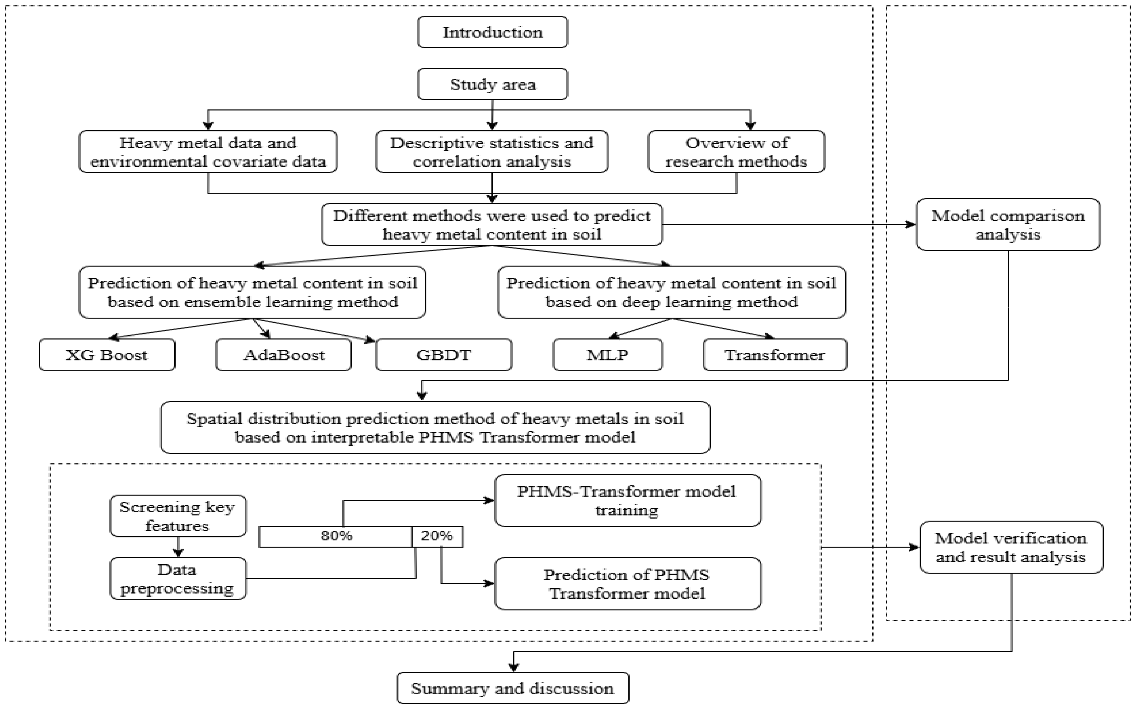
1. Introduction
2. Materials and Methods
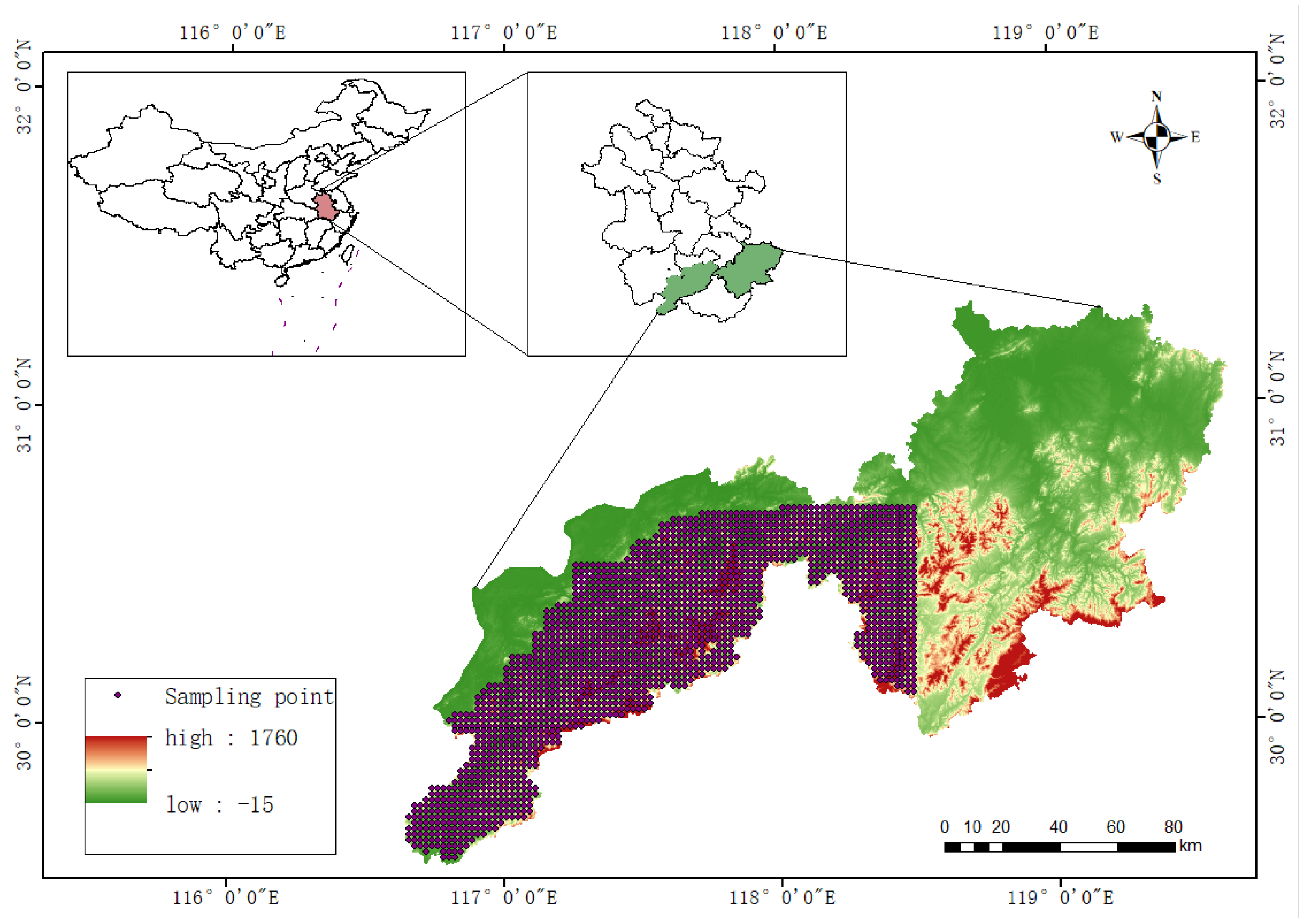
2.1. Study Area
2.2. Dataset
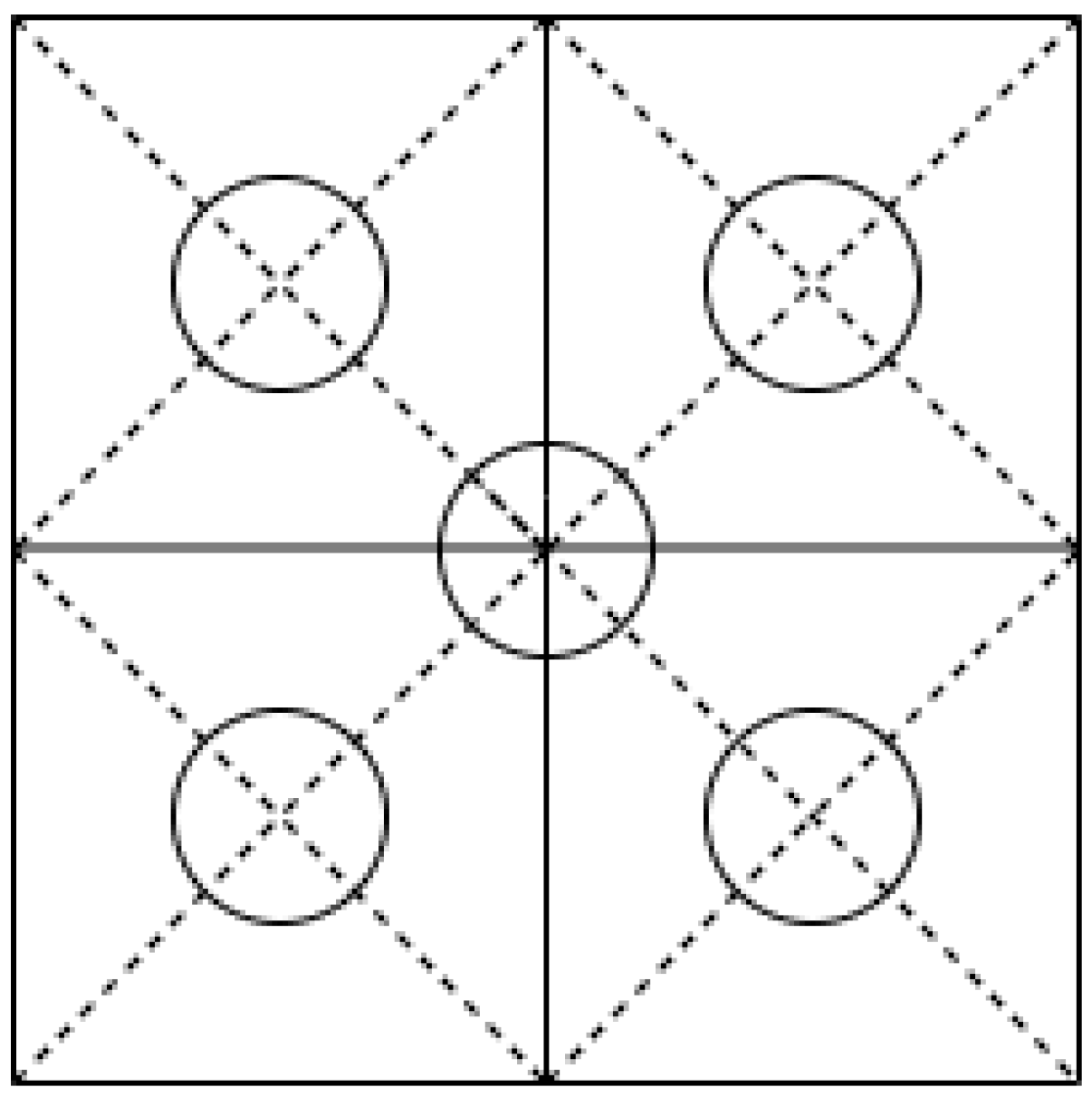
2.2.1. Soil Sampling and Chemical Analysis
2.2.2. Feature Screening
2.2.3. Environmental Data
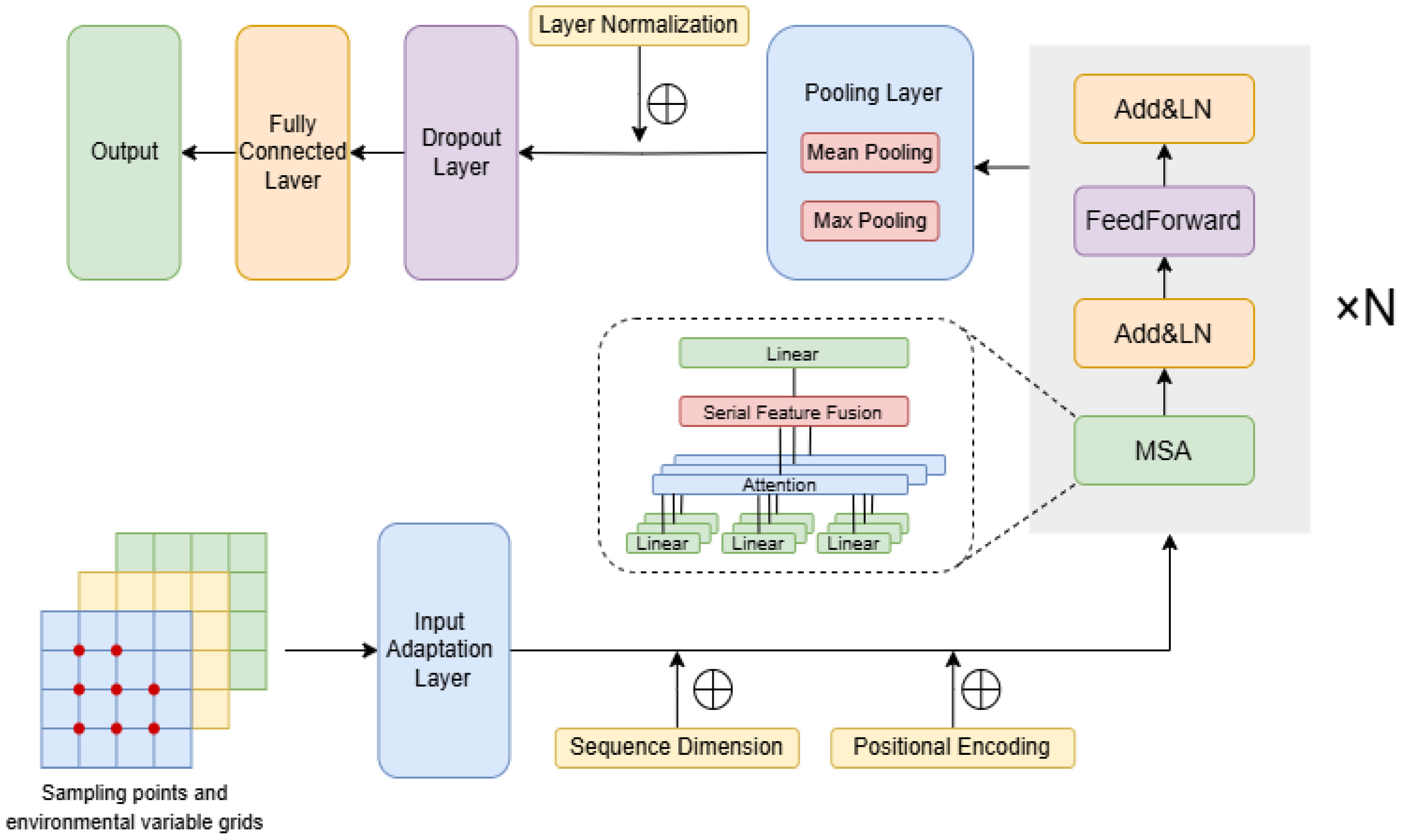
2.3. PHMS-Transformer
2.4. SHapley Additive exPlanations (SHAP)
3. Results and Discussion
3.1. Evaluation Metrics
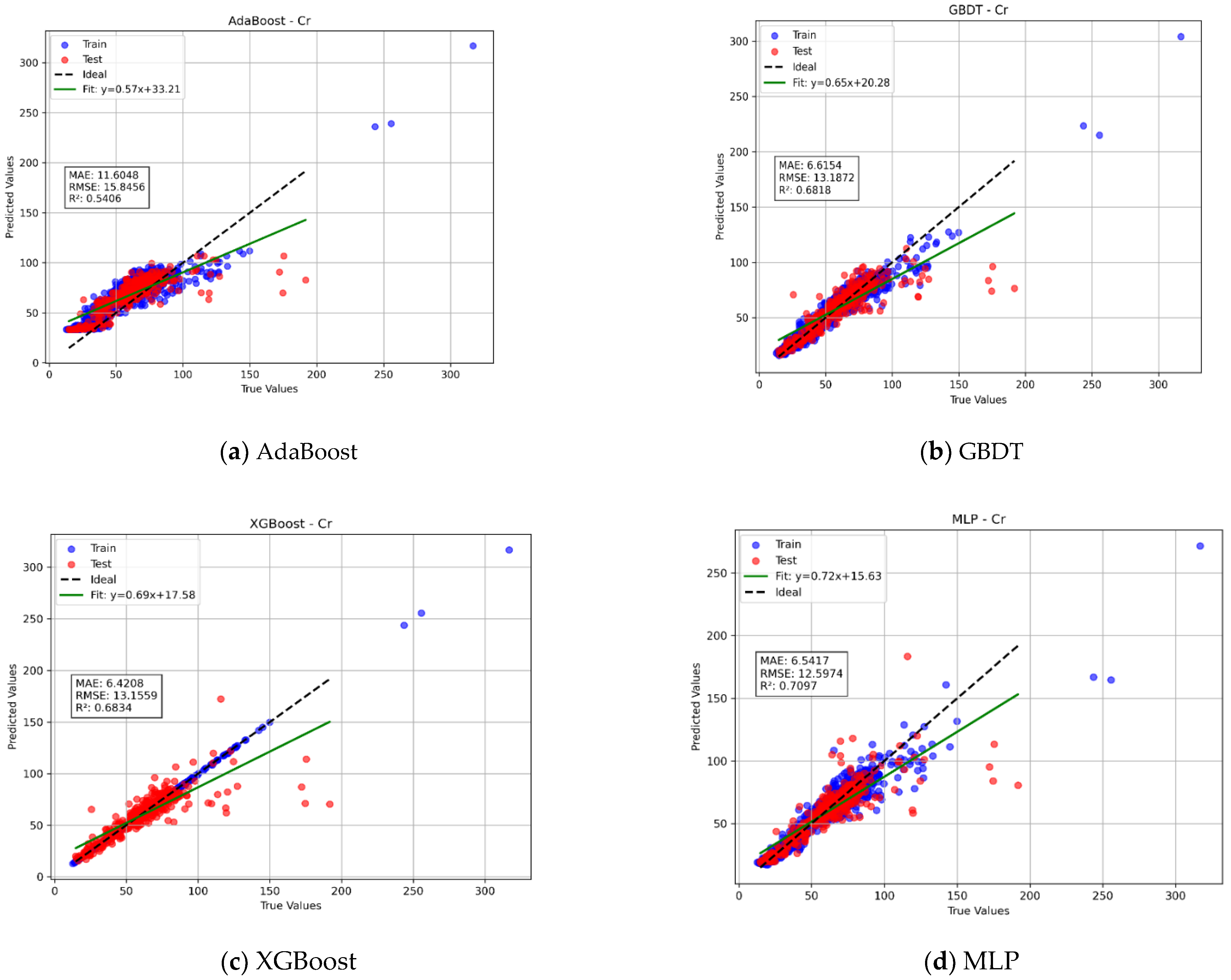
3.2. Performance Evaluation of Different Models
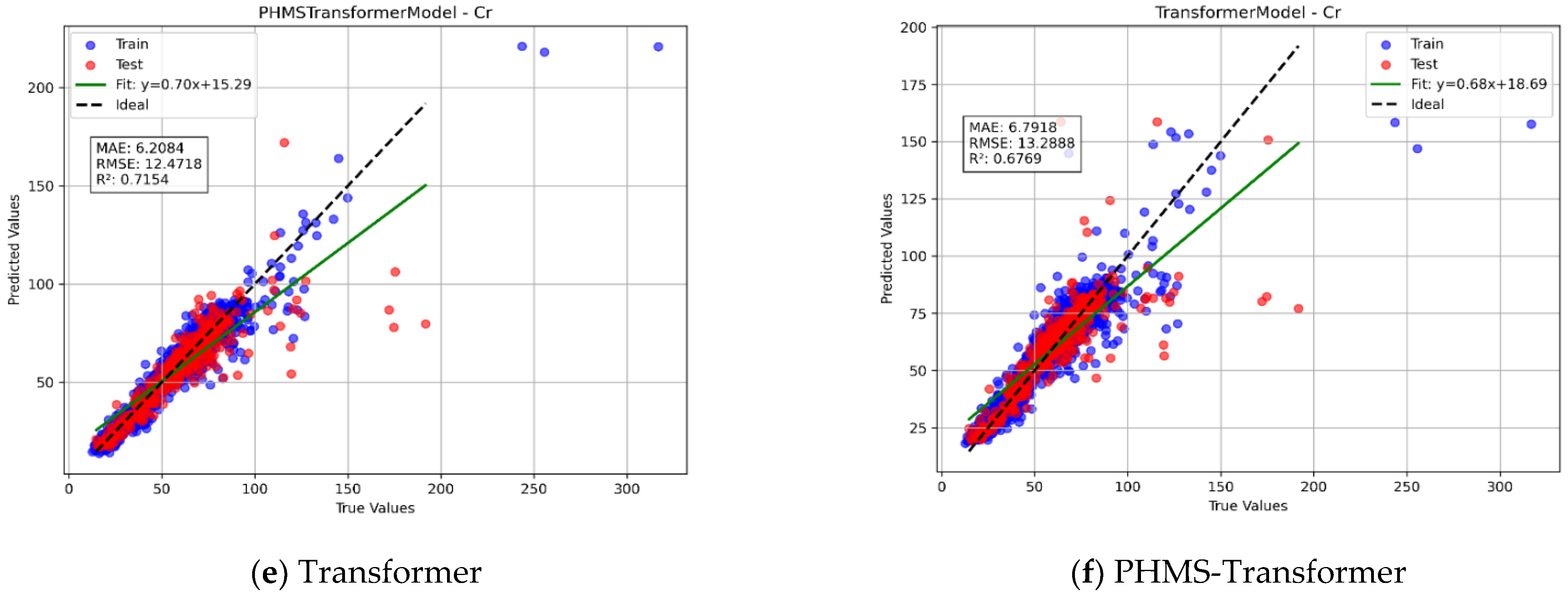
3.2.1. Comparative Analysis of Different Models for Predicting the Spatial Distribution of Heavy Metals
3.2.2. Effectiveness of Model Improvement
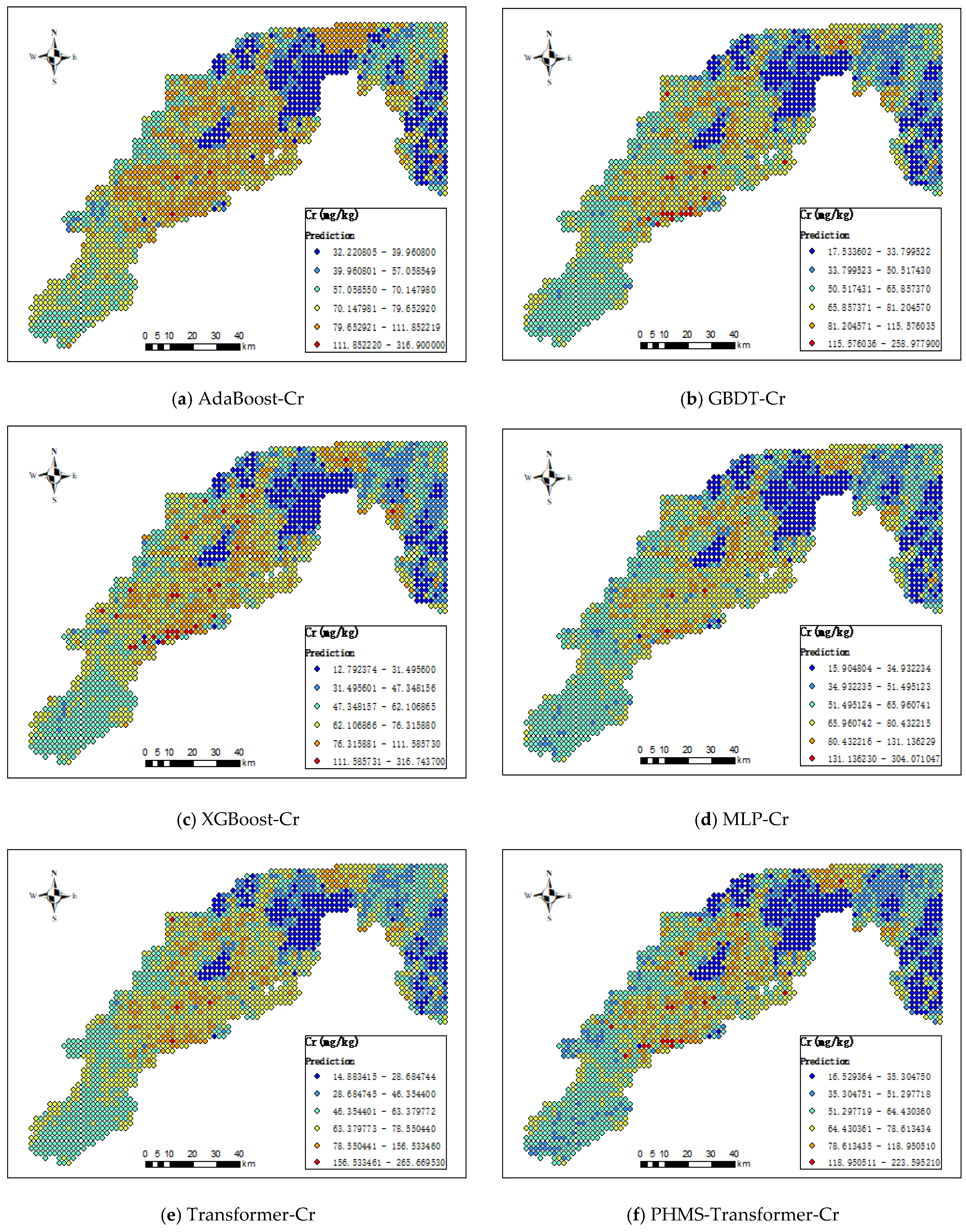
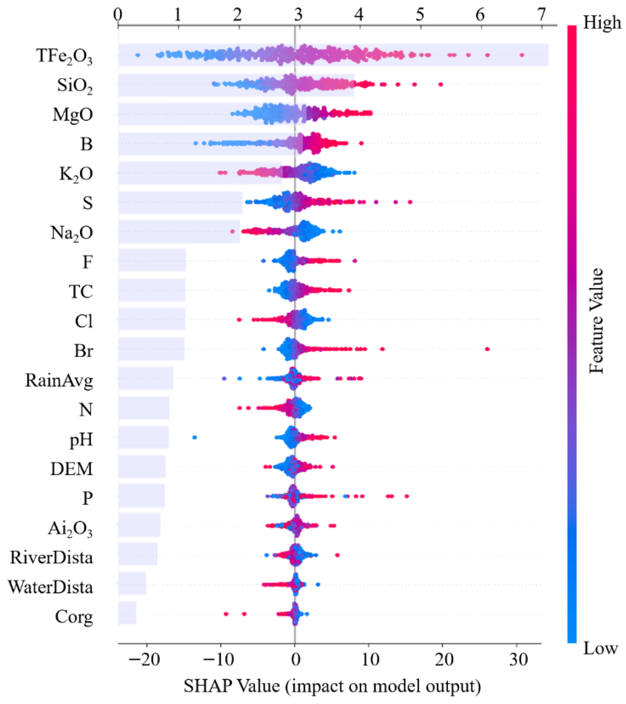
3.3. Interpretation of the Model Prediction Results
4. Conclusions
- (1)
- Regarding prediction accuracy, the PHMS-Transformer model exhibited excellent performance. Its R2 value reached 0.7182, representing a 2.7% improvement over the second-best MLP model. The MAE (6.0891) and RMSE (12.4098) decreased by 7.2% and 3.2%, respectively. Furthermore, the use of a shallow encoder and dynamic pooling strategy accelerated training by 40% while reducing overfitting risks (R2 fluctuation < 0.5%), thereby offering an efficient solution for heavy metal prediction under sparse sample conditions.
- (2)
- SHAP interpretability analysis indicated that TFe2O3 predominantly governs the spatial differentiation of Cr through adsorption and redox reactions. Additionally, topographic elevation (DEM) and river distance (RiverDista) modulate Cr migration via erosion inhibition and hydraulic transport, respectively, while pH influences Cr bioavailability by altering its chemical form. These results are consistent with geochemical theory, thereby verifying the scientific validity of the model interpretation.
Author Contributions
Funding
Institutional Review Board Statement
Informed Consent Statement
Data Availability Statement
Conflicts of Interest
References
- Zheng, X.; Lin, H.; Du, D.; Li, G.; Alam, O.; Cheng, Z.; Liu, X.; Jiang, S.; Li, J. Remediation of heavy metals polluted soil environment: A critical review on biological approaches. Ecotoxicol. Environ. Saf. 2024, 284, 116883. [Google Scholar] [CrossRef] [PubMed]
- Qiu, L.; Wang, K.; Long, W.; Wang, K.; Hu, W.; Amable, G.S. A Comparative Assessment of the Influences of Human Impacts on Soil Cd Concentrations Based on Stepwise Linear Regression, Classification and Regression Tree, and Random Forest Models. PLoS ONE 2016, 11, e0151131. [Google Scholar] [CrossRef]
- Jia, X.; O’Connor, D.; Shi, Z.; Hou, D. VIRS based detection in combination with machine learning for mapping soil pollution. Environ. Pollut. 2020, 268, 115845. [Google Scholar] [CrossRef]
- Violante, A.; Krishnamurti, G.S.R.; Pigna, M. Factors affecting the sorption-desorption of trace elements in soil environments. Biophys.-Chem. Process. Heavy Met. Met. Soil Environ. 2008, 169–214. [Google Scholar]
- Buerge, I.J.; Hug, S.J. Influence of mineral surfaces on chromium (VI) reduction by iron (II). Environ. Sci. Technol. 1999, 33, 4285–4291. [Google Scholar] [CrossRef]
- Lu, J.; Lu, H.; Brusseau, M.L.; He, L.; Gorlier, A.; Yao, T.; Tian, P.; Feng, S.; Yu, Q.; Nie, Q.; et al. Interaction of climate change, potentially toxic elements (PTEs), and topography on plant diversity and ecosystem functions in a high-altitude mountainous region of the Tibetan Plateau. Chemosphere 2021, 275, 130099. [Google Scholar] [CrossRef]
- Kowalska, J.B.; Mazurek, R.; Gąsiorek, M. Pollution indices as useful tools for the comprehensive evaluation of the degree of soil contamination—A review. Environ. Geochem. Health 2018, 40, 2395–2420. [Google Scholar] [CrossRef] [PubMed]
- Guan, Y.; Shao, C.; Ju, M. Heavy Metal Contamination Assessment and Partition for Industrial and Mining Gathering Areas. Int. J. Environ. Res. Public Health 2014, 11, 7286–7303. [Google Scholar] [CrossRef]
- Zha, Y.; Yang, Y. Innovative graph neural network approach for predicting soil heavy metal pollution in the Pearl River Basin, China. Sci. Rep. 2024, 14, 16505. [Google Scholar] [CrossRef]
- Luo, N. Methods for controlling heavy metals in environmental soils based on artificial neural networks. Sci. Rep. 2024, 14, 2563. [Google Scholar] [CrossRef]
- Santos-Francés, F.; Martínez-Graña, A.; Ávila Zarza, C.; Sánchez, A.G.; Rojo, P.A. Spatial Distribution of Heavy Metals and the Environmental Quality of Soil in the Northern Plateau of Spain by Geostatistical Methods. Int. J. Environ. Res. Public Health 2017, 14, 568. [Google Scholar] [CrossRef]
- Taghizadeh-Mehrjardi, R.; Fathizad, H.; Ardakani, M.A.H.; Sodaiezadeh, H.; Kerry, R.; Heung, B.; Scholten, T. Spatio-Temporal Analysis of Heavy Metals in Arid Soils at the Catchment Scale Using Digital Soil Assessment and a Random Forest Model. Remote. Sens. 2021, 13, 1698. [Google Scholar] [CrossRef]
- Tang, S.; Wang, C.; Song, J.; Ihenetu, S.C.; Li, G. Advances in Studies on Heavy Metals in Urban Soil: A Bibliometric Analysis. Sustainability 2024, 16, 860. [Google Scholar] [CrossRef]
- Wang, A.P.; Tian, A.H.; Fu, C.B. LMetal-ResNet: A Lightweight Convolutional Neural Network Model for Soil Arsenic Concentration Estimation. Sens. Mater. 2024, 36, 5007–5017. [Google Scholar] [CrossRef]
- Wang, X.; An, S.; Xu, Y.; Hou, H.; Chen, F.; Yang, Y.; Zhang, S.; Liu, R. A Back Propagation Neural Network Model Optimized by Mind Evolutionary Algorithm for Estimating Cd, Cr, and Pb Concentrations in Soils Using Vis-NIR Diffuse Reflectance Spectroscopy. Appl. Sci. 2019, 10, 51. [Google Scholar] [CrossRef]
- Liu, C.; Chen, L.; Ni, G.; Yuan, X.; He, S.; Miao, S. Prediction of heavy metal spatial distribution in soils of typical industrial zones utilizing 3D convolutional neural networks. Sci. Rep. 2025, 15, 396. [Google Scholar] [CrossRef] [PubMed]
- He, P.; Li, Y.; Huo, T.; Meng, F.; Peng, C.; Bai, M. Priority planting area planning for cash crops under heavy metal pollution and climate change: A case study of Ligusticum chuanxiong Hort. Front. Plant Sci. 2023, 14, 1080881. [Google Scholar] [CrossRef]
- Yang, Y.; Cui, Q.; Cheng, R.; Huo, A.; Wang, Y. Retrieval of Soil Heavy Metal Content for Environment Monitoring in Mining Area via Transfer Learning. Sustainability 2023, 15, 11765. [Google Scholar] [CrossRef]
- Zhang, Y.; Li, X.; Chen, S. Cost-effectiveness analysis of soil sampling strategies for heavy metal monitoring in China. Environ. Monit. Assess. 2019, 191, 742. [Google Scholar]
- Li, T.; Wang, H.; Zhou, M. Spatial interpolation uncertainty under sparse sampling: A case study of lead contamination prediction. Geoderma 2020, 378, 114582. [Google Scholar]
- Chen, L.; Liu, X.; Wu, Z. Trade-offs between sampling frequency and accuracy in national soil pollution surveys: Evidence from China’s soil quality monitoring network. Environ. Sci. Policy 2017, 78, 12–20. [Google Scholar]
- Zhao, Z.-D.; Zhao, M.-S.; Lu, H.-L.; Wang, S.-H.; Lu, Y.-Y. Digital Mapping of Soil pH Based on Machine Learning Combined with Feature Selection Methods in East China. Sustainability 2023, 15, 12874. [Google Scholar] [CrossRef]
- Wu, J.; Gao, W.; Zheng, Z.; Zhao, D.; Zeng, Y. Study of Human Activity Intensity from 2015 to 2020 Based on Remote Sensing in Anhui Province, China. Remote Sens. 2023, 15, 2029. [Google Scholar] [CrossRef]
- Ye, N.; Fok, T.Y.; Chong, O. Modeling an energy consumption system with partial-value data associations. Adv. Sci. Technol. Eng. Syst. 2018, 3, 372–379. [Google Scholar] [CrossRef]
- Yu, H.; Xie, S.; Liu, P.; Hua, Z.; Song, C.; Jing, P. Estimation of Pb and Cd Content in Soil Using Sentinel-2A Multispectral Images Based on Ensemble Learning. Remote Sens. 2023, 15, 2299. [Google Scholar] [CrossRef]
- Liu, Y.; Shen, W.; Fan, K.; Pei, W.; Liu, S. Spatial Distribution, Source Analysis, and Health Risk Assessment of Heavy Metals in the Farmland of Tangwang Village, Huainan City, China. Agronomy 2024, 14, 394. [Google Scholar] [CrossRef]
- Wang, Z.; Zhang, W.; He, Y. Soil Heavy-Metal Pollution Prediction Methods Based on Two Improved Neural Network Models. Appl. Sci. 2023, 13, 11647. [Google Scholar] [CrossRef]
- Molla, A.; Zhang, W.; Zuo, S.; Ren, Y.; Han, J. A machine learning and geostatistical hybrid method to improve spatial prediction accuracy of soil potentially toxic elements. Stoch. Environ. Res. Risk Assess. 2022, 37, 681–696. [Google Scholar] [CrossRef]
- Sidhu, G.P.S. Heavy Metal Toxicity in Soils: Sources, Remediation Technologies and Challenges. Adv. Plants Agric. Res. 2016, 5, 00166. [Google Scholar]
- Zhang, J.; Yao, D. Comparative Analysis of Soil Heavy Metal Pollution on Different Roads: A Case Study in a Typical Industrial City of China. Appl. Ecol. Environ. Res. 2019, 17, 15219–15232. [Google Scholar] [CrossRef]
- Kougir Chegini, Z.; Sheykhi, N.; Navabian, M.; Vazifeh Doost, M.; Ojani, M.; Szabó, S. Assessment of the accuracy of salinity simulation using heavy metal and nitrogen cycle in SWAT model in an area exposed to intensive agriculture, Navrood basin, Iran. In Proceedings of the EGU General Assembly 2024, Vienna, Austria, 14–19 April 2024. EGU24-4691. [Google Scholar] [CrossRef]
- Fedeli, R.; Di Lella, L.A.; Loppi, S. Suitability of XRF for Routine Analysis of Multi-Elemental Composition: A Multi-Standard Verification. Methods Protoc. 2024, 7, 53. [Google Scholar] [CrossRef] [PubMed]
- Sun, W.; Liu, C.-G.; Wang, S.-N. Simulation research of urban development boundary based on ecological constraints: A case study of Nanjing. J. Nat. Resour. 2021, 36, 2913–2925. [Google Scholar] [CrossRef]
- Scott, M.; Lundberg; Lee, S.-I. A Unified Approach to Interpreting Model Predictions. In Proceedings of the 31st International Conference on Neural Information Processing Systems (NIPS’17), Long Beach, CA, USA, 4–9 December 2017; Curran Associates Inc.: Red Hook, NY, USA, 2017; pp. 4768–4777. [Google Scholar]
- Lundberg, S. A unified approach to interpreting model predictions. arXiv 2017, arXiv:1705.07874. [Google Scholar]
- Aas, K.; Jullum, M.; Løland, A. Explaining individual predictions when features are dependent: More accurate approximations to Shapley values. Artificial Intell. 2021, 298, 103502. [Google Scholar] [CrossRef]
- Willmott, C.J.; Matsuura, K. Advantages of the mean absolute error (MAE) over the root mean square error (RMSE) in assessing average model performance. Clim. Res. 2005, 30, 79–82. [Google Scholar] [CrossRef]
- Chicco, D.; Warrens, M.J.; Jurman, G. The coefficient of determination R-squared is more informative than SMAPE, MAE, MAPE, MSE and RMSE in regression analysis evaluation. PeerJ Comput. Sci. 2021, 7, e623. [Google Scholar] [CrossRef]
- Ganaie, M.A.; Hu, M.; Malik, A.K.; Tanveer, M.; Suganthan, P.N. Ensemble deep learning: A review. Eng. Appl. Artif. Intell. 2022, 115, 105151. [Google Scholar] [CrossRef]
- Shaikh, T.A.; Rasool, T.; Verma, P.; Mir, W.A. A fundamental overview of ensemble deep learning models and applications: Systematic literature and state of the art. Ann. Oper. Res. 2024, 1–77. [Google Scholar] [CrossRef]
- Shao, F.; Li, K.; Ouyang, D.; Zhou, J.; Luo, Y.; Zhang, H. Sources apportionments of heavy metal (loid) s in the farmland soils close to industrial parks: Integrated application of positive matrix factorization (PMF) and cadmium isotopic fractionation. Sci. Total Environ. 2024, 924, 171598. [Google Scholar] [CrossRef]
- Singh, P.; Ashuri, B.; Amekudzi-Kennedy, A. Application of dynamic adaptive planning and risk-adjusted decision trees to capture the value of flexibility in resilience and transportation planning. Transp. Res. Rec. 2020, 2674, 298–310. [Google Scholar] [CrossRef]
- Naskath, J.; Sivakamasundari, G.; Begum, A.A.S. A study on different deep learning algorithms used in deep neural nets: MLP SOM and DBN. Wirel. Pers. Commun. 2023, 128, 2913–2936. [Google Scholar] [CrossRef] [PubMed]
- Rynkiewicz, J. General bound of overfitting for MLP regression models. Neurocomputing 2012, 90, 106–110. [Google Scholar] [CrossRef]
- Choi, S.R.; Lee, M. Transformer Architecture and Attention Mechanisms in Genome Data Analysis: A Comprehensive Review. Biology 2023, 12, 1033. [Google Scholar] [CrossRef] [PubMed]
- Luo, Q.; Zeng, W.; Chen, M.; Peng, G.; Yuan, X.; Yin, Q. Self-Attention and Transformers: Driving the Evolution of Large Language Models. In Proceedings of the 2023 IEEE 6th International Conference on Electronic Information and Communication Technology (ICEICT), Qingdao, China, 21–24 July 2023; IEEE: New York, NY, USA, 2023; pp. 401–405. [Google Scholar]
- Yang, B. Design Automation with Efficient Compilation on Hardware Accelerators. Ph.D. Thesis, The Chinese University of Hong Kong, Hong Kong, China, 2024. [Google Scholar]
- Deng, N.; Li, Z.; Zuo, X.; Chen, J.; Shakiba, S.; Louie, S.M.; Rixey, W.G.; Hu, Y. Coprecipitation of Fe/Cr hydroxides with organics: Roles of organic properties in composition and stability of the coprecipitates. Environ. Sci. Technol. 2021, 55, 4638–4647. [Google Scholar] [CrossRef]
- Zhu, S.; Mo, Y.; Xing, J.; Luo, W.; Jin, C.; Qiu, R. Colloidal stabilities and deposition behaviors of chromium (hydr) oxides in the presence of dissolved organic matters: Role of coprecipitation and adsorption. Environ. Sci. Nano 2022, 9, 2207–2219. [Google Scholar] [CrossRef]
- Li, D.; Li, G.; He, Y.; Zhao, Y.; Miao, Q.; Zhang, H.; Yuan, Y.; Zhang, D. Key Cr species controlling Cr stability in contaminated soils before and chemical stabilization at a remediation engineering site. J. Hazard. Mater. 2022, 424, 127532. [Google Scholar] [CrossRef]
- Hu, Y.; Liu, T.; Chen, N.; Feng, C. Iron oxide minerals promote simultaneous bio-reduction of Cr (VI) and nitrate: Implications for understanding natural attenuation. Sci. Total. Environ. 2021, 786, 147396. [Google Scholar] [CrossRef]
- Han, S.; Wang, B.; Yao, Z.; Dai, L.; Wei, Y.; Niu, Y.; Qian, L. Heavy metals impact environmental capacity of oasis soils in Qinghai-Tibet Plateau dry zone. Sci. Rep. 2025, 15, 2176. [Google Scholar] [CrossRef]
- Liang, J.; Huang, X.; Yan, J.; Li, Y.; Zhao, Z.; Liu, Y.; Ye, J.; Wei, Y. A review of the formation of Cr (VI) via Cr (III) oxidation in soils and groundwater. Sci. Total. Environ. 2021, 774, 145762. [Google Scholar] [CrossRef]
- Kumar, S. Heavy metal pollution and health risk assessment in upland and riparian soils of the Ganga River basin. Discov. Soil 2025, 2, 1–20. [Google Scholar] [CrossRef]

| Feature | Importance Value | Indication of Environmental Processes |
|---|---|---|
| p | 230 | Adsorption effect triggered by the application of phosphate fertilizers in agricultural activities |
| TFe2O3 | 191 | Regulation of the occurrence form of Cr by iron oxides |
| K2O | 181 | Ion exchange effect caused by the weathering of potassium feldspar |
| Al2O3 | 178 | Fixation ability of clay minerals on Cr |
| RiverDista | 147 | Enrichment trend resulting from hydraulic transport in the near-river area |
| DEM | 120 | Regulation of the migration path of Cr by topographic elevation |
| RainAvg | 112 | Influence of rainfall on the leaching and migration of Cr |
| PH | 81 | Influence of soil acid–base conditions on the occurrence form of Cr |
| Slopetry | 76 | Regulation of Cr erosion and deposition by slope gradient |
| Data Name | Data Source |
|---|---|
| Longitude and Latitude | Handheld GPS Recorder |
| Slope, Aspect, Terrain Relief, Terrain Curvature | Calculated from the DEM Data of Anhui Province using the Raster Calculator in ArcGIS 10.8 |
| Distance from Sampling Point to the Nearest River, Distance from Sampling Point to the Nearest Road | |
| Average Rainfall | Anhui Meteorological Monitoring |
| PH | Laboratory Chemical Analysis |
| Proportions of Sand, Clay, and Loam | 1:1,000,000 Soil Data Provided by Nanjing Institute of Soil Science for the Second National Land Survey |
| Soil Density | |
| Cation Exchange Capacity (CEC) | |
| Exchangeable Sodium Ion, Exchangeable Hydrogen Ion, Exchangeable Potassium Ion, Exchangeable Magnesium Ion, Exchangeable Calcium Ion, Exchangeable Aluminum Ion |
| Model | R2 | MAE | RMSE |
|---|---|---|---|
| AdaBoost [11] | 0.528183 | 11.78199 | 16.05892 |
| GBDT [12] | 0.678762 | 6.660175 | 13.25082 |
| XGBoost [13] | 0.68335 | 6.420797 | 13.15586 |
| MLP [14] | 0.699467 | 6.561879 | 12.81668 |
| Transformer [17] | 0.681787 | 7.001963 | 13.18828 |
| PHMS-Transformer | 0.718246 | 6.089136 | 12.4098 |
Disclaimer/Publisher’s Note: The statements, opinions and data contained in all publications are solely those of the individual author(s) and contributor(s) and not of MDPI and/or the editor(s). MDPI and/or the editor(s) disclaim responsibility for any injury to people or property resulting from any ideas, methods, instructions or products referred to in the content. |
© 2025 by the authors. Licensee MDPI, Basel, Switzerland. This article is an open access article distributed under the terms and conditions of the Creative Commons Attribution (CC BY) license (https://creativecommons.org/licenses/by/4.0/).
Share and Cite
Luo, X.; Luo, W.; Hao, J.; Zhu, Y.; Kong, X. Interpretable Network Framework for Predicting the Spatial Distribution of Chromium in Soil. Sustainability 2025, 17, 6420. https://doi.org/10.3390/su17146420
Luo X, Luo W, Hao J, Zhu Y, Kong X. Interpretable Network Framework for Predicting the Spatial Distribution of Chromium in Soil. Sustainability. 2025; 17(14):6420. https://doi.org/10.3390/su17146420
Chicago/Turabian StyleLuo, Xinping, Wei Luo, Jing Hao, Yuchen Zhu, and Xiangke Kong. 2025. "Interpretable Network Framework for Predicting the Spatial Distribution of Chromium in Soil" Sustainability 17, no. 14: 6420. https://doi.org/10.3390/su17146420
APA StyleLuo, X., Luo, W., Hao, J., Zhu, Y., & Kong, X. (2025). Interpretable Network Framework for Predicting the Spatial Distribution of Chromium in Soil. Sustainability, 17(14), 6420. https://doi.org/10.3390/su17146420