
Electromagnetic Compatibility Evaluation for Vehicular Communication Systems Based on Urban High-Resolution Satellite Remote Sensing Images

 ,
,
Abstract
1. Introduction
- (1)
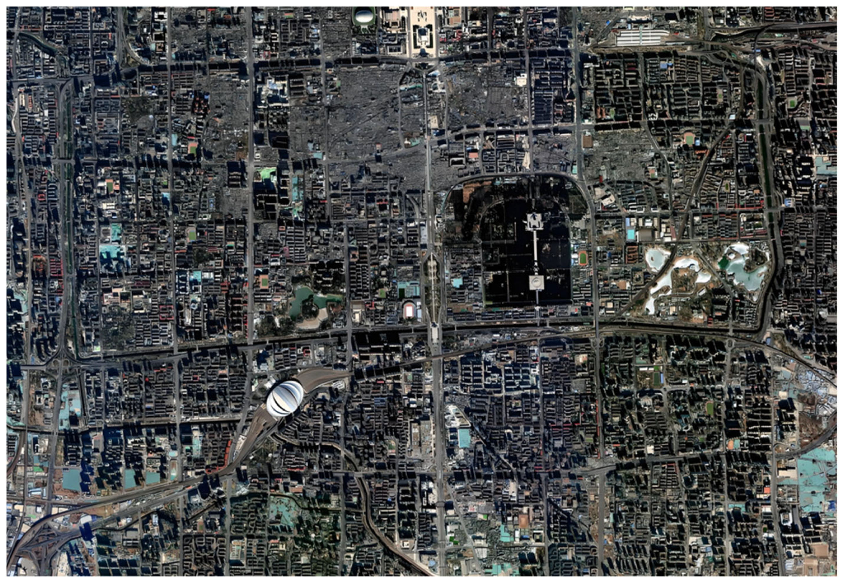
- High-resolution satellite remote sensing image technology is employed to acquire urban geographic information data. A communication link model for the urban environment is established based on an accurate city model, incorporating influencing factors such as building occlusion and diffraction loss.
- (2)
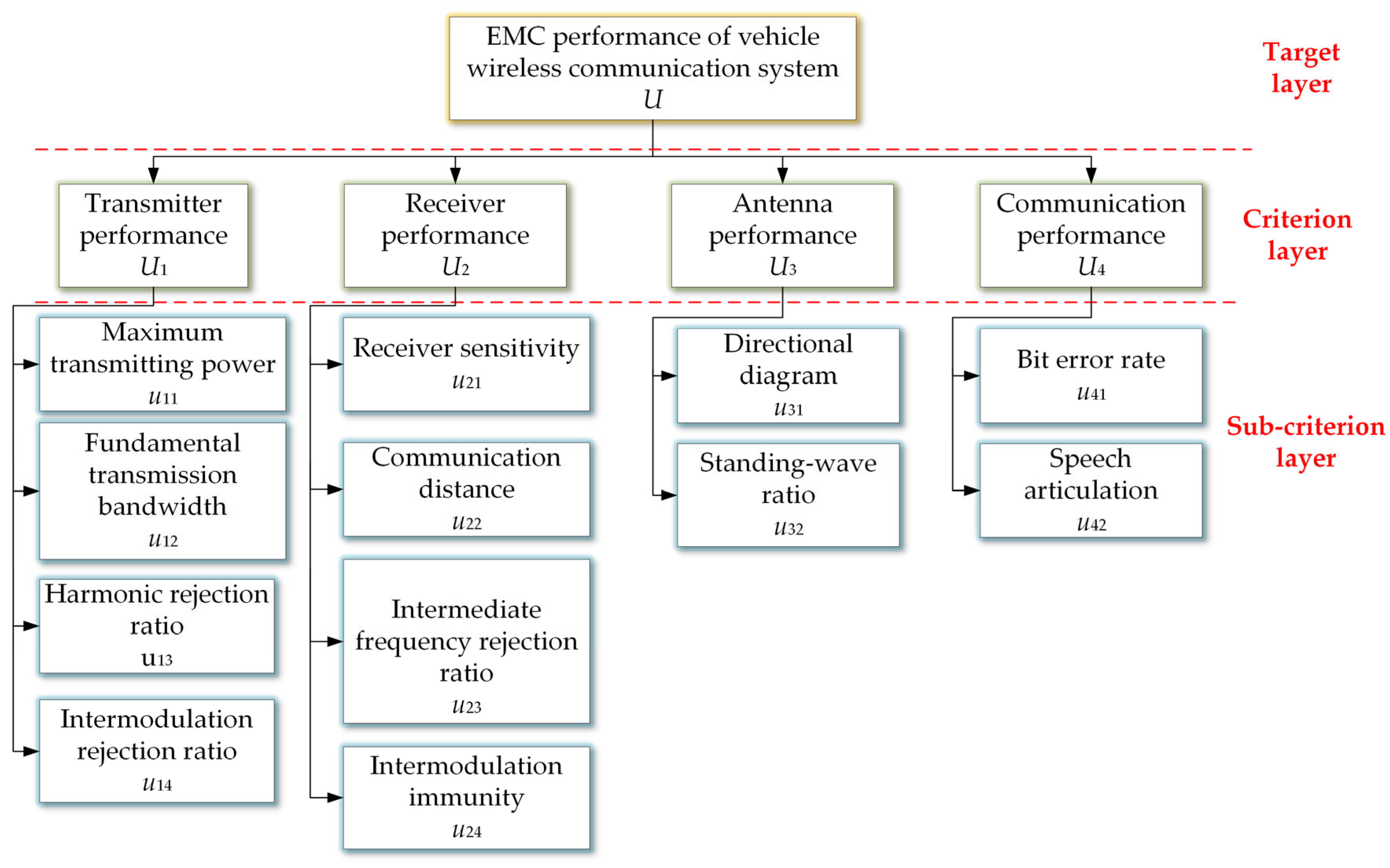
- Addressing the communication requirements of vehicles in urban environments, key EMC performance indicators for the communication system are selected from three dimensions: communication quality, anti-interference capability, and transmission reliability. A hierarchical structure model for EMC evaluation of vehicular wireless communication systems is developed, comprising the target layer, criterion layer, and sub-criterion layer.
- (3)
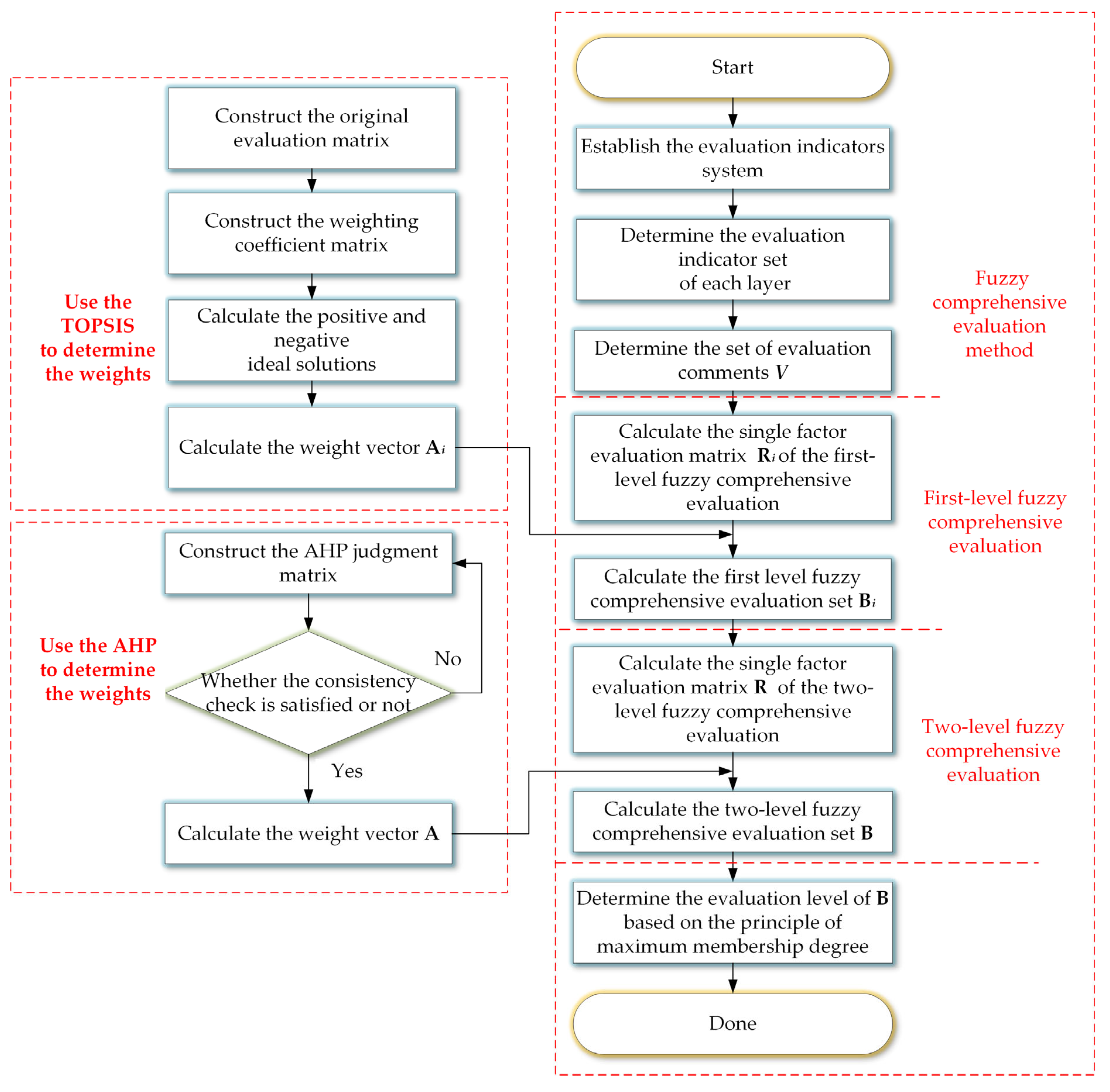
- The weights for the criterion layer and sub-criterion layer are determined using the quantitative technique for order preference by similarity to ideal solution (TOPSIS) method and the qualitative analytical hierarchy process (AHP) method, respectively. A comprehensive evaluation of the EMC of vehicular wireless communication systems is conducted through fuzzy comprehensive evaluation (FCE).
- (4)
- The communication model developed using high-precision satellite remote sensing images was employed to compare the average relative errors of BER (Bit Error Rate) and SNR (Signal-to-Noise Ratio) between simulated and measured results, thereby analyzing the system’s communication performance. Based on the evaluation results, the EMC performance of vehicular wireless communication systems in urban environments are analyzed. Leveraging high-resolution satellite image data, this analysis provides critical references for optimizing vehicular communication system design.
2. Related Evaluation Methods
2.1. AHP Method
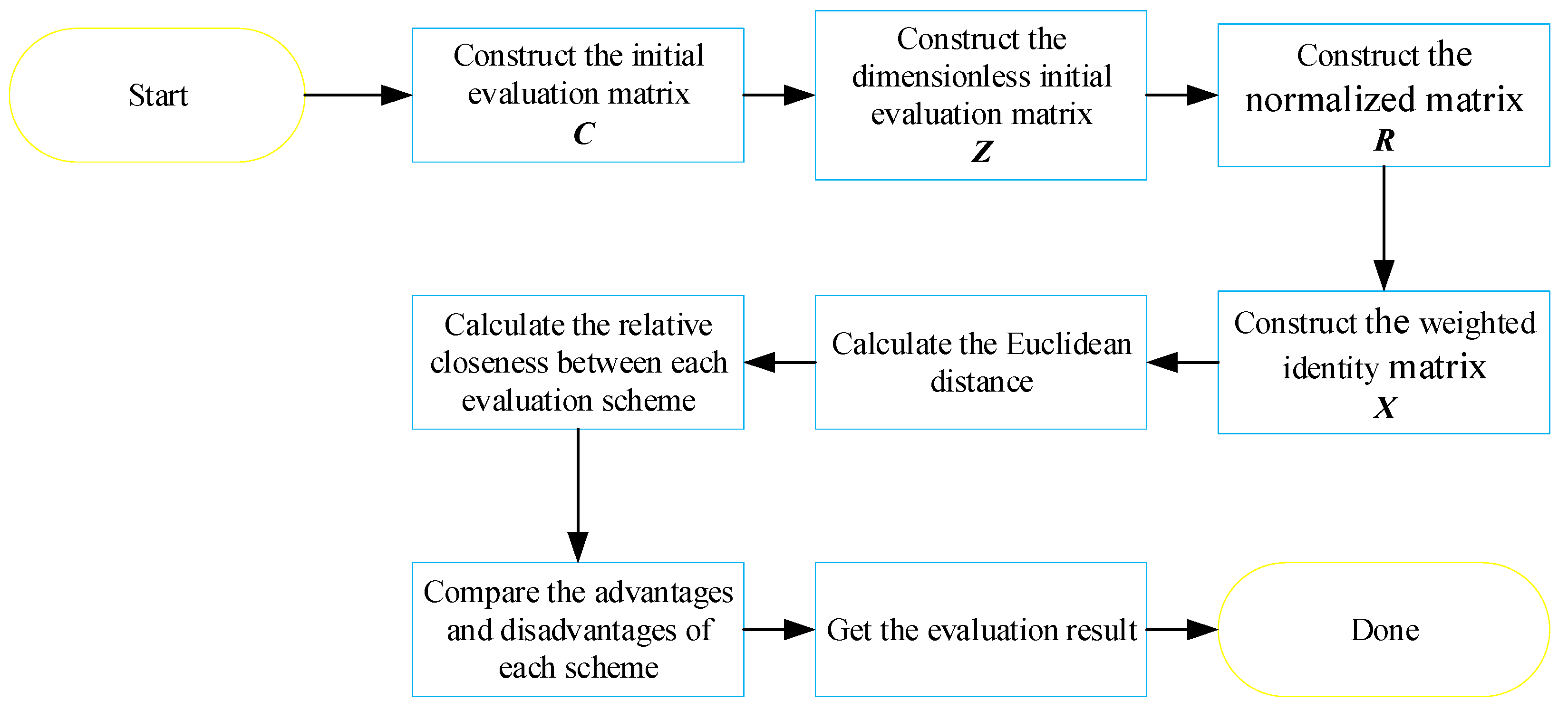
2.2. TOPSIS Method
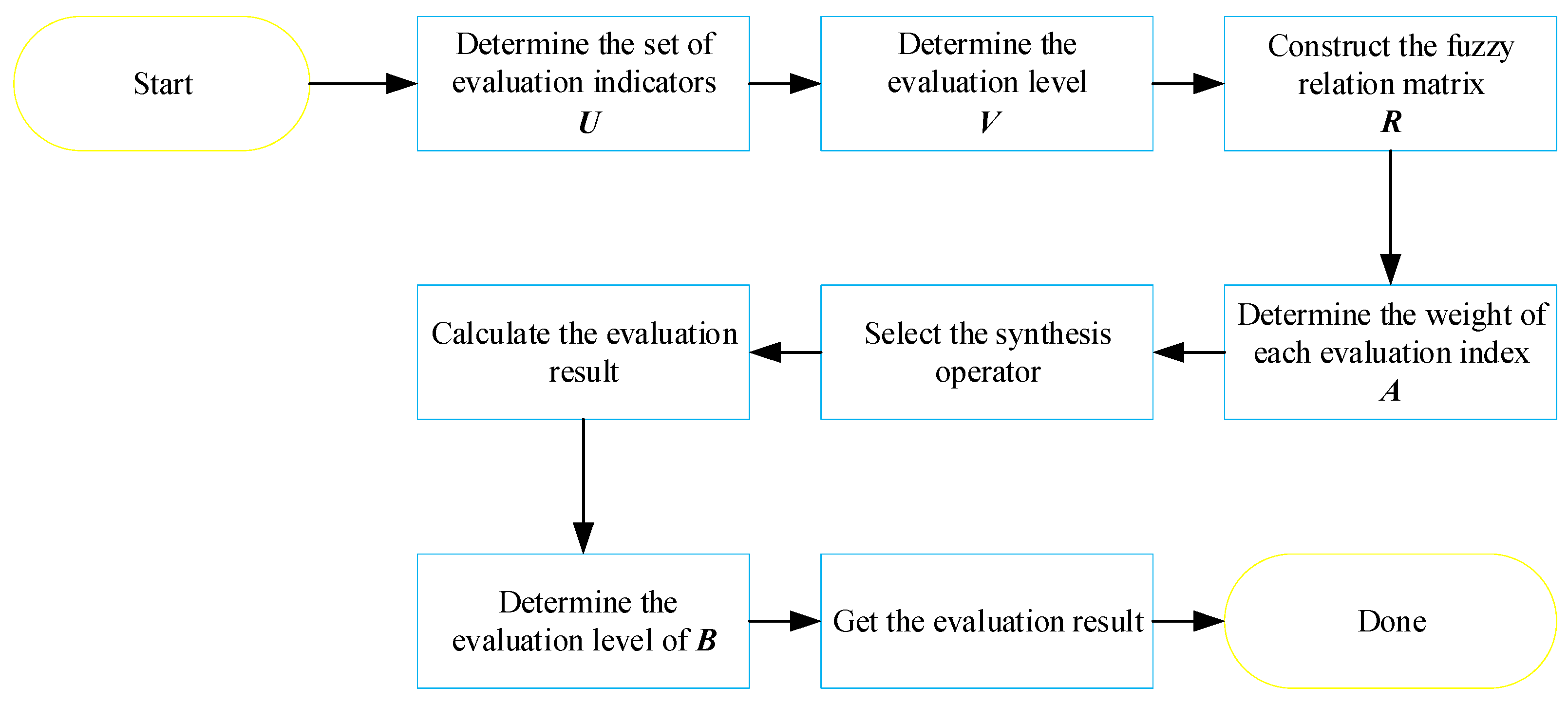
2.3. FCE Method
3. The Proposed Evaluation Method
3.1. Establish Indicators System
3.2. Key Techniques
3.3. Preprocessing Evaluation Data
3.3.1. Quantitative Indicators
3.3.2. Qualitative Indicators
3.4. Weights Determination
3.4.1. Weight Determination of the Sub-Criterion Layer (TOPSIS)
3.4.2. Weight Determination of the Criterion Layer (AHP)
3.5. Fuzzy Comprehensive Evaluation
3.5.1. First-Level FCE
3.5.2. Two-Level FCE
4. Experimental Validation and Analysis
4.1. Experimental Validation
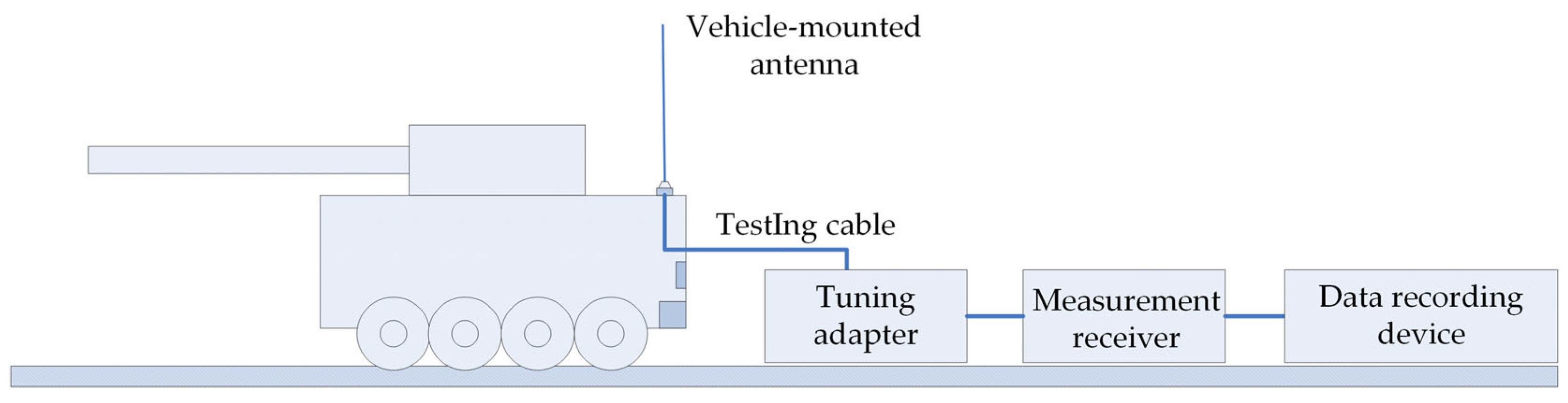
4.1.1. Experimental Setup
- (1)
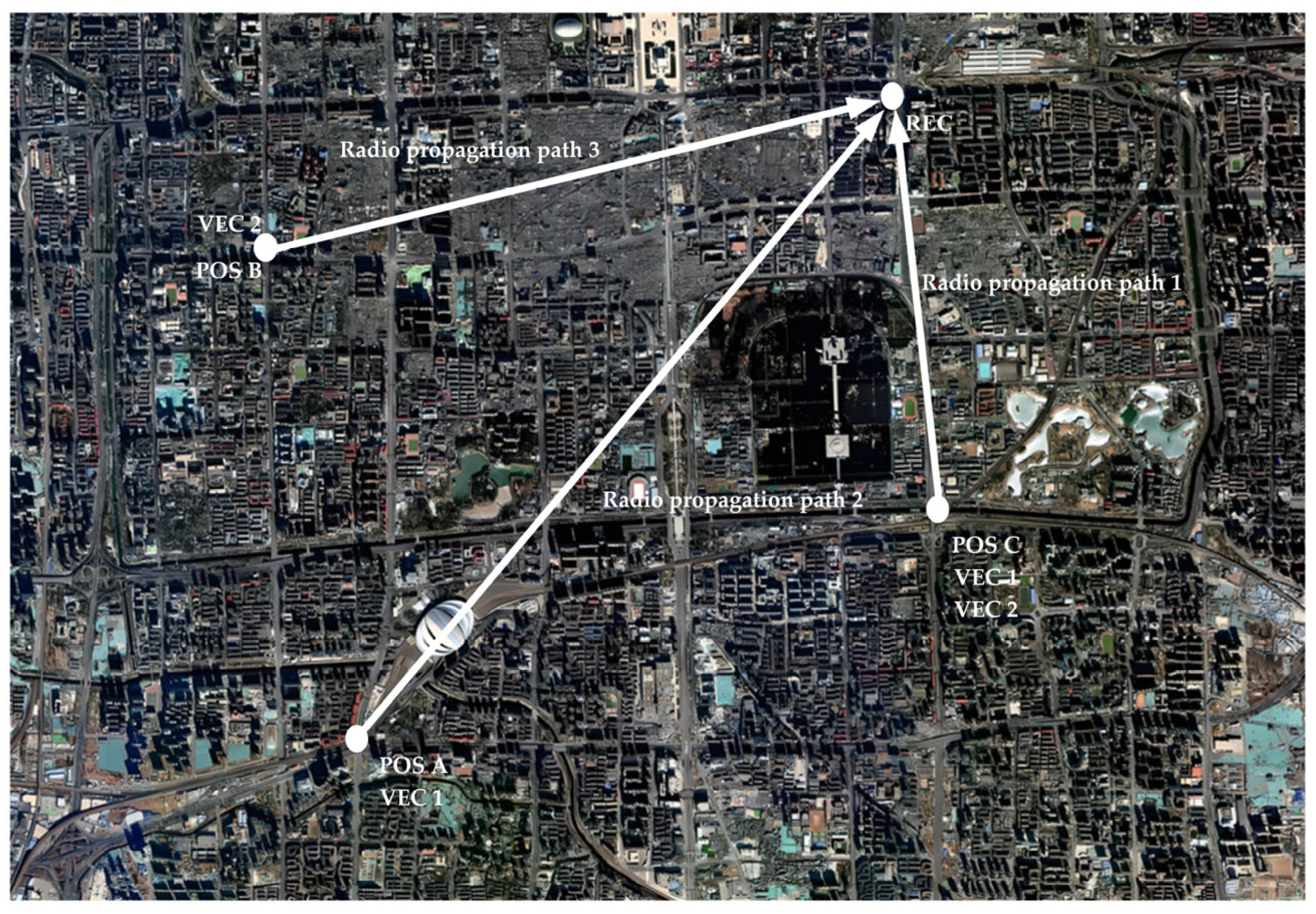
- Propagation distance: Direct correlation with path loss;
- (2)
- Obstruction characteristics: Including building density, dimensional parameters, and spatial distribution along the propagation path.
- (1)
- Same-position, same-vehicle control group: V1-PA-1 and V1-PA-2.
- (2)
- Different-position, same-vehicle control group: V2-PB and V2-PC.
- (3)
- Same-position, different-vehicle control group: V1-PC and V2-PC.
- (4)
- Different-position, different-vehicle control group: V1-PC and V2-PB; V1-PA-1 and V2-PC (and other possible combinations).
4.1.2. TOPSIS Method Determines the Weights of the Criterion Layer
4.1.3. AHP Determines the Weights of the Criterion Layer
4.1.4. Comprehensive Evaluation
4.2. Discussion and Analysis
4.2.1. Sensitivity Analysis of Weights Change
- (1)
- Only the TOPSIS method was employed for weight calculation.
- (2)
- Only the AHP method was employed for weight calculation.
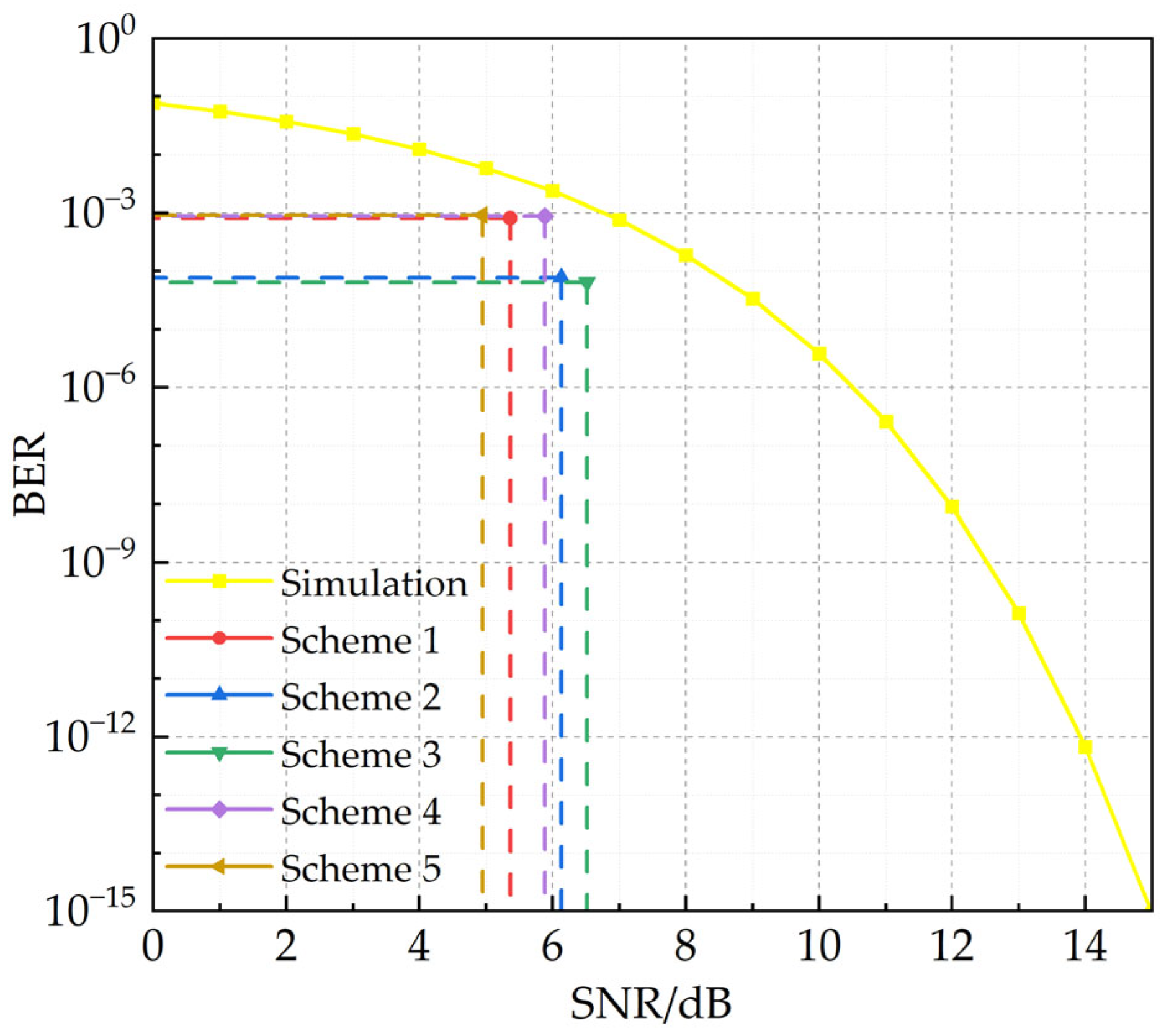
4.2.2. Communication Performance Analysis
4.2.3. EMC Analysis
- (1)
- All experimental schemes
- (2)
- Same-Position, Same-Vehicle control experiment group (V1-PA-1 vs. V1-PA-2)
- (3)
- Different-Position, Same-Vehicle control experiment group (V2-PC vs. V2-PB)
- (4)
- Same-Position, Different-Vehicle control experiment group (V1-PC vs. V2-PC)
- (5)
- Different-Position, Different-Vehicle control experiment group (V1-PC vs. V2-PB and V1-PA-1 vs. V2-PC)
5. Conclusions
Author Contributions
Funding
Institutional Review Board Statement
Informed Consent Statement
Data Availability Statement
Acknowledgments
Conflicts of Interest
References
- Aiello, O.; Crovetti, P. Characterization of the Susceptibility to EMI of a BMS IC for Electric Vehicles by Direct Power and Bulk Current Injection. IEEE Lett. Electromagn. Compat. Pract. Appl. 2021, 3, 101–107. [Google Scholar] [CrossRef]
- Wang, K.; Lu, H.; Chen, C.; Xiong, Y. Modeling of System-Level Conducted EMI of the High-Voltage Electric Drive System in Electric Vehicles. IEEE Trans. Electromagn. Compat. 2022, 64, 741–749. [Google Scholar] [CrossRef]
- Wang, K.; Lu, H.; Li, X. High-Frequency Modeling of the High-Voltage Electric Drive System for Conducted EMI Simulation in Electric Vehicles. IEEE Trans. Transp. Electrif. 2023, 9, 2808–2819. [Google Scholar] [CrossRef]
- Gajbhiye, P.; Achari, K.N.; Balakrishna, G.; Kumar, M.V. An Approach to Mitigate the EMI Noise Effect in Vehicle-to-Grid (V2G) System. In Proceedings of the 2021 2nd Global Conference for Advancement in Technology (GCAT), Bangalore, India, 1–3 October 2021; pp. 1–6. [Google Scholar]
- Qian, W.; Yang, Y.; Peng, J.; Cao, H.; Li, X.; Gao, Y.; Lei, J. EMI Modeling for Vehicle Body using Characteristic Mode Analysis. In Proceedings of the 2022 Asia-Pacific International Symposium on Electromagnetic Compatibility (APEMC), Beijing, China, 1–4 September 2022; pp. 732–734. [Google Scholar]
- Qian, W.; Yang, Y.; Peng, J.; Cao, H.; Li, X.; Gao, Y.; Lei, J. Vehicle electromagnetic interference suppression using characteristic mode analysis. In Proceedings of the 2022 Asia-Pacific International Symposium on Electromagnetic Compatibility (APEMC), Beijing, China, 1–4 September 2022; pp. 427–429. [Google Scholar]
- Mutoh, N.; Nakanishi, M.; Kanesaki, M.; Nakashima, J. EMI noise control methods suitable for electric vehicle drive systems. IEEE Trans. Electromagn. Compat. 2005, 47, 930–937. [Google Scholar] [CrossRef]
- Pliakostathis, K. Research on EMI from Modern Electric Vehicles and their Recharging Systems. In Proceedings of the 2020 International Symposium on Electromagnetic Compatibility-EMC EUROPE, Rome, Italy, 23–25 September 2020; pp. 1–6. [Google Scholar]
- Jiang, L.; Liu, H.; Zhang, X. Analysis on EMC influencing factors of electric vehicle wireless charging system. In Proceedings of the 2021 IEEE International Joint EMC/SI/PI and EMC Europe Symposium, Raleigh, NC, USA, 26 July–13 August 2021; pp. 285–290. [Google Scholar]
- Alcaras, A. EMC Performances of a Land Army Vehicle to Respect Integrated Radios Reception Sensitivity: Typical Perfor-mances Needed for “Fitted for Radio (FFR)” Land Vehicle. In Proceedings of the 2018 International Symposium on Electro-magnetic Compatibility (EMC EUROPE), Amsterdam, The Netherlands, 27–30 August 2018; pp. 303–308. [Google Scholar]
- Gkatsi, V.; Vogt-Ardatjew, R.; Leferink, F. Risk-based EMC System Analysis Platform of Automotive Environments. In Proceedings of the 2021 IEEE International Joint EMC/SI/PI and EMC Europe Symposium, Raleigh, NC, USA, 26 July–13 August 2021; pp. 749–754. [Google Scholar]
- Zhao, T.; Liu, X.; Sun, P.; An, M.; Mu, X. EMC Vehicle-Level Layout Design for Railway Vehicles in Complex Electromagnetic Environment. In Proceedings of the 2021 11th International Conference on Information Technology in Medicine and Education (ITME), Wuyishan, China, 19–21 November 2021; pp. 231–236. [Google Scholar]
- Hein, J.; Hippeli, J.; Eibert, T.F. Efficient EMC Parameter Analysis for the Verification of Complex Automotive Simulation Models by the Utilization of Design of Experiments. IEEE Trans. Electromagn. Compat. 2018, 60, 1965–1973. [Google Scholar] [CrossRef]
- Klotz, F.; Röbl, M.; Körber, B.; Müller, N. New standardized EMC evaluation methods for communication transceivers. In Proceedings of the2018 IEEE International Symposium on Electromagnetic Compatibility and 2018 IEEE Asia-Pacific Symposium on Electromagnetic Compatibility (EMC/APEMC), Singapore, 14–18 May 2018; pp. 139–144. [Google Scholar]
- Jiang, L.; Liu, H.; Wang, C. Summary of EMC Test Standards for Wireless Power Transfer Systems of Electric Vehicles. In Proceedings of the 2021 Asia-Pacific International Symposium on Electromagnetic Compatibility (APEMC), Nusa Dua-Bali, Indonesia, 27–30 September 2021; pp. 1–4. [Google Scholar]
- Mortazavi, S.; Schleicher, D.; Eremyan, D.; Gheonjian, A.; Jobava, R.; Sinai, A.; Gerfers, F. Investigation of Possible EMC Interferences between Multi-Gig Communication Link and RF Applications in Vehicle. In Proceedings of the 2019 International Symposium on Electromagnetic Compatibility-EMC EUROPE, Barcelona, Spain, 2–6 September 2019; pp. 1100–1105. [Google Scholar]
- Uehara, H.; Watanabe, K.; Sakai, R.; Ashida, S.; Tanaka, S.; Nagata, M. Evaluation of Electromagnetic Interference Between Electromagnetic Noise from an Autonomous Vehicle and GPS Signals. In Proceedings of the 2024 IEEE Joint International Symposium on Electromagnetic Compatibility, Signal & Power Integrity: EMC Japan/Asia-Pacific International Symposium on Electromagnetic Compatibility (EMC Japan/APEMC Okinawa), Ginowan, Japan, 20–24 May 2024; pp. 426–428. [Google Scholar]
- Li, J.; Lei, J.; Chen, R.; Peng, Y.; Mao, S.; Zhang, B. Advances in the ICVEMCTest Standardization in, China-SAE. In Proceedings of the 2022 16th European Conference on Antennas and Propagation (EuCAP), Madrid, Spain, 27 March–1 April 2022; pp. 1–5. [Google Scholar]
- Wang, Y.M.; Xu, W.T. An improved multi-level weighting additive summation method for electromagnetic compatibility evaluation. In Proceedings of the 2018 IEEE International Symposium on Electromagnetic Compatibility and 2018 IEEE Asia-Pacific Symposium on Electromagnetic Compatibility (EMC/APEMC), Singapore, 14–18 May 2018; pp. 476–480. [Google Scholar]
- Cai, Q.M.; Deng, Q.; Cao, X.; Zhou, L.; Li, H.; Du, Z.Y.; Li, Y.; Zhu, Y.; Fan, J. EMC Evaluation of High-power Electronic System Based on Improved AHP-TOPSIS. In Proceedings of the 2024 Photonics & Electromagnetics Research Symposium (PIERS), Chengdu, China, 21–25 April 2024; pp. 1–6. [Google Scholar]
- Wang, Y.; Li, Y.; Zhang, S. Automatic Detection of War-Destroyed Buildings from High-Resolution Remote Sensing Images. Remote Sens. 2025, 17, 509. [Google Scholar] [CrossRef]
- Huang, D.H.; Wu, S.H.; Wu, W.R.; Wang, P.H. Cooperative radio source positioning and power map reconstruction: A sparse Bayesian learning approach. IEEE Trans. Veh. Technol. 2015, 64, 2318–2332. [Google Scholar] [CrossRef]
- Yuan, B.; Sehra, S.S.; Chiu, B. Multi-Scale and Multi-Network Deep Feature Fusion for Discriminative Scene Classification of High-Resolution Remote Sensing Images. Remote Sens. 2024, 16, 3961. [Google Scholar] [CrossRef]
- Wang, J. Sparse Bayesian learning-based 3D radio environment map construction—Sampling optimization, scenario-dependent dictionary construction, and sparse recovery. IEEE Trans. Cognit. Commun. Netw. 2024, 10, 80–93. [Google Scholar] [CrossRef]
- Tan, Y.; Sun, K.; Wei, J.; Gao, S.; Cui, W.; Duan, Y.; Liu, J.; Zhou, W. STFNet: A Spatiotemporal Fusion Network for Forest Change Detection Using Multi-Source Satellite Images. Remote Sens. 2024, 16, 4736. [Google Scholar] [CrossRef]
- Gu, X.; Yu, S.; Huang, F.; Ren, S.; Fan, C. Consistency Self-Training Semi-Supervised Method for Road Extraction from Remote Sensing Images. Remote Sens. 2024, 16, 3945. [Google Scholar] [CrossRef]
- Wang, J.; Zhu, Q.; Lin, Z.; Chen, J.; Ding, G.; Wu, Q.; Gu, G.; Gao, Q. Sparse Bayesian Learning-Based Hierarchical Construction for 3D Radio Environment Maps Incorporating Channel Shadowing. IEEE Trans. Wirel. Commun. 2024, 23, 14560–14574. [Google Scholar] [CrossRef]
- Gao, R.; Xu, X.; Chen, L.; Sun, Y.; Li, M.; Hou, C. Research on Risk Assessment Method for Power Grid Data Security Based on AHP. In Proceedings of the 2025 IEEE 8th Information Technology and Mechatronics Engineering Conference (ITOEC), Chongqing, China, 14–16 March 2025; pp. 799–803. [Google Scholar]
- Wu, Z.; Bai, B.; Guan, J.; Yu, Y. Risk Exploration Based on LSMT Model and AHP Fuzzy Comprehensive Evaluation Model. In Proceedings of the 2025 IEEE International Conference on Electronics, Energy Systems and Power Engineering (EESPE), Shenyang, China, 17–19 March 2025; pp. 1111–1117. [Google Scholar]
- Li, B.; Zhang, X.; Wang, B.; Yang, C.; Guo, Y.; Xiao, S.; Wei, W.; Wu, G. Multicriteria Decision-Making Model for Assessing the Aging Condition of Composite Insulators Using AHP-Entroped TOPSIS. IEEE Trans. Instrum. Meas. 2025, 74, 3515115. [Google Scholar] [CrossRef]
- Wang, K. Optimized Captain Selection Using Diffusion-Based Player Behavior Synthesis and Multicriteria Decision Making With Intuitionistic Rough Fuzzy Under Dombi-AHP and PROMETHEE Methods. IEEE Access 2025, 13, 78471–78489. [Google Scholar] [CrossRef]
- Yu, J.; Wanitwattanakosol, J. The Overview of Chinese Electrical Vehicle Components Supply Routes Selection by using Entropy Weight-TOPSIS Method. In Proceedings of the 2025 Joint International Conference on Digital Arts, Media and Technology with ECTI Northern Section Conference on Electrical, Electronics, Computer and Telecommunications Engineering (ECTI DAMT & NCON), Nan, Thailand, 29 January–1 February 2025; pp. 197–202. [Google Scholar]
- Cubukcuoglu, B.; Uzun, B.; Gokcekus, H.; Albarwary, S.A.; Ozsahin, D.U. The Comparative Analysis of the Effectiveness of the Energy Resources Using Fuzzy PROMETHE-TOPSIS Method. In Proceedings of the 2025 IEEE 22nd International Multi-Conference on Systems, Signals & Devices (SSD), Monastir, Tunisia, 17–20 February 2025; pp. 191–197. [Google Scholar]
- Du, X.; Wu, D.; Gai, J. An Improved FMEA Method Combining Component Importance and Fuzzy TOPSIS. In Proceedings of the 2024 6th International Conference on System Reliability and Safety Engineering (SRSE), Hangzhou, China, 11–14 October 2024; pp. 264–271. [Google Scholar]
- Li, R.; Yan, Y. Target Selection for Shore Firepower Support Based on Entropy Weight and TOPSIS Method. In Proceedings of the 2024 10th International Symposium on System Security, Safety, and Reliability (ISSSR), Xiamen, China, 16–17 March 2024; pp. 397–400. [Google Scholar]
- Jun, L.; Jun, L.; Yuchen, Z. Research on Fuzzy Hierarchical Comprehensive Evaluation Method for Multi Person Decision Making Based on Grey Relational Clustering. In Proceedings of the 2025 IEEE International Conference on Electronics, Energy Systems and Power Engineering (EESPE), Shenyang, China, 17–19 March 2025; pp. 1128–1134. [Google Scholar]
- Qiao, Y.; Li, J.; Zhao, L.; Su, X. A New Fuzzy Comprehensive Evaluation Method with Triangular Distribution for Protection Characteristics of Circuit Breaker with Oil Dashpot. In Proceedings of the 2024 IEEE 7th Advanced Information Technology, Electronic and Automation Control Conference (IAEAC), Chongqing, China, 15–17 March 2024; pp. 146–150. [Google Scholar]
- Gao, X.; Xu, X.; Yang, R.; Wang, X.; Liang, J.; Wu, S.; Yao, Y. Research on Comprehensive Evaluation System of High Proportional New Energy Power System Based on Fuzzy Analytic Hierarchy Process. In Proceedings of the 2024 6th International Conference on Energy Systems and Electrical Power (ICESEP), Wuhan, China, 21–23 June 2024; pp. 653–658. [Google Scholar]
- Li, Y.; Chen, T.; Huang, J.; Gao, W. An Integrated Evaluation of Novel Energy Storage Performance Based on Multilevel Fuzzy Comprehensive Evaluation Method. In Proceedings of the 2024 China International Conference on Electricity Distribution (CICED), Hangzhou, China, 12–13 September 2024; pp. 94–99. [Google Scholar]
- Ma, Y.; Lin, Q.; Shi, D.; Li, X. Evaluation Method of Radar Combat Effectiveness Based on CG-Fuzzy Comprehensive Evaluation. In Proceedings of the 2024 4th International Conference on Machine Learning and Intelligent Systems Engineering (MLISE), Zhuhai, China, 28–30 June 2024; pp. 118–123. [Google Scholar]


| (a) | |||||||||||
| Evaluation indicators | Yes (existence or good) | No (inexistence or bad) | |||||||||
| Significance | 1 | 0 | |||||||||
| (b) | |||||||||||
| 0.1 | 0.2 | 0.3 | 0.4 | 0.5 | 0.6 | 0.7 | 0.8 | 0.9 | |||
| Five levels | Worst | – | Bad | – | General | – | Good | – | Best | ||
| Seven levels | Worst | Worse | Bad | – | General | – | Good | Better | Best | ||
| Nine levels | Worst | Worse | Bad | Worse than general | General | Better than general | Good | Better | Best | ||
| 1 | 2 | 3 | 4 | 5 | 6 | 7 | 8 | 9 | |
| RI | 0 | 0 | 0.58 | 0.9 | 1.12 | 1.24 | 1.32 | 1.41 | 1.45 |
| Communication Path | 1 | 2 | 3 |
|---|---|---|---|
| Length (km) | 21 | 45 | 36 |
| Normalized difference built-up index (NDBI) (Within the 50 m buffer zones on both sides of the communication path) | 0.43 | 0.86 | 0.65 |
| Morphological description | Patchy sparse distribution | Grid-like high-density Pattern | Clustered high-density aggregation |
| Building density (Within the 50 m buffer zones on both sides of the communication path) | 34% | 63% | 41% |
| Experimental Sets | V1-PA-1 | V1-PA-2 | V1-PC | V2-PC | V2-PB |
|---|---|---|---|---|---|
| scheme | 1 | 2 | 3 | 4 | 5 |
| The maximum transmitting power | 102 | 103 | 105 | 99 | 106 |
| The fundamental transmission bandwidth | 670 | 750 | 720 | 580 | 780 |
| The harmonic rejection ratio | 54 | 51 | 49 | 43 | 56 |
| The intermodulation rejection ratio | 47 | 53 | 58 | 49 | 57 |
| The EMC Performance of Vehicle Wireless Communication System | ||||
|---|---|---|---|---|
| 1 | 2 | 3 | 2 | |
| 1/2 | 1 | 1/3 | 1 | |
| 1/3 | 3 | 1 | 2 | |
| 1/2 | 1 | 1/2 | 1 |
| Grades | Best | Better | Good | Normal | Bad |
|---|---|---|---|---|---|
| Score | ≥0.9 | <0.3 |
| Comparative Experiment | V1-PA-1 | V1-PA-2 | V1-PC | V2-PC | V2-PB |
|---|---|---|---|---|---|
| Evaluation score | 0.258 | 0.528 | 0.60 | 0.193 | 0.049 |
| Class | bad | good | good | bad | bad |
| Comparative Experiment | V1-PA-1 | V1-PA-2 | V1-PC | V2-PC | V2-PB |
|---|---|---|---|---|---|
| BER | |||||
| SNR (dB) | 5.36 | 6.13 | 6.51 | 5.88 | 4.94 |
Disclaimer/Publisher’s Note: The statements, opinions and data contained in all publications are solely those of the individual author(s) and contributor(s) and not of MDPI and/or the editor(s). MDPI and/or the editor(s) disclaim responsibility for any injury to people or property resulting from any ideas, methods, instructions or products referred to in the content. |
© 2025 by the authors. Licensee MDPI, Basel, Switzerland. This article is an open access article distributed under the terms and conditions of the Creative Commons Attribution (CC BY) license (https://creativecommons.org/licenses/by/4.0/).
Share and Cite
Zhang, G.; Zhang, X.; Chen, P.; Zhang, S.; Wu, F.; Qin, Y.; Xu, Q.; Lu, H. Electromagnetic Compatibility Evaluation for Vehicular Communication Systems Based on Urban High-Resolution Satellite Remote Sensing Images. Sustainability 2025, 17, 6340. https://doi.org/10.3390/su17146340
Zhang G, Zhang X, Chen P, Zhang S, Wu F, Qin Y, Xu Q, Lu H. Electromagnetic Compatibility Evaluation for Vehicular Communication Systems Based on Urban High-Resolution Satellite Remote Sensing Images. Sustainability. 2025; 17(14):6340. https://doi.org/10.3390/su17146340
Chicago/Turabian StyleZhang, Guangshuo, Xiu Zhang, Peng Chen, Shiwei Zhang, Fulin Wu, Yangzhen Qin, Qi Xu, and Hongmin Lu. 2025. "Electromagnetic Compatibility Evaluation for Vehicular Communication Systems Based on Urban High-Resolution Satellite Remote Sensing Images" Sustainability 17, no. 14: 6340. https://doi.org/10.3390/su17146340
APA StyleZhang, G., Zhang, X., Chen, P., Zhang, S., Wu, F., Qin, Y., Xu, Q., & Lu, H. (2025). Electromagnetic Compatibility Evaluation for Vehicular Communication Systems Based on Urban High-Resolution Satellite Remote Sensing Images. Sustainability, 17(14), 6340. https://doi.org/10.3390/su17146340