Temporal Convolutional Network with Attention Mechanisms for Strong Wind Early Warning in High-Speed Railway Systems

Abstract

High-speed railway (HSR) is a key transport mode for achieving carbon reduction targets and promoting sustainable regional economic development due to its fast, efficient, and low-carbon nature. Accurate wind speed forecasting (WSF) is vital for HSR systems, as it provides future wind conditions that are critical for ensuring safe train operations. Numerous WSF schemes based on deep learning have been proposed. However, accurately forecasting strong wind events remains challenging due to the complex and dynamic nature of wind. In this study, we propose a novel hybrid network architecture, MHSETCN-LSTM, for forecasting strong wind. The MHSETCN-LSTM integrates temporal convolutional networks (TCNs) and long short-term memory networks (LSTMs) to capture both short-term fluctuations and long-term trends in wind behavior. The multi-head squeeze-and-excitation (MHSE) attention mechanism dynamically recalibrates the importance of different aspects of the input sequence, allowing the model to focus on critical time steps, particularly when abrupt wind events occur. In addition to wind speed, we introduce wind direction (WD) to characterize wind behavior due to its impact on the aerodynamic forces acting on trains. To maintain the periodicity of WD, we employ a triangular transform to predict the sine and cosine values of WD, improving the reliability of predictions. Massive experiments are conducted to evaluate the effectiveness of the proposed method based on real-world wind data collected from sensors along the Beijing–Baotou railway. Experimental results demonstrated that our model outperforms state-of-the-art solutions for WSF, achieving a mean-squared error (MSE) of 0.0393, a root-mean-squared error (RMSE) of 0.1982, and a coefficient of determination ($R^2$) of 99.59%. These experimental results validate the efficacy of our proposed model in enhancing the resilience and sustainability of railway infrastructure.Furthermore, the model can be utilized in other wind-sensitive sectors, such as highways, ports, and offshore wind operations. This will further promote the achievement of Sustainable Development Goal 9.

1. Introduction

The transport sector is the largest contributor to global greenhouse gas emissions, accounting for around one-quarter of total emissions worldwide [1]. This substantial carbon footprint highlights the urgent need to reduce emissions in transportation and shift towards sustainable mobility in order to achieve the sustainable development goals. Rail transport is widely regarded as the most energy-efficient and environmentally friendly mode of transportation in both passenger and freight transport [2]. According to a report from the International Energy Agency (IEA), the amount of carbon dioxide emitted passenger/kilometer by rail transport is only one-sixth and one-eighth of that emitted by air travel and road transport, respectively [3]. Additional, rail freight consumes only one-ninth to one-thirtieth of the energy tonne–kilometer compared to road transport [4]. The high-speed railway (HSR) further leverages these advantages by offering high speed, large passenger capacity, and low environmental impact [5]. However, the safe and reliable operation of HSR systems faces challenges from extreme weather events intensified by climate change. Strong winds pose a serious threat to the safety and stability of HSR systems [6]. For instance, the Beijing Railway Bureau reported that on 12 August 2018, strong winds damaged seven overhead wires on the Beijing–Shanghai high-speed railway, suspending 46 trains. Similar incidents have occurred in Japan, Switzerland, and Australia [7]. Moreover, unnecessary deceleration of trains increases energy consumption and indirect carbon emissions. These events highlight the urgent need to provide future wind statuses and decision support for HSR systems.

To ensure safe and efficient operations under extreme wind environments, the Railway Bureau has equipped a strong-wind early-warning system (SWEWS) on most open railway lines. Specifically, wind sensors are installed approximately every 10 km along the railway line to collect real-time wind data and transfer them to a central server [6]. The predictive model uses the monitored wind information to forecast future wind speed (WS). When the predicted WS exceeds a predefined safety threshold, typically 15 m/s, the dispatcher makes proactive decisions in advance to slow down or stop trains [8]. The effectiveness of an SWEWS largely depends on how accurately and reliably it can predict future WSs.

Wind speed forecasting (WSF) is a type of time series forecasting (TSF) that has gained significant attention during past decades. Traditional WSF approaches include physical and statistical models. Physical models rely on multiple geographic and meteorological information to make predictions [9]. However, due to the complex environment alongside the railway line, the development of physical models for HSR would be inefficient and laborious. Statistical models can forecast outcomes based solely on historical WS data, but they typically require the input series to be linear and stable [10]. However, due to the sudden and random nature of strong wind events, WS sequences are usually nonlinear and unstable. Thus, statistical models are not suitable for WSF.

Deep neural networks (DNNs) have stronger nonlinear fitting capabilities [11]. In the last decade, with the rapid development of deep learning (DL) technology, DNN-based models have achieved great success in electricity load forecasting [12,13,14], traffic forecasting [15,16,17], WS interval forecasting [18,19,20], and other TSF tasks. These successes have accelerated the advancement of DNN-based WSF. Recurrent neural networks (RNNs) represented by long short-term memory (LSTMs) [21] and gated recurrent units (GRUs) [22], with their unique recurrent structure, excel at capturing long-term dependencies in WS sequences, making them well suited for TSF tasks [23]. Convolutional neural networks (CNNs), another important branch of DNNs, can capture local temporal patterns [24]. However, their ability to model long-term dependencies is limited. To address this, researchers often combine CNNs and RNNs, leveraging their respective strengths in capturing long-term trends and short-term fluctuations [25,26]. For example, Shen et al. [27] proposed a CNN-LSTM model for multi-step WSF. The experimental results demonstrated that the hybrid network has better forecasting performance than the single network.

However, these hybrid network-based models have several limitations when applied to the HSR system. (1) These methods may lose important temporal information when processing long sequences [6]. (2) They often assume that the variation in time series is monotonic, meaning that the WS data at each time step have a cumulatively increasing effect on the model. In a real railway environment, WS variations are often abrupt and uncertain due to the influence of dynamic environmental factors (e.g., sudden storms and strong short-term convection activities) [28]. These transient WS changes do not follow a monotonic pattern and often occur unexpectedly, making it challenging for these models to accurately capture these sudden changes. (3) The convolution operation of CNN introduces future point-in-time data during training. However, the future wind data are unknown in real-world applications.

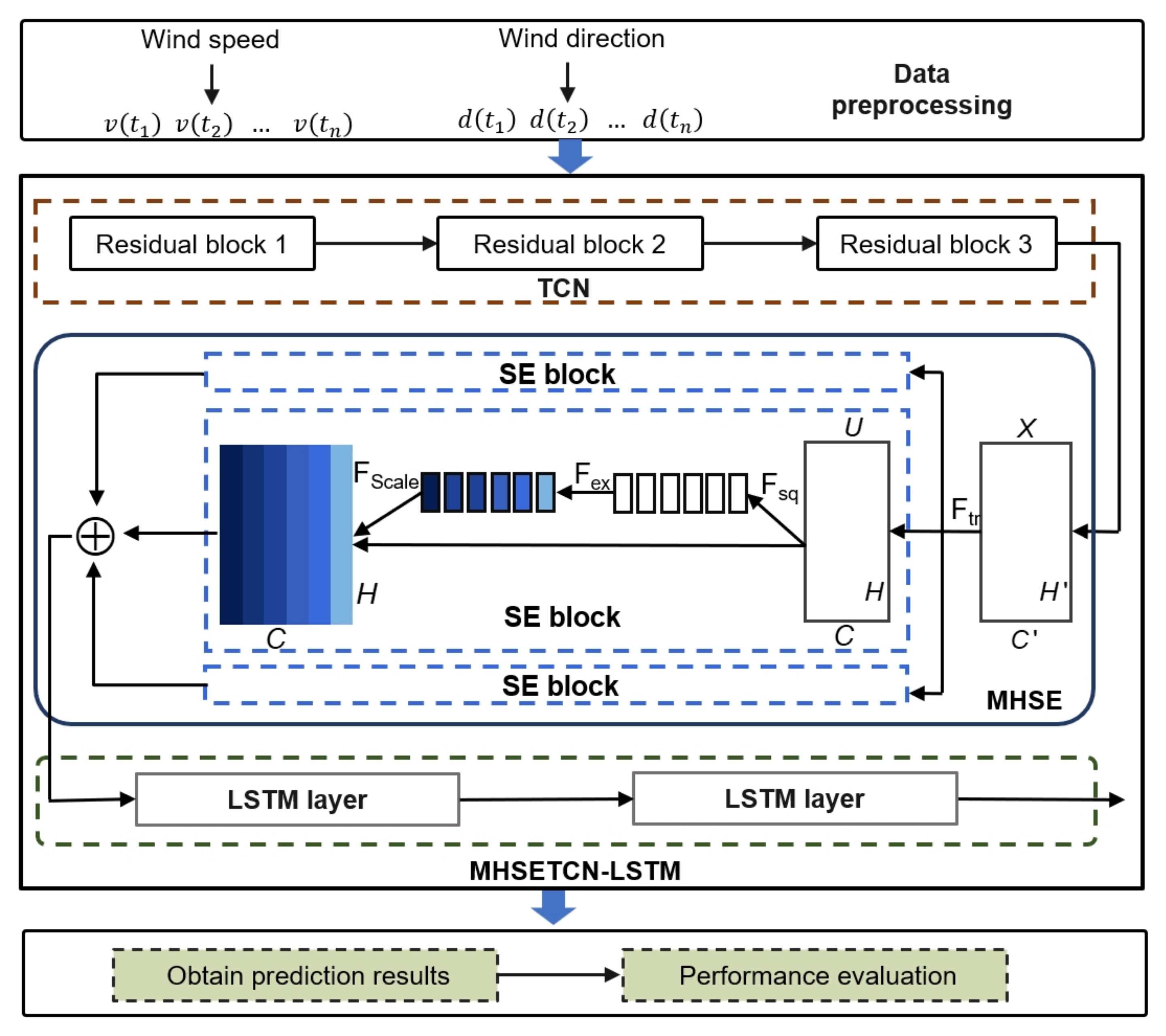
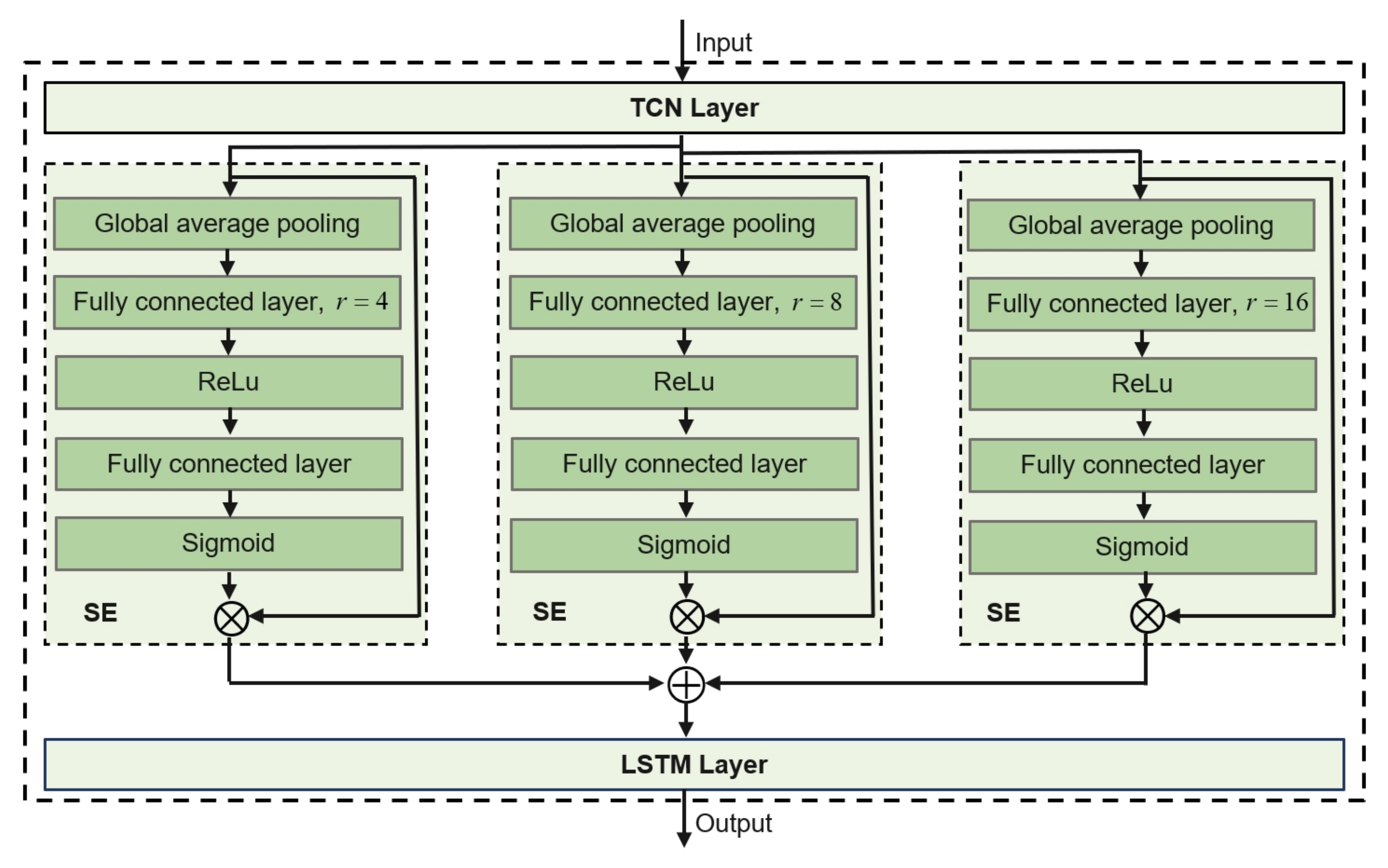
To address these issues, we propose a new hybrid model, MHSETCN-LSTM, which incorporates an attention mechanism to improve model performance in non-monotonic contexts. The squeeze-and-excitation (SE) mechanism allows the model to dynamically focus on the most relevant aspects of the input sequence at each time step by recalibrating the relationships between channels [29,30]. 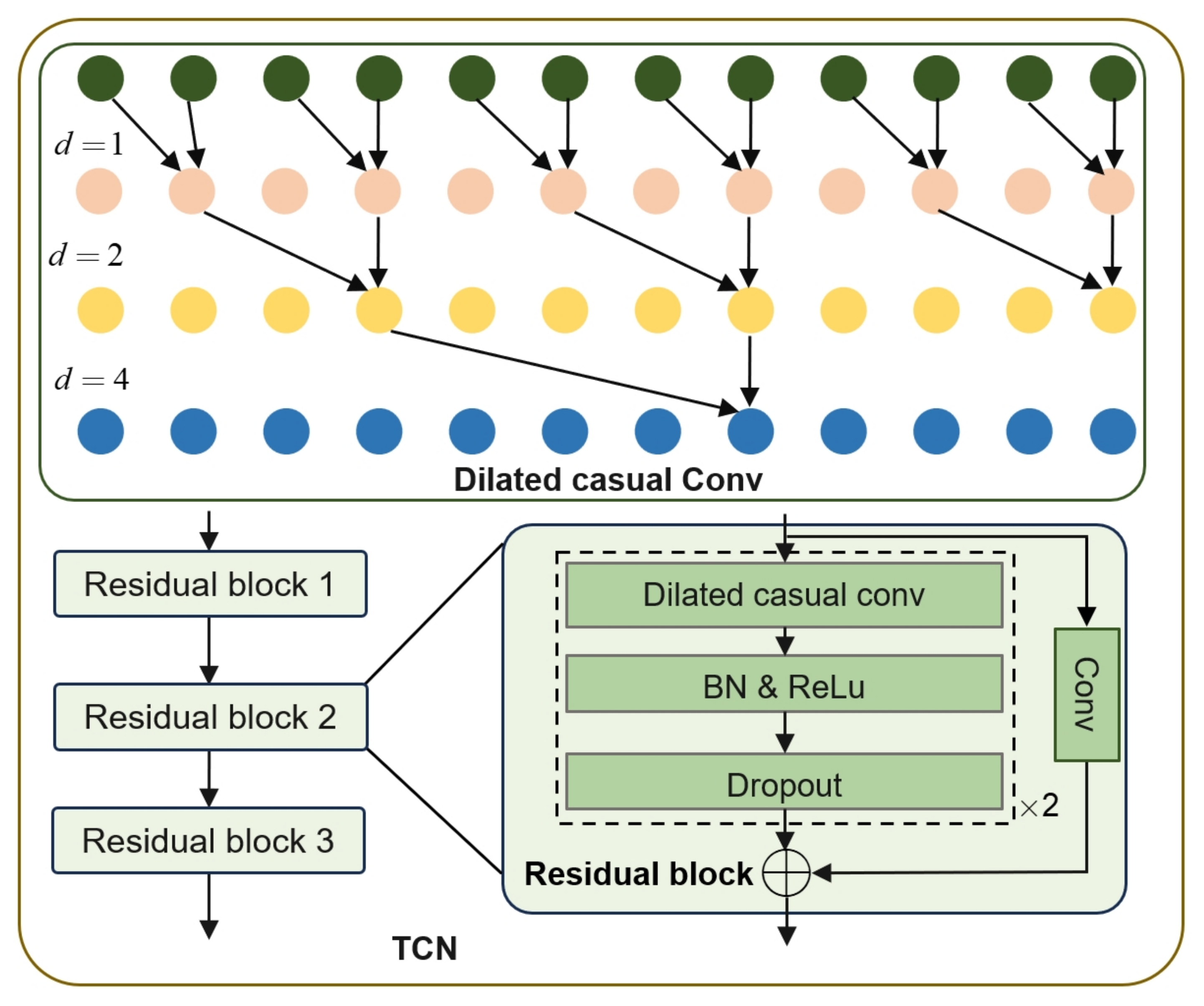The multi-head mechanism in the Transformer architecture enhances the model’s performance by capturing intrinsic patterns from multiple parallel subspaces [31,32,33]. Inspired by these outstanding works, we propose a novel attention mechanism, multi-head squeeze-and-excitation (MHSE), to adaptively focus on critical time steps from various perspectives. To avoid the convolution operation of CNNs introducing data from future time points during the training process, we employ a variant of CNNs, temporal convolutional networks (TCNs), to ensure that the prediction is merely based on current and past information. The customized CNN is then integrated with the LSTM unit to capture both short-term fluctuations and long-term trends, enabling better forecasting of wind behavior in complex environments.

Additionally, most existing strong-wind early-warning models focus merely on the WS, neglecting the important role of wind direction (WD) [34]. The angle between the WD and railway alignment affects the aerodynamic resistance and lateral force on trains [35]. For example, when the wind direction is between ${75}^{°}$ and ${95}^{°}$ relative to the railway alignment, strong cross-winds can greatly increase aerodynamic forces, potentially causing the train to overturn or even derail. Thus, incorporating WD into forecasting models is crucial for SWEWSs. The WD ranges from $0^{°}$ to ${360}^{°}$, forming a complete circle with clear periodicity. This periodic nature causes small numerical errors to be amplified. For instance, if a prediction error causes the WD to shift from ${359}^{°}$ to $1^{°}$, the numerical difference is large, but in reality, this change in WD is minimal. To address this, we apply a trigonometric transformation to the WD by predicting its sine and cosine values, preserving its periodicity and improving the reliability of the forecast. By incorporating WD as an additional feature, the proposed model MHSETCN-LSTM provides a more comprehensive understanding of the wind environment, further enhancing the accuracy and reliability of forecasting. The main contributions of this paper can be outlined as follows:

• We present a strong-wind early-warning framework that incorporates both wind speed and wind direction features, utilizing a hybrid network with an attention mechanism to enhance prediction accuracy for HSR systems.
• We propose a novel hybrid network, MHSETCN-LSTM, that integrates CNN, LSTM, and attention mechanisms to improve the accuracy and robustness of strong wind forecasting for high-speed rail systems. The attention mechanism enables adaptive focus on critical time steps, enhancing the model’s capability to detect and respond to abrupt and transient WS changes.
• We introduce wind direction as an additional feature to improve the model’s understanding of wind behavior, enhancing its capability to support HSR safety and operations.
• We conduct extensive experiments using real-world wind data collected from sensors along the Beijing–Baotou railway. The experimental results show that our method performs better than state-of-the-art approaches.

The rest of the paper is organized as follows. Section 2 briefly describes the related work on WSF and Section 3 details the proposed strong-wind early-warning framework. The comparison results and discussion are shown in Section 4. Section 5 summarizes the conclusion and discusses future work.

2. Related Works

Wind speed forecasting (WSF) plays a vital role in high-speed railway (HSR) systems [36]. Accurate predictions are essential to ensure the safe operation of trains. This section reviews relevant WSF studies. WSF is inherently challenging due to the nonlinear and nonstationary nature of wind [37]. Researchers have explored various approaches to improve prediction accuracy. These works can be divided into three categories: physical-based methods, statistical-based methods, and deep learning (DL)-based methods.

The physical-based methods utilize various physical parameters to predict WS. For instance, Zjavka et al. [38] modeled the relationships between meteorological features (i.e., pressures, temperature, etc.) and WSs to make predictions. However, the construction of a physical-based method requires heavy computation power support, which makes them impractical for complex railway environments.

On the other hand, statistical models like the Kalman filter [39], extreme learning machine (ELM) [40], autoregressive moving average model (ARMA) [41], and autoregressive integrated moving average (ARIMA) [42] are commonly used for linear TSF. While these methods can produce accurate forecasts for linear time series, they often struggle to capture nonlinear and dynamic patterns [9]. Thus, statistical-based methods are unsuitable for processing data that exhibit complicated nonlinear characteristics.

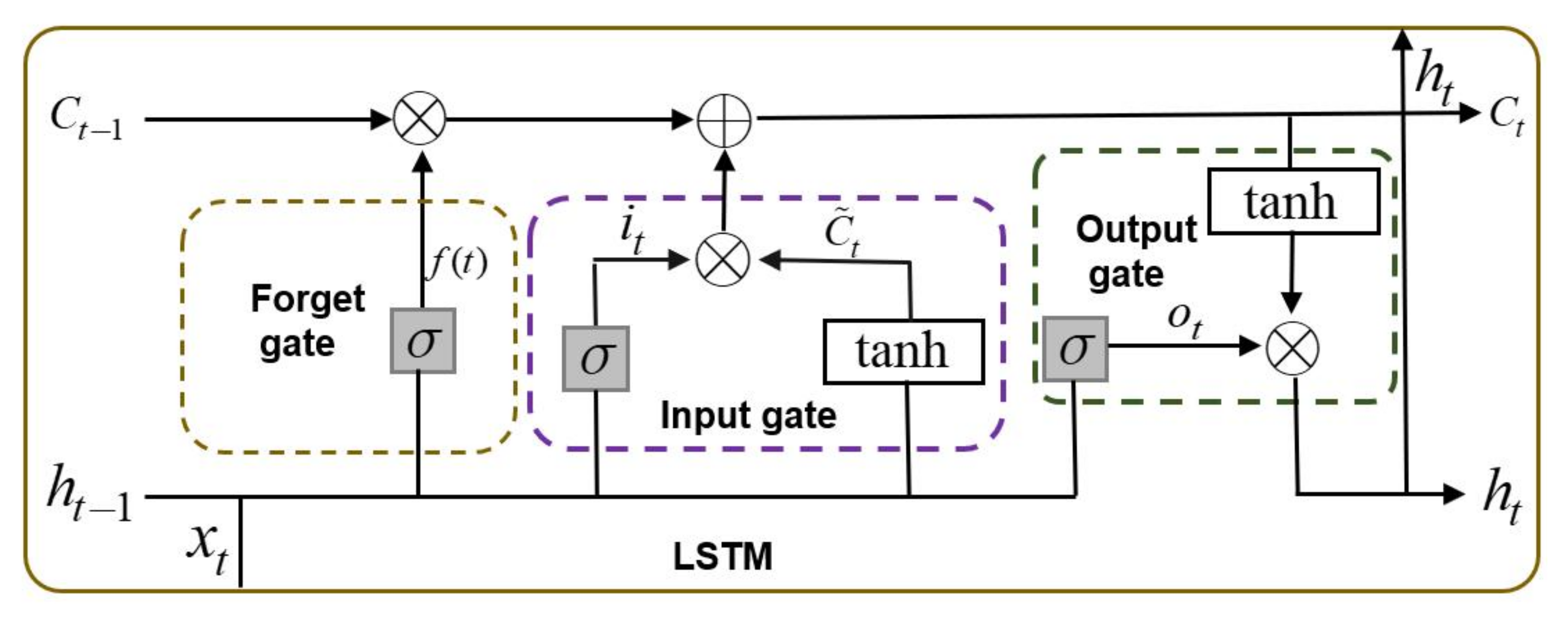
Recently, DL techniques have provided a new perspective to solve nonlinear TSF problems. Duan et al. [43] predicted future WSs by an RNN. Liu et al. [44] found that RNN is particularly effective in extracting the temporal dependence due to its unique structure. However, standard RNN architecture suffers from gradient vanishing, which limits their performance on long sequences [45]. LSTM addressed this problem by introducing three different gate structures to manage the retention, discarding, and transmission of information [26]. Convolutional neural networks (CNNs) excel at identifying short-term wind speed fluctuations (such as sudden gusts) based on their local receptive fields. The integration of CNN and RNN has gained considerable attention for harnessing their complementary strengths. For instance, Zhao et al. [25] employed a WSF model that combines CNN and GRU (a variant of RNN) to capture both long-term and short-term information in raw WS data [46]. Similarly, Zhu et al. [47] proposed a CNN-LSTM framework to simultaneously capture the temporal and spatial dependencies. Experiment results show that the prediction accuracy of the hybrid model is superior to that of a single model. In summary, while the physics-based WSF method relies on meteorological theory, its high computational resource requirements make it challenging to meet the real-time demands of railway applications. Statistical models can handle linear dynamics but struggle to capture the complex nonlinear patterns of wind. Deep learning methods, such as RNN and CNN, effectively overcome these limitations. Despite these advancements, current hybrid models have several limitations. Firstly, these methods inevitably lose several temporal correlations when dealing with long sequences. Second, they treat all time steps equally, which is suboptimal for WSF tasks. During extreme weather events, certain moments have a greater impact on prediction results. Thus, the prediction models need to dynamically adjust their focus to important key time steps. The attention mechanism can address this challenge by adaptively focusing on the most relevant parts of the input sequence at each time step. Inspired by the success of CNN and LSTM integration and the advantages of the attention mechanism, we propose a novel hybrid network, MHSETCN-LSTM. The CNN component effectively captures short-term wind speed fluctuations, while the LSTM component models long-term temporal dependencies. The attention mechanism further enhances the model’s performance by adaptively focusing on key time steps, particularly during extreme weather events, thereby preserving essential temporal correlations.

3. Methodology

In this section, we present an overview of the proposed strong-wind early-warning framework, and then explain the details of each component.

3.1. Problem Definition and Overall Framework Architecture

The main objective of our study is to develop a DNN model that can predict future wind speed (WS) and wind direction (WD) values at a future time point based on historical observations of these variables. The historical observations for WS and WD are denoted as $V=\{v\left(t_1\right),v\left(t_2\right),\dots ,v\left(t_n\right)\}$ and $D=\{d\left(t_1\right),d\left(t_2\right),\dots ,d\left(t_n\right)\}$, respectively. The $v\left(t\right)$ and $d\left(t\right)$ represent the WS and WD at time step t, respectively. The goal is to forecast the WS $\widehat{v}\left(t_{n+k}\right)$ and WD $\widehat{d}\left(t_{n+k}\right)$ values at a future time step $t_{n+k}$, where k refers to the forecast horizon. The prediction model is expressed as a function f, which uses historical data as input and outputs the predicted WS and WD at the future time step:

$$\left\{\begin{array}{c}\widehat{v}\left(t_{n+k}\right)=f_v(V,{\theta }_v)\hfill \\ \widehat{d}\left(t_{n+k}\right)=f_d(D,{\theta }_d)\hfill \end{array}\right.$$

(1)

where $\theta$ is the trainable parameter of the model.

As illustrated in Figure 1, our framework consists of three main components: data preprocessing, complex temporal dependence capture via the MHSETCN-LSTM model, and performance evaluation. In the first part, we employ wind speed (WS) and wind direction (WD) to characterize wind behavior. To handle the periodic nature of WD, we apply a trigonometric transformation. The second part interprets the core idea of our framework. In the MHSETCN-LSTM, the temporal convolutional network (TCN) is initially used to capture short-term correlations and rapid fluctuations in WS and WD. TCN captures local temporal patterns and short-range dependencies through dilated causal convolution. These convolutions allow the network to focus on relevant local patterns while ensuring that the predictions at each time step are made without violating causality. The MHSE module enhances the model’s ability to focus on relevant temporal features at multiple scales. It achieves this by introducing a multi-head attention mechanism that applies different reduction ratios within the SE blocks. These reduction ratios allow the model to dynamically adjust the importance of different time steps based on the scale of temporal dependencies. The attention mechanism in the MHSE component reweights the features extracted by the TCN, enhancing the model’s responsiveness to sudden or significant changes in the wind behavior (e.g., sudden gusts). This allows the model to better capture complex temporal dependencies and focus on the most relevant information across varying time scales. LSTM networks are especially effective for working with sequential data, where long-range dependencies are crucial for making accurate predictions. The LSTM processes the enriched features provided by the TCN and MHSE, learning how past information influences future wind behavior over extended periods of time. By combining TCN, MHSE, and LSTM, the model can handle multi-scale temporal dependencies effectively. The TCN captures local patterns, the MHSE adjusts feature importance at different temporal scales, and the LSTM learns long-term trends, making the model more adaptable and robust for tasks that require capturing both short-term fluctuations and long-term patterns. After training is finished, the model output is then evaluated for performance. The details of these components are introduced below.

3.2. Wind Direction for Trigonometric Transformation

WD is a periodic variable that ranges from $0^{°}$ to ${360}^{°}$. Due to the periodic nature of angles, directly using angular values as regression targets for calculating mean-squared error (MSE) may lead to significant inaccuracies in error calculation [48]. For example, if the actual value is $0^{°}$ and the predicted value is ${360}^{°}$, the MSE will reflect a large error despite the two values representing the same WD. To address this issue, we employ a trigonometric transformation to convert the WD from angular values to two continuous variables:

$$D_{sin}=sin({\displaystyle \frac{wd}{{180}^{°}}}\times \pi )$$

(2)

$$D_{cos}=cos({\displaystyle \frac{wd}{{180}^{°}}}\times \pi )$$

(3)

The final predicted WD values are obtained from the predicted sine (sin) values $D_{sin}$ and cosine (cos) values $D_{cos}$ through the inverse calculation. This approach ensures that the model can accurately handle the cyclic nature of WD, avoiding errors caused by angular discontinuities.

3.3. Short-Term Fluctuation Extraction Module

HSR often traverses a variety of complex terrains, including mountain ranges, plains, canyons, and cross-sea bridges [49]. These geographical features can affect the behavior of the wind in unpredictable ways, especially at special locations such as bridges, where the airflow is either blocked or accelerated. This can cause transient fluctuations in WS and WD. To ensure the safety of HSR operations, it is therefore necessary to effectively detect short-term changes in WS and WD.

Traditional forecasting methods rely on smoothing techniques to predict future wind conditions. However, these methods are inadequate in capturing rapid, high-frequency fluctuation patterns. To address these challenges, we employ temporal convolutional networks (TCNs) to extract short-term changes in WS and WD over short time intervals. TCNs are utilized in the model’s front-end due to their effectiveness in capturing short-term dependencies and local fluctuations in WS and WD. Figure 2 illustrates the stacked dilated structure enabling wide receptive fields. Unlike RNNs, TCNs use parallel dilation convolution, allowing the network to respond quickly to abrupt changes without requiring continuous state updates.

As illustrated in Figure 2, the input data are processed by a TCN, which consists of three residual blocks. TCNs, a variant of CNN, retain computational efficiency by parallel processing. Unlike standard convolution operations in CNN, which can introduce unknown future data and lead to prediction inaccuracies, we design dilated causal convolution to prevent information leakage and expand receptive fields. As shown in Figure 2, in a dilated causal convolution layer, when the dilation parameter $d=n$, every n-th input is sampled once.

$$F\left(s\right)=\sum _{i=0}^{k-1}f\left(i\right)·X_{s-d·i}$$

(4)

where k denotes the filter size, $X_{s-d·i}$ represents the input sequence, s refers to the elements of X, and d is the dilation factor.

In our TCN architecture, the first residual block employs a dilated causal convolution layer with a filter size of 3 and 16 filters, while the second block employs the same filter size but with 32 filters. The third block continues this trend with a filter size of 3 and 64 filters. After each dilated causal convolution layer, batch normalization (BN) layer and ReLU operations are applied. The use of BN improves the network’s convergence speed and alleviates gradient vanishing issues. The ReLU activation function further enhances the model’s ability to express nonlinear relationships, allowing the TCN to learn the complex patterns in wind data. Additionally, as shown in Figure 2, the residual connection is also introduced to the TCN to prevent information fading between multiple layers.

$$F{\left(X\right)}^{\prime }=X+F\left(X\right)$$

(5)

3.4. Dynamic Weight Adjustment Module

The instability and sudden changes in wind can make predictions more complex. Traditional static weighting methods do not suffice in handling the inherent abrupt and instability changes in wind conditions. To overcome this challenge, we implement a multi-head squeeze-and-excitation (MHSE) attention mechanism that dynamically adjusts the model’s focus on key time steps from various perspectives.

The MHSE is a lightweight and portable model, and its structure is illustrated in Figure 1. The MHSE mechanism enhances the model’s responsiveness to sudden wind events by dynamically adjusting feature weights. The core of this mechanism is based on multiple parallel squeeze-and-excitation (SE) mechanisms. Each SE block comprises two main parts: the squeeze and the excitation operations. The squeeze operation generates global statistical information using global average pooling, as described in (6). The squeeze operation retains global statistics information, resulting in the data dimension change from (B, T, C) to (B, C). B is the batch size, T is the time step, and c is the number of channels.

$$z_c=Fsq\left(xc\right)={\displaystyle \frac{1}{H}}\sum _{i=1}^{H}xc\left(i\right)$$

(6)

The excitation operation employs two fully connected layers and an activation function that adaptively learns the weighting coefficients based on the global statistics obtained from the squeeze operation. The excitation operation achieves downscaling and upscaling, resulting in the data dimension change from (B, C) to (B, 1, C).

$$s=Fex\left(Fsq\right(xc),W)=\sigma \left(g\right(z,W\left)\right)=\sigma \left(W2\delta \right(W1z\left)\right)$$

(7)

where $X=[x_1,x_2,\dots ,x_c]$, $x_c$ represents the feature of size H for the c-th input. $\sigma$ and $\delta$ are the Sigmoid and ReLU activation functions. $W1$ and $W2$ indicate the weights of the first and second fully connected layers, respectively.

Different individuals observe the same object with varying levels of attention [31]. By integrating information from multiple perspectives, we can obtain a more comprehensive representation of the data, thus enhancing model performance. The multi-head mechanism combines the outputs of several SE blocks in parallel [50], which helps capture potential inter-dependencies across different time steps. For each SE block, the generated weight vector $s^i(i=1,2,3)$ is multiplied with the raw input to obtain the reweighed values. The outputs from all SE blocks are concatenated to obtain the final output. The dimension of the final output is still (B, T, C). The weights of these heads are multiplied by each other, which is equivalent to superimposing multi-scale attention on the same channel.

$$X^{\prime }=Concat(s^{1}X,s^{2}X,s^{3}X)$$

(8)

The implementation details of the MHSE attention module are shown in Figure 3. The number of attention heads in MHSE is set to 3, which means that three parallel SE blocks are processing the output data from the TCN. The reduction ratios for these SE blocks are set to 4, 8, and 16, respectively. Each SE block contains a global average pooling layer, two fully connected layers, a ReLU activation layer, and a Sigmoid activation layer. For each SE block, the generated weight vector is multiplied element-wise with the raw input to obtain the reweighted values. The outputs from different SE blocks are then fused using an element-wise addition strategy. This fusion strategy enables the model’s capability to focus on different aspects of temporal dependency across multiple attention heads.

3.5. Long-Term Dependency Learning Module

While short-term fluctuations in wind speed (WS) and wind direction (WD) are critical for safety in railway applications, understanding long-term dependencies is also vital for accurate forecasting of wind conditions. Large-scale weather patterns such as low-pressure zones, cold fronts, and monsoon patterns have a significant impact on wind behavior over long periods. These long-term dependencies interact with short-term fluctuations to form a complex wind environment.

To model these long-term dependencies, we design a long-term dependence learning module based on LSTM. The LSTM is a variant of the recurrent neural network (RNN). The structure of LSTM is shown in Figure 4. It effectively solves the gradient problem of RNNs by introducing three unique gates (input gate, forgetting gate, and output gate) to retain, forget, and transmit information in time series data. The gate mechanisms in the LSTM control the selective retention and transmission of information through a series of weights and biases [20]. Combined with the TCN and MHSE components, LSTM further enhances the model’s forecasting capability and accuracy in complex wind environments.

$$i_t=\sigma (W_i·[h_{t-1},x_t]+b_i)$$

(9)

$$f_t=\sigma (W_f·[h_{t-1},x_t]+b_f)$$

(10)

$${\tilde{C}}_t=tanh\left(W_c·\left[h_{t-1},x_t\right]+b_c\right)$$

(11)

$$C_t=f_t·C_{t-1}+i_t·{\tilde{C}}_t$$

(12)

$$o_t=\sigma \left(W_o·\left[h_{t-1},x_t\right]+b_o\right)$$

(13)

$$h_t=o_t·tanh\left(C_t\right)$$

(14)

where $i_t$, $f_t$, and $o_t$ are input gates, forgetting gates, and output gates, respectively. ${\tilde{C}}_t$ and $C_t$ are temporary and current cell states, respectively. $h_t$ and $h_{t-1}$ refer to the hidden layer states at time t and $t-1$, respectively. $x_t$ denotes the input sequence at time t.

By using two LSTM layers, we can effectively capture the long-term temporal dependencies in the data. The data processed by the MHSE module are fed into the first LSTM layer. The output after processing by the first LSTM layer is (B, T, C). The second layer LSTM processing compresses the time dimension and preserves the hidden state at the last moment. Therefore, the output dimension is (B, C).

4. Experiment and Evaluation

In this section, we describe the details of our experiments and answer the following research questions:

RQ1: How does the proposed method perform compared to other state-of-the-art WSF models?

RQ2: What is the impact of different components in our proposed method?

RQ3: How does the number of attention heads in MHSE affect performance?

4.1. Settings

4.1.1. Dataset

To ensure the safe operation of trains, several wind sensors are installed along the railway tracks to provide real-time wind information. We conducted an analysis of the historical wind observations near the Guanting Reservoir Grant Bridge. When the airflow passes over the bridge, the wind on both sides is restricted or lifted, resulting in high-speed airflow and a sudden increase in wind speed (WS). The monitoring site’s predominant wind direction (WD) is from the south to south–southwest (SSW), while the railway alignment is northeast–southwest. This indicates that cross-winds are common in the area. Strong cross-winds can exert lateral forces on a moving train, impacting its lateral stability and aerodynamic lift. This poses a serious threat to train stability and increases the risk of derailment and overturning. Therefore, monitoring the wind field in the area is critical to ensure train safety.

Due to these factors, we conducted a strong wind warning study based on the site near the Guanting Reservoir Grant Bridge. We selected a total of 28 days of continuous historical WS and WD observations with 1 s sampling intervals from sensors deployed near the Guanting Reservoir Bridge. The sampling period spanned from 1 February 2021 to 28 February 2021. There were no missing values in the sampled dataset. The dataset was divided into a training set and a test set, which accounted for $60\%$ and $40\%$ of the total dataset, respectively. To prevent any future data from influencing the training stage, the first $60\%$ of the whole dataset was used for training and the remaining was used for testing. The training dataset corresponds to the data time range from 1 February 2021 00:00:00 to 17 February 2021 19:12:00. The test dataset covers the subsequent time period from 17 February 2021 19:12:01 to 28 February 2021 23:59:59. Before inputting the data into the predictive model, the data were normalized based on max–min normalization and was inverse-normalized after prediction.

The statistical results for WS are summarized in

Table 1. Statistical analysis of wind speed data.

Mean (m/s)	Max (m/s)	SD (m/s)	p-Value	Skewness	Kurtosis
5.73	23.00	3.75	0.00	0.77	−0.07

. It can be observed that the WS peak reached 23.00 m/s. This exceeds the maximum WS of 15 m/s allowed for safe train operation. The standard deviation (SD) of WS is 3.75 m/s. A higher SD indicates a higher risk of sudden gusts. To analyze the distribution of the wind speed data, we conducted the Kolmogorov–Smirnov test. As shown in Table 1, the p-value for WS is 0.00, indicating that the WS data do not follow a normal distribution. Additionally, positive skewness and negative kurtosis suggest that the WS sequence has a right-skewed distribution with a flatter peak and lighter tails. These analyses indicate that the WS series shows a non-Gaussian distribution, high volatility, and long-term dependence. These characteristics pose significant challenges for accurate WSF.

4.1.2. Evaluation Criteria

To evaluate the forecasting performance of the proposed model, we employed three common performance indices, including mean absolute error (MAE), root-mean-squared error (RMSE), and coefficient of determination ($R^2$). Details of these performance indexes are listed below.

$$MAE={\displaystyle \frac{1}{n}}\sum _{i=1}^n\left|{\widehat{y}}_i-y_i\right|$$

(15)

$$RMSE=\sqrt{{\displaystyle \frac{1}{n}}\sum _{i=1}^n{({\widehat{y}}_i-y_i)}^2}$$

(16)

$$R^2=1-{\displaystyle \frac{{\displaystyle \sum _{i=1}^n}{(y_i-{\widehat{y}}_i)}^2}{{\displaystyle \sum _{i=1}^n}{(y_i-\overline{y})}^2}}$$

(17)

where n refers to the number of data samples. $y_i$ and ${\widehat{y}}_i$ are the actual and predicted value at the time point i, respectively.

4.1.3. Baselines

To verify the efficiency of the MHSETCN-LSTM model, we compared it with several baseline models under the same dataset and training process. The contrast models include convolutional neural networks (CNNs), long short-term memory networks (LSTMs), temporal fusion transformers (TFTs) [51], convolutional neural network (CNN)–long short-term memory (LSTM)–attention mechanism (CNN-LSTM-AM) [52], and deep residual network (DRN) [53]. These benchmark algorithms are briefly described below.

CNN: The one-dimensional CNN is commonly used to extract local association patterns from time series data. The CNN architecture contains five layers, including two convolutional layers, two pooling layers, and a flattened layer.

LSTM: The LSTM is better at capturing long-term dependencies than RNNs because they mitigate the gradient vanishing problem and enhance the ability to memorize information over longer periods of time.

TFT [51]: The TFT is a novel attention-based network architecture. It uses recurrent layers to extract local information and employs interpretable self-attention layers to handle long-term dependencies.

CNN-LSTM-AM [52]: This model combines CNN, LSTM, and attention mechanism for wind speed forecasting. CNN and LSTM are applied to extract spatial and temporal features from the wind sequences, respectively. The attention mechanism is introduced to enhance the ability to capture dynamics temporal patterns.

DRN [53]: Deep residual network (DRN) combines CNN and squeeze-and-excitation (SE) attention. The CNN is employed to extract temporal features from the wind data. The SE is used to recalibrate feature responses from convolutional layers.

4.2. Comparison with Existing Methods

In this section, we compare the performance of the MHSETCN-LSTM model with several state-of-the-art baseline models. The results are presented in

Table 2. Prediction error metrics of different methods for WSF (bold indicates the best, italics indicates the second-best).

Model	MSE	RMSE	${\mathit{R}}^2(\%)$
CNN	4.5132	2.1244	52.87
LSTM	2.9753	1.7249	68.93
DRN	0.6013	0.7754	93.72
CNN-LSTM-AM	0.0492	0.2219	99.49
TFT	0.6055	0.7781	88.70
MHSETCN-LSTM	0.0393	0.1982	99.59

. The MHSETCN-LSTM model demonstrates superior performance in comparison to all other baseline models across all performance metrics. Specifically, it achieves the lowest mean-squared error (MSE) of 0.0393, a root-mean-squared error (RMSE) of 0.1982, and the highest $R^2$ value of 99.59%.

The LSTM model excels in modeling long-term temporal dependencies and outperforms the CNN model in all evaluation metrics. However, it still exhibits suboptimal performance compared to hybrid models, such as DRN and CNN-LSTM-AM. One of the key limitations of the LSTM model is its inability to capture short-term fluctuations, which negatively impacts its overall predictive accuracy. DRN outperforms basic CNN and LSTM models, especially in handling deep feature extraction. However, DRNs lack the effective capture of long-period temporal dependencies, which is the strength of MHSETCN-LSTM prediction accuracy. The CNN-LSTM-AM achieves the second-highest $R^2$ of 99.49%. This result indicates that the CNN-LSTM-AM model is effective in capturing temporal dependencies. In CNN-LSTM-AM, the attention mechanism enables the model to focus on the important time step information in the sequence. However, despite its excellent performance, the CNN-LSTM-AM model is still inferior to our proposed model MHSETCN-LSTM. This is due to our proposed model using a novel attention mechanism to capture the complex dynamics in the wind data. The TFT is a novel attention-based network architecture for multi-horizon time series forecasting tasks. However, our prediction task only focuses on the value at the next time point. The complexity of TFT may increase the risk of overfitting, especially when data are limited or noisy, which is often the case in wind sensor records.

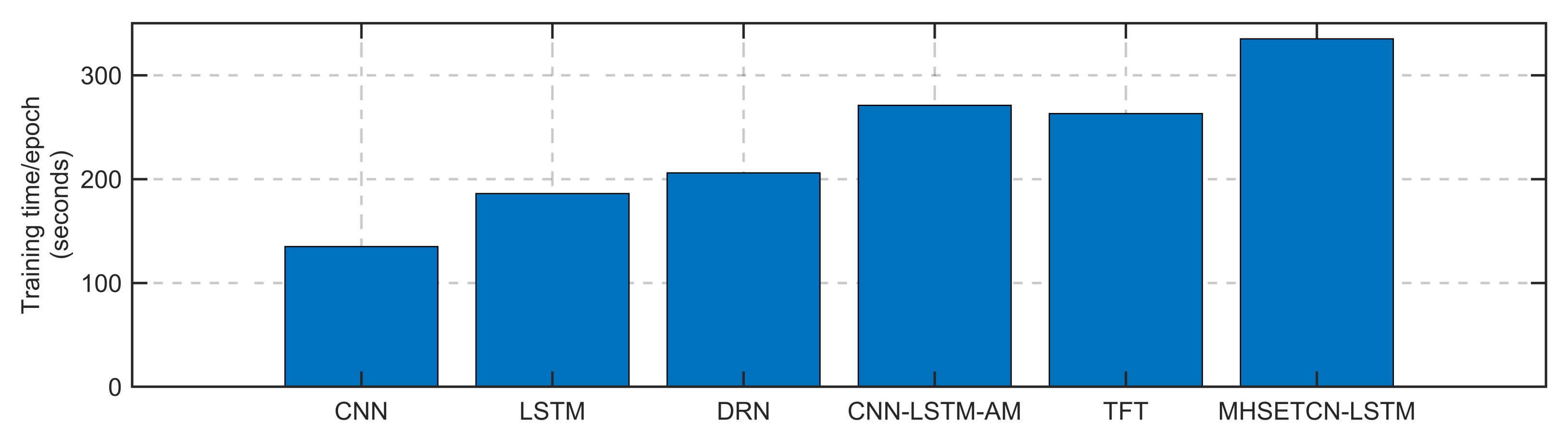
As shown in Figure 5, the computational cost of our proposed model during training is relatively high, taking about 335 s per epoch. This is slightly more than the 135 s required for CNN, 186 s for LSTM, 206 s for TCN, 271 s for DRN, and 263 s for TFT. However, the significant improvement in prediction accuracy makes this increased cost justifiable. The enhanced performance has resulted in more reliable and timely wind warnings, which in turn reduces unnecessary energy consumption, emergency braking, and service disruptions.

4.3. Performance Evaluation

According to the Code for Design of High-Speed Railway, a wind speed of 15 m/s is established as the operational safety threshold for speed restrictions. Specifically, trains of the CR400 series must reduce their speed when wind conditions exceed this limit, in line with national safety standards for train operations during adverse weather. Therefore, we consider 15 m/s as the classification boundary for strong wind events in this study, ensuring our evaluation aligns with real-world operational requirements.

Table 3. The confusion matrix for the MHSETCN-LSTM model.

	Predicted WS (Label 1)	Predicted WS (Label 0)
Real WS (label 1)	1749	1269
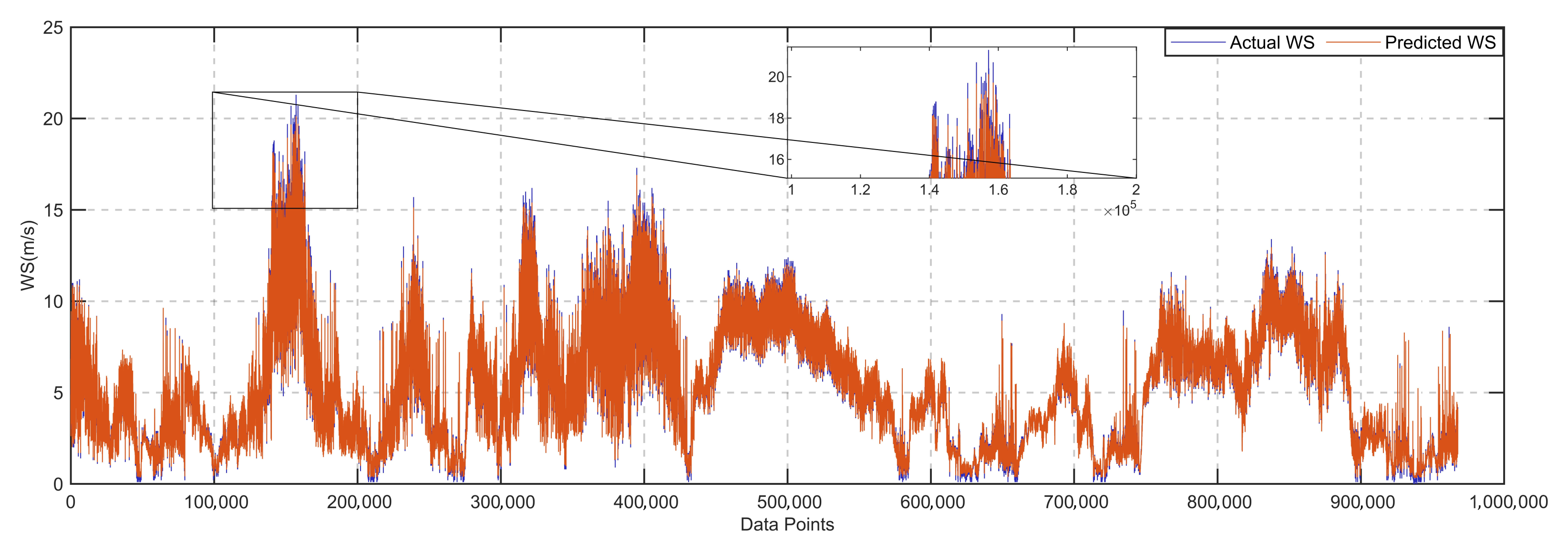
Real WS (label 0)	49	964,611

presents the confusion matrix obtained by the proposed MHSETCN-LSTM model when encoding strong wind events (WS > 15 m/s) as the positive class. The model achieves a prediction accuracy of 99.86%. This indicates that the proposed model can accurately predict the vast majority of WS data. However, the 99.86% prediction accuracy is primarily driven by the imbalanced dataset and is not an effective indicator of strong wind detection quality. The recall of the MHSETCN-LSTM model is only 57.92%, meaning that approximately 42% of strong wind events are not successfully predicted. The low recall is due to the data sample imbalance, with the majority of data points having wind speeds below 15 m/s. The red and blue curves in Figure 6 are highly fitted, indicating that while some strong wind events were not correctly classified, the prediction errors are small. Therefore, the proposed model is a powerful tool for HSR operational decision-making.

4.4. Ablation Analysis

In this section, we perform an ablation analysis to evaluate the contribution of different components of the MHSETCN-LSTM model for both wind speed and wind direction forecasting tasks.

4.4.1. Model Component Ablation

Table 4. Performance evaluation for wind speed forecasting (bold indicates the best; italics indicates the second-best).

Model	MSE	RMSE	${\mathit{R}}^2(\%)$
TCN	3.4475	1.8568	64.00
LSTM	2.9753	1.7249	68.93
TCN-LSTM	0.2545	0.5045	97.34
SETCN-LSTM	0.0441	0.2099	99.54
MHSETCN-LSTM	0.0393	0.1982	99.59

shows the performance evaluation based on different models for wind speed forecasting (WSF). The single TCN model for WSF performs the worst, with an MSE of 3.4475, RMSE of 1.8568, and $R^2$ of 64.00%. This indicates that relying merely on the TCN architecture is insufficient for capturing temporal patterns. The LSTM model achieves an MSE of 2.9753 and an RMSE of 1.7249. It improves the prediction accuracy by capturing long-term dependencies in the time series data due to its unique structure. The TCN-LSTM model, which combines TCN and LSTM, achieves an MSE of 0.2545, RMSE of 0.5045, and $R^2$ of 97.34%. In TCN-LSTM, TCN layers are responsible for short-term fluctuations, while the LSTM layers handle long-term dependencies, offering a substantial improvement over individual components. By further introducing the squeeze-and-excitation (SE) attention mechanism into TCN-LSTM architecture, the SETCN-LSTM achieves an MSE of 0.0441, RMSE of 0.2099, and $R^2$ of 99.54%. The SE attention mechanism enhances the model’s ability to capture complex temporal patterns by dynamically weighting features, allowing the model to focus on the most informative channels.

The performance evaluation of the WD is shown in

Table 5. Performance evaluation for wind direction forecasting (bold indicates the best; italics indicates the second-best).

Model	MSE	RMSE	${\mathit{R}}^2(\%)$
TCN	5825.9559	76.5046	39.01
LSTM	2557.6143	50.5729	74.58
TCN-LSTM	702.0411	26.4961	92.70
SETCN-LSTM	424.9316	20.6139	95.59
MHSETCN-LSTM	391.7053	19.7915	95.92

. The TCN model demonstrates suboptimal performance in predicting WD with an MSE of 5825.9559, RMSE of 76.5046, and $R^2$ of 39.01%. The wind data contain complex spatial and temporal features, and it is difficult to capture the long-term dependence of the wind data by TCN alone. The LSTM model gives prediction results with an MSE of 2557.6143, RMSE of 50.5729, and $R^2$ of 74.58%. Although it outperforms the TCN model, it still faces challenges in capturing the complex patterns of the wind data. By combining TCN with LSTM, the MSE, RMSE, $R^2$ of the TCN-LSTM model is 702.0411, 26.4961, and 92.70%. This improvement is due to the ability of the hybrid model to better handle short-term and long-term dependencies. Compared to those of the TCN-LSTM, the SETCN-LSTM model further improves its performance on all evaluation indicators. The SE attention mechanism helps the model to focus on the most informative features, improving its predictive ability. The MHSETCN-LSTM model achieves the best results in predicting WD, with an MSE of 391.7053, an RMSE of 19.7915, and an $R^2$ of 95.92%.

From Table 4 and Table 5, we found that the MHSETCN-LSTM performance for predicting WD is slightly lower than for predicting WS. The MHSETCN-LSTM model performs slightly worse in predicting WD than WS for several reasons. Firstly, WD is more unstable and harder to predict than WS, especially over shorter time scales. This introduces more noise, which complicates the task of the model and makes it more challenging to detect consistent patterns in the data. In addition, WS is generally a more direct and measurable quantity, whereas WD involves spatial relationships (e.g., the circular nature of angles) and may be more difficult to model directly.

4.4.2. Effect of Module Ordering

To assess the impact of architectural ordering on prediction performance, we conducted comparative experiments on two hybrid model variants: the LSTM-MHSETCN and the MHSETCN-LSTM. As shown in

Table 6. Prediction performance based on different architectural orders.

Model	MSE	RMSE	${\mathit{R}}^2(\%)$
LSTM-MHSETCN	1.2464	1.1164	99.49
MHSETCN-LSTM	0.0393	0.1982	99.59

, the proposed MHSETCN-LSTM model significantly outperforms the LSTM-MHSETCN model across all evaluation metrics. It achieves a lower MSE of 0.0393, a lower RMSE of 0.1982, and a higher $R^2$ of 99.59%. The improved performance is attributed to the well-designed module ordering. When TCN is placed first, it efficiently captures short-term temporal patterns and sharp fluctuations in wind behavior. The subsequent MHSE mechanisms adaptively emphasize key channels and suppress extraneous information, allowing the downstream LSTM to focus more effectively on modeling long-term dependencies without interference from short-term noise. In contrast, in LSTM-MHSETCN, placing the LSTM before the feature recalibration phase tends to mask sudden changes in the input signal, thereby weakening the effect of the MHSE module and reducing the overall prediction performance.

4.4.3. Effect of Trigonometric Transformation for WD

Table 7. The effectiveness of trigonometric transformation on WD representation.

Model	MSE	RMSE	${\mathit{R}}^2(\%)$
Raw WD	470.8095	21.6981	95.12
Trigonometric transformation	391.7053	19.7915	95.92

evaluates the impact of different encoding methods for WD on model performance. Specifically, the experiment compares two configurations of the MHSETCN-LSTM model: one that uses raw angular values of WD and another that employs a trigonometric transformation. All other aspects of the model architecture and training settings remain the same. The results indicate that using trigonometric encoding significantly improves model performance. This improvement can be attributed to the continuous nature of the sine and cosine representation, which removes the artificial discontinuity at angular boundaries and offers a smooth portrayal of WD data. In summary, the MHSETCN-LSTM model provides significant improvements in both WS and WD prediction tasks, but performs slightly worse in WD prediction due to the inherent challenges of predicting more unstable and complex spatio-temporal patterns. However, the model still outperforms traditional methods and provides valuable insight into complex time series forecasting tasks.

4.4.4. Effects of Parallel and Serial Integration

From

Table 8. Prediction performance based on different configurations.

Model	MSE	RMSE	${\mathit{R}}^2(\%)$
Parallel	0.6542	0.8088	87.78
Serial integration	0.0393	0.1982	99.59

, we observe that the serial integration outperforms the parallel integration in terms of MSE, RMSE, and $R^2$. This is because serial integration allows for a more structured flow of information, where short-term features extracted by TCN can be passed to LSTM, which then models the long-term dependencies more effectively. In contrast, parallel integration does not allow for such specialized feature extraction and fusion, leading to suboptimal performance.

4.5. Hyperparameter Sensitivity

In this section, we study the effects of key hyperparameters, including the number of attention heads, reduction ratios, and hidden units. To control variables, we change only one hyperparameter at one time while keeping the other hyperparameters at their optimal values.

4.5.1. Effect of the Number of Attention Heads

To investigate the effect of the number of attention heads in the MHSE module on forecasting performance, we carried out experiments by varying the number of heads while keeping all other components and training configurations constant. The results are summarized in

Table 9. The impact of attention head number in the MHSE module.

Head Number	MSE	RMSE	${\mathit{R}}^2(\%)$
1	0.0441	0.2099	99.54
3	0.0393	0.1982	99.59
5	0.2565	0.5066	97.33

.

The results indicate that the number of attention heads in MHSE plays a critical role in model performance. When using a single attention head, the model achieves reasonable performance, with an MSE 0.0441, an RMSE of 0.2099, and $R^2$ of 99.54%. However, its ability to capture diverse feature dependencies is limited. Using three heads yields the best performance across all metrics, with the lowest RMSE (0.1982) and highest $R^2$ (99.59%), suggesting that multi-head attention facilitates richer feature interactions and improves the model’s sensitivity to abrupt wind variations. However, increasing the number of heads to five results in a notable performance drop. This degradation is due to overparameterization and noise amplification in the attention process, which can lead to feature redundancy and degraded generalization ability. Therefore, we decide to use three heads as the optimal configuration, achieving a good balance between representational power and model stability.

4.5.2. Effect of the Number of Reduction Ratios

To evaluate the performance of our model using different reduction ratios in the MHSE module, we conducted experiments with different sets of reduction ratios. The results are summarized in

Table 10. Performance evaluation for wind speed forecasting using different reduction ratios.

Reduction Ratios	MSE	RMSE	${\mathit{R}}^2(\%)$
$(4,4,4)$	0.3607	0.6006	96.27
$(8,8,8)$	0.5290	0.7252	94.55
$(16,16,16)$	0.6222	0.7888	93.58
$(4,8,16)$	0.0393	0.1982	99.59

. The configuration with mixed reduction rates (4, 8, 16) performs exceptionally well. It achieves significantly lower MSE and RMSE, with a remarkable $R^2$ value of 99.59%, indicating that this combination of reduction rates allows the model to capture dynamic temporal dependencies across multiple scales effectively. By using (4, 8, 16) as the reduction ratios, the model can adaptively focus on different temporal scales, which may explain why this configuration performs best across all evaluation metrics. The performance evaluation confirms that the model with reduction rates (4, 8, 16) in the MHSE module outperforms all other configurations in terms of MSE, RMSE, and $R^2$. The low-error metrics and high $R^2$ indicate that the model successfully captures the temporal dependencies in the wind speed data across various time scales.

4.5.3. Effect of the Number of LSTM Hidden Units

In this experiment, we explored how varying the number of LSTM hidden units affects model performance. We tested several values for the number of hidden units: 8, 16, 32, and 64. The results of these experiments are summarized in

Table 11. Performance evaluation of LSTM with varying hidden unit sizes.

Hidden Units	MSE	RMSE	${\mathit{R}}^2(\%)$
8	0.0415	0.2038	99.56
16	0.0401	0.2003	99.59
32	0.0393	0.1982	99.59
64	0.0473	0.2175	99.50

. The MSE decreased slightly as the number of hidden units increased from 8 (0.0415) to 16 (0.0401) and 32 (0.0393). The RMSE followed the same trend as the MSE. Overall, the differences in performance metrics across various hidden unit sizes were relatively small. The 32 hidden units achieved the best performance, yielding the lowest MSE, the lowest RMSE, and an exceptionally high $R^2$ value of 99.59%.

5. Conclusions

This study proposed the MHSETCN-LSTM framework for strong wind early warning in high-speed railway (HSR) systems. The model combines temporal convolutional networks (TCNs) and long short-term memory (LSTM) networks to effectively capture both short-term and long-term patterns in wind behavior. In addition, we designed a multi-head squeeze-and-excitation (MHSE) attention mechanism, which recalibrates the importance of different components in the input sequence. This capability allows the model to focus on critical time steps, especially during sudden wind events, thereby enhancing the accuracy of wind forecasting. To address the periodic nature of wind direction (WD), we applied a trigonometric transformation that encodes WD as sine and cosine components.

Extensive experiments using real-world wind data collected from the Beijing–Baotou railway confirmed the outstanding performance of our proposed framework:

• The MHSETCN-LSTM model achieved the best predictive performance with an MSE of 0.0393, RMSE of 0.1982, and the highest $R^2$ of 99.59%, outperforming all baseline and ablation variants.
• The ablation experimental results showed that removing the MHSE module significantly increases the MSE and RMSE. This decline in performance confirms that dynamic channel recalibration is essential for accurately forecasting sudden strong wind events.
• The trigonometric representation of WD improved model robustness, reducing the MSE from 470.8095 (raw angle input) to 391.7053.

These improvements in prediction accuracy have practical implications. More reliable WSF allows for more accurate strong wind warnings, which can reduce unnecessary emergency braking and energy expenditure. Hence, the proposed framework contributes not only to the operational safety of HSR systems but also to the broader goals of sustainable transportation. The integration of TCNs, LSTMs, and MHSE attention mechanisms results in increased computational complexity. Future research will focus on improving the speed and efficiency of the model to make it suitable for real-time applications in HSR systems.