Promoting Freight Modal Shift to High-Speed Rail for CO₂ Emission Reduction: A Bi-Level Multi-Objective Optimization Approach

Abstract

This paper investigates the optimal planning of high-speed rail (HSR) freight operations, pricing strategies, and government carbon tax policies. The primary objective is to enhance the market share of HSR freight, thereby reducing carbon dioxide (CO₂) emissions associated with freight activities. The modal shift problem is formulated as a bi-level multi-objective model and solved using a specifically designed hybrid algorithm. The upper-level model integrates multiple objectives of the government (minimizing tax while maximizing the emission reduction rate) and HSR operators (maximizing profits). The lower-level model represents shippers’ transportation mode choices through network equilibrium modeling, aiming to minimize their costs. Numerical analysis is conducted using a transportation network that includes seven major central cities in China. The results indicate that optimizing HSR freight services with carbon tax policies can achieve a 56.97% reduction in CO₂ emissions compared to air freight only. The effectiveness of the government’s carbon tax policy in reducing CO₂ emissions depends on shippers’ emphasis on carbon reduction and the intensity of the carbon tax.

1. Introduction

Logistics emits about 9–10% of global carbon dioxide (CO₂) and is one of the hardest sectors to decarbonize. Freight transportation, driven by complex and interconnected production, trade, and consumption patterns, is one of the most essential and costly activities in the supply chain [1]. Its decarbonization is even more complicated than passenger transport [2]. Shifting freight to rail cuts transport emissions effectively [3]. Since the European Union’s 2011 white paper proposed a 60% cut in transport-related CO₂ emissions by 2050, shifting freight to greener modes has been a key research topic [4]. Numerous studies have focused on different countries and regions, including the European Union [5], Northern Europe [6], Japan [7], the United States [8], China [9], South Korea [10], and India [11].

In recent years, the global demand for high-value-added and time-sensitive express cargo transportation has surged. This trend has been further intensified by the rapid development of e-commerce. The emergence of high-speed rail (HSR) freight has the potential to disrupt the existing express market equilibrium, in which air freight currently holds a significant position. Greenhouse gas emissions from air freight are nearly an order of magnitude higher than those from other transportation modes [12]. In contrast, HSR transportation offers numerous advantages, including high speed, strong safety, large capacity, high punctuality, low emissions, and low energy consumption [13]. Bi et al. [14] suggested that countries such as China, France, Germany, and Japan should leverage the unused capacity in HSR passenger trains to transport express packages. This strategy could increase HSR operating revenue while alleviating the burden on highway and air express transportation.

Table 1. Comparison between HSR and air in express freight.

Feature	HSR	Air
CO2 Emissions	Low	High
Speed	High	Highest
Cost	Moderate	High
Safety	High	High
Capacity	Large	Limited
Punctuality	High	High

presents a comparison of rail and air freight in long-distance transportation.

The limited application of HSR for freight is due to multiple factors. HSR infrastructure is primarily designed for passenger trains and requires modifications to accommodate freight, which can disrupt the efficient operation of HSR networks optimized for passenger services. Additionally, the logistics and supply chain systems in many countries are not fully integrated with HSR networks, hindering seamless pre- and end-haulage services. While speed is important, cost-effectiveness and reliability are equally crucial in logistics systems. Traditional freight modes such as road and conventional rail often provide a better balance of cost and efficiency for most cargo types.

However, HSR freight holds promise in countries with advanced HSR networks and high demand for fast freight services, such as China. China’s high-speed railway mileage has reached 45,000 km, accounting for about 70% of the total global high-speed railway mileage. Since 2014, Chinese railway authorities have been experimenting with HSR freight transport. Currently, there are 293 stations nationwide equipped with HSR freight services, covering all 31 provinces. Supported by government initiatives to modernize the logistics sector and driven by growing market demand for fast, reliable freight services, HSR freight in China shows significant potential. The rapid advancement of China’s logistics industry, with improving supply chain integration and infrastructure, is gradually meeting the conditions for seamless supply chain integration. Furthermore, the Chinese government’s strong support for green transportation initiatives has further propelled the exploration and implementation of HSR freight services.

HSR freight trains encompass two primary types: modified passenger trains and newly developed HSR express freight trains [15]. The modification of passenger trains for freight involves removing seats and luggage racks to create space for parcels. However, this approach has drawbacks such as inefficient parcel loading/unloading and non- professional cargo securing. To enhance HSR freight capabilities, China Railway operates dedicated HSR freight trains that share HSR lines with passenger trains. HSR freight trains are specially designed with large-aperture loading doors, standardized container products, and modular freight-dedicated flooring. These features enable efficient parcel loading/unloading and securing. HSR freight trains can transport parcels swiftly following designated operating patterns, offering significantly better cargo capacity than modified passenger trains.

This research focuses on parcel transportation within the express market. These cargo types are characterized by high-value-added and time-sensitive demands, making them well-suited to HSR transportation. As a relatively new freight mode, HSR still faces organizational challenges in transportation that limit its logistical advantages. To boost HSR freight’s market share, improving its service level in a competitive, liberalized environment is crucial. The government can support the modal shift to HSR by leveraging tax policy tools. By increasing non-clean transport costs, tax policies can enhance cleaner modes’ competitiveness. A key advantage of tax policies is that they allow governments to achieve modal shift targets without extra fiscal spending.

This research introduces a novel bi-level multi-objective optimization model that integrates the optimization of HSR freight operations, HSR freight service pricing, and government carbon tax policies. The model innovatively balances multiple stakeholders’ objectives, including the government’s goals of minimizing taxes and maximizing CO₂ emission reduction rates, as well as HSR operators’ profit maximization goals. Practically, this study provides HSR freight operators with enhanced service decision-making tools to increase market share and profit. It also provides policymakers with insights for effective CO₂ mitigation strategies. Academically, the research addresses a complex multi-stakeholder optimization problem involving the government, carriers, and shippers, and demonstrates how the joint optimization of HSR freight pricing and operation plans can effectively promote the modal shift from air freight to greener HSR freight. Our analysis also reveals that the effectiveness of carbon tax policies in reducing CO₂ emissions depends on both shippers’ emphasis on carbon reduction and the intensity of the carbon tax itself, offering new perspectives for policymakers.

The remainder of this paper is organized as follows. Section 2 reviews the relevant literature. Section 3 presents the methodology, including model establishment and algorithm design. Section 4 undertakes a case study to examine the potential for modal shift engendered by pricing, planning, and taxing strategies. Finally, Section 5 concludes the research.

2. Literature Review

The literature review in this section is divided into two main parts. The first part is problem-oriented, focusing on research related to freight emission reduction, HSR freight operation management, and CO₂ emission reduction policies. The second part is method-oriented, examining the solving algorithms for bi-level multi-objective optimization problems.

Table 2. Overview of literature on reducing CO₂ emissions through modal shift.

Reference	Modal Shift	Measures
Regmi and Hanaoka [16]	Road to rail	Develop a dry port
Wang et al. [17]	Road to intermodal rail transport	Impose a carbon tax on shippers
Bouchery et al. [18]	Road to rail	Control total carbon emissions
Lin et al. [19]	Road to rail	Railway network design
Tao et al. [20]	Road to road–rail combined transport	Fix subsidy to road–rail transport users
Choi, et al. [10]	Road to rail	Containerization and taxation
Kundu and Sheu [21]	Maritime to rail	Subsidy to shippers
Chen et al. [22]	Road to water	Tax subsidy joint policy and regulatory price for water transport
Nassar et al. [23]	Road to rail and water	Infrastructure projects, pricing measures, and stakeholders’ decisions
Masone et al. [24]	Road to rail	Incentives
Takman and Gonzalez-Aregall [25]	Road to rail and water	Subsidies and regulations
Liu and Jia [26]	Road to rail	Subsidy to shippers
This study	Air to HSR	Carbon tax and HSR service optimization

lists studies promoting shifts to greener freight modes and their relevance to this research. Two key findings emerge from Table 2: first, no existing research specifically targets the promotion of modal shift to HSR freight; second, no study has jointly considered the utility equilibrium of the transportation demand side, the operation plan and service pricing of the transportation supply side, and the government’s emission reduction policies.

Subsidy policies have been proven to be valuable tools for controlling greenhouse gas emissions [21,27,28]. They generally increase government fiscal expenditures. In contrast to subsidies, which are based on incentives, carbon tax policies rely on penalties. Wang et al. [17] analyzed the impact of a carbon emission tax on companies’ transportation mode choices and social welfare. They found that a carbon tax can enhance the competitive edge of clean transportation modes. However, it also increases the operating costs and product prices of enterprises, thereby causing social welfare losses. To mitigate these negative impacts, strategies such as tax revenue recycling schemes have been employed. Zhou et al. [29] developed a computable general equilibrium model to simulate the effects of a carbon tax on China’s transportation industry and designed two tax recycling schemes to achieve government revenue neutrality. Qiu et al. [30] proposed a bi-level optimization model to study airline passenger carbon taxes, including both the imposition of carbon taxes and competitive tax rebates for airlines. They also recommended that airlines transfer a portion of the carbon-related costs to passengers.

Research on HSR has predominantly focused on passenger transport [31]. With the construction of HSR network and strong logistics demand, some scholars have started to focus on the use of HSR for transporting goods. Pazour et al. [32] developed an HSR network design model for freight distribution. Their experimental results demonstrated that utilizing HSR for freight transportation can significantly reduce transit times and alleviate traffic congestion on roads. Hoffrichter et al. [33] compared the energy consumption and CO₂ emissions of railway and road vehicles, finding that even in high-speed operation modes, promoting the modal shift to rail can effectively reduce CO₂ emissions. The current operational patterns of HSR freight primarily include the following four types [34]: (1) normal HSR passenger trainsets. (2) piggyback pattern. This pattern utilizes the remaining luggage storage area on HSR passenger trains to transport goods. While it can meet small-scale freight demands, it may negatively impact the passenger experience. (3) the inspecting train. This is the first no-passenger train each day, used to test the safety of HSR tracks. (4) dedicated HSR freight train. This pattern achieves complete separation of freight and passenger transportation. Due to its advantages in capacity, service scope, and economic efficiency, the dedicated HSR freight train has been favored by multiple countries [35]. Zhang et al. [36] analyzed competition between HSR and air transport in passenger and cargo markets, finding that HSR entry solely in the passenger sector might lower social welfare due to limited aircraft belly capacity, yet welfare improved when HSR competed in both sectors. Zhang et al. [37] focused on HSR freight trains from overturning in strong winds. They employed multibody dynamics modeling and gradient-boosting decision tree prediction to optimize cargo distribution, reducing overturning risk by over 10%.

As HSR transportation continues to develop, more research has focused on tactical issues in HSR freight operations, such as train routing and timetable planning. Yu et al. [38] developed a freight operation plan for the Harbin–Dalian HSR in China through a two-stage approach. In the first stage, freight train options were identified to minimize total operating costs. In the second stage, cargo flow was allocated to maximize economic benefits. Subsequently, Yu et al. [39] designed a train diagram for this corridor, considering both the HSR passenger train schedule and the Electric Multiple Unit maintenance plan. Similarly, Jia et al. [15] optimized the number and departure times of freight trains on the Beijing–Xi’an HSR using a bi-level optimization model. The upper level aimed to maximize the railway industry’s profits, while the lower level incorporated the principle of user equilibrium to optimize cargo flow assignment. Li et al. [40] explored HSR freight train rescheduling in large-scale networks. They constructed a candidate train line pool and formulated an integer programming model with 0–1 variables to minimize costs. Wang et al. [41] introduced a joint HSR and crowd–courier system for parcel delivery to address challenges in the express delivery industry. A model was developed to optimize freight allocation and routing. Li et al. [42] investigated the line planning problem for HSR trains to meet passenger and freight demands. Notably, none of these studies considered freight rates. Liang et al. [35] argued that HSR freight rates must be competitive with road and air transportation to attract sufficient freight volume. They highlighted that HSR freight rates are primarily determined by market factors such as competition, supply, and demand.

The literature review on freight emission reduction, HSR freight operation management, and CO₂ emission reduction policies reveals that shifting to eco-friendly modes is a viable solution for reducing freight-related CO₂ emissions. While policy interventions and the optimization of green transport services are recognized as two key measures to facilitate this modal shift, existing research predominantly centers on policies such as carbon taxes and subsidies. However, it fails to sufficiently emphasize the potential of shifting freight to HSR. Additionally, it often overlooks the integrated consideration of multiple stakeholder factors. Research on HSR freight’s feasibility and operation patterns offers evidence of its advantages and potential, laying the foundation for exploring how to optimize carbon tax policies and HSR freight services together to promote modal shift and achieve more significant emission reductions.

In this paper, the bi-level multi-objective optimization method is employed to model the modal shift promotion problem. A bi-level model consists of two optimization problems and features a hierarchical structure. This type of model exhibits two important characteristics: first, it is NP-hard; second, its feasible region is generally non-convex. Multi-objective models are typically transformed into single-objective models through weighting. However, finding appropriate weights for objectives with different units is not a straightforward task. Moreover, this transformation precludes the possibility of obtaining the entire Pareto optimal set, which provides valuable trade-off information between objectives. Bi-level multi-objective optimization is extensively applied in transportation, particularly in Transit Network Design Problems (TNDPs), and is predominantly solved using hybrid heuristic algorithms.

Kolak et al. [43] developed a solution method that integrates Bell’s Second Algorithm, the Self-Regulated Averaging Algorithm, and the Non-dominated Sorted Genetic Algorithm-II (NSGA-II) to address a TNDP from a sustainability perspective. Owais and Osman [44] proposed a comprehensive hierarchical multi-objective genetic algorithm based on NSGA-II to solve a TNDP. Huang et al. [45] devised a solution method that combines a modified successive average method, a modified gradient projection algorithm, and NSGA-II for a sustainable TNDP. These studies demonstrate the widespread application of NSGA-II. However, NSGA-III, with its well-distributed reference points, can maintain better population diversity compared to NSGA-II [46].

The main contributions of this study are as follows: Theoretically, this study analyzes the two-pronged approach to increase the market share of HSR freight, a greener transportation mode. Internally, HSR freight operators integrate operation management and revenue management to optimize their services. Externally, the government enforces a punitive policy to transfer the external costs of CO₂ emissions to shippers. Methodologically, a bi-level multi-objective mixed-integer optimization model is developed to harmonize the goals and constraints of multiple stakeholders. This model integrates operation planning, dynamic pricing, carbon tax optimization, and transportation mode selection. In terms of implementation, a hybrid solution procedure combining NSGA-III, SAB (descent algorithm based on sensitivity analysis), and the CVX 2.1 toolbox is designed. Empirically, numerical analysis is conducted to compare the potential modal shift to HSR, the corresponding CO₂ emission mitigation, and service schemes under different policy scenarios. This analysis provides valuable management insights for reducing CO₂ emissions from transportation activities.

3. Methodology

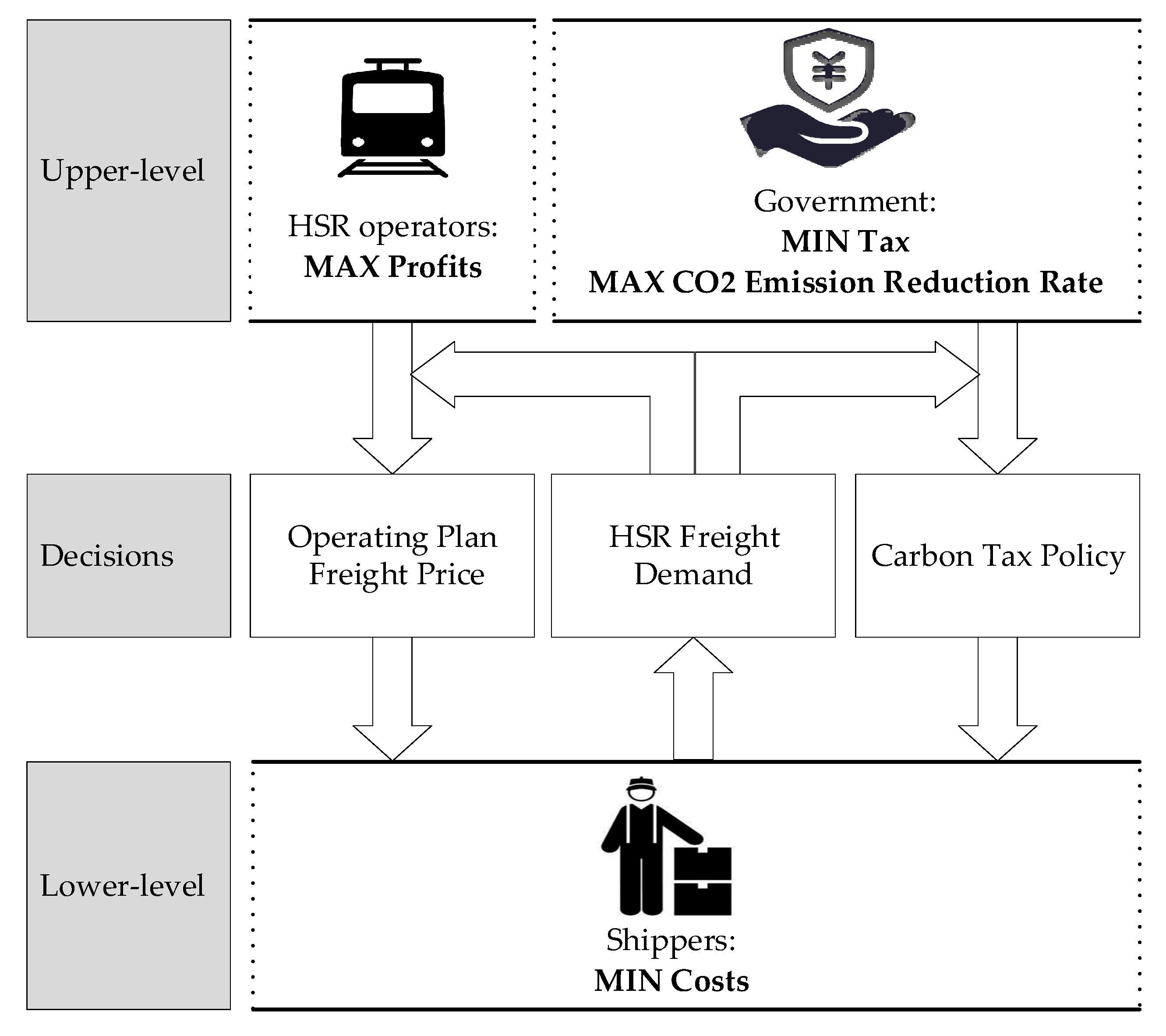
3.1. Problem Description

The purpose of this paper is to enhance the market share of HSR freight by optimizing carbon tax policies, HSR freight rates, and operation plans, thereby reducing CO₂ emissions from freight activities. The overall framework is depicted in Figure 1. The government imposes carbon tax penalties on shippers to internalize external costs. The optimization of HSR freight transportation services influences shippers’ freight mode choices. The decisions of HSR freight operators and the government are shaped by shippers’ flexible transportation demands. This research assumes that HSR operators and the government make decisions simultaneously; hence, both of their decision-making processes are incorporated into the upper-level model.

Table 3. Notations.

Sets:
$\mathbb{S}$	Set of stations in the freight network $\mathbb{S}=\left\{1,2,\dots ,J\right\}$
$\mathbb{W}$	Set of arcs in the freight network $\mathbb{W}=\left\{1,2,\dots ,W\right\}$
$\mathbb{K}$	Set of HSR trains $\mathbb{K}=\left\{1,2,\dots ,K\right\}$
$\mathbb{M}$	Set of express freight transportation mode $\mathbb{M}=\left\{HSR,AIR\right\}$
$\mathbb{Q}$	Set of OD pairs with timeliness requirements $\mathbb{Q}=\left\{Q\left(ij,t\right)\right\}$ , where $Q\left(ij,t\right)$ represents the OD pair from origin $i\in \mathbb{S}$ to destination $j\in \mathbb{S}$ with a timeliness requirement t
Parameters:
${{\displaystyle \sigma }}^m$	Unit CO2 emissions of freight mode $m\in \mathbb{M}$ (tCO2/kg-km)
${{\displaystyle l}}_{ij,t}^m$	Transporting distance of $Q\left(ij,t\right)\in \mathbb{Q}$ to be transported by freight mode $m\in \mathbb{M}$ (km)
$l_k$	Transporting distance of train $k\in \mathbb{K}$ (km)
$l_{ij,t}^k$	Transporting distance of $Q\left(ij,t\right)\in \mathbb{Q}$ to be transported by train $k\in \mathbb{K}$ (km)
$B_{ij,t}$	Total express freight demands of $Q\left(ij,t\right)\in \mathbb{Q}$ (kg)
$c_{fix}^k$	Fixed operating cost of train $k\in \mathbb{K}$ (CNY)
${{\displaystyle c}}_{var}^k$	Distance-related cost of train $k\in \mathbb{K}$ (CNY/km)
$v_m$	The average speed of transportation mode $m\in \mathbb{M}$ (km/h)
$t_{ij,t}^k$	Total transportation time for $Q\left(ij,t\right)\in \mathbb{Q}$ to be transported by train $k\in \mathbb{K}$ (h)
$t_{ij,t}^{1,k}$	In-route transportation time for $Q\left(ij,t\right)\in \mathbb{Q}$ to be transported by train $k\in \mathbb{K}$ (h)
$t_{stop}^k$	Operation time of the train $k\in \mathbb{K}$ at one intermediate station (h)
${\phi }_{stop}^k$	The total number of intermediate station(s) passed by train $k\in \mathbb{K}$
$t_{ij,t}^{1,AIR}$	In-route transportation time for $Q\left(ij,t\right)\in \mathbb{Q}$ to be transported by air freight (h)
$t_{ij,t}^{2,m}$	Station-to-door delivery time for $Q\left(ij,t\right)\in \mathbb{Q}$ to be transported by mode $m\in \mathbb{M}$ (h)
$t_{ij,t}^{3,m}$	Waiting time for $Q\left(ij,t\right)\in \mathbb{Q}$ to be transported by mode $m\in \mathbb{M}$ (h)
$h_{ij,t}^{k,w}$	$h_{k,w}^{ij,t}=1$ if $Q\left(ij,t\right)\in \mathbb{Q}$ is transported by train $k\in \mathbb{K}$ and goes through the arc $w\in \mathbb{W}$ , otherwise $h_{k,w}^{ij,t}=0$
$N_k$	The load capacity of train $k\in \mathbb{K}$ (kg)
$\rho$	Load factor of HSR trains
${{\displaystyle g}}_{w,k}$	${{\displaystyle g}}_{w,k}=1$ if the train $k\in \mathbb{K}$ occupies the transport arc $w\in \mathbb{W}$ , otherwise ${{\displaystyle g}}_{w,k}=0$
${{\displaystyle \xi }}_w$	The passing capacity of the transport arc $w\in \mathbb{W}$
$p_{ij,t}^{\min },p_{ij,t}^{\max }$	Finite constants that denote lower ($p_{ij,t}^{\min }$ ) and upper ($p_{ij,t}^{\max }$ ) bounds for the HSR freight rate of $Q\left(ij,t\right)\in \mathbb{Q}$ (CNY/kg)
${\lambda }_{\min },{\lambda }_{\max }$	Finite constants that denote lower (${\lambda }_{\min }$ ) and upper (${\lambda }_{\max }$ ) bounds for the carbon tax rate (CNY/tCO2)
$f_{ij,t}^m$	Generalized cost of $Q\left(ij,t\right)\in \mathbb{Q}$ to be transported by mode $m\in \mathbb{M}$
$V_{ij,t}^m$	Perceived utility of $Q\left(ij,t\right)\in \mathbb{Q}$ to be transported by mode $m\in \mathbb{M}$
$z_{ij,t}^k$	$z_{ij,t}^k=1$ if $Q\left(ij,t\right)\in \mathbb{Q}$ can be met by train $k\in \mathbb{K}$ , otherwise $z_{ij,t}^k=0$
${\alpha }_1,{\alpha }_2,{\alpha }_3,{\alpha }_4$	Respective weights of the four attributes of freight rate, carbon tax, transportation time, and reliability
Decision variables:
$\lambda$	Carbon tax rate (CNY/tCO2)
$q_{ij,t}^m$	Freight volume of $Q\left(ij,t\right)\in \mathbb{Q}$ that is transported by mode $m\in \mathbb{M}$ (kg)
$p_{ij,t}^{HSR}$	HSR freight rate of $Q\left(ij,t\right)\in \mathbb{Q}$ (CNY/kg)
$q_{ij,t}^k$	Freight volume of $Q\left(ij,t\right)\in \mathbb{Q}$ that is allocated to train $k\in \mathbb{K}$ (kg)
${{\displaystyle \psi }}^k$	Service frequency of train $k\in \mathbb{K}$

provides a summary and explanation of the sets, parameters, and decision variables used in the modeling process.

The model assumes direct rail services without intermediate trans-shipment processes. This assumption simplifies the operational complexity and aligns with the current operational practices of HSR freight systems.

3.2. Upper Level: Decision-Making of the Government and HSR Operators

The following carbon tax optimization model is established to promote freight modal shift from air to HSR and reduce CO₂ emissions from inland express freight activities. The government imposes a carbon tax on shippers to internalize external costs, thereby making cleaner transportation modes more competitive. The resulting carbon tax is presented in Equation (1).

$$G_T(\mathsf{\lambda },\mathit{q})= {\displaystyle \sum _{m\in \mathbb{M}}{\displaystyle \sum _{\left(ij,t\right)\in \mathbb{Q}}\lambda {\sigma }^m{l}_{ij,t}^m{q}_{ij,t}^m}}$$

(1)

CO₂ emissions from the transport system are $E_0$ if all the express freight demands $B_{ij,t}$ are met by air transportation. Let $E$ be the CO₂ emissions after implementing the carbon tax policy and using HSR freight services. The CO₂ emission reduction rate can then be calculated using Equation (4).

$$E_0={\displaystyle \sum _{\left(ij,t\right)\in \mathbb{Q}}{{\displaystyle \sigma }}^{AIR}{B}_{ij,t}{{\displaystyle l}}_{ij,t}^{AIR}}$$

(2)

$$E={\displaystyle \sum _{m\in \mathbb{M}}{\displaystyle \sum _{\left(ij,t\right)\in \mathbb{Q}}{{\displaystyle \sigma }}^m{q}_{ij,t}^m{{\displaystyle l}}_{ij,t}^m}}$$

(3)

$$G_E(\mathit{q})={\displaystyle \frac{E_0-E}{E_0}}$$

(4)

As a form of government revenue, the carbon tax contributes to long-term fiscal sustainability. These tax revenues can be reinvested in measures to reduce CO₂ emissions, such as subsidies for green transportation and the construction of infrastructure with high carbon efficiency. However, excessive taxes may reduce social welfare. Therefore, the government’s objective in this paper is to achieve the optimal CO₂ emission reduction effect with a minimal tax burden, as shown in Equations (5) and (6). Here, $\lambda$ denotes the carbon tax rate to be determined within a specific range.

$$\mathbf{min} G_T(\mathsf{\lambda },\mathit{q})$$

(5)

$$\mathbf{max} G_E(\mathit{q})$$

(6)

$$s.t. {\lambda }_{\min }\le \lambda \le {\lambda }_{\max }$$

(7)

The optimization of HSR freight services in this paper focuses on service frequency, cargo flow assignment, and freight rates. In the process of service optimization, HSR operators aim to maximize their profits. The transportation revenue is calculated as Equation (8). The transportation cost of each HSR express train consists of two components: fixed operating costs and variable costs, as presented in Equation (9).

$$R_I(\mathit{p},\mathit{q})={\displaystyle \sum _{\left(ij,t\right)\in \mathbb{Q}}\left(p_{ij,t}^{HSR}{\displaystyle \sum _{k\in \mathbb{K}}{q}_{ij,t}^k}\right)}$$

(8)

$$R_C(\mathsf{\psi })={\displaystyle \sum _{k\in \mathbb{K}}\left({{\displaystyle c}}_{fix}^k+{{\displaystyle c}}_{var}^k{l}_k\right){{\displaystyle \psi }}^k}$$

(9)

Thus, the objective function of the HSR operators can be expressed as Equation (10), and the following constraints (i)–(v) need to be satisfied.

$$\mathbf{max} R_I(\mathit{p},\mathit{q})-R_C(\mathsf{\psi })$$

(10)

(i)

Constraints on timeliness

Demands in the express market are highly sensitive to the timeliness of transportation services. Meeting timeliness requirements is a fundamental principle in service optimization. Equation (11) specifies that the actual transportation time must not exceed the agreed-upon delivery deadline. In the context of HSR and air freight transportation, pre- and end-haulage typically involves the use of trucks or vans to transport cargo from the origin to the station and from the station to the final destination. Therefore, the HSR transportation time for $Q\left(ij,t\right)$ comprises three parts: in-route transportation time $t_{ij,t}^{1,k}={\displaystyle \frac{l_{ij,t}^k}{v_{HSR}}}+t_{stop}^k{\phi }_{stop}^k$, station-to-door delivery time $t_{ij,t}^{2,HSR}$, and waiting time $t_{ij,t}^{3,HSR}$. The waiting time refers to the period from the goods’ arrival at the station until they are transported. $t_{stop}^k{\phi }_{stop}^k$ represents the total operation time of the train $k$ at all intermediate stations along its route. It is assumed that $t_{stop}^k$, $t_{ij,t}^{2,HSR}$, and $t_{ij,t}^{3,HSR}$ are fixed values.

$$t_{ij,t}^k=t_{ij,t}^{1,k}+t_{ij,t}^{2,HSR}+t_{ij,t}^{3,HSR}\le t,\forall Q\left(ij,t\right)\in \mathbb{Q},\exists k\in \mathbb{K}$$

(11)

(ii)

Constraints on service frequency

Operating an HSR freight train incurs high costs. To ensure the economic viability of HSR operators, the train’s load factor must meet certain requirements. As shown in Figure 2, $q_k^w$ means the freight volume carried by the HSR train $k$ in each arc $w$ on its route ${\mathbb{W}}_k$, which can be determined using Equation (12). Here, ${\mathbb{W}}_k$ denotes the set of arcs that train $k$ traverses. Equation (13) specifies that the freight volume $q_k^w$ on each arc cannot exceed the freight capacity $N_k{{\displaystyle \psi }}^k$. Trains with intermediate loading and unloading have unstable loads. To address this, it is required that a train have a load factor of at least $\rho$ on at least one transportation arc, as indicated in Equation (14).

$$q_k^w={\displaystyle \sum _{\left(ij,t\right)\in \mathbb{Q}}{h}_{ij,t}^{k,w}{q}_{ij,t}^k},\forall k\in \mathbb{K},w\in {\mathbb{W}}_k$$

(12)

$$q_k^w\le N_k{{\displaystyle \psi }}^k,\forall k\in \mathbb{K},w\in {\mathbb{W}}_k$$

(13)

$$\rho N_k{{\displaystyle \psi }}^k\le q_k^w,\forall k\in \mathbb{K},\exists w\in {\mathbb{W}}_k$$

(14)

(iii)

Constraints on the passing capacity of railway arcs

HSR freight trains can only be operated without affecting passenger transportation. To compile an HSR freight train operation plan, it is necessary to fully consider the arc’s passing capacity to ensure its full utilization. The arc capacity constraint, expressed in Equation (15), specifies that the total number of HSR freight trains passing through the same decision period cannot exceed the railway arc’s passing capacity.

$${\displaystyle \sum _{k\in \mathbb{K}}{{\displaystyle g}}_{w,k}{{\displaystyle \psi }}^k}\le {{\displaystyle \xi }}_w,\forall w\in \mathbb{W}$$

(15)

(iv)

Constraints on cargo flow and train flow

The goods are transported directly from the origin station to the destination station without any intermediate transfers. HSR operators need to allocate each HSR transportation demand $q_{ij,t}^{HSR}$ to appropriate trains capable of fulfilling the demand, thereby ensuring that Equation (16) is satisfied. Equation (17) indicates that the HSR train $k$ does not operate (${{\displaystyle \psi }}^k=0$) if no transportation demand is allocated to it (${\displaystyle \sum _{\left(ij,t\right)\in \mathbb{Q}}{q}_{ij,t}^k}=0$), where A is a positive number with a large value.

$${\displaystyle \sum _{k\in \mathbb{K}}{q}_{ij,t}^k}=q_{ij,t}^{HSR},\forall Q\left(ij,t\right)\in \mathbb{Q}$$

(16)

$${{\displaystyle \psi }}^k\le A{\displaystyle \sum _{\left(ij,t\right)\in \mathbb{Q}}{q}_{ij,t}^k},\forall k\in \mathbb{K}$$

(17)

(v)

Constraints on decision variables

Equation (18) defines the permissible range of HSR freight rates. Equation (19) specifies that the freight volume must be non-negative. Equation (20) stipulates that the service frequency must be a non-negative integer.

$$p_{ij,t}^{\min }\le p_{ij,t}^{HSR}\le p_{ij,t}^{\max },\forall Q\left(ij,t\right)\in \mathbb{Q}$$

(18)

$$q_{ij,t}^k\ge 0,\forall Q\left(ij,t\right)\in \mathbb{Q},k\in \mathbb{K}$$

(19)

$${{\displaystyle \psi }}^k\in N,\forall k\in \mathbb{K}$$

(20)

3.3. Lower-Level: Network Equilibrium Model

Under a market economy, changes in HSR freight services and government policies can disrupt the original equilibrium state of cargo flow. Consequently, the cargo flow in the transportation corridor is reallocated among different transportation modes and eventually reaches a new equilibrium state. The equilibrium assignment process reflects the shipper’s choice of transportation mode, aiming to minimize the total generalized cost $f$. The mode choice results can be calculated using the following model [47]:

$$\mathbf{min} {\displaystyle \sum _{m\in \mathbb{M}}{\displaystyle \sum _{Q\left(ij,t\right)\in \mathbb{Q}}{\displaystyle {\int }_0^{q_{ij,t}^m}{f}_{ij,t}^m\left(q\right)d(q)}}}$$

(21)

$$\mathbf{s}\mathbf{.}\mathbf{t}. {\displaystyle \sum _{m\in \mathbb{M}}{q}_{ij,t}^m}=B_{ij,t},\forall Q\left(ij,t\right)\in \mathbb{Q}$$

(22)

$$q_{ij,t}^m\ge 0,\forall Q\left(ij,t\right)\in \mathbb{Q},m\in \mathbb{M}$$

(23)

As shown in Equation (24), the generalized cost $f$ is represented as a power function, which is related to the freight volume and utility. In Equation (25), $V_{ij,t}^m$ represents the transportation utility, a linear function of freight rate $p$, carbon tax $\overline{tax}$, transportation time $\overline{t}$, and reliability $R$. ${\alpha }_1,{\alpha }_2,{\alpha }_3$, and ${\alpha }_4$ are the weights of these four attributes, respectively. The utility function omits the convenience and safety attributes since both air and HSR freight have low cargo damage rates and can provide station-to-door services via road transportation. The transportation reliability is expressed by punctuality rates. Since the same transportation demand $Q\left(ij,t\right)$ may be met by different HSR freight trains, the average transit time $\overline{t}$ and average carbon tax $\overline{tax}$ are used to calculate utility. As shown in Equations (26) and (27), ${\displaystyle \sum _{k\in \mathbb{K}}{z}_{ij,t}^k}$ represents the total number of train services that can satisfy demand $Q\left(ij,t\right)$. The air transportation time of $Q\left(ij,t\right)$ includes three parts: in-route transportation time $t_{ij,t}^{1,AIR}$, station-to-door delivery time $t_{ij,t}^{2,AIR}$, and waiting time $t_{ij,t}^{3,AIR}$.

$$f_{ij,t}^m\left(q\right)=a{\left(q_{ij,t}^m\right)}^b-V_{ij,t}^m,\forall Q\left(ij,t\right)\in \mathbb{Q},m\in \mathbb{M}$$

(24)

$$V_{ij,t}^m=-{\alpha }_1{p}_{ij,t}^m-{\alpha }_2{{\displaystyle \overline{tax}}}_{ij,t}^m-{\alpha }_3{{\displaystyle \overline{t}}}_{ij,t}^m+{\alpha }_4{R}_{ij,t}^m,\forall Q\left(ij,t\right)\in \mathbb{Q},m\in \mathbb{M}$$

(25)

$${{\displaystyle \overline{t}}}_{ij,t}^{HSR}={\displaystyle \frac{{\displaystyle \sum _{k\in \mathbb{K}}{z}_{ij,t}^k{t}_{ij,t}^k}}{{\displaystyle \sum _{k\in \mathbb{K}}{z}_{ij,t}^k}}},\forall Q\left(ij,t\right)\in \mathbb{Q}$$

(26)

$${{\displaystyle \overline{tax}}}_{ij,t}^{HSR}=\lambda {{\displaystyle \sigma }}^{HSR}{\displaystyle \frac{{\displaystyle \sum _{k\in \mathbb{K}}{z}_{ij,t}^k{l}_{ij,t}^k}}{{\displaystyle \sum _{k\in \mathbb{K}}{z}_{ij,t}^k}}},\forall Q\left(ij,t\right)\in \mathbb{Q}$$

(27)

$${{\displaystyle \overline{t}}}_{ij,t}^{AIR}=t_{ij,t}^{1,AIR}+t_{ij,t}^{2,AIR}+t_{ij,t}^{3,AIR},\forall Q\left(ij,t\right)\in \mathbb{Q}$$

(28)

$$t_{ij,t}^{1,AIR}={\displaystyle \frac{l_{ij,t}^{AIR}}{v_{AIR}}},\forall Q\left(ij,t\right)\in \mathbb{Q}$$

(29)

$${{\displaystyle \overline{tax}}}_{ij,t}^{AIR}=\lambda {{\displaystyle \sigma }}^{AIR}{l}_{ij,t}^{AIR},\forall Q\left(ij,t\right)\in \mathbb{Q}$$

(30)

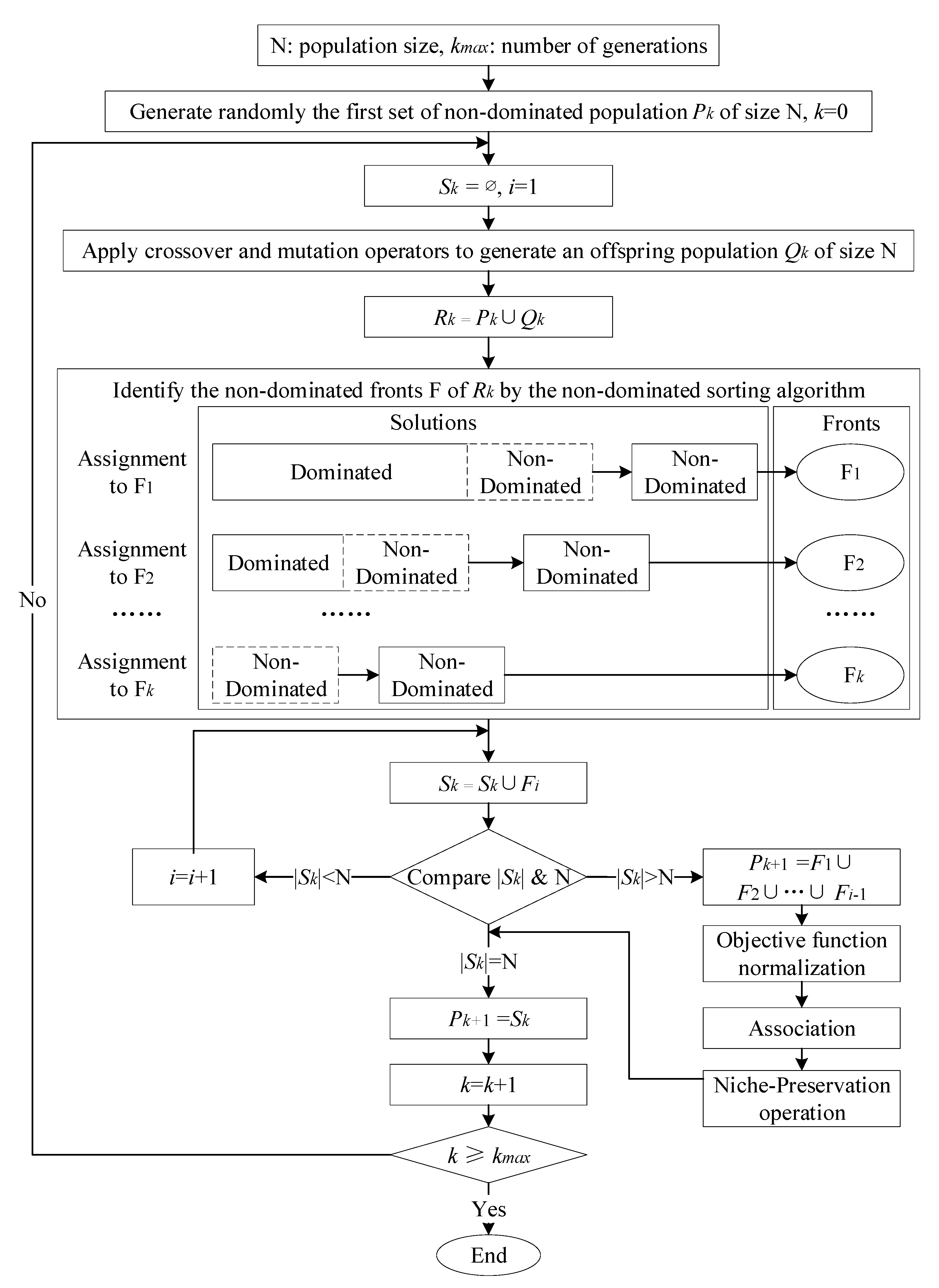
3.4. Algorithm Design

As mentioned in Section 2, the bi-level model is NP-hard. Given this complexity, bi-level multi-objective models are typically solved using hybrid heuristic algorithms. The algorithm framework designed in this paper is presented in Algorithm 1.

Algorithm 1. Pricing, planning, and taxing (PPT) algorithm.

1: Initialize 2:  Set initial parameters: HSR freight rate $p_{ij,t}^{HSR(0)}$ , carbon tax rate ${\lambda }^{(0)}$ 3:  Set relative error threshold err, maximum number of iterations $it{e}_{max}$ 4:  Set iteration counter ite ← 0 5: Repeat 6:  Input $(p_{ij,t}^{HSR(ite)},{\lambda }^{(ite)})$ into lower-level model 7:  Solve lower-level model to obtain equilibrium freight demand $(q_{ij,t}^{HSR(ite)},q_{ij,t}^{AIR(ite)})$ 8:  Update ite ← ite + 1 9:  Find the response function between the freight demand and utility attributes $q_{ij,t}^{HSR(ite)}=f(p_{ij,t}^{HSR},\lambda )$ 10: Substitute $q_{ij,t}^{HSR(ite)}=f(p_{ij,t}^{HSR},\lambda )$ into upper-level model 11:   Solve upper-level model to get updated decision variables: $(p_{ij,t}^{HSR(ite)},q_{ij,t}^{k(ite)},{{\displaystyle \psi }}^{k(ite)},{\lambda }^{(ite)})$ 12: Until    $|p_{ij,t}^{HSR(ite)}-p_{ij,t}^{HSR(ite-1)}|\le err$ or $ite>it{e}_{max}$ 13: Return optimal solution $(p_{ij,t}^{HSR(ite)},q_{ij,t}^{k(ite)},{{\displaystyle \psi }}^{k(ite)},{\lambda }^{(ite)})$

There are three key issues to be resolved in this framework.

(1)

Solving the lower-level model

This model can be addressed using the CVX toolbox, leveraging its convex optimization characteristics.

(2)

Acquiring the reaction function

Let $Ec{o}_{ij,t}^m=-{\alpha }_1{p}_{ij,t}^m-{\alpha }_2{{\displaystyle \overline{tax}}}_{ij,t}^m$. By solving the lower-level model with the initial ${\widetilde{Eco}}_{ij,t}^m$ and other fixed attribute values, the equilibrium HSR freight demand $q_{ij,t}^{HSR}({\widetilde{Eco}}_{ij,t}^m)$ is obtained. The derivative relationship $\partial q/\partial Eco$ is achieved using the sensitivity analysis method. The reaction function is then approximated by a Taylor expansion, as shown in Equation (31).

$$q_{ij,t}^{HSR}(Ec{o}_{ij,t}^m)=q_{ij,t}^{HSR}({\widetilde{Eco}}_{ij,t}^m)+\left[{\displaystyle \frac{\partial q_{ij,t}^{HSR}}{\partial Ec{o}_{ij,t}^{HSR}}},{\displaystyle \frac{\partial q_{ij,t}^{HSR}}{\partial Ec{o}_{ij,t}^{AIR}}}\right]\ast \left[\begin{array}{l}Ec{o}_{ij,t}^{HSR}-{\widetilde{Eco}}_{ij,t}^{HSR}\\ Ec{o}_{ij,t}^{AIR}-{\widetilde{Eco}}_{ij,t}^{AIR}\end{array}\right]$$

(31)

(3)

Solving the upper-level model

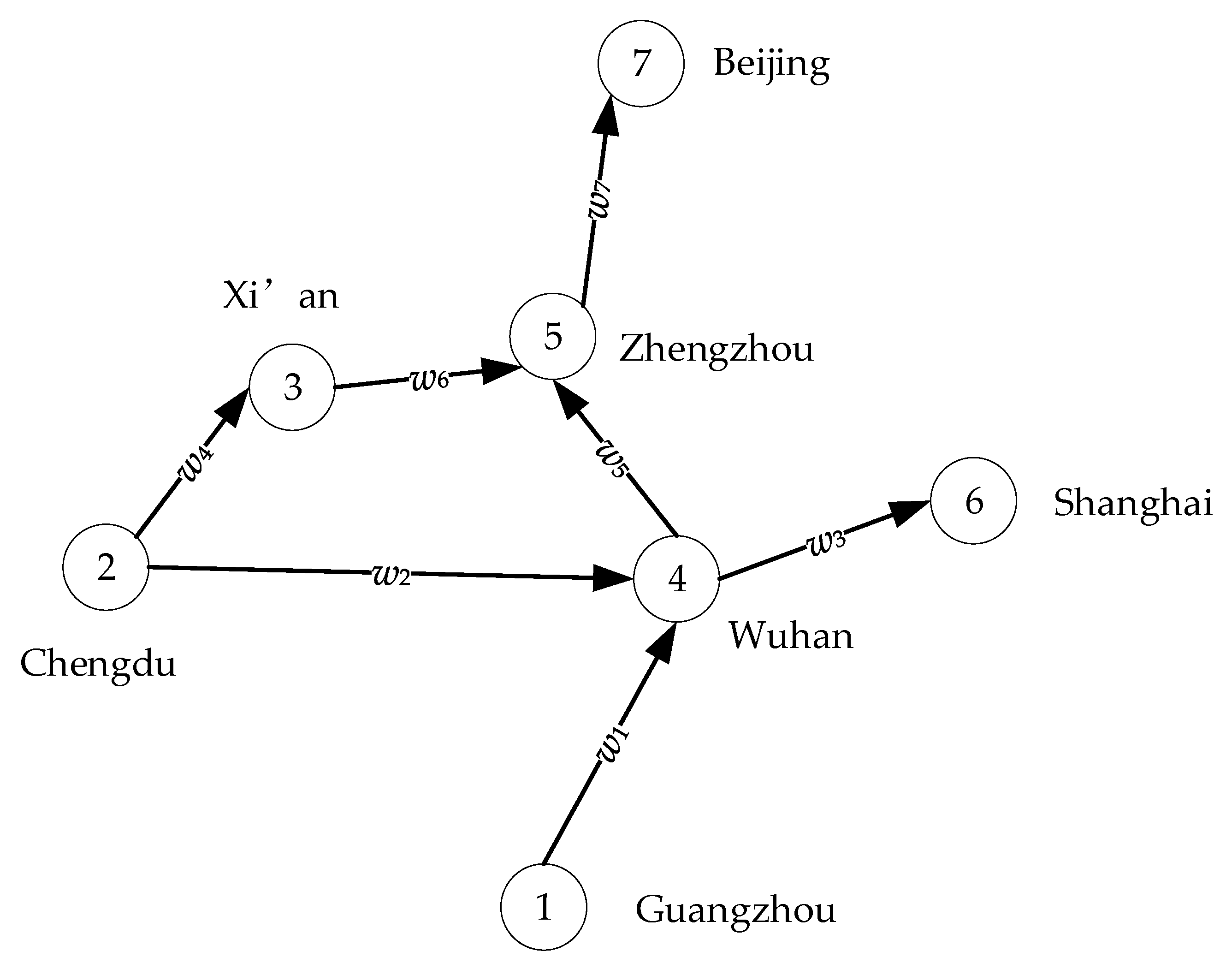
This study employs the metaheuristic method NSGA-III to address the multi-objective problem within the upper-level model. The details of NSGA-III is described in Figure 3 [46]. To facilitate the iteration between the upper-level and lower-level models, the solution with the highest profit for HSR operators is selected from the Pareto front. This solution is regarded as the sole representative of the upper-level multi-objective model.

4. Case Study

4.1. The Input Data

A transportation network encompassing three lines is selected for the case study to validate the proposed methodology: Guangzhou–Wuhan–Zhengzhou–Beijing, Chengdu–Xi’an–Zhengzhou–Beijing, and Chengdu–Wuhan–Shanghai. The network involves seven central cities in China. These cities serve as national comprehensive transportation hubs to some extent. The abstract transportation network is illustrated in Figure 4, featuring 14 transportation ODs.

Currently, HSR freight trains in China consist of fixed groups of eight cars, which cannot be disassembled during operation. The weight of a single car is set at 15 tons. Consequently, the capacity of an eight-car HSR express train is 120 tons. There are seven transportation arcs (see Figure 4): $w_1,w_2,\dots ,w_7$. Their respective HSR distances are [1069, 1149, 820, 658, 483, 505, 631] km.

Table 4. HSR trains and their operating costs.

Train	Route and Stop	Fixed Operating Costs (CNY)	Variable Costs (CNY)
K1	1-4-5-7	420,000	1,309,800
K2	1-(4)-5-7	470,000	1,309,800
K3	1-4-(5)-7	470,000	1,309,800
K4	1-(4)-(5)-7	520,000	1,309,800
K5	2-3-5-7	435,000	1,357,800
K6	2-(3)-5-7	485,000	1,357,800
K7	2-3-(5)-7	485,000	1,357,800
K8	2-(3)-(5)-7	535,000	1,357,800
K9	2-4-6	379,000	1,181,400
K10	2-(4)-6	429,000	1,181,400

presents 10 HSR trains with different operating routes or intermediate stops designed for the case network. Note that the routing sites of train K1 and train K2 are identical. The difference is that K2 stops at station 4, while K1 does not. The same applies to the other trains. The fixed operating costs include station freight service fees, personnel salaries, administrative expenses, and utilities such as water and electricity [38].

The parameter values, such as transportation time and initial freight rates, are provided in

Table 5. Value of parameters.

Parameters	Numerical Value
$N_k$	120 tons
${{\displaystyle \xi }}_w$	20 train
$\rho$	60%
${{\displaystyle c}}_{var}^k$	CNY 600/km
$[v_{HSR},v_{AIR}]$	[250, 600] km/h
$t_{stop}^k$	0.5 h
$[t_{ij,t}^{2,HSR},t_{ij,t}^{2,AIR}]$	[1.5, 1.5] h
$t_{ij,t}^{3,HSR}$	$\left\{\begin{array}{l}1 \mathrm{h},12 \mathrm{h}\mathrm{delivery} \mathrm{and} l_{ij,t}^{HSR}\ge 1600 \mathrm{km}\\ 2 \mathrm{h},12 \mathrm{h}\mathrm{delivery} \mathrm{and} l_{ij,t}^{HSR}\le 1600 \mathrm{km}\\ 11 \mathrm{h}, 24 \mathrm{h}\mathrm{delivery} \mathrm{and} l_{ij,t}^{HSR}\ge 1600 \mathrm{km}\\ 12 \mathrm{h}, 24 \mathrm{h}\mathrm{delivery} \mathrm{and} l_{ij,t}^{HSR}\le 1600 \mathrm{km}\end{array}\right.$
$t_{ij,t}^{3,AIR}$	$\left\{\begin{array}{l}1.5 \mathrm{h},12 \mathrm{h}\mathrm{delivery}\\ 11.5 \mathrm{h},24 \mathrm{h}\mathrm{delivery}\end{array}\right.$
$[R_{ij,t}^{HSR},R_{ij,t}^{AIR}]$	[95%, 76.7%]
$p_{ij,t}^{HSR(0)}$	$\left\{\begin{array}{l}25 \mathrm{CNY}\#/\mathrm{kg},12 \mathrm{h}\mathrm{delivery}\\ 14 \mathrm{CNY}\#/\mathrm{kg}, 24 \mathrm{h}\mathrm{delivery} \mathrm{and} l_{ij,t}^{HSR}\ge 1600 \mathrm{km}\\ 10 \mathrm{CNY}\#/\mathrm{kg}, 24 \mathrm{h}\mathrm{delivery} \mathrm{and} l_{ij,t}^{HSR}\le 1600 \mathrm{km}\end{array}\right.$
$p_{ij,t}^{AIR}$	$\left\{\begin{array}{l}20 \mathrm{CNY}\#/\mathrm{kg},12 \mathrm{h}\mathrm{delivery}\\ 10 \mathrm{CNY}\#/\mathrm{kg},24 \mathrm{h}\mathrm{delivery}\end{array}\right.$
${{\displaystyle [\sigma }}^{HSR},{{\displaystyle \sigma }}^{AIR}]$	[0.0265, 0.6424] kg/ton-km

. As shown in

Table 6. Freight demands, average transit time, and air freight distance.

$\mathit{Q}\left(\mathit{i}\mathit{j},\mathit{t}\right)$	Total Demand (ton)	Average Transit Time (h)		$\mathit{Q}\left(\mathit{i}\mathit{j},\mathit{t}\right)$	Total Demand (ton)	Average Transit Time (h)		Air Freight Distance (km)
		HSR	Air			HSR	Air
(1–4, 12)	183	8	4	(1–4,24)	221	18	14	873
(1–5, 12)	165	10	5	(1–5,24)	192	20	15	1389
(1–7, 12)	439	12	6	(1–7,24)	472	22	16	1967
(4–5, 12)	119	5	4	(4–5,24)	103	15	14	500
(4–7, 12)	277	8	5	(4–7,24)	288	18	15	1133
(5–7, 12)	178	6	4	(5–7,24)	194	16	14	690
(2–3, 12)	63	6	4	(2–3,24)	93	16	14	606
(2–4, 12)	126	8	5	(2–4,24)	120	18	15	1047
(2–5, 12)	119	9	5	(2–5,24)	98	19	15	1039
(2–6, 12)	239	11	6	(2–6,24)	317	21	16	1782
(2–7, 12)	241	12	6	(2–7,24)	313	22	16	1697
(3–5, 12)	62	6	4	(3–5,24)	71	16	14	600
(3–7, 12)	178	8	5	(3–7,24)	162	18	15	936
(4–6, 12)	295	7	4	(4–6,24)	242	17	14	761

, there are 14 transportation demand pairs with two different time requirements (12 h delivery or 24 h delivery). The average transit time is calculated based on Equations (26) and (28). After considering the heterogeneity of shippers with varying timeliness requirements, this research assumes that shippers who require 12 h delivery prioritize transportation time and reliability, followed by price and carbon tax. Their utility function attribute weights are set to $[{\alpha }_1,{\alpha }_2,{\alpha }_3,{\alpha }_4]=[0.2,0.1,0.4,0.3]$. In contrast, shippers with a 24 h delivery requirement place lower weight on transportation time and reliability and higher weight on price and carbon tax compared to those requiring 12 h delivery. Their utility function attribute weights are set to $[{\alpha }_1,{\alpha }_2,{\alpha }_3,{\alpha }_4]=[0.4,0.3,0.2,0.1]$. The parameters of the generalized cost function are set to $[a,b]=[3,0.1]$. The optimizing range of HSR freight rate is set from a 50% decrease to a 15% increase based on the current rates $p_{ij,t}^{HSR(0)}$. Currently, there is limited research on the CO₂ emission intensity of HSR freight. This paper sets the CO₂ emission intensity of HSR freight to 0.0265 kg/ton-km, based on the CO₂ emission intensity of freight trains hauled by electric locomotives. The CO₂ emission intensity of air freight is set to 0.6424 kg/ton-km [48].

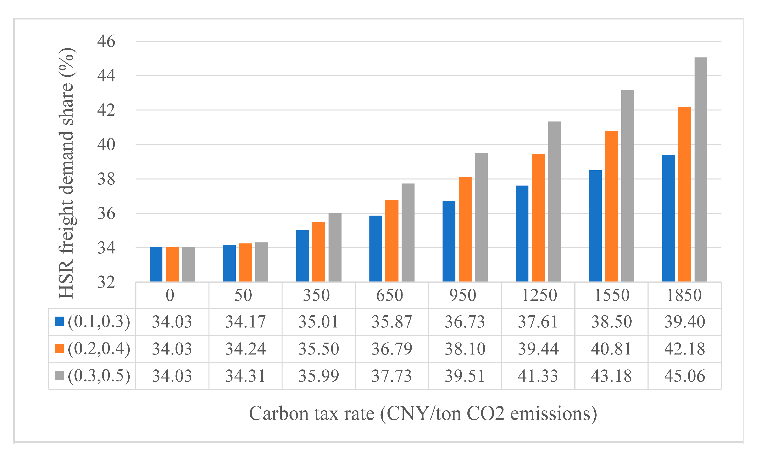
4.2. Results and Discussion

Three scenarios are designed in this section, with their objectives and considerations detailed in

Table 7. Objectives and attributes of Scenario #0–2.

Scenario	Objective(s) of the Upper-Level Model	Attributes in the Lower-Level Model
#0	—	Price, time, reliability
#1	$\mathbf{max} R_I(\mathit{p},\mathit{q})-R_C(\mathsf{\phi },\mathsf{\gamma },\mathsf{\psi })$	Price, time, reliability
#2	$\mathbf{min} G_T(\mathsf{\lambda },\mathit{q})$ $\mathbf{max} G_E(\mathit{q})$ $\mathbf{max} R_I(\mathit{p},\mathit{q})-R_C(\mathsf{\phi },\mathsf{\gamma },\mathsf{\psi })$	Price, carbon tax, time, reliability

.

• Scenario #0: Reference

This scenario serves as a reference. HSR operators implement the current freight rates ($p_{ij,t}^{HSR(0)}$). The government does not impose a carbon tax on shippers. By solving the lower-level model, the respective market share of HSR freight and air freight are obtained.

• Scenario #1: Optimizing HSR freight operation plans and rates

In this scenario, the focus is solely on the modal shift resulting from the optimization of HSR freight rates and operation plans. The government does not participate in decision-making.

• Scenario #2: Tax policy added

Building on Scenario #1, this scenario incorporates the impact of government policy on CO₂ emission reduction. The government imposes a carbon tax on shippers to influence their choice of transportation modes.

The upper-level model of Scenario #2 comprises three objectives. The government aims to impose a low carbon tax to minimize CO₂ emissions, while HSR operators adhere to the principle of profit maximization. By applying the PPT algorithm designed in Section 3.4, the solution to the bi-level multi-objective model can be obtained. Note that solving the multi-objective model in the upper level yields a Pareto optimal solution set.

Table 8. Pareto front of Scenario #2.

No.	Carbon Tax (CNY)	CO2 Emission Reduction Rate	HSR Profits (CNY)
1	55,156	57.080%	6,441,192
2	55,159	57.171%	6,463,972
3	55,341	57.008%	6,465,112
4	55,358	57.046%	6,479,734
5	55,633	57.051%	6,464,437
6	55,976	57.077%	6,466,347
7	56,025	56.973%	6,482,218
8	56,139	57.084%	6,464,309
9	56,337	57.063%	6,471,531

presents the Pareto front at the final iteration—that is, the values of each objective function corresponding to the Pareto optimal solution set. This indicates that the three objectives cannot be simultaneously optimized. For instance, if the carbon tax is reduced, it is not possible for both HSR profits and the CO₂ emission reduction rate to increase concurrently. The detailed decision-making results for Scenarios #0–2 can be found in

Table 9. Optimal HSR freight rates (CNY/kg) for Scenarios #1–2.

$\mathit{Q}\left(\mathit{i}\mathit{j},\mathit{t}\right)$	Scenario			$\mathit{Q}\left(\mathit{i}\mathit{j},\mathit{t}\right)$	Scenario
	#0	#1	#2		#0	#1	#2
(1–4,12)	25	17.55	15.84	(1–4,24)	10	7.71	7.25
(1–5,12)	25	17.71	17.30	(1–5,24)	14	11.11	11.41
(1–7,12)	25	17.78	18.41	(1–7,24)	14	10.20	9.34
(4–5,12)	25	17.86	20.23	(4–5,24)	10	7.64	8.34
(4–7,12)	25	19.42	19.76	(4–7,24)	10	8.65	8.62
(5–7,12)	25	17.04	17.48	(5–7,24)	10	8.16	7.66
(2–3,12)	25	19.13	18.36	(2–3,24)	10	7.71	7.45
(2–4,12)	25	17.56	17.84	(2–4,24)	10	8.14	7.07
(2–5,12)	25	18.60	18.66	(2–5,24)	14	10.46	9.05
(2–6,12)	25	17.98	16.46	(2–6,24)	14	10.00	7.59
(2–7,12)	25	17.03	14.15	(2–7,24)	14	8.45	7.92
(3–5,12)	25	19.57	19.84	(3–5,24)	10	6.95	8.30
(3–7,12)	25	17.99	17.84	(3–7,24)	10	7.68	7.32
(4–6,12)	25	21.23	18.63	(4–6,24)	10	8.18	7.63
Average	25	18.32	17.91	Average	11.43	8.65	8.21

,

Table 10. Optimal HSR freight operation planning for Scenarios #1–2.

Train	Scenario #1			Scenario #2
	Frequency (per Day)	Freight Volume (ton)	Load Factor (%)	Frequency (per Day)	Freight Volume (ton)	Load Factor (%)
K1	1	116.107	96.76	1	118.744	98.95
K2	3	557.724	99.42	3	524.448	99.24
K3	2	293.776	99.67	2	304.135	99.57
K4	3	467.809	99.86	3	536.967	99.89
K5	1	117.479	97.90	1	107.840	89.87
K6	2	304.223	91.17	2	321.312	96.21
K7	1	222.118	91.43	1	248.530	98.15
K8	2	376.613	97.63	2	393.424	99.51
K9	2	212.580	88.58	2	235.905	98.29
K10	3	522.777	99.36	4	653.674	99.76

,

Table 11. Optimal HSR freight market share (%) for Scenarios #0–2.

$\mathit{Q}\left(\mathit{i}\mathit{j},\mathit{t}\right)$	Scenario			$\mathit{Q}\left(\mathit{i}\mathit{j},\mathit{t}\right)$	Scenario
	#0	#1	#2		#0	#1	#2
(1–4,12)	24.03	61.12	69.49	(1–4,24)	46.58	69.51	73.69
(1–5,12)	20.60	56.11	58.33	(1–5,24)	11.91	33.17	30.52
(1–7,12)	19.98	51.21	48.26	(1–7,24)	12.96	40.97	49.46
(4–5,12)	34.50	72.28	60.42	(4–5,24)	53.22	77.03	70.83
(4–7,12)	28.29	55.43	53.77	(4–7,24)	48.75	62.27	62.70
(5–7,12)	31.14	71.49	69.53	(5–7,24)	50.86	69.52	73.88
(2–3,12)	29.28	62.64	66.89	(2–3,24)	50.93	74.88	77.28
(2–4,12)	26.74	65.69	64.33	(2–4,24)	48.63	68.59	78.13
(2–5,12)	23.09	55.94	55.62	(2–5,24)	11.44	41.13	57.13
(2–6,12)	21.45	54.51	62.25	(2–6,24)	13.06	44.61	68.33
(2–7,12)	18.58	55.17	69.27	(2–7,24)	12.02	58.16	63.46
(3–5,12)	29.25	60.15	58.67	(3–5,24)	50.95	81.79	69.91
(3–7,12)	27.43	63.06	63.85	(3–7,24)	48.67	72.20	75.49
(4–6,12)	28.41	46.27	59.38	(4–6,24)	48.72	66.97	71.99
Average	25.91	59.36	61.43	Average	36.34	61.49	65.92

and

Table 12. Summary of simulation outputs.

Results	Scenario #0	Scenario #1	Scenario #2
Carbon tax rate (CNY/tCO2)	—	—	29.11
CO2 emissions (tons)	3437.940	2158.955	1924.742
Average freight rate of HSR (CNY/kg)	18.21	13.48	13.06
Average market share of HSR freight	31.12%	60.42%	63.67%
Modal shift (compare with Scenario #0)	—	29.30%	32.55%
Carbon tax (CNY)	—	—	56,025
CO2 emission reduction rate (compare with air-only)	23.15%	51.74%	56.97%
HSR profits (CNY)	—	7,140,620	6,482,218

. All tests are coded in MATLAB R2018a and executed on a laptop equipped with a 1.80 GHz Intel Core processor and 8 GB of RAM.

The optimally adjusted rates for Scenarios #1 and #2, as shown in Table 9, indicate that a price reduction strategy has been implemented (compared to the current freight rates in Scenario #0). High freight prices negatively impact shippers’ utility. Although environmental considerations are not explicitly addressed in Scenario #1, the implementation of a price reduction strategy demonstrates that HSR operators can maximize their profits by lowering prices to increase freight volume. This strategy in turn leads to a reduction in CO₂ emissions. The HSR freight services are optimized jointly with freight rates and carbon tax strategies. The optimal HSR service frequency, freight volume, and load factor per train are presented in Table 10.

Table 11 presents the HSR freight market share before and after the implementation of pricing, planning, and taxing strategies. It is evident that the proposed methodology significantly increases the market share of HSR freight, regardless of whether it is for 12 h or 24 h delivery. Table 12 summarizes the main output results under the three scenarios. Compared with the reference Scenario #0, Scenario #1, which implements only the joint pricing-planning strategy, achieves a 29.30% modal shift. In Scenario #2, the implementation of the government’s carbon tax policy is expected to make the greener HSR freight more advantageous than air freight. However, HSR profits in Scenario #2 are lower than those in Scenario #1, as HSR operators in Scenario #1 do not consider the government’s strategy, meaning there is only one economic objective in the upper-level model.

From Table 12, it is evident that the additional contribution of the carbon tax policy to increasing the market share of HSR is not significantly better than the service optimization strategy alone. One possible reason is the relatively low carbon tax. In the above discussion, the government implements a carbon tax within the range of [0, 100] CNY/tCO₂, which represents a small cost relative to the shipper’s transportation price. For example, the current transportation price for 1 kg of cargo Q(1−7,12) by HSR is 25 CNY, while the carbon tax, calculated at a rate of 100 CNY/tCO₂, amounts to only 0.0058 CNY. Another possibility is that shippers place less emphasis on green transportation, as reflected in the weight assigned to the carbon tax attribute in the shipper’s utility function. As previously discussed, the weights assigned to the carbon tax attribute for 12 h and 24 h delivery are set to (0.1, 0.3), respectively. The changes in HSR freight demand under different carbon tax weights and intensities, obtained through the lower-level model, corroborate these two possible reasons, as illustrated in Figure 5.

The experiment of Scenario #2 is repeated in three combinations: low carbon tax with high carbon tax weight, high carbon tax with low carbon tax weight, and high carbon tax with high carbon tax weight. The results are presented in

Table 13. Results of Scenario #2 under different carbon tax rates and weights.

Item	Results
$({\lambda }_{\min },{\lambda }_{\max })$	(0, 100)	(1800, 1900)	(1800, 1900)
$({\alpha }_2^{12-h},{\alpha }_2^{24-h})$	(0.3, 0.5)	(0.1, 0.3)	(0.3, 0.5)
Carbon tax rate (CNY/tCO2)	20.67	1844.81	1850.65
CO2 emissions (ton)	1941.106	1668.259	1407.869
Average freight rate of HSR (CNY/kg)	12.92	13.44	13.10
Average market share of HSR freight	64.06%	66.51%	73.41%
Modal shift (compare with Scenario #0 in Section 4.2)	32.94%	35.39%	42.29%
Carbon tax (CNY)	40,116	3,077,627	2,605,473
CO2 reduction rate (compare with air-only)	56.61%	62.71%	68.53%
HSR profits (CNY)	6,687,611	6,786,794	6,644,680

. The combination of high carbon tax and high priority for carbon tax achieves the most significant CO₂ emission reduction effect. The government can increase shippers’ focus on low-emission transportation through publicity or by implementing high carbon taxes. It is noted that even with a high emphasis on green transportation, a low carbon tax hardly achieves a better modal shift. One possible solution is to return the carbon tax to shippers through certain mechanisms, preferably in a manner related to CO₂ emissions. How to reuse the carbon tax is an interesting area for further exploration. For example, Chang et al. [49] reused the road transport tax for water transport subsidy policies, thereby reducing regional CO₂ emissions with minimal investment. Developing a policy package to reuse the carbon tax requires a trade-off decision among fiscal expenditure, social welfare, and CO₂ emissions.

5. Conclusions

To reduce CO₂ emissions from cargo transportation activities, it is essential to guide shippers toward choosing HSR, which is a greener alternative to air freight. The participation of three stakeholders is considered in the decision-making process, and bi-level programming is employed for modeling. The upper-level model is established with multiple objectives: the government aims to minimize taxes and maximize the emission reduction rate, while HSR operators seek to maximize profits. The lower-level model represents shippers’ transportation mode choices through network equilibrium modeling, aiming to minimize their costs. To solve this model, the PPT algorithm is designed, which integrates NSGA-III, SAB, and the CVX toolbox. To test the methodology’s effectiveness for modal shift and CO₂ reduction, multiple comparative scenarios are designed for numerical analysis using a transportation network composed of seven central cities in China.

In a competitive market environment, the joint optimization of HSR freight pricing and operation plans is beneficial for capturing a larger market share. This strategy is crucial for enhancing transportation profits and can significantly contribute to reducing CO₂ emissions from transportation activities. Nevertheless, the effectiveness of the government’s carbon tax policy in reducing emissions cannot be generalized and depends on two factors: shippers’ sensitivity to the carbon tax and the intensity of the carbon tax itself. Taking Scenario #0 as the comparison benchmark, when both the carbon tax and shippers’ carbon tax weight are low, a 32.55% modal shift can be achieved through carbon tax and HSR service optimization, resulting in a reduction in CO₂ emissions of 1513.198 tons. If a high carbon tax is paired with a low carbon tax weight, the modal shift increases to 35.39%, with CO₂ emissions decreasing by 1769.681 tons. Furthermore, combining a high carbon tax with a high carbon tax weight can lead to an additional reduction in CO₂ emissions of 260.390 tons. However, when the carbon tax is low, the effect of a high carbon tax weight on emissions reduction is rather limited.

Future research could explore several key directions. Firstly, service efficiency can be enhanced by focusing on minimizing transportation waiting times in the scheduling of HSR freight services. Waiting times have a significant impact on total transportation time and costs, thereby influencing shippers’ mode choices and the overall efficiency of the freight system. For example, by analyzing historical freight data and market trends, and incorporating modern technologies such as machine learning, more accurate freight demand forecasts can be carried out across different regions and periods. This enables better alignment of freight capacity with demand. Additionally, developing methods to strengthen the integration and coordination between HSR freight and other transportation modes can reduce transfer waiting times and improve the efficiency of the entire freight system. This could involve creating multimodal transport hubs and information-sharing platforms to enable seamless cargo transfers.

Secondly, the exploration of carbon tax recycling mechanisms is crucial. By strategically recycling carbon tax revenue—such as subsidizing green transportation initiatives or investing in carbon-efficient infrastructure—a positive feedback loop can be created to further reduce regional CO₂ emissions. This approach provides a more comprehensive policy design perspective, helping to balance fiscal expenditure, social welfare, and CO₂ emission reductions. For instance, a portion of the carbon tax revenue could be allocated to subsidizing HSR freight infrastructure development or to supporting research and innovation in emission reduction technologies. This would not only enhance the competitiveness of HSR freight services but also advance the sustainability of the transportation sector as a whole.

Thirdly, collecting empirical data on HSR freight carbon emissions, especially regarding different electricity sources, would enhance the accuracy of emission calculations. This includes examining how green versus grey electricity affects the environmental benefits of HSR freight. Such research could provide a more accurate and comprehensive view of the carbon footprint of HSR freight operations and help in formulating more effective emission reduction strategies.

References

1. Pathak, D.K.; Thakur, L.S.; Rahman, S. Performance evaluation framework for sustainable freight transportation systems. Int. J. Prod. Res. 2019, 57, 6202–6222. [Google Scholar] [CrossRef]
2. Marcucci, E.; Gatta, V.; Le Pira, M.; Elias, W. Modal shift, emission reductions and behavioral change: Transport policies and innovations to tackle climate change. Res. Transp. Econ. 2019, 73, 1–3. [Google Scholar] [CrossRef]
3. Kaack, L.H.; Vaishnav, P.; Morgan, M.G.; Azevedo, I.L.; Rai, S. Decarbonizing intraregional freight systems with a focus on modal shift. Environ. Res. Lett. 2018, 13, 083001. [Google Scholar] [CrossRef]
4. Raza, Z.; Svanberg, M.; Wiegmans, B. Modal shift from road haulage to short sea shipping: A systematic literature review and research directions. Transp. Rev. 2020, 40, 382–406. [Google Scholar] [CrossRef]
5. Islam, D.M.Z.; Ricci, S.; Nelldal, B.-L. How to make modal shift from road to rail possible in the European transport market, as aspired to in the EU Transport White Paper 2011. Eur. Transp. Res. Rev. 2016, 8, 18. [Google Scholar] [CrossRef]
6. Salvucci, R.; Gargiulo, M.; Karlsson, K. The role of modal shift in decarbonising the Scandinavian transport sector: Applying substitution elasticities in TIMES-Nordic. Appl. Energy 2019, 253, 113593. [Google Scholar] [CrossRef]
7. Mizutani, J.; Fukuda, S. Issues on modal shift of freight from road to rail in Japan: Review of rail track ownership, investment and access charges after the National Railway restructuring. Res. Transp. Bus. Manag. 2020, 35, 100484. [Google Scholar] [CrossRef]
8. Bickford, E.; Holloway, T.; Karambelas, A.; Johnston, M.; Adams, T.; Janssen, M.; Moberg, C. Emissions and Air Quality Impacts of Truck-to-Rail Freight Modal Shifts in the Midwestern United States. Environ. Sci. Technol. 2014, 48, 446–454. [Google Scholar] [CrossRef]
9. Chen, S.; Wu, J.; Zong, Y. The Impact of the Freight Transport Modal Shift Policy on China’s Carbon Emissions Reduction. Sustainability 2020, 12, 583. [Google Scholar] [CrossRef]
10. Choi, B.; Park, S.-i.; Lee, K.-D. A System Dynamics Model of the Modal Shift from Road to Rail: Containerization and Imposition of Taxes. J. Adv. Transp. 2019, 2019, 7232710. [Google Scholar] [CrossRef]
11. Chandra, S.; Christiansen, M.; Fagerholt, K. Analysing the modal shift from road-based to coastal shipping-based distribution—A case study of outbound automotive logistics in India. Marit. Policy Manag. 2020, 47, 273–286. [Google Scholar] [CrossRef]
12. To, W.M. Greenhouse gases emissions from the logistics sector: The case of Hong Kong, China. J. Clean. Prod. 2015, 103, 658–664. [Google Scholar] [CrossRef]
13. Chai, J.; Zhou, Y.; Zhou, X.; Wang, S.; Zhang, Z.G.; Liu, Z. Analysis on shock effect of China’s high-speed railway on aviation transport. Transp. Res. Part A-Policy Pract. 2018, 108, 35–44. [Google Scholar] [CrossRef]
14. Bi, M.; He, S.; Xu, W. Express delivery with high-speed railway: Definitely feasible or just a publicity stunt. Transp. Res. Part A-Policy Pract. 2019, 120, 165–187. [Google Scholar] [CrossRef]
15. Jia, X.; He, R.; Chai, H. Optimizing the Number of Express Freight Trains on a High-speed Railway Corridor by the Departure Period. IEEE Access 2020, 8, 100058–100072. [Google Scholar] [CrossRef]
16. Regmi, M.B.; Hanaoka, S. Assessment of Modal Shift and Emissions along a Freight Transport Corridor Between Laos and Thailand. Int. J. Sustain. Transp. 2015, 9, 192–202. [Google Scholar] [CrossRef]
17. Wang, M.; Liu, K.; Choi, T.-M.; Yue, X. Effects of Carbon Emission Taxes on Transportation Mode Selections and Social Welfare. IEEE Trans. Syst. Man Cybern.—Syst. 2015, 45, 1413–1423. [Google Scholar] [CrossRef]
18. Bouchery, Y.; Ghaffari, A.; Jemai, Z.; Fransoo, J. Sustainable transportation and order quantity: Insights from multiobjective optimization. Flex. Serv. Manuf. J. 2016, 28, 367–396. [Google Scholar] [CrossRef]
19. Lin, B.; Liu, C.; Wang, H.; Lin, R. Modeling the railway network design problem: A novel approach to considering carbon emissions reduction. Transport. Res. Part D-Transport. Environ. 2017, 56, 95–109. [Google Scholar] [CrossRef]
20. Tao, X.; Wu, Q.; Zhu, L. Mitigation potential of CO2 emissions from modal shift induced by subsidy in hinterland container transport. Energy Policy 2017, 101, 265–273. [Google Scholar] [CrossRef]
21. Kundu, T.; Sheu, J.-B. Analyzing the effect of government subsidy on shippers’ mode switching behavior in the Belt and Road strategic context. Transp. Res. Part E-Logist. Transp. Rev. 2019, 129, 175–202. [Google Scholar] [CrossRef]
22. Chen, K.; Xin, X.; Niu, X.; Zeng, Q. Coastal transportation system joint taxation-subsidy emission reduction policy optimization problem. J. Clean. Prod. 2020, 247, 119096. [Google Scholar] [CrossRef]
23. Nassar, R.F.; Ghisolfi, V.; Annema, J.A.; van Binsbergen, A.; Tavasszy, L.A. A system dynamics model for analyzing modal shift policies towards decarbonization in freight transportation. Res. Transp. Bus. Manag. 2023, 48, 100966. [Google Scholar] [CrossRef]
24. Masone, A.; Marzano, V.; Simonelli, F.; Sterle, C. Exact and heuristic approaches for the Modal Shift Incentive Problem. Socio-Econ. Plan. Sci. 2024, 93, 101874. [Google Scholar] [CrossRef]
25. Takman, J.; Gonzalez-Aregall, M. Public policy instruments to promote freight modal shift in Europe: Evidence from evaluations. Transp. Rev. 2024, 44, 612–633. [Google Scholar] [CrossRef]
26. Liu, S.; Jia, G.Z. Promoting the modal shift of freight from road to rail in China: An evolutionary game and simulation study. PLoS ONE 2025, 20, e0320880. [Google Scholar] [CrossRef]
27. Qu, C.; Wang, G.W.Y.; Zeng, Q. Modelling port subsidy policies considering pricing decisions of feeder carriers. Transp. Res. Part E-Logist. Transp. Rev. 2017, 99, 115–133. [Google Scholar] [CrossRef]
28. Jiang, Y.; Sheu, J.-B.; Peng, Z.; Yu, B. Hinterland patterns of China Railway (CR) express in China under the Belt and Road Initiative: A preliminary analysis. Transp. Res. Part E-Logist. Transp. Rev. 2018, 119, 189–201. [Google Scholar] [CrossRef]
29. Zhou, Y.; Fang, W.; Li, M.; Liu, W. Exploring the impacts of a low-carbon policy instrument: A case of carbon tax on transportation in China. Resour. Conserv. Recycl. 2018, 139, 307–314. [Google Scholar] [CrossRef]
30. Qiu, R.; Xu, J.; Xie, H.; Zeng, Z.; Lv, C. Carbon tax incentive policy towards air passenger transport carbon emissions reduction. Transport. Res. Part D-Transport. Environ. 2020, 85, 102441. [Google Scholar] [CrossRef]
31. Xia, W.; Zhang, A. High-speed rail and air transport competition and cooperation: A vertical differentiation approach. Transp. Res. Part B-Methodol. 2016, 94, 456–481. [Google Scholar] [CrossRef]
32. Pazour, J.A.; Meller, R.D.; Pohl, L.M. A model to design a national high-speed rail network for freight distribution. Transp. Res. Part A-Policy Pract. 2010, 44, 119–135. [Google Scholar] [CrossRef]
33. Hoffrichter, A.; Silmon, J.; Iwnicki, S.; Hillmansen, S.; Roberts, C. Rail freight in 2035-traction energy analysis for high-performance freight trains. Proc. Inst. Mech. Eng. Part F-J. Rail Rapid Transit 2012, 226, 568–574. [Google Scholar] [CrossRef]
34. Liang, X.-H.; Tan, K.-H. Market potential and approaches of parcels and mail by high speed rail in China. Case Stud. Transp. Policy 2019, 7, 583–597. [Google Scholar] [CrossRef]
35. Liang, X.-H.; Tan, K.-H.; Whiteing, A.; Nash, C.; Johnson, D. Parcels and mail by high speed rail—A comparative analysis of Germany, France and China. J. Rail Transp. Plan. Manag. 2016, 6, 77–88. [Google Scholar] [CrossRef]
36. Zhang, Y.D.; Hu, R.; Chen, R.T.; Cai, D.L.; Jiang, C.M. Competition in cargo and passenger between high-speed rail and airlines-considering the vertical structure of transportation. Transp. Policy 2024, 151, 120–133. [Google Scholar] [CrossRef]
37. Zhang, D.; Zhou, F.-R.; Ao, W.K.; Guo, Z.-H.; Chen, Z.-W. Optimization of cargo distribution for high-speed freight trains to overcome strong wind conditions. Eng. Appl. Comput. Fluid Mech. 2024, 18, 2434008. [Google Scholar] [CrossRef]
38. Yu, X.; Lang, M.; Gao, Y.; Wang, K.; Su, C.-H.; Tsai, S.-B.; Huo, M.; Yu, X.; Li, S. An Empirical Study on the Design of China High-Speed Rail Express Train Operation Plan-From a Sustainable Transport Perspective. Sustainability 2018, 10, 2478. [Google Scholar] [CrossRef]
39. Yu, X.; Lang, M.; Zhang, W.; Li, S.; Zhang, M.; Yu, X. An Empirical Study on the Comprehensive Optimization Method of a Train Diagram of the China High Speed Railway Express. Sustainability 2019, 11, 2141. [Google Scholar] [CrossRef]
40. Li, S.; Zuo, D.; Li, W.; Zhang, Y.; Shi, L. Freight train line planning for large-scale high-speed rail network: An integer Benders decomposition-based branch-and-cut algorithm. Transp. Res. Part E-Logist. Transp. Rev. 2024, 192, 103750. [Google Scholar] [CrossRef]
41. Wang, X.; Zhen, L.; Wang, S. Optimizing an express delivery mode based on high-speed railway and crowd-couriers. Transp. Policy 2024, 159, 157–177. [Google Scholar] [CrossRef]
42. Li, S.; Chen, X.; Lang, M. A hybrid heuristic algorithm for high-speed rail line planning problem with multiple transport organization modes. Res. Transp. Bus. Manag. 2025, 60, 01949969. [Google Scholar] [CrossRef]
43. Kolak, O.I.; Feyzioglu, O.; Noyan, N. Bi-level multi-objective traffic network optimisation with sustainability perspective. Expert Syst. Appl. 2018, 104, 294–306. [Google Scholar] [CrossRef]
44. Owais, M.; Osman, M.K. Complete hierarchical multi-objective genetic algorithm for transit network design problem. Expert Syst. Appl. 2018, 114, 143–154. [Google Scholar] [CrossRef]
45. Huang, W.; Xu, G.; Lo, H.K. Pareto-Optimal Sustainable Transportation Network Design under Spatial Queuing. Netw. Spat. Econ. 2020, 20, 637–673. [Google Scholar] [CrossRef]
46. Deb, K.; Jain, H. An Evolutionary Many-Objective Optimization Algorithm Using Reference-Point-Based Nondominated Sorting Approach, Part I: Solving Problems With Box Constraints. IEEE Trans. Evol. Comput. 2014, 18, 577–601. [Google Scholar] [CrossRef]
47. Sheffi, Y. Urban Transportation Networks: Equilibrium Analysis with Mathematical Programming Methods; Prentice-Hall: Englewood Cliffs, NJ, USA, 1984. [Google Scholar]
48. Chao, C.-C. Assessment of carbon emission costs for air cargo transportation. Transport. Res. Part D-Transport. Environ. 2014, 33, 186–195. [Google Scholar] [CrossRef]
49. Chang, X.; Wu, J.; Li, T.; Fan, T.-J. The joint tax-subsidy mechanism incorporating extended producer responsibility in a manufacturing-recycling system. J. Clean. Prod. 2019, 210, 821–836. [Google Scholar] [CrossRef]
Figure 1. Model framework.
Sustainability 17 06310 g001
Figure 2. A schematic diagram of a freight train passing through three arcs.
Sustainability 17 06310 g002
Figure 3. Flowchart of NSGA-III.
Sustainability 17 06310 g003
Figure 4. The abstract transportation network.
Sustainability 17 06310 g004
Figure 5. HSR freight demand share under different carbon tax rate and weight.
Sustainability 17 06310 g005