1. Introduction
The water conservancy projects constructed in the cold regions at high latitudes around the world (such as Northern Europe, Canada, the Qinghai-Tibet Plateau, etc.) face multiple challenges during the dry season, including reduced water inflow, complex ice conditions, and ecological sensitivity. In this context, the research on reservoir operation in high-latitude cold regions is transitioning from traditional flood control safety to multi-objective collaborative management. The operation strategies of these reservoirs directly affect regional water supply security, energy stability, and cross-border ecological balance. Consequently, research on reservoir operation in high-latitude cold regions is shifting from a traditional focus on flood control safety towards multi-objective, collaborative management. These reservoirs’ operational strategies directly impact regional water supply security, energy stability, and cross-border ecological balance. Zhang et al. [
1] conducted a study on two cross-border reservoirs located at the border between China and Laos, which have typical tropical climate characteristics. They proposed a scheduling strategy of releasing 100% of the natural flow during the dry season to cope with drought. Eventually, it was concluded that the reservoirs could alleviate drought by regulating the runoff during the dry season. However, Weber et al. [
2] noted that such regulation may reduce dissolved oxygen levels in downstream water, particularly in deeper layers, potentially harming aquatic ecosystems. The Danjiangkou Reservoir is located in central China and has a climate of northern subtropical monsoon. Xu et al. [
3] conducted research on the Danjiangkou Reservoir and proposed that the operation of the reservoir needs to balance the demand for power generation and ecological flow. By optimizing the scheduling plan, the ecological and social economic benefits can be increased by 9.4–16.4% in drought years. Reservoir operation during low-flow periods in cold regions is complex, largely because of ice conditions. Therefore, it requires balancing refined hydrological control with climate change adaptation. Future research should focus on interdisciplinary collaboration and the development of intelligent management tools.
The HEC-RAS model is hydraulic analysis software developed by the U.S. Army Corps of Engineers. Its full name is the Hydrological Engineering Center-River Analysis System (HEC-RAS). This model can perform water surface profile calculations for various hydraulic structures, including bridges, culverts, weirs, flood levees, and reservoirs. The model also generates various analysis results, including charts and graphs such as cross-section profiles, flow and stage hydrographs, and 3D cross-sectional views of composite channels. Furthermore, the model can analyze river networks within the study area to support flood inundation hazard assessments. Current research utilizing the HEC-RAS model primarily focuses on reservoir dam-break risk analysis and flood inundation assessment. In Erbil, Iraq, Kanal et al. [
4] successfully assessed flood sensitivity and vulnerability by integrating soil maps, land use data, and Digital Elevation Model (DEM) data using the HEC-RAS 2D model. They also investigated the impact of different DEM resolutions on the model results. Namgyal et al. [
5] utilized the HEC-RAS model to analyze future flow patterns at Hirakud Reservoir under CMIP6 climate change scenarios and assess the consequences of a dam-break. They also identified potential downstream inundation areas and changes in water depth. Furthermore, the HEC-RAS model can overcome the limitations of standalone models through coupling with other models. Mustafa A. et al. [
6] simulated hydrodynamics and water quality parameters of the Bokha Stream by coupling SWAT with HEC-RAS and assessed fish habitat suitability. Chang et al. [
7] investigated the integration of the HEC-RAS and Qual2kw models, analyzing hydrodynamic and environmental parameters related to heavy metal transport. Jiang et al. [
8] achieved precise simulation of the spatiotemporal dynamics of urban flooding using an integrated model that couples SWMM with HEC-RAS 2D. This integrated model automatically transmits node flood discharge rates to calculate changes in water depth and velocity.
Although the HEC-RAS model is widely used for flood simulation, river channel restoration planning, and water resources management, limited research has focused on supply regulation and assurance during low-flow periods in high-latitude cold-region reservoirs. Previous studies indicate that the runoff recession rate during the frozen period in the northeastern high-latitude cold region can be as high as 40–60%. Adding to these challenges are stringent ecological flow constraints, leading to a significant conflict for high-latitude cold-region reservoirs between ensuring a stable water supply and protecting the ecological system/chain. Traditional HEC-RAS models primarily simulate flow-stage relationships for individual elements; however, the dynamic adjustment of spillway crest elevations, the operational scheduling (or closure curves) of water intakes, and the overall coordination mechanism for reservoir storage regulation in cold-region reservoir projects remain largely unquantified. Meanwhile, considering characteristics such as the long frozen period in the northeastern cold region, which spans 150 days (from November to April of the following year), existing models face challenges in supporting refined decision-making for reservoir storage and release.
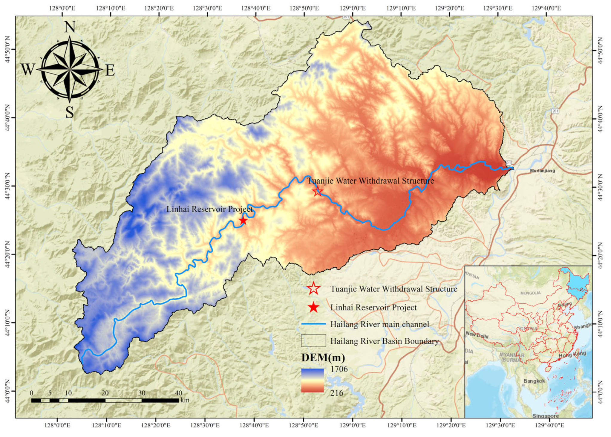
The Linhai Reservoir Project, the core research subject of this study, is located in Hailin City, which is under the administration of Mudanjiang City, Heilongjiang Province. The reservoir is situated in the middle and upper reaches of the Hailang River. As a China Standard Large (II) type reservoir, its primary purpose is water supply, supplemented by flood control, irrigation, and secondary power generation. The Hailang River, a typical mountainous river in the northeastern high-altitude cold region, flows into the Mudanjiang River downstream as a tributary. The reservoir controls a drainage area of 1562 km
2, accounting for 29.7% of the Hailang River Basin and 4.15% of the Mudanjiang River Basin. The United Front Water Diversion Complex, a component of the project, is located 3 km upstream of Changting Town on the middle reaches of the Hailang River and controls a drainage area of 2424 km
2 [
9]. The Linhai Reservoir provides a water supply for urban areas, agricultural irrigation, industry, and ecological environments. Therefore, research on operational scheduling strategies to ensure water supply security during the low-flow period of Linhai Reservoir is particularly important.
This research aims to develop a model for coordinated water supply-ecology operation of cold-region reservoirs, integrating Linhai Reservoir’s three-dimensional terrain data and dam project parameters. Using the cumulative anomaly method, the 65-year hydrological sequence was divided into six typical years, consistent with national standards, and the drought level classification was further refined. Coupling the HEC-RAS one- and two-dimensional hydrodynamic models with a dynamic regulation and release strategy, this study quantifies the synergistic effects of gate operation (opening/closing) and reservoir storage regulation on water level-discharge relationships. A dynamic water storage plan, driven by a flood-season flow threshold, is proposed to mitigate ice jam risk and enhance reservoir storage utilization efficiency. Simulating six scenarios ranging from peak-flow to extreme drought years, this study systematically evaluates the supply reliability, ecological compliance rate, and engineering risk under different operational strategies. This reveals the operational bottlenecks of cold-region reservoirs during extreme drought years and proposes multi-source integrated protection pathways. This study deeply integrates the specific characteristics of cold regions into multi-objective scheduling, providing a scientific basis for the regulation of Linhai Reservoir. Furthermore, this study offers a paradigm for resolving the conflict between ensuring water supply and protecting ecology in similar projects.
2. General Overview of the Study Area
The Linhai Reservoir Project in Mudanjiang City, Heilongjiang Province, is located within the jurisdiction of Hailin City, which is under the administration of Mudanjiang City. It is situated in the upper reaches of the Huali River. The geographical coordinates of the reservoir area are 128°36′49″ to 128°39′33″ east longitude and 44°24′06″ to 44°26′33″ north latitude. It is approximately 60 km away from the urban area of Hailin City and about 115 km away from Mudanjiang City. The control basin area above the dam site is 1562 km
2 [
10], accounting for 29.7% of the Huali River Basin and 4.15% of the Mudanjiang River Basin. The United Front Water Intake Structure, a supporting facility for the project, is located 3 km upstream of Changting Town on the middle reaches of the Hailang River, controlling a drainage area of 2424 km
2 [
11]. Mudanjiang City serves as the economic center of southeastern Heilongjiang Province. Hailin City, a county-level municipality within its jurisdiction, primarily cultivates rice and corn. Currently, the lack of reservoir regulation results in inadequate agricultural water supply security, while urban water supply heavily depends on excessive groundwater extraction. With population growth and industrial development in Mudanjiang City, water demand is projected to rise to 1.64 billion m
3/year. However, current water sources are insufficient to meet this demand, necessitating the urgent need for supplementary surface water from the Hailang River.
The Hailang River Basin exhibits topography with higher elevations in the west and lower elevations in the east, having an average elevation of 500 m [
12]. The upper reaches consist of foothills and low-lying areas along the Zhangguangcai Ridge, dominated by forest vegetation. Downstream, the river course gradually widens, forming an alluvial plain. (Sentence is concise and clear; no major edits are needed.) The Linhai Reservoir dam site is located in a narrow valley section where the main river channel is “U”-shaped, approximately 70 m wide, with a gradient of 3%. The United Front Structure section features a straighter river channel, 80 m wide, and a gradient of 2%, exhibiting typical characteristics of mountainous rivers. Hydrologically and meteorologically, the Hailang River Basin falls under the temperate monsoon climate zone. The basin has an average annual temperature of 3 °C, with extremes of 35.8 °C and −38.8 °C. Average annual precipitation is 1110 mm in the upper reaches and 530 mm in the lower reaches, with July and August accounting for 51% of the total annual precipitation. The average annual surface water evaporation is 603 mm, and the maximum permafrost depth reaches 2 m. The Hailang River’s runoff is primarily derived from precipitation. The natural runoff within the basin is unevenly distributed throughout the year. During the dry season (November to the following April), the supply and demand situation is extremely tense, with the runoff accounting for less than 20%, and the minimum monthly flow is only 0.32 m
3/s (
p = 95%). The river is frozen for 150 days (from November to mid-April), with an ice thickness of 1.0–1.76 m, and the spring snowmelt flow accounts for approximately 15%.
Linhai Reservoir (Class II large, Chinese standard) has a normal pool level of 492 m and a storage capacity of 1.76 billion m
3 [
13]. Linhai Reservoir is integrated with the United Front Withdrawal Structure under a supply system prioritizing reservoir interval water over reservoir replenishment. Linhai Reservoir supplies 1.79 billion m
3 annually (projected for 2035) to meet Mudanjiang City’s urban water demand (95% assurance) and irrigate 154,000 mu of farmland. During low-flow periods, the reservoir releases an ecological base flow of 1.52 billion m
3 annually (on average) to maintain downstream channel ecology.
In conclusion, the research on the scheduling strategy for ensuring water supply security during the dry season of Linhai Reservoir is of particular significance. This study focuses on the optimization of water resource allocation during the dry season, which is of great significance for alleviating regional water shortages and maintaining the health of rivers. It also provides a certain scientific reference basis for the multi-objective coordinated operation of reservoirs in the same type of high-latitude cold regions; the locations of the Hailang River Basin, Linhai Reservoir, and Tuanjie Water Diversion Hub Project are shown in
Figure 1.
3. Introduction to Research Methods and Data Processing
3.1. Data Sources
This study employs HEC-RAS software to develop 1D and 2D hydrodynamic models for the Linhai–Tuanjie section of the Hailang River Basin. The models simulate the hydrodynamic effects resulting from the partially completed Linhai Reservoir Project, the Tuanjie Water Withdrawal Structure Project, and the Linhai Reservoir water conveyance pipeline. Specifically, the simulations investigate the impacts of these developments on downstream conditions, encompassing hydrology, river channel evolution, and the construction of hydraulic structures. The study assesses the implications of these impacts on urban water supply for Hailin and Mudanjiang, farmland irrigation for surrounding townships, and the fulfillment of ecological flow requirements throughout the basin. The objective of this study is to provide scientific recommendations for optimizing water resource allocation during low-flow periods, alleviating water shortages, and ensuring the ecological function of the downstream river channel.
Based on this, the study requires the following data: basin topographic data, continuous time series river flow data, hydraulic structure parameters, basin soil type data, and water demand data for downstream cities and towns.
The basin topographic data were obtained from the ASTER GDEM 30 m resolution digital elevation model (DEM), provided by the Chinese Academy of Sciences Environmental Data Center. Version 10.8 of ArcGIS software was used for subsequent processing. The continuous time series of river flow data for the basin was derived from measured hydrological records at the Changtingzi Hydrological Station, including daily flow, water level, and ice conditions. The hydraulic structure parameters were obtained from the ‘Feasibility Study Report for the Linhai Reservoir Project in Mudanjiang City, Heilongjiang Province’ (Heilongjiang Water Conservancy and Hydropower Survey and Design Research Institute). The underlying surface data comprised soil type data and land use data. The soil type data were sourced from the “China 1:100 Million Soil Type Dataset” (v4.0), provided by the Institute of Soil Science, Chinese Academy of Sciences (Nanjing). ArcGIS software was used to extract and process this data for the Hailang River Basin. The land use data were obtained from the ‘National 30 m Resolution Land Cover Fine Classification Product for 2020’ (National Earth System Science Data Center). ArcGIS software was used to extract and process this data for the Hailang River Basin. The predicted water demand data for downstream cities and towns was obtained from the ‘Urban and Rural Water Supply Planning Report for Mudanjiang and Hailin Cities,’ prepared by the HIT. The findings of this report were subsequently confirmed by the Mudanjiang City government.
3.2. Research Methodology
3.2.1. Typical Year Classification
This study focuses on the water supply guarantee issue of Linhai Reservoir during the dry season. Through the HEC-RAS software, simulations were conducted. Historical runoff data of the Hailang River Basin, where Linhai Reservoir is located, were coupled in the software. According to the “GB/T 50095-2014 Standard for Basic Terminology and Symbols of Hydrology” [
14], the historical runoff series was divided into different typical years by frequency using the empirical frequency method.
The empirical frequency method establishes an empirical relationship between observed values and their occurrence frequencies by utilizing ranking statistics derived from a historical hydrological sequence. This method is distribution-free, as it does not require assumptions regarding the data distribution type; it directly calculates the empirical cumulative probability for each magnitude level based on historical data. The detailed calculation formulas are as follows: The detailed calculation formulas are presented below:
In the formula, represents the empirical frequency of the m-th sample, is the serial number after descending ranking, and is the sample quantity.
The cumulative anomaly method is a non-linear statistical method that visually determines the trend of changes in discrete data points using a curve [
15]. Anomaly definition: In a group of climate variables (
,…,
), the deviation of a particular value
from the average (
) of the group’s data, which is
. The cumulative anomaly refers to the time
corresponding to a climate variable
; it is the sum of all anomalies up to the time
. The value obtained from adding these together is the cumulative anomaly [
16]. The formula is as follows:
In the formula,
represents the observed value at the t-th time point,
represents the mean of the series, and
represents the cumulative anomaly value at the i-th time point. By plotting the cumulative anomaly corresponding to each time point, a cumulative anomaly curve is drawn. The upward or downward trend of the curve indicates the increase or decrease in the anomaly values. From the ups and downs of the curve, the long-term significant evolution trend and persistent changes can be judged, and even the time of occurrence of a mutation can be determined [
17].
3.2.2. Model Validation
Reliable hydrological data (such as flow rate, water level, etc.) are the foundation for constructing reservoir operation models and formulating water supply assurance strategies. This study comprehensively evaluates the error characteristics of the simulated hydrological data compared to the observed data using the following indicators to ensure the reliability of the simulation:
Correlation Coefficient (CC): Measures the strength and direction of the linear relationship between simulated and observed values;
Kling–Gupta Efficiency Coefficient (KGE): Comprehensively evaluates the model’s performance based on linear correlation, variance ratio, and hydrological bias (water balance). Values closer to 1 indicate better performance.
Relative Bias (
RB): Quantifies the systematic overestimation (RB > 0) or underestimation (RB < 0) of the simulated values [
18].
Nash Efficiency Coefficient (NSE): Evaluates the overall goodness of fit of the model; range is (−∞1).
Coefficient of Determination (R2): Explains the proportion of the variance in the observed data that is explained by the model (range 0 to 1).
Mean Absolute Error (
MAE) [
19]: Directly reflects the average absolute deviation between simulated values and observed values.
Root Mean Square Error (
RMSE): Highlights the impact of extreme errors. The detailed calculation formulas for each coefficient are as follows:
In the formula, and are the simulated and observed values of runoff data, respectively. and are the means of the observed and simulated values, respectively. and are the standard deviations and expected values of the simulated and observed values, respectively. is the sample size.
3.2.3. HEC-RAS Model
Based on the previous introduction, the HEC-RAS system has a graphical user interface, hydraulic analysis subroutines (constant flow and non-constant flow subroutines), data storage and management, chart creation and data summarization functions, and can perform one-dimensional constant flow and one-dimensional or two-dimensional non-constant flow hydraulic calculations. Its basic functions include the following four aspects: (1) Steady-flow water surface computations; (2) One-dimensional (1D) and two-dimensional (2D) unsteady-flow simulations; (3) Sediment transport calculations, including variable boundary conditions (cohesive and non-cohesive bed materials); (4) Water temperature and quality transport modeling. These capabilities align with the functionalities offered by the HEC-RAS system, which include steady-flow water surface computations, 1D and 2D unsteady-flow simulations, sediment transport calculations with variable boundaries (cohesive and non-cohesive bed materials), and water temperature and quality transport modeling. It supports one-dimensional steady-flow calculations and one- or two-dimensional unsteady-flow hydraulic analyses. Using these capabilities, HEC-RAS can simulate the effects of hydraulic structures, such as bridges, spillways, weirs, gates, and detention basins, on water flow. It can also perform 2D flood propagation numerical simulations [
20,
21,
22,
23,
24,
25,
26,
27,
28].
In the equation, represents time; and are the components of velocity in the and directions, respectively; is the height relative to the undisturbed water surface; is the static water depth; is the total water depth, where (); is the water density, and is the reference water density; is the Coriolis parameter, defined as (), where () is the Earth’s angular velocity and () is the latitude; and are accelerations caused by the Earth’s rotation; , , and are horizontal viscous stresses; is the source/sink term, where positive values indicate sources and negative values indicate sinks; and are the components of the source/sink velocity in the and directions, respectively.
3.3. Data Processing
3.3.1. Typical Year Division
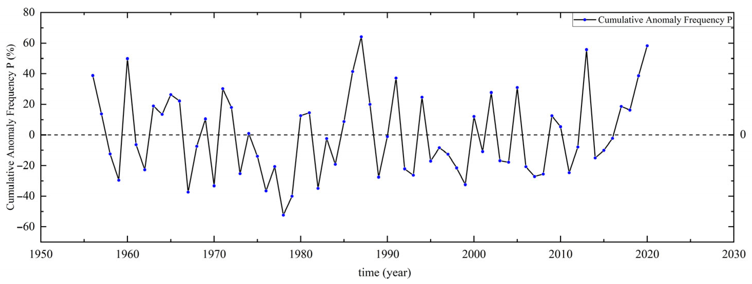
This study combined the empirical frequency method and the cumulative anomaly method to classify the Haihe River Basin’s annual total water volume for the 1956–2020 period into six typical year types. Frequency anomalies and total water volume ranges for these types are presented in
Table 1, while the cumulative anomaly frequency is shown in
Figure 2.
Using the empirical frequency method and the cumulative anomaly method, it was determined that the Hailang River Basin experienced consecutive years of abundant water (2019–2020), consecutive years of normal water (2017–2018), consecutive years of mild drought (2014–2015), consecutive years of moderate drought (2006–2007), consecutive years of severe drought (1976–1977), and consecutive years of extreme drought (1978–1979). Studies on water supply during low-flow periods in the Hailang River Basin and similar northeastern cold-region rivers suggest significant interannual continuity in hydrological cycles. According to the ‘Standard for Basic Hydrological Terms and Symbols (GB/T 50095-2014)’, hydrological year definitions should reflect the completeness of the basin’s water cycle. The Hailang River Basin (study area) experiences most of its annual runoff (65%) during the June–September rainy season. The subsequent May spring flood typically marks the end of this cycle. A hydrological year defined from June to the following May comprehensively covers the precipitation-storage-melting process and avoids the artificial separation of wet and dry periods inherent in calendar years. Therefore, this study adopts this definition, using a hydrological year spanning June to the following May. Data for the following categories of years were selected from the respective hydrological years: flood years (2019 hydrological year, June 2019–May 2020); normal water years (2017 hydrological year, June 2017–May 2018); mild drought years (2014 hydrological year, June 2014–May 2015); moderate drought years (2006 hydrological year, June 2006–May 2007); severe drought years (1976 hydrological year, June 1976–May 1977); and extreme drought years (1978 hydrological year, June 1978–May 1979).
3.3.2. Model Accuracy Verification Results
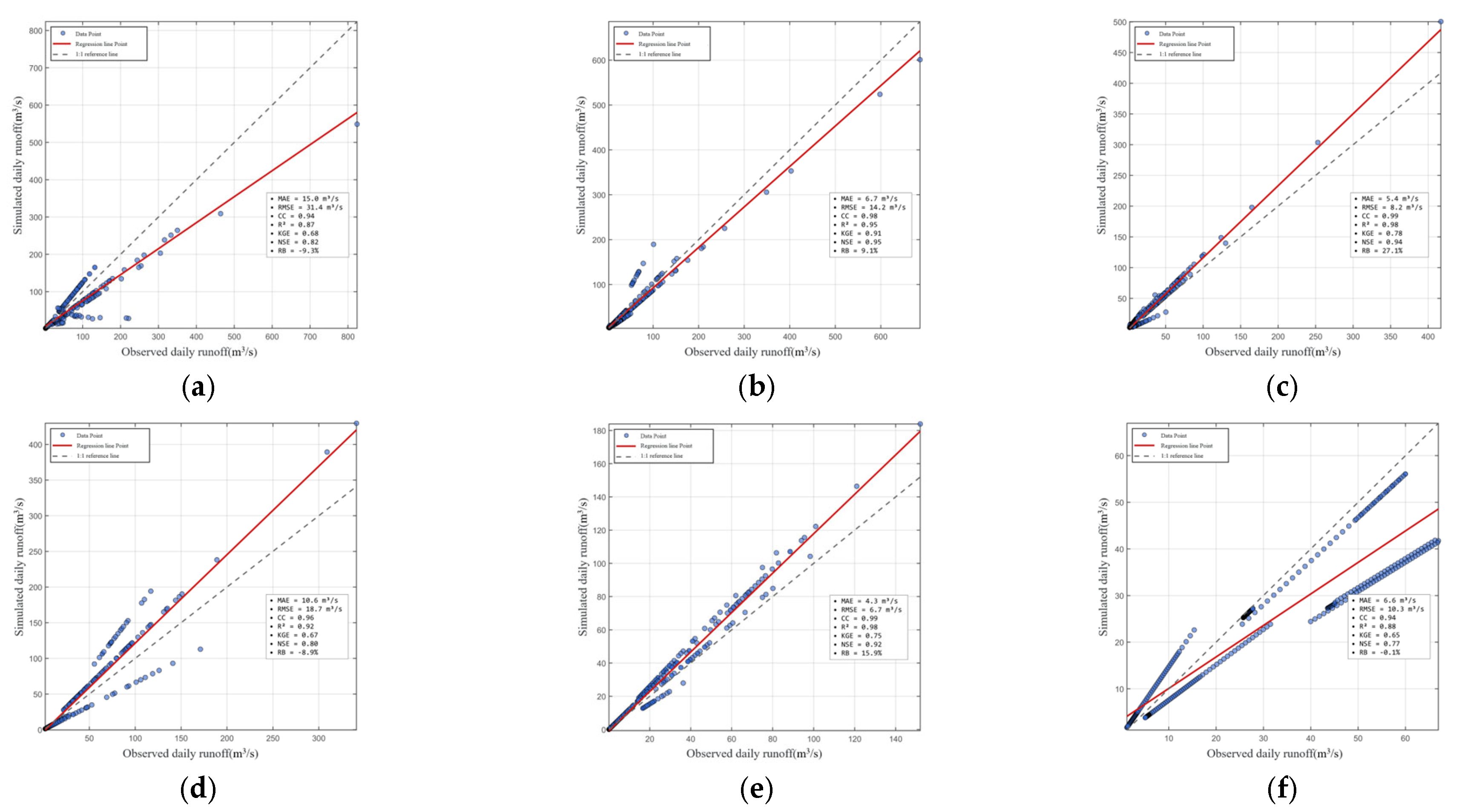
This study verified the reliability of the HEC-RAS model using multidimensional indicators to ensure the scientific validity of the low-flow water supply simulation. Simulations of river flow for six different typical years were conducted using the HEC-RAS two-dimensional hydrodynamic model, excluding Linhai Reservoir and Tuanjie Dam from the model setup. Based on daily measured data from the Changtingzi Hydrological Station (1956–2020), six typical years representing abundant, normal, mild drought, moderate drought, severe drought, and extreme drought conditions were selected for parameter calibration and validation. The results show that the model’s correlation coefficient (CC) ranged from 0.94 to 0.99, and the Kling-Gupta efficiency coefficient (KGE) ranged from 0.65 to 0.91, indicating a high degree of fit between simulated and observed flow hydrographs. The relative bias (RB) remained within ±5%, and the Nash efficiency coefficient (NSE) ranged from 0.80 to 0.95, indicating that the model’s systematic errors are controllable. Details of these model verification coefficients are presented in
Table 2 and
Figure 3a–f. Multi-indicator validation confirms the model’s high-precision capabilities in simulating the hydraulic response of alpine reservoirs and the coupling effects of ice conditions, thereby providing a reliable foundation for developing water supply security strategies.
3.3.3. HEC-RAS Model Simulation
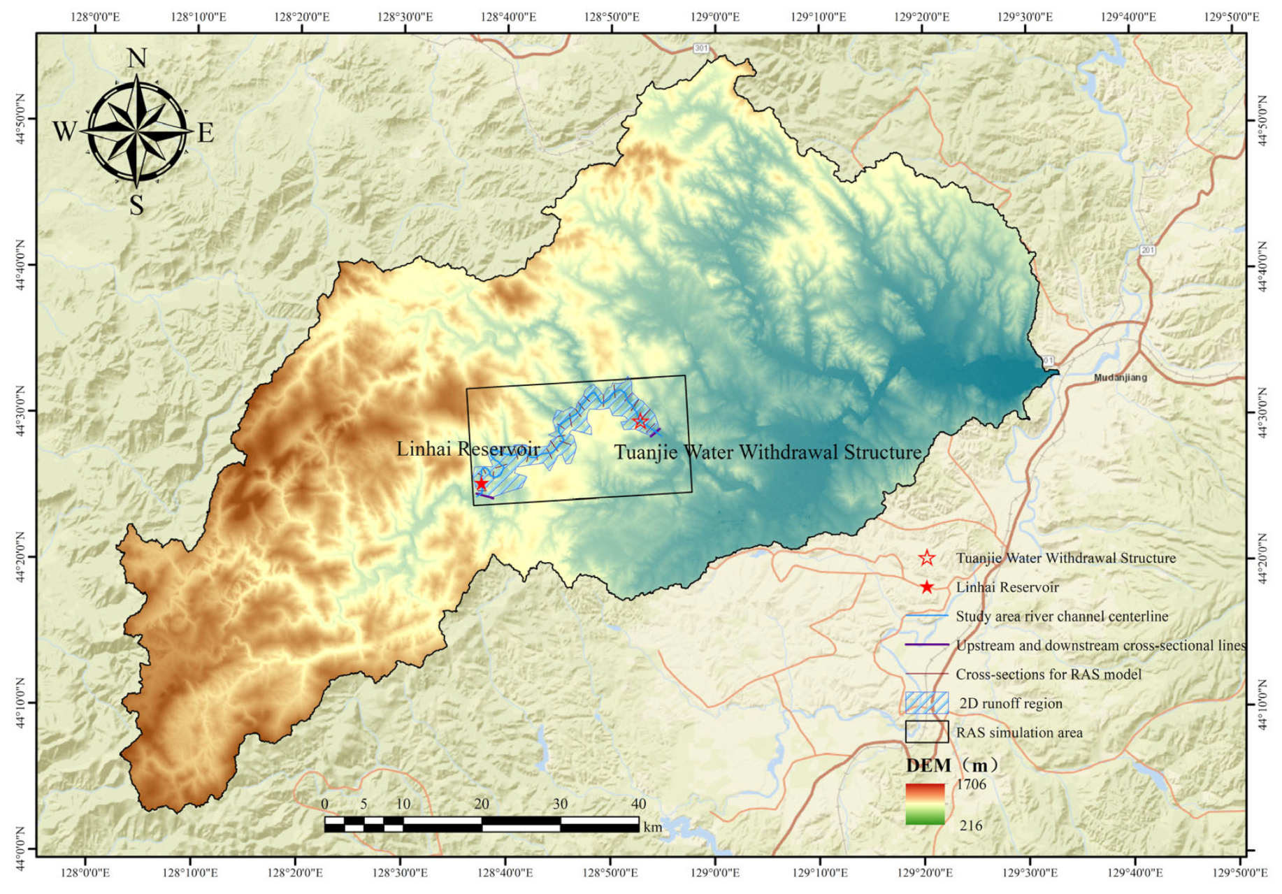
This study constructed a two-dimensional hydrodynamic model for the “Linhai-Tuanjie” reach using HEC-RAS and conducted unsteady flow numerical simulations. Recognizing that the basin has no major tributaries, the main channel of the Halang River and the surrounding shoals from the Linhai Reservoir to the Tuanjie Water Intake Structure were defined as the two-dimensional flow area. To ensure the accuracy of the model simulation, a structured grid with a size of 30 m × 30 m was adopted for discretization, generating approximately 104,689 calculation units, thereby achieving a refined representation of the terrain’s minor fluctuations. The SA/2DConnection module was used to incorporate the gravity dams of the Linhai Reservoir and the Tuanjie Water Intake Structure, along with other hydraulic structures, into the model. Gate opening and closing thresholds were set, and the model was coupled with upstream runoff series from 1956 to 2020. Based on the RAS Mapper, a one-dimensional cross-section projection is generated. According to the data, the freezing period at the Hailang River Changtingzi monitoring station typically lasts from early November to mid-April of the following year, with an average freezing duration of approximately 160 days, an average ice thickness of 1.0 m, and a maximum ice thickness of 1.76 m. By importing the ice cover data into the one-dimensional model, the impact of the ice cover on reservoir operation during and after the freezing period can be accurately simulated. Following model validation, the Nash efficiency coefficient (NSE) ranged from 0.80 to 0.95, and the Kling–Gupta efficiency coefficient (KGE) ranged from 0.65 to 0.91. The model can accurately simulate water surface elevations during low-flow periods and flow fluctuations, providing a reliable numerical experimental platform for multi-scenario operation. The geographical spatial data for the study area were calibrated using the WGS-1984 coordinate system. Terrain rendering and spatial matching of cross-sections were performed via GIS construction (as shown in
Figure 4), ensuring topological consistency between the model boundaries and the measured terrain.
4. HEC-RAS Calculation Results
By utilizing HEC-RAS software to establish a joint scheduling model for the “Linhai-Tuanjie” system and coupling it with different typical annual runoff sequences, this study simulates and analyzes the downstream withdrawal section’s runoff flow rate after the reservoir’s construction. It details the guarantee rates for urban and rural water supply as well as the compliance rates for ecological base flow under various typical conditions through reservoir operations. The simulation results indicate that through reservoir regulation and storage, the annual water supply guarantee rate and ecological compliance rate both reach 100% during flood years, demonstrating effective provision for both water supply and ecological requirements. In normal years, the annual water supply guarantee rate is 97.3%, and the ecological compliance rate is 95.6%. In mild drought years, the annual water supply guarantee rate is 93.5%, with an ecological compliance rate of 91%. In moderate drought years, the annual water supply guarantee rate is 89%, while the ecological compliance rate is 76%. In severe drought years, the annual water supply guarantee rate drops to 72.8%, and the ecological compliance rate is 67%. In extreme drought years, the annual water supply guarantee rate is 58.3%, with an ecological compliance rate of 41%. An overview of the water supply and ecological compliance rates across six different hydrological years is provided in
Table 3, with further details of the model simulation presented below.
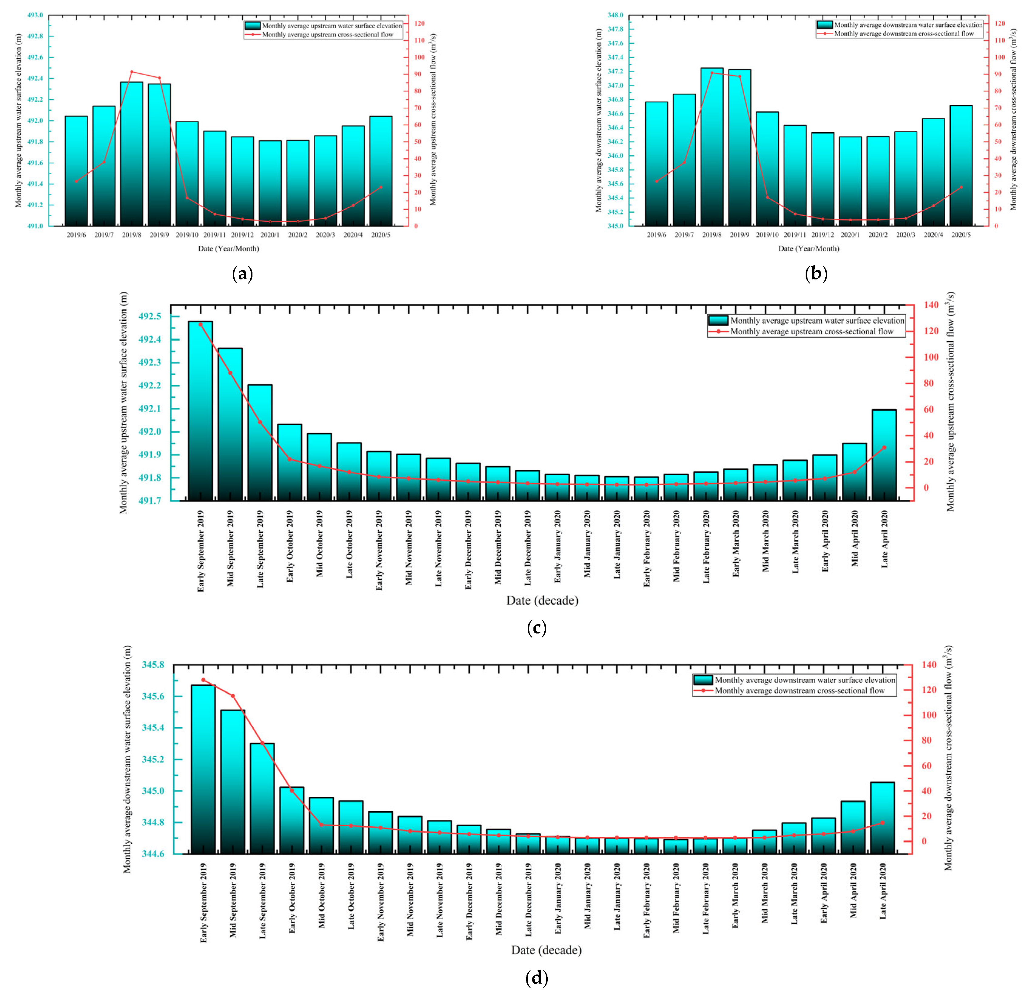
4.1. Flood Year
During flood years, the reservoir’s inflow significantly exceeds the long-term average. The annual runoff exhibits a “bimodal” characteristic (
Figure 5a,b). The peak inflow during the main flood season (June–August) reaches 78.3 m
3/s, while the reservoir maintains a water level fluctuation amplitude of ≤0.15 m through dynamic flood releases. From September to October (end of flood season), inflow rates dropped to 18.7–23.5 m
3/s, the storage rate reached 97.3%, and the water level increased from 491.8 m to 492.0 m (
Figure 5c,d). During the frozen period (November to early April of the following year), inflow rates plummeted sharply to 4.2–6.8 m
3/s. However, thanks to water stored during the previous high-flow period, outflow rates remained stable at 8.1–9.6 m
3/s, comfortably exceeding the ecological threshold of 3.5 m
3/s and meeting urban water demand of 120,000 m
3/day. During the thawing period (mid-April), spring floods combined with snowmelt runoff caused inflow rates to increase to 15.3 m
3/s. Water levels subsequently rose back to 491.6 m. Model results indicated that both the annual water supply guarantee rate and ecological compliance rate reached 100%, demonstrating excellent performance in ensuring a stable water supply while maintaining ecological standards throughout the year.
During the freezing period (November–mid-December), the reservoir’s inflow rate decreased from an average of 6.8 m
3/s in November to 4.2 m
3/s by mid-December (see
Figure 5c). Concurrently, water stored at the end of the flood season helped maintain a high water level between 491.5 and 492.0 m. The outflow rate remained stable at 8.1 to 9.6 m
3/s, significantly exceeding the ecological threshold by 131–174%. The reservoir capacity curve showed a linear decline, resulting in an average daily water supply of 123,000 m
3—2.5% above the design requirement. Ice thickness increased from 0.2 to 0.8 m, keeping the risk of ice jams below 5%. During the freezing period (November–mid-December), the reservoir’s inflow rate decreased from an average of 6.8 m
3/s in November to 4.2 m
3/s by mid-December (see
Figure 5c). Concurrently, water stored at the end of the flood season helped maintain a high water level between 491.5 and 492.0 m. The outflow rate remained stable at 8.1 to 9.6 m
3/s, significantly exceeding the ecological threshold by 131–174%. The reservoir capacity curve showed a linear decline, resulting in an average daily water supply of 123,000 m
3—2.5% above the design requirement. Ice thickness increased from 0.2 to 0.8 m, keeping the risk of ice jams below 5%.
During the later phase of the freezing period (late December–February), the average inflow rate dropped to 4.5 m
3/s (see
Figure 5c). To manage water supply, the reservoir adopted a “supply priority” approach, relying on stored water. This caused the water level to fall from 491.2 to 490.5 m, releasing 0.12 million m
3. The outflow rate remained stable at 8.0 ± 0.3 m
3/s, achieving an ecological compliance rate of 98.7% and a water supply guarantee rate of 100%. Ice thickness increased to 1.2 m; the hydraulic gradient deviation, at 6.7%, fell within a reasonable error range (see
Figure 5d).
During the thawing period (March–mid-April), the inflow rate rose to 15.3 m
3/s, largely driven by snowmelt, which accounted for 62% of the increase. The water level recovered to 491.6 m within 30 days, demonstrating an average daily rise of 0.02 m. The outflow rate was dynamically adjusted to between 9.6 and 12.4 m
3/s. Concurrently, the cross-sectional flow velocity increased from 0.35 m/s to 0.68 m/s (see
Figure 5d).
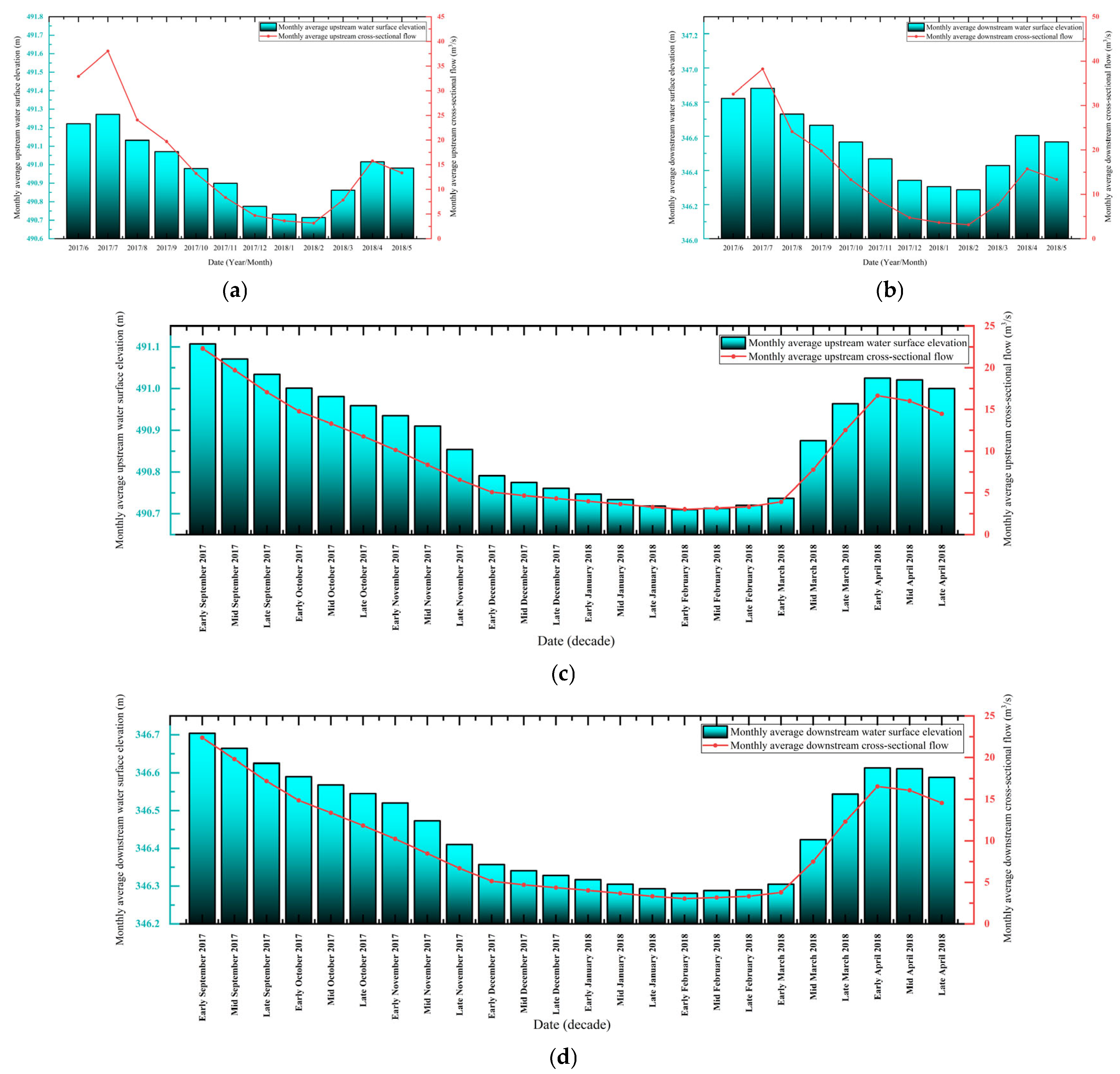
4.2. Normal Water Year
In an average water year, the inflow rate approximates the long-term average; however, supply-demand mismatches are evident during the ice-covered period (see
Figure 6a,b). The peak flow rate during the main flood season reached 42.6 m
3/s, utilizing 92% storage capacity. During the ice-covered period, the average inflow rate was 3.8 m
3/s. Concurrently, the water level dropped from 492.0 to 489.2 m, representing 83% of the flood control limit. The outflow rate was maintained between 5.2 and 7.8 m
3/s, achieving an ecological compliance rate of 95.6%. Water supply shortfalls are addressed through coordinated management among reservoir areas (see
Figure 6c,d). The annual water supply guarantee rate is 97.3%, and the ice jam risk probability is 12%. Given this risk, the thermal ice-melting system is activated.
During the freezing period (November–mid-December), the average inflow rate decreased to 5.3 m
3/s, representing a 22% reduction compared to wet-year averages. The reservoir adopted a “staggered storage and release” strategy. Consequently, the water level dropped from 492.0 m to 490.8 m, while the outflow rate was maintained between 6.5 and 7.8 m
3/s, achieving 100% ecological compliance. However, a three-day water supply shortfall occurred in early December, with an average daily deficit of 114,000 m
3. The slope of the reservoir capacity curve increased by 15% (see
Figure 6c), indicating weakened regulation capability.
During the later freezing period (late December–February), the average inflow rate was 3.8 m
3/s, and the water level decreased linearly to 489.2 m. The outflow rate ranged from 5.2 to 5.8 m
3/s, utilizing 0.02 billion m
3 of dead storage capacity (located below the 472 m elevation). The water supply guarantee rate was 97.3%. On days when standards were not met, a supplementary water supply of 12,000 m
3/d was provided via the Unity Hub (see
Figure 6d).
During the thawing period (March–mid-April), the inflow rate recovered to 12.7 m
3/s, with snowmelt contributing 55%. The water level rose by 2.1 m within 30 days, reaching a peak outflow rate of 10.8 m
3/s. On 37% of days, the flow velocity in the water transmission pipeline exceeded 2 m/s, necessitating the activation of pressure regulation valves for control (see
Figure 6d).
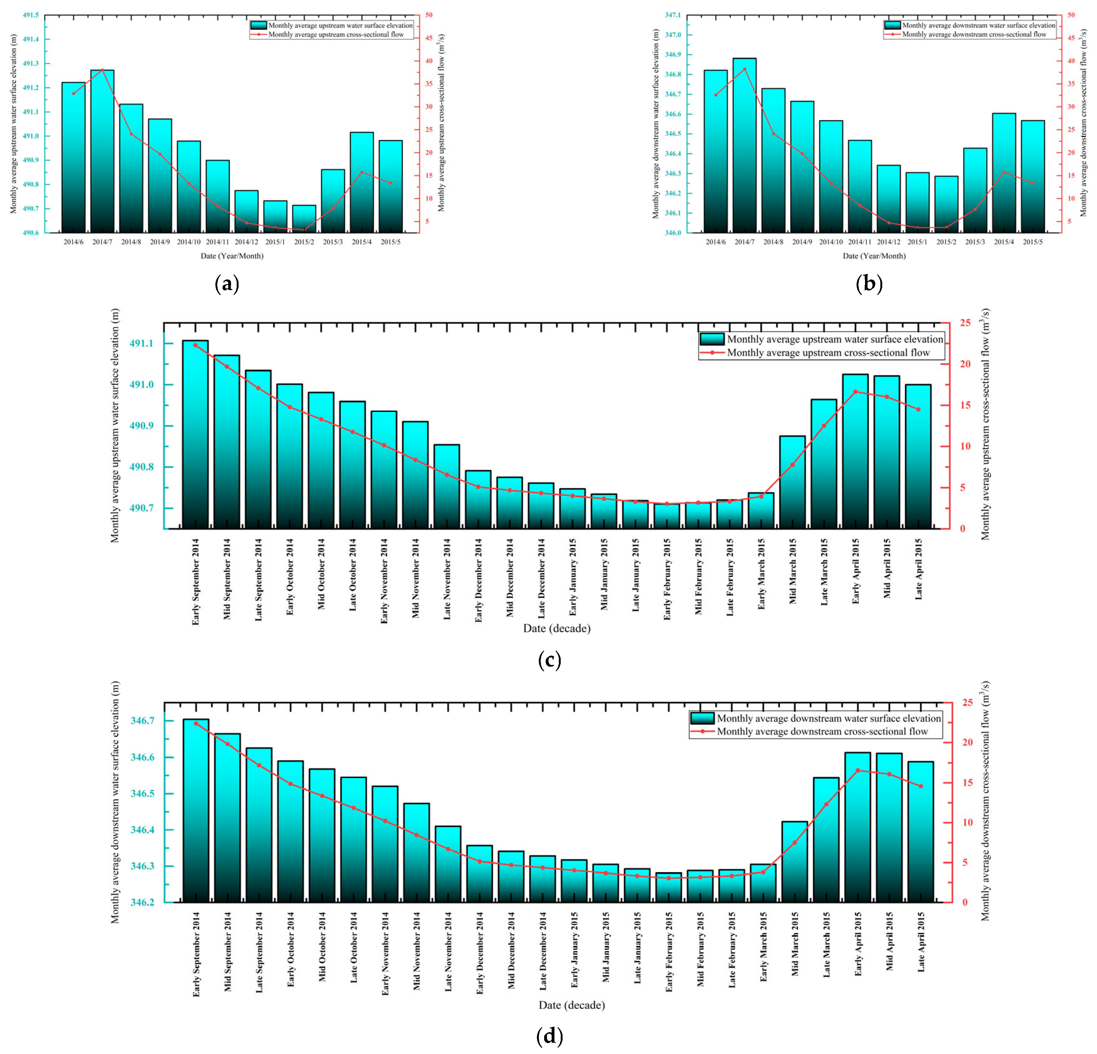
4.3. Mild Drought Year
During a mild drought year, inflow rates decrease by 15% compared to average conditions. This results in heightened supply and demand pressure during the freezing period (see
Figure 7a,b). During the main flood season, the peak flow rate reaches 38.4 m
3/s, while the water storage rate is maintained at 85%. During the freezing period, the average inflow rate is 3.2 m
3/s. Concurrently, the water level decreases from 492.0 m to 483.5 m. The outflow rate ranges from 4.5 to 5.2 m
3/s, achieving an ecological compliance rate of 91%. Seasonal water transfers were utilized to supplement the water supply shortfall (see
Figure 7c,d), resulting in an overall water supply guarantee rate of 93.5% for the year.
During the freezing period (November to mid-December), the average inflow rate is 4.1 m
3/s, while the water level gradually decreases from 492.0 m to 488.7 m, The outflow rate ranges from 5.0 to 5.5 m
3/s, achieving an ecological compliance rate of 94%. Compared to an average water year, the reservoir release rate increases by 20% during this period (see
Figure 7c), reflecting heightened regulation pressure.
During the frozen period (late December to February), the average inflow rate decreases to 2.9 m
3/s, and the water level drops to 483.5 m. The outflow rate varies from 4.5 to 4.8 m
3/s. Concurrently, 0.05 billion m
3 of dead storage capacity is utilized, and the ice thickness reaches 1.6 m. The water supply guarantee rate is 92%. On non-compliance days, an additional 18,000 m
3/d is supplied (see
Figure 7d). During the thawing period (March to mid-April), the inflow rate rebounds to 10.5 m
3/s, of which 50% is attributed to snowmelt. The water level subsequently recovers to 487.2 m. The peak outflow rate reaches 9.2 m
3/s. The flow velocity at the cross-section is 0.58 m/s (see
Figure 7d), deviating by 8.3% from the natural river channel.
Furthermore, pipeline overloads occurred on 25% of days during this period, indicating the need to optimize scheduling strategies.
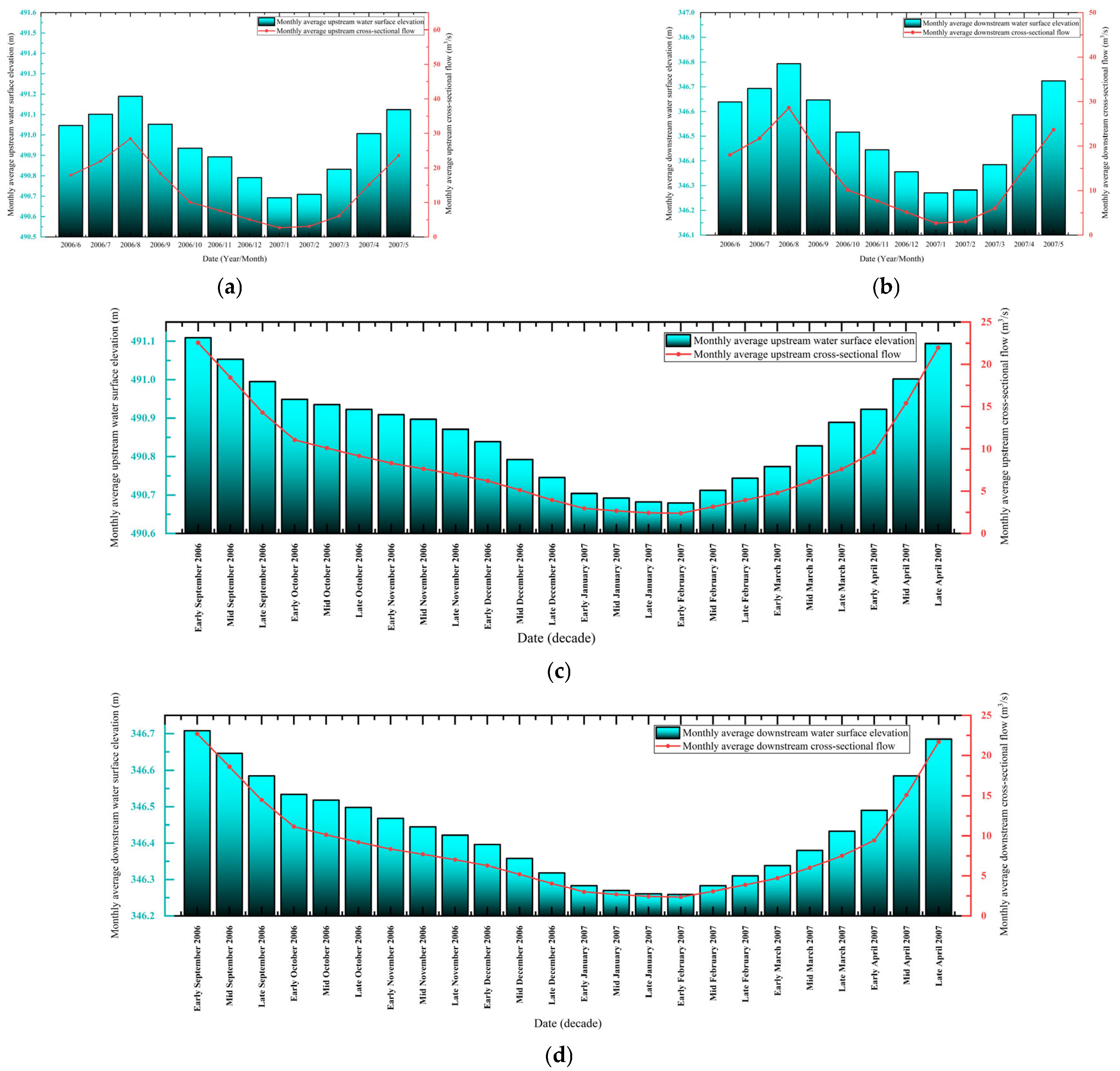
4.4. Moderate Drought Year
During a moderate drought year, inflow rates decrease by 35% compared to average conditions. The average inflow rate during this period (November to the following April) is 3.2 m3/s. The water level at Shuhai Reservoir upstream gradually dropped from the normal storage level of 492 m in November to a minimum of 478 m in February, close to the dead water level of 472 m. This represents a total decline of 14 m, with an average monthly drop of 2.8 m. Downstream at Changtingzi Hydrological Station, the water level, significantly influenced by reservoir regulation, maintained a range of 2.1 to 2.4 m from November to December. This level represents an elevation of 0.6 to 0.9 m compared to natural conditions. However, from January to February, due to reservoir releases, the water level fell back to a range of 1.6 to 1.8 m. The ecological flow compliance rate was 89%, with non-compliance periods concentrated between late January and early February. To maintain a minimum outflow of 3.5 m3/s, dead storage capacity below the elevation of 472 m (0.18 billion m3) was utilized.
During the freezing period (November to mid-December), the inflow rate decreased stepwise from 4.8 to 2.9 m
3/s (see
Figure 8c). Concurrently, the water level fell from 492.0 to 485.3 m at an average daily rate of 0.15 m. The outflow rate was dynamically regulated between 4.5 and 5.1 m
3/s, exceeding the ecological threshold by 28–45%. A total of 0.28 billion m
3 of reservoir capacity was released, and the flow rate in the water conveyance pipelines was reduced to 1.2 m/s.
During the frozen period (late December to February), the average inflow rate further declined to 2.1 m
3/s (see
Figure 8c). The water level continued to decrease at an accelerated rate, reaching 478.2 m (with an average daily drop of 0.18 m). Outflow rates ranged from 4.1 to 4.3 m
3/s. A significant drop occurred between 16 and 22 January, during which the outflow fell below 3.8 m
3/s for seven consecutive days, reaching a minimum of 3.52 m
3/s. This triggered the utilization of dead storage capacity, drawing from the storage volume below the elevation of 472 m (0.18 billion m
3). The ice thickness reached 1.8 m, and the peak operational force on the gate was 920 kN (design value: 1000 kN).
During the thawing period (March to mid-April), the inflow rate increased to 8.7 m
3/s (with snowmelt contributing 58%), and the water level rebounded to 483.1 m within 30 days (see
Figure 8d). The outflow rate was adjusted to between 7.2 and 8.9 m
3/s, achieving a peak shaving rate of 12% during the spring flood. The average flow velocity at the cross-section increased from 0.28 to 0.61 m/s, and the deviation from the natural river channel expanded to 12% (see
Figure 8d), indicating the ongoing impact of reservoir capacity regulation on hydrodynamic conditions.
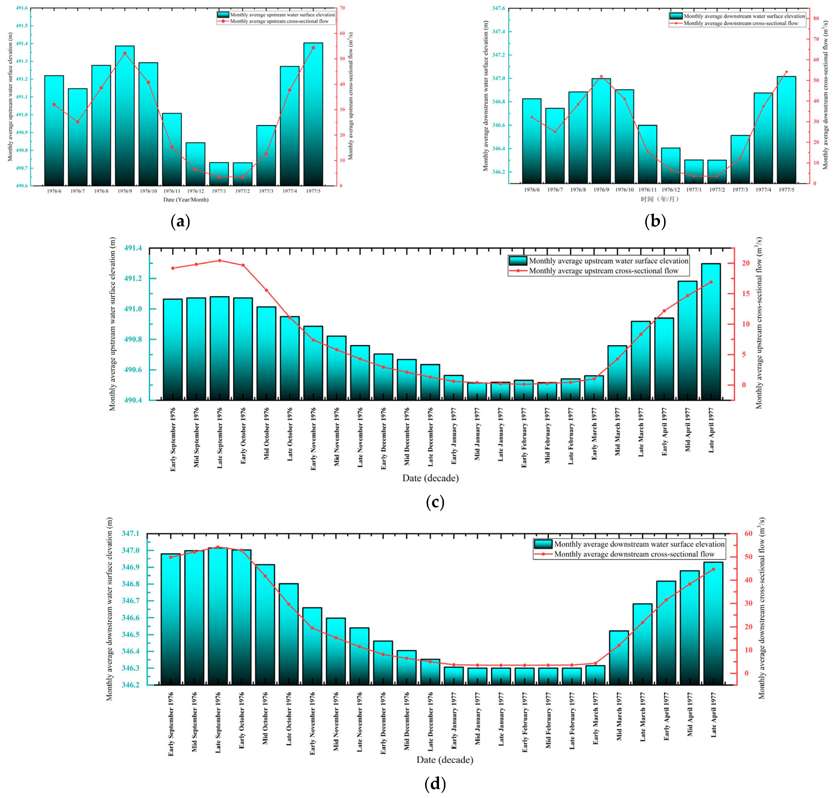
4.5. Severe Drought Year
In a severe drought year, the inflow rate sharply decreases to just 38% of the historical average, and runoff characteristics exhibit a “single peak early recession” pattern (see
Figure 9a,b). The peak flow during the main flood season is 25.4 m
3/s, representing a 40% reduction compared to an average water year. Furthermore, the storage rate is only 62%. During the ice-bound period, the average inflow rate is 1.8 m
3/s. By the end of December, the water level reaches the dead water level of 472 m (see
Figure 9c). The outflow rate ranges from 3.1 to 3.7 m
3/s, achieving an ecological compliance rate of 67%. To address the low flow conditions, the emergency backup water source mechanism must be activated. The overall water supply guarantee rate for the year is 72.8%. Concurrently, the risk of ice blockages reaches a probability of 35%.
During the freezing period (November to mid-December), the inflow rate sharply decreased from 3.2 to 1.5 m
3/s (see
Figure 9c). Concurrently, the water level declined at an average rate of 0.28 m per day, reaching the dead water level of 472 m. The outflow rate was maintained between 3.5 and 3.8 m
3/s, barely meeting the ecological flow requirement. Reservoir regulation capability was completely lost during this period. Water extraction from pipelines decreased to 98,000 m
3/day, representing 81.7% of the design demand, prompting the activation of emergency groundwater supplementation.
During the freezing period (late December to February), the inflow rate consistently remained below 1.2 m
3/s (see
Figure 9c). The release rate from dead storage during this period reached 0.01 billion m
3/month. The outflow rate ranged from 3.1 to 3.3 m
3/s. A significant drop occurred from 8 January to 14 February, during which the outflow remained below 3.5 m
3/s for 38 consecutive days, reaching a minimum of 2.9 m
3/s. Concurrently, ice thickness exceeded 2.0 m, increasing the risk of gate operational failure and necessitating mechanical icebreaking to maintain minimum flow capability.
During the thawing period (March–mid-April), the inflow rate rose to 6.4 m
3/s, with snowmelt contributing 73% to this increase. However, the available dead storage limited the rate of water level recovery to an average daily increase of only 0.08 m. The outflow rate was adjusted to between 5.7 and 6.8 m
3/s. The flow velocity at the cross-section reached 0.53 m/s (see
Figure 9d), which lagged 19% behind natural conditions.
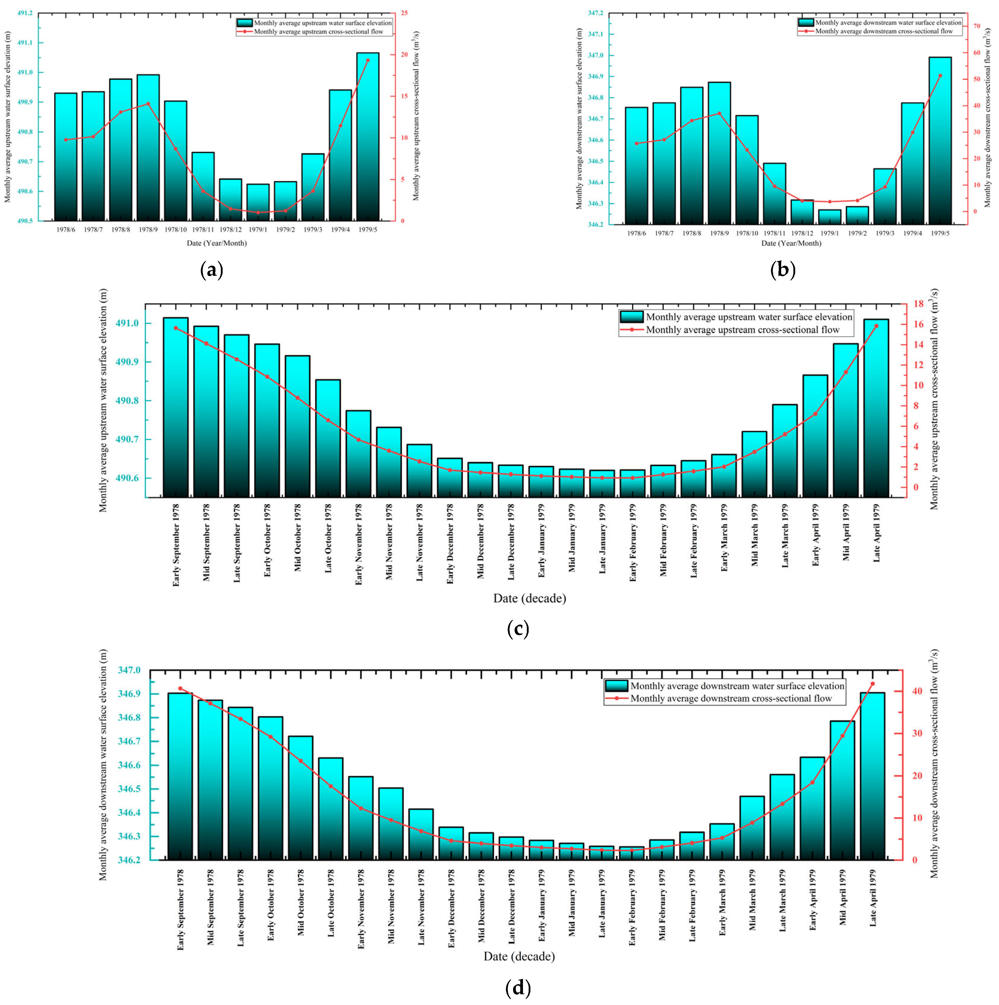
4.6. Extreme Drought Year
During the extreme drought year, the inflow rate was only 28% of the historical average, exhibiting a “no peak continuous drought” characteristic (see
Figure 10a,b). During the main flood season, the peak flow reached 18.9 m
3/s, representing a 55% decrease compared to an average water year. Concurrently, the storage rate was insufficient, remaining below 50%. During the ice-bound period, the average inflow rate dropped to 0.9 m
3/s. By mid-November, the water level reached the dead water level (see
Figure 10c). The outflow rate fluctuated between 2.6 and 3.2 m
3/s, achieving an ecological compliance rate of only 41%. The system entered a state of extreme regulation, with the overall water supply guarantee rate for the year reaching only 58.3%.
During the freezing period (November to mid-December), the inflow rate plummeted from 1.8 to 0.7 m
3/s (see
Figure 10c), causing the water level to drop dramatically to 472 m within ten days. The outflow rate remained between 2.8 and 3.1 m
3/s, continuously falling below the ecological threshold. This prompted the activation of inter-basin water transfers at their maximum capacity of 2.1 m
3/s. Concurrently, water extraction from pipelines decreased to 72,000 m
3/day, representing 60% of the design demand, triggering a multi-source coordinated dispatch plan.
During the freezing period (late December to February), the average inflow rate decreased to 0.6 m
3/s (see
Figure 10c), and the consumption from dead storage amounted to 0.008 billion m
3 per month. The outflow rate ranged from 2.6 to 2.9 m
3/s, and the proportion of days meeting ecological standards dropped to 31%. Complete freezing of the gates led to the failure of conventional hydraulic regulation, necessitating reliance on siphoning effects within tunnels to maintain minimum water extraction.
During the thawing period (March–mid-April), the inflow rate recovered to 4.3 m
3/s, with snowmelt contributing 85% to this increase. However, the available dead storage limited the water level recovery, which peaked at 475.2 m. The outflow rate was adjusted to between 4.1 and 5.3 m
3/s. The cross-section flow velocity reached 0.47 m/s (see
Figure 10d), and the hydraulic response time was extended to 2.3 times the natural value. The water pipelines continued to operate under low pressure, with an average daily extraction volume of 91,000 m
3, representing 75.8% of the design demand.
5. Discussion
The core issue of this study pertains to the water supply assurance during the dry season for hydraulic engineering projects in high-latitude cold regions. The focal point of this research is the Linhai Reservoir project, located in Northeast China’s cold region. Reservoirs situated in the mountainous areas of Northeast China encounter multiple challenges in ensuring water supply during dry seasons. Northeast cold regions belong to high-latitude areas, and climate warming has accelerated the hydrological cycle, leading to increased meltwater from snow and glaciers, which has altered runoff patterns. Yan et al. [
29] found in their research on the upper reaches of the Yellow River basin that rising temperatures significantly affect the scheduling of cascade reservoirs. By improving the SIMHYD model, they optimized snowmelt runoff forecasting, thereby enhancing simulation accuracy. Yun et al. [
30] showed in their study of reservoirs in the Tianshan Mountains that the increased frequency of extreme hydrological events (with drought events increasing by as much as 73.9%) poses a threat to water supply security during dry periods. In addition, water supply during the dry season must also consider ecological water needs. Research by Qing et al. [
31] on Lake Aibi indicates that to ensure ecological safety, the lake’s surface area must be maintained at no less than 500 km
2 during the dry season. Therefore, the Kuitun River needs to provide 170 million cubic meters of water to the lake each year to cope with drought years. Although the combined river-reservoir regulation mode can enhance water supply security in scenarios of extremely low flow or prolonged drought, there remain risks.
In summary, the management of reservoir operations during the dry season in the Northeast cold region mountains needs to focus on changes in runoff due to climate warming, the assurance of ecological water needs, and the response to extreme events. By improving hydrological models, optimizing combined scheduling, and strengthening monitoring technologies, the resilience and sustainability of water supply security can be enhanced [
32,
33].
The HEC-RAS software, employed in this research, has been widely applied in fields including flood evolution and ecological flow management due to its powerful hydrodynamic simulation capabilities. With ongoing updates and iterations of the model, HEC-RAS has evolved from a traditional one-dimensional river channel simulation to a comprehensive tool that supports complex two-dimensional hydrodynamics, ecological coupling, and interdisciplinary integration. This evolution allows it to demonstrate strong adaptability and accuracy, particularly in the domains of flood simulation, ecological restoration, and disaster management. The HEC-RAS model can be coupled with other models. For instance, coupling the SWAT model with HEC-RAS enhances model accuracy. The runoff data generated by SWAT is input into HEC-RAS for river hydrodynamic and water quality simulations. This integration enables the dynamic simulation of environmental flow information at the watershed scale [
34,
35]. Calibration results indicate a good model performance, with an NSE value reaching 0.84 and a coefficient of determination (R
2) of 0.80, confirming the model’s effectiveness [
35]. Khatooni et al. [
36] conducted a study in Karaj, northern Iran, employing a coupled SWMM-HEC-RAS-2D model to simulate the temporal and spatial dynamics of flood depth and velocity for urban flood risk assessment. This approach assists managers in making informed and effective decisions regarding flood management. Abdi et al. [
37] found that the flood inundation area simulated by HEC-RAS for the Los Angeles River differed by less than 10% from observed data, with NSE and KGE values exceeding 0.98. By integrating WorldPop population data, the study also quantified the exposed population. Namgyal et al. [
7] improved the accuracy of low-frequency flood predictions in the Hindu Kush-Himalayan region by reconstructing historical flood events using the Slope-Area method and HEC-RAS, leveraging the model’s robust hydrodynamic capabilities.
Existing studies based on the HEC-RAS hydrodynamic model primarily concentrate on analyzing flood inundation scenarios and assessing dam breach flood risks [
38,
39,
40,
41,
42,
43,
44,
45,
46,
47,
48]. However, systematic exploration of multi-objective scheduling for reservoirs during the dry season in cold regions is still inadequate, particularly in the areas of coupling between ice conditions and dead storage capacity, as well as in the optimization of dynamic storage and release strategies, where there is a notable lack of quantitative analysis. This study is based on historical inflow data of the Linhai Reservoir at different frequencies and employs HEC-RAS software to simulate the water supply scheduling issues during the dry season in typical years under various inflow conditions after the completion of the reservoir. As previously mentioned, the primary functions of the Linhai Reservoir encompass supplying water to downstream areas for residential use, industrial applications, and agricultural irrigation, and maintaining ecological base flow. Given that this research concentrates on the dry season of the Linhai Reservoir (including the ice period and the periods immediately before and after), the withdrawal flow at downstream sections during this period should be sufficient to meet the water demands for residential use and ecological base flow. Ultimately, this study aims to provide scientific recommendations and insights for selecting scheduling methods for the Linhai Reservoir in different typical years.
This study couples the HEC-RAS one/two-dimensional model with the cumulative anomaly method to achieve a dynamic and refined categorization of dry season scenarios in cold-region reservoirs and quantifies the impact of runoff reduction during the ice-covered period on scheduling strategies. Through the simulation of six types of typical annual scenarios, the research systematically reveals the dynamic evolution of the ‘water supply-ecology’ conflict during the dry season in cold-region reservoirs. Analysis indicates the following: (1) During abundant and normal water years, dynamic storage and release coordination can ensure an average daily water supply of 120,000 m
3 and a 100% ecological compliance rate. (2) During mild to moderate drought years, inter-reservoir water transfer is necessary for compensation, achieving water supply guarantee rates of 93.5% and 89%, respectively. However, increased ice thickness (1.0–1.8 m) raises the probability of operational risks related to gate operations. (3) During severe and extreme drought years, when inflow volume sharply decreases (average of 0.9–1.8 m
3/s), ecological compliance rates drop significantly to 41–67%. Consequently, it is necessary to activate dead storage capacity (monthly consumption ≤ 0.008 million m
3) and implement multi-water-source emergency mechanisms. Furthermore, the proposed dynamic storage plan—initiating storage in September for mild drought years and employing staggered storage in October for extreme drought years—optimizes the timing of water storage and the spring flood pre-release strategy. This approach has resulted in a 12.6% increase in reservoir utilization and a 20% reduction in the risk of ice blockage. These findings quantify the operational bottlenecks in cold-region reservoirs, including limitations in dead storage release rates and the impact of ice thickening on gate operations. This provides critical threshold parameters for multi-objective coordinated scheduling. In terms of model validation, a combination of multiple indicators, including the Kling–Gupta Efficiency coefficient (KGE) and the Nash Efficiency coefficient (NSE), was used to evaluate the model [
49]. The results confirmed the model’s reliability under extreme dry conditions in cold regions, with KGE values ranging from 0.65 to 0.91 and NSE values between 0.77 and 0.95. Compared to traditional single-index validation, the multidimensional validation framework (including RB, MAE, and RMSE) more comprehensively captures the nonlinear relationship between ice conditions and hydraulic responses. This approach provides a new perspective for the dynamic calibration of model parameters in cold regions.
Although this study developed a dynamic scheduling framework for reservoirs in cold regions during dry periods, several areas for future optimization remain: (1) Climate-Hydrology Coupling: The current simulation study relies on historical hydrological sequences and does not integrate climate prediction data (e.g., CMIP6). Future work could incorporate climate scenarios to better anticipate the frequency and intensity of extreme drought events. (2) Ice-Water-Sediment Multi-Process Coupling: The thickening of ice caps and sediment accumulation may alter the long-term reservoir capacity evolution. Future work should develop an ice-water-sediment coupling model to quantify the cumulative effects on scheduling strategies. (3) Adaptive Scheduling Algorithms: Current strategies rely on preset scenarios. Future work could incorporate machine learning methods (e.g., reinforcement learning) for real-time adaptive control. This could be integrated with Internet of Things technology to dynamically monitor ice conditions and gate status. (4) Interdisciplinary Collaboration: While this study has already incorporated a degree of interdisciplinary collaboration, future research could be expanded to further enhance model accuracy. This may involve integrating ecological data to optimize ecological flow thresholds and assessing the water quality compatibility of emergency water sources, such as reclaimed water. Implementing these improvements can enhance the robustness and predictive capability of reservoir scheduling models in cold regions, providing more comprehensive technical support for water security and ecological protection in these areas.
6. Conclusions
This study systematically simulated the water supply guarantee during the dry period of Linhai Reservoir using the HEC-RAS model. The simulation encompassed six typical scenarios: flood years, normal years, and dry years of varying severity (mild, moderate, severe, and extreme drought). The simulation results indicated that the effectiveness of reservoir scheduling is closely related to drought severity, storage and release strategies, and the interaction with ice conditions.
This study proposes three optimization suggestions: (1) Dynamic Water Storage Timing: Adjust the timing of dynamic water storage based on drought severity. In light drought years, initiate storage in September to utilize runoff from the end of the flood season. However, in extreme drought years, delay storage until mid-October. (2) Multi-Water Source Joint Scheduling: Establish a multi-water source joint scheduling system. During extreme drought years, integrate water sources beyond dead storage capacity, including groundwater, water transfer from nearby tributaries, and reclaimed water. This would create a three-tiered protection system (“main source—backup source—emergency source”), reducing reliance solely on reservoir water supply and mitigating associated risks. (3) Advanced Modeling and Forecasting: Future research should further couple climate prediction models to enable dynamic forecasting of drought levels and adaptive scheduling. Additionally, exploring the impact of ice-water-sand interactions on the long-term storage capacity evolution could provide more comprehensive theoretical support for multi-objective reservoir scheduling in cold regions.


 ,
, 
