Autonomous System for Air Quality Monitoring on the Campus of the University of Ruse: Implementation and Statistical Analysis

Abstract

Air pollution poses a growing threat to public health and the environment, highlighting the need for continuous and precise urban air quality monitoring. The aim of this study was to implement and evaluate an autonomous air quality monitoring platform developed by the University of Ruse, “Angel Kanchev”, under Bulgaria’s National Recovery and Resilience Plan (project BG-RRP-2.013-0001), co-financed by the European Union through the NextGenerationEU initiative. The system, based on Libelium’s mobile sensor technology, was installed at a height of two meters on the university campus near Rodina Boulevard and operated continuously from 1 March 2024 to 30 March 2025. Every 15 min, it recorded concentrations of CO, CO₂, NO₂, SO₂, PM₁, PM_2.5, and PM₁₀, along with meteorological parameters (temperature, humidity, and pressure), transmitting the data via GSM to a cloud-based database. Analyses included a distributional assessment, Spearman rank correlations, Kruskal–Wallis tests with Dunn–Sidak post hoc comparisons, and k-means clustering to identify temporal and meteorological patterns in pollutant levels. The results indicate the high operational stability of the system and reveal characteristic pollution profiles associated with time of day, weather conditions, and seasonal variation. The findings confirm the value of combining calibrated IoT systems with advanced statistical methods to support data-driven air quality management and the development of predictive environmental models.

1. Introduction

Air quality management, the implementation of renewable energy, and digital innovation are becoming key areas of focus for political leaders, scientists, and the industrial sector worldwide. Air pollution is one of the most pressing threats to global public health. According to the World Health Organization, atmospheric pollution is responsible for over 7 million deaths each year across the globe. Harmful substances released into the environment place a burden on healthcare systems while also affecting quality of life and economic productivity [1,2,3,4].

A particular threat is posed by fine particulate matter (PM_2.5 and PM₁₀), which can penetrate the lungs and bloodstream, causing inflammation, as well as diseases of the lungs, heart, and nervous system. Other pollutants, such as nitrogen dioxide (NO₂), sulfur dioxide (SO₂), and carbon monoxide (CO), also have harmful effects on human health, contributing to the development of chronic illnesses, exacerbating asthma symptoms, and even leading to premature deaths. According to a report, in Poland, over 50% of PM_2.5 and PM₁₀ emissions originate from the combustion of coal and wood in households, with pollutants being released close to ground level [5].

According to the 2021 report by the European Environment Agency (EEA) [6], in 27 European countries, the estimated number of premature deaths due to PM_2.5 concentrations was approximately 307,000 cases in 2019, and 40,400 cases were attributed to NO₂ concentrations. The total number of potential years of life lost (PYLL) in 2019 due to PM_2.5 exposure in these countries was 4,068,000 years, with 512,800 years due to NO₂ exposure.

From an ecological perspective, polluted air also leads to soil acidification, the eutrophication of water bodies, and the deterioration of living conditions for many plant and animal species, as has been discussed in numerous scientific studies [7].

In light of current reports from the literature, the issue of air pollution is becoming increasingly severe in urban areas and river valleys, where unfavorable meteorological conditions, such as temperature inversions, promote the accumulation of pollutants near ground level. Additionally, the emission of greenhouse gases and particulate matter directly contributes to climate change through the greenhouse effect and by impacting the atmospheric radiation balance.

Around the world, interdisciplinary efforts are being undertaken to model and reduce air pollution through the use of new technologies and advanced analytical methods. Examples of these initiatives are described below.

China is at the forefront of integrated environmental planning. Yuan et al. [8] developed simulation-based assessment frameworks to evaluate the combined effects of energy transition and air quality policies on pollutant emissions. Their analysis demonstrated that optimizing the energy structure by increasing the share of renewable energy sources significantly reduces CO₂ and PM_2.5 emissions.

Another country facing intense urban and industrial pollution is India. In order to assess current air quality and forecast pollution levels, researchers used machine learning techniques, such as random forest and support vector machines (SVMs), to predict concentrations of PM_2.5, NO₂, and SO₂ across urban–rural gradients [9]. The results can assist the scientific community and policymakers in understanding the distribution of air pollution and developing strategies for pollution reduction and air quality improvement in the studied region.

In Germany and the Netherlands, the CLINSH (Clean Inland Shipping) project focused on reducing air pollution emissions from inland shipping and improving the air quality in port and urban areas [10]. Co-funded by the EU LIFE program, the project tested emission reduction technologies, such as selective catalytic reduction (SCR) systems, particulate filters, hybrid drives, and alternative fuels (e.g., LNG and GTL), on 30 selected vessels operating on the Rhine, the Meuse, and port canals. The project included long-term monitoring of nitrogen oxide (NO_x) and particulate matter (PM) emissions, both during voyages and while docked in ports (e.g., in Duisburg, Rotterdam, and Antwerp). The results showed that implementing low-emission technologies led to an average NO_x reduction of 25% and PM reductions of 69%. CLINSH also developed analytical tools and decision-making models to support local authorities and operators in evaluating the effectiveness of environmental investments and planning actions for decarbonizing waterborne transport.

As the literature and project studies, e.g., the CLINSH project, show, there is a growing need for IoT systems in urban air quality monitoring, especially in environmental risk prediction and management. In the era of digitization and the increasing importance of sustainable development policies, the Internet of Things (IoT) plays an increasingly important role in modern environmental monitoring. In particular, such research is being conducted in the field of air quality, where the IoT enables not only the creation of dense, decentralized sensor networks capable of collecting data with high temporal resolution but also transmitting it in real time to the cloud, which is very important from the point of view of calculations and the current status in this case of air pollution. This approach makes it possible to create predictive models and early warning systems for residents and, for example, local or municipal authorities. For instance, [11] presented mobile smartphone-based measurement systems for real-time pollution measurements. A paper [12] reviewed low-cost sensor applications in the context of exposure assessments and environmental policy, highlighting their usefulness as a complement to reference stations. In contrast, a study [13] provided an end-user perspective, pointing to the need for better communication and data visualization.

In the context of air quality prediction, the authors of [14,15] applied LSTM models and hybrid IoT–AI systems to predict PM_2.5 and NO₂ levels effectively. The results of these studies indicate the potential of IoT systems as a pillar of future adaptive air quality management systems, provided that they are correctly calibrated, integrated with artificial intelligence models, and validated under varying field conditions.

As some studies in East Asian cities show [16], low-cost IoT sensors deployed on urban infrastructure can detect short-term smog episodes and spatial variation in pollutant emissions. The authors of [17] emphasize that “the paradigm of air pollution monitoring is shifting”, with the IoT enabling a shift from point-based fixed measurements to a distributed, adaptive measurement system. In addition, IoT sensor data are being used as inputs in artificial intelligence models. On the other hand, research being conducted in India and China, where random forest, SVM, and LSTM algorithms have been used to predict PM_2.5, NO₂, and SO₂ levels, allows for predicting emergencies and supporting environmental policy [18].

Despite the abundance of the literature in this area, there are still gaps in the implementation of the IoT at the urban scale, some of which are listed below:

• Insufficient validation of data from low-cost sensors against reference networks;
• A small number of studies conducted in mid-sized cities in Central and Eastern Europe;
• Lack of integration between sensor data and advanced statistical analysis (non-parametric tests and clustering) in the local context;
• Limited documentation of the long-term stability of autonomous (solar-powered) systems.

Therefore, the authors decided to address the above needs and conduct a study that includes the following:

• Annual monitoring of air quality using a calibrated autonomous IoT system;
• The use of non-parametric statistics (Kruskal–Wallis test and k-means cluster analysis);
• Located in the city of Ruse (Bulgaria), which represents a typical urbanized space in the Southeast European region;
• The evaluation of seasonal and daily pollution profiles in the context of meteorological conditions.

The authors formulated the following research questions:

• Do the levels of air pollutants (PM, NO₂, CO, and SO₂) show statistically significant variations with regard to the time of day, day of the week, and season?
• Does the IoT system provide data that are comparable in consistency and sensitivity to data from classical monitoring networks?
• Is it possible to identify reproducible pollution profiles using unsupervised clustering?

Based on this, we made the following hypotheses:

• The temporal variability of pollution levels at the study site is statistically significant;
• Data from a single IoT sensor, with proper placement and calibration, are sufficient to identify typical air quality scenarios;
• Meteorological factors (temperature, humidity, and pressure) significantly correlate with PM and gas concentrations, allowing the data to be grouped into characteristic clusters.

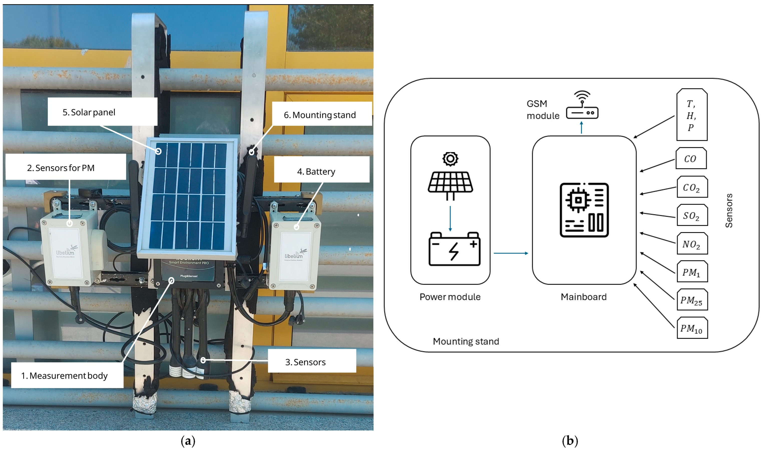
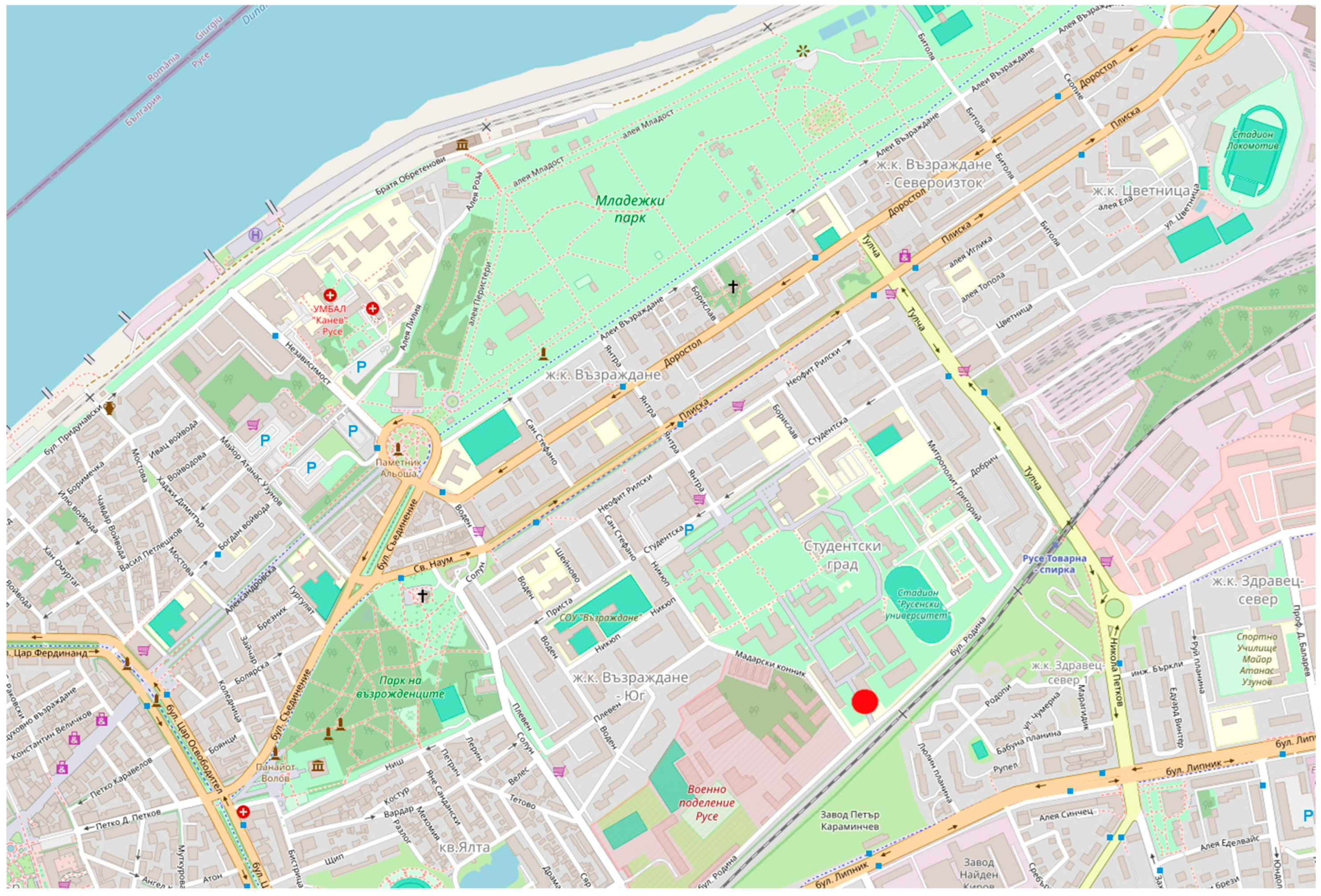
For the purpose of our own research, a national initiative has been implemented in Bulgaria through the University of Ruse, “Angel Kanchev”. As part of the Bulgarian National Recovery and Resilience Plan (project BG-RRP-2.013-0001), co-financed by the European Union under the NextGenerationEU mechanism, the university deployed a high-resolution, autonomous air quality monitoring platform. The system, based on Libelium’s portable sensing technology, was installed near Rodina Boulevard in Ruse and operated continuously from 1 March 2024 to 30 March 2025. It recorded 15 min measurements of CO, CO₂, NO₂, SO₂, PM₁, PM_2.5, PM₁₀, temperature, humidity, and pressure. The platform is powered by a solar panel, supported by a rechargeable battery, and transmits data via GSM to the Libelium Cloud for visualization and analysis.

Measurement locations in the City of Ruse were selected due to their location in the Danube Valley, which is conducive to temperature inversions and the accumulation of pollutants, their proximity to major traffic arteries and residential areas, which reflects the residents’ exposure, and the existing facilities of the technical university, which allowed for the stable installation and maintenance of the platform for a year. Alternative locations, such as industrial zones or rural areas, do not reflect the typical urban exposure experienced by most metropolitan residents. In turn, selecting multiple measurement points would significantly increase operational costs and require additional personnel and complex logistics.

The measurement platform was built using modern IoT sensors, which allowed us to reduce the cost of its implementation significantly. To better illustrate the differences between our platform and traditional reference stations, the following summarizes the main features of both measurement systems.

Table 1. Comparison of the features of reference networks and IoT sensors.

Feature	Reference Networks	IoT Sensors
Installation cost	very high (>EUR 100,000)	low (<EUR 2000)
Accuracy	very high	moderate (requires calibration)
Spatial resolution	low (few points in a city)	high (deployability)
Temporal resolution	usually every 1 h	every few minutes
Cloud integration	limited	full (API, online visualizations)
Power	main power supply	main power supply, accumulator power supply; possible solar power supply

considers the cost, accuracy, mobility, frequency of measurements, and data system integration capabilities.

The above comparison shows that classical reference stations provide the highest measurement accuracy, but their use is limited due to high costs, low mobility, and a limited number of locations. IoT sensors, on the other hand, despite their lower precision, offer exceptional flexibility, low deployment costs, and the ability to build a dense, distributed measurement network.

In practice, the best results are achieved through the complementary use of the two systems, where reference stations act as calibration and validation points. At the same time, IoT sensors enable the tracking of pollution variability at the micro-environmental scale. This approach supports constructing modern, adaptive air quality management systems based on real data and predictive analysis.

Including an Internet of Things (IoT) component in air quality research is an essential step toward a more individualized and spatially sensitive approach to monitoring the urban environment. As shown in Section 1, these solutions enable more accurate mapping of temporal and spatial phenomena and offer the potential for integration with modern data analysis and artificial intelligence tools.

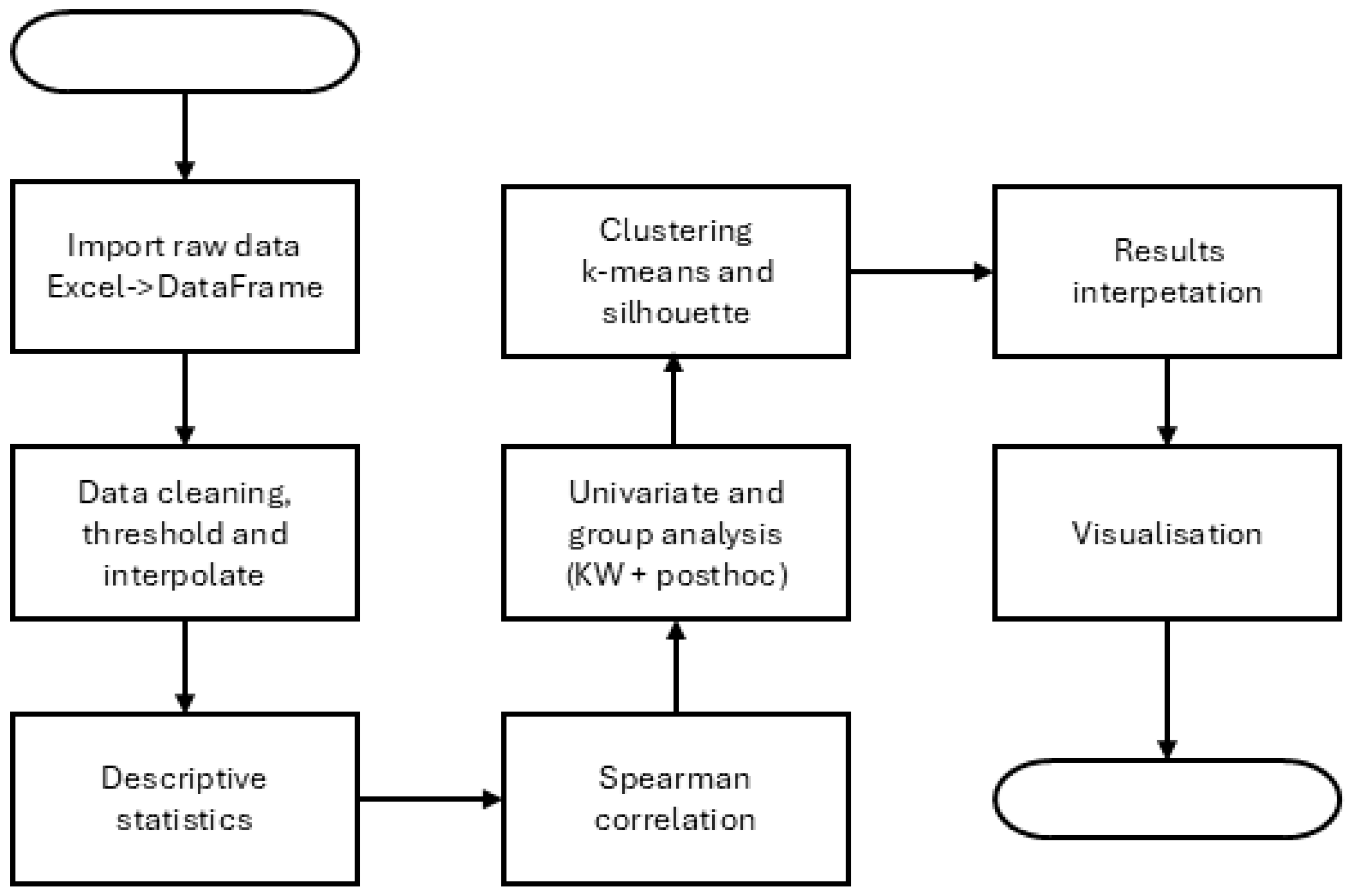
In this article, starting from a review of the existing literature and identified research gaps, the authors focus on implementing an autonomous IoT platform in a central European medium-sized city. Particular emphasis is placed on evaluating the effectiveness of a single measurement point, analyzing temporal variability, and using non-parametric and exploratory methods (Kruskal–Wallis test and k-means clustering) to identify pollution patterns.

The following chapters present the detailed measurement methodology, the analytical tools used, and the interpretation of the results about the hypotheses and current decision-making needs in environmental and urban policy.

2. Materials and Methods

2.1. Monitoring System and Data Collection

The system (Figure 1) is placed at a height of 2 m in the yard of the University of Ruse near the Boulevard “Rodina” (Figure 2). It consists of a measuring body (1) to which the measuring sensors are connected, divided into two groups. One group is combined and in a common body, designated as sensors for PM (2), and the second group comprises sensors (3) that are individually connected to the measuring body. The device is powered by a battery (4) that is charged by the sun via a solar panel (5). The measured data are recorded in the device and transmitted via the GSM network of a mobile operator to the cloud of the company Libelium (Zaragoza, Spain). There, the data are stored in the “Libelium Cloud”, a cloud platform. All recorded data can be downloaded, saved onto a computer, and processed with Microsoft Excel (version 365). It can also be visualized in the cloud platform by presenting it in a graphical form. The entire system is mounted on a stand next to the window of a building at the University of Ruse with a mounting stand (6). The GPS coordinates are 43.851607° N, 25.973332° E. Measurements were conducted near busy highways and a railway junction, which also contributes to the interpretation of the results. Data processing and analysis were conducted using custom-written Python 3.9 scripts (see link https://github.com/aczerepicki-pw/ruse_measurements, accessed on 24 May 2025).

Every sensor has specific technical data [19].

Temperature sensor:

• Operational range: −40~+85 °C;
• Full accuracy range: 0~+65 °C, accuracy: ±1 °C.

Humidity sensor:

• Measurement range: 0~100% of relative humidity;
• Accuracy: <±3% RH (at 25 °C, range 20~80%);
• Hysteresis: ±1% RH, operating temperature: −40~+85 °C.

Pressure sensor:

• Measurement range: 30~110 kPa;
• Operational temperature range: −40 ~ + 85 °C;
• Absolute accuracy: ±0.1 kPa (0~65 °C).

All sensors are calibrated by the company. The measurements are performed 24 h a day, 365 days a year. The data are transmitted to the Libelium cloud every 15 min.

Figure 3 illustrates the structure of this study in the form of a sequence of the most important stages, consisting of data acquisition from the measurement system, data preprocessing, statistical analysis, and interpretation and visualization of the study results.

2.2. Data Preprocessing

Time-grid synchronization: All observations were aligned to a common timestamp index.

Range filtering: Readings outside instrument detection limits were flagged and removed.

Data cleaning: Readings outside instrument detection limits were flagged and removed. Prior to any statistical analysis, all sensor channels were checked for physically implausible or spurious values, and these were replaced through linear interpolation of the nearest valid observations. The following rules were applied to each channel:

• CO₂: any measurement equal to zero (0 ppm) was deemed non-physical and replaced using linear interpolation between the closest non-zero neighbors;
• CO: readings ≤ 0.1 ppm were considered to be below the sensor’s reliable detection limit; these values were replaced by linear interpolation, and any remaining NaNs were then dropped;
• Humidity: missing values (NaN) and any values below 15% relative humidity were replaced by linear interpolation;
• NO₂: values ≥ 60 ppb (beyond the sensor’s upper specification) were replaced by linear interpolation;
• SO₂: values ≤ 0.1 ppb or ≥ 1.2 ppb (outside the sensor’s plausible range) were replaced by linear interpolation.

All interpolations were carried out on the time-ordered series using a simple 1D linear method. After interpolation, any residual NaNs in CO were removed by dropping those rows.

Fusion: Cleaned data were merged into a single working dataset.

Reference: The methodology for preprocessing follows procedures in [20,21].

2.3. Descriptive Statistics

For each variable, we computed the mean, median, standard deviation, minimum, and maximum values. Histograms and quantile–quantile plots were used to assess distribution shape (skewness and kurtosis). Variables with non-symmetric distributions were marked for non-parametric analysis.

2.4. Categorical Temporal Variables

We derived the following categorical features:

• Day of the week (1 = Sunday… 7 = Saturday);
• Part of the day (“Night”: 00–06 h; “Morning”: 06–12 h; “Afternoon”: 12–18 h; “Evening”: 18–24 h);
• Season (Winter, Spring, Summer, Autumn);
• Day type (Working day, Holiday).

2.5. Correlation Analysis

Spearman’s rank correlation coefficients (ρ) were calculated for all variable pairs to assess monotonic relationships. Significance was evaluated at α = 0.05. Correlations were interpreted as: |ρ| < 0.3 (negligible), 0.3–0.5 (moderate), 0.5–0.7 (strong), or >0.7 (very strong).

2.6. Non-Parametric Tests

The Kruskal–Wallis H test was used to compare median pollutant levels across groups, defined by the day of the week and the part of the day. This non-parametric test is suitable for comparing three or more independent groups when the assumptions of normality and homogeneity of variance are not met.

The rationale for choosing the Kruskal–Wallis test is as follows:

• Non-normal distribution: Preliminary analysis indicated that the distributions of PM₁₀ and other pollutants did not conform to a normal distribution, as confirmed by the Shapiro–Wilk test (p < 0.05);
• Heteroscedasticity: Levene’s test for equality of variances revealed significant differences in variances across groups (p < 0.05), violating one of the key assumptions of ANOVA;
• Ordinal data: The Kruskal–Wallis test is appropriate for ordinal data or continuous data that do not meet the assumptions of parametric tests.

Where the H test indicated significance (p < 0.05), post hoc pairwise comparisons were performed, using Dunn–Sidak correction to control the family-wise error rate.

2.7. Feature Selection and Clustering

Based on the cumulative significance from post hoc tests and correlation strength, three key pollutants (PM₁₀, PM_2.5, and CO) were selected as characteristic features. To explore joint patterns with meteorological variables (temperature, humidity, pressure, SO₂, and NO₂), we applied k-means clustering. The optimal number of clusters was determined using the Elbow method and silhouette analysis. Cluster profiles were described using the mean values of all variables.

2.8. Software

All analyses were performed in Python 3.9, using pandas for data handling, SciPy (version 1.11.4) and stats models for statistical tests, and scikit-learn (version 1.3.2) for clustering. Visualization was produced with matplotlib (version 3.7.3) and seaborn (version 0.12.2).

3. Results

3.1. Descriptive Statistics Results

Table 2. Descriptive statistics (mean, median, standard deviation, and min–max).

Variable	Unit	Mean	Median	Std. Dev.	Min	Max
CO2	ppm	413.267	405.554	54.182	213.005	1567.565
CO	ppm	0.486	0.387	0.497	0.100	14.770
Humidity	%	63.379	62.076	27.007	15.005	100.000
NO2	ppm	0.038	0.000	0.969	0.000	54.325
Pressure	Pa	101,197	101,066	748	98,581	103,292
SO2	ppm	0.366	0.367	0.045	0.100	1.911
PM1	µg	5.488	2.270	9.084	0.030	118.470
PM2.5	µg	10.481	5.000	19.709	0.030	553.150
PM10	µg	34.443	10.670	228.528	0.030	10,377.010
Temperature	°C	14.896	15.000	10.247	−5.000	38.000

summarizes the basic statistics for all measured variables. Concentrations of CO₂ and meteorological parameters fall within expected ambient ranges, whereas episodic peaks are observed for CO, NO₂, SO₂, and particulate matter.

Figure 4a shows the time course of the quantity. The graph shows a time window in which the measured CO₂ values are high. It follows that reaching the maximum value should not be considered an outlier. Figure 4b shows the histogram of the variable.

Figure 5a shows the time course of the quantity. The graph shows a time window in which the measured PM_2.5 values are high. It follows that reaching the maximum value should not be considered an outlier. Figure 5b shows the histogram of the variable.

Figure 6a shows the time course of the quantity. The graph shows a time window in which the measured PM₁₀ values are high. It follows that reaching the maximum value should not be considered an outlier. Figure 6b shows the histogram of the variable.

Histograms and Q–Q plots reveal that CO₂, humidity, pressure, and SO₂ approximate symmetric distributions, whereas CO, NO₂, PM₁, PM_2.5, and PM₁₀ are right-skewed with heavy tails. In particular, PM₁₀ exhibits extreme maximum values (>10⁴ µg m⁻³), indicating occasional pollution events.

3.2. Spearman Rank Correlation

Because many distributions depart from normality, Spearman’s rank correlation (ρ) was used. Figure 7 displays the correlation matrix heatmap.

Table 3. Spearman correlation matrix according to the following scale: 0—no dependence (0 ≤ |ρ| < 0.3), 0.5—moderate dependence (0.3 ≤ |ρ| < 0.5), 0.7—strong dependence (0.5 ≤ |ρ| < 0.7), 1—very strong dependence (0.7 ≤ |ρ| ≤ 1).

	CO2	CO	Humidity	NO2	Pressure	SO2	PM1	PM2.5	PM10	Temperature
CO2	-	−0	−0.5	−0.5	−0	−0	−0	−0	−0	0.5
CO	−0	-	0.7	0.7	0.5	1	0.7	0.7	0	−1
Humidity	−0.5	0.7	-	0.5	0	0.7	0.7	0.7	0	−1
NO2	0.5	0.7	0.5	-	0.5	0.7	0.5	0.5	0	−0.7
Pressure	−0	0.5	0	0.5	-	0.5	0	0	0	−0.5
SO2	−0	1	0.7	0.7	0.5	-	0.7	0.7	0	−1
PM1	−0	0.7	0.7	0.5	0	0.7	-	1	0.7	−0.7
PM2.5	−0	0.7	0.7	0.5	0	0.7	1	-	1	−0.5
PM10	−0	0	0	0	0	0	0.7	1	-	−0
Temperature	0.5	−1	−1	−0.7	−0.5	−1	−0.7	−0.5	−0	-

highlights selected ρ values and significance (all p < 0.001).

Key findings:

• Very strong positive inter-correlation among particulate fractions: ρ(PM_2.5, PM₁₀) = 0.85, ρ(PM₁, PM_2.5) = 0.80,
• Moderate to strong correlations between gaseous pollutants: ρ(CO, SO₂) = 0.72, ρ(CO, NO₂) = 0.65
• Temperature is inversely correlated with humidity (ρ = −0.75) and particulate matter: ρ(PM₁₀, T) = −0.60, suggesting enhanced dispersion in warmer, drier conditions.

3.3. Effect of the Day of the Week

A Kruskal–Wallis H test for PM₁₀ yields H = 191.57, p < 10⁻³⁷, indicating significant differences across weekdays (

Table 4. Kruskal–Wallis test results for PM10 depending on the day of the week (p < 10⁻³⁷).

Source	SS	df	MS	Chi-sq	Prob > Chi-sq
Groups	1.00 × 1010	6	1.67 × 109	191.57	1.18 × 10−38
Error	1.31 × 1012	25,082	5.21 × 107
Total	1.32 × 1012	25,088

). Post hoc Dunn–Sidak comparisons (

Table 5. Post hoc analysis test decision for the dependence of air quality on the day of the week: 0—no statistically significant difference between distributions, 1—there is a statistically significant difference between distributions.

Group 1	Group 2	CO2	CO	Humidity	NO2	Pressure	SO2	Group 1	Group 2	CO2	CO
1	2	0	1	0	0	1	0	0	1	1	0
1	3	0	0	0	0	1	0	0	1	1	0
1	4	1	1	1	0	0	1	0	1	1	0
1	5	0	1	1	0	0	1	0	1	1	0
1	6	1	1	1	0	0	1	0	1	1	0
1	7	0	0	0	0	0	0	0	0	0	0
2	3	0	0	0	0	0	0	0	0	1	0
2	4	0	0	1	1	0	0	0	0	0	0
2	5	0	1	1	0	0	0	0	0	1	0
2	6	0	0	1	0	1	0	0	0	0	0
2	7	0	1	0	0	1	0	0	1	1	0
3	4	0	0	1	0	1	1	1	0	1	0
3	5	0	1	1	0	1	1	0	0	1	0
3	6	0	1	1	0	1	1	1	0	1	0
3	7	0	0	0	0	1	0	0	1	1	0
4	5	0	1	0	0	0	0	0	0	0	0
4	6	0	0	0	1	0	0	0	0	0	0
4	7	1	1	1	1	1	1	1	1	1	0
5	6	0	0	0	0	0	0	0	0	1	0
5	7	0	1	1	0	1	1	0	1	1	0
6	7	0	1	1	0	0	1	1	1	1	0

) show that Sunday’s median PM₁₀ differs from Monday–Friday (all adjusted p < 0.001), while Saturday resembles Sunday (p > 0.05). The box plots in Figure 8 illustrate these patterns for the PM₁₀ contamination case.

3.4. Effect of the Time of Day

To further investigate the influence of time on pollutant concentrations, the data were grouped into the four parts of the day: night, morning, afternoon, and evening. The Kruskal–Wallis tests conducted on all pollutants yielded significant results ($p<{10}^{-10}$).

For SO₂, concentrations during the night differed significantly from those in the morning, afternoon, and evening (all Dunn–Sidak $p<0.001$). Similar temporal trends were observed for CO, PM_2.5, and PM₁₀, indicating that the time of day has a substantial effect on air quality (Figure 9).

Table 6. Test decision of post hoc analysis for the dependence of air quality on the part of the day: 0—no statistically significant difference between distributions, 1—there is a statistically significant difference between distributions.

Group 1	Group 2	CO2	CO	Humidity	NO2	Pressure	SO2	Group 1	Group 2	CO2	CO
1	2	1	1	1	1	0	1	1	1	1	1
1	3	1	1	1	1	1	1	1	1	1	1
1	4	1	0	1	0	0	1	1	1	1	1
2	3	1	1	1	1	1	1	1	0	1	1
2	4	1	1	1	1	1	1	1	1	1	1
3	4	0	1	1	0	1	1	1	1	1	1

summarizes the results of the post hoc analysis for the dependence of air quality on the time of day, showing significant differences across various pollutants.

3.5. Clustering of Pollution Profiles

Based on the cumulative post hoc significance and Spearman ρ, three key pollutants (PM₁₀, PM_2.5, and CO) were selected for clustering with meteorological variables. K-means (k = 4) reveals four distinct profiles (

Table 7. Air pollution profiles.

Cluster	Abundance	PM2.5	PM10	CO	Temperature	Humidity	Pressure	SO2	NO2
		Key Variables			Meteorological Parameters			Dependent Variables
1	12,242	15.119	31.351	0.62065	8477	85	1.02 × 105	0.3428	0.0089
2	12,595	4.6974	15.346	0.35402	25.658	42.374	1.01 × 105	0.3918	0.0225
3	12	16.692	30.809	0.65338	10.956	74.061	1.02 × 105	0.3929	25.1182
4	93	194.52	3076.7	0.69822	0.22505	99.453	1.01 × 105	0.4181	0.0269

Cluster 1 (winter-like): moderate PM levels, low temperature, and high humidity. Cluster 2 (summer-like): low PM and CO, high temperature, and low humidity. Cluster 3 (NO₂ spikes): normal PM but extreme NO₂, likely local emission events. Cluster 4 (pollution episodes): very high PM, near-freezing temperature, and saturated humidity, indicative of inversion or industrial incidents.

).

Figure 10 presents the box plots of cluster distributions. Figure 11 presents a time series annotated by clusters for the inclusion of PM₁₀ contamination.

4. Discussion

The results obtained from one-year high-frequency air quality monitoring in the city of Ruse provide valuable insights into the spatiotemporal dynamics of pollutant concentrations in urban environments. The autonomous measurement system implemented under the National Recovery and Resilience Plan of Bulgaria (project BG-RRP-2.013-0001), co-financed by the European Union through the NextGenerationEU initiative, demonstrates the feasibility and utility of solar-powered, IoT-enabled platforms for environmental data acquisition and analysis.

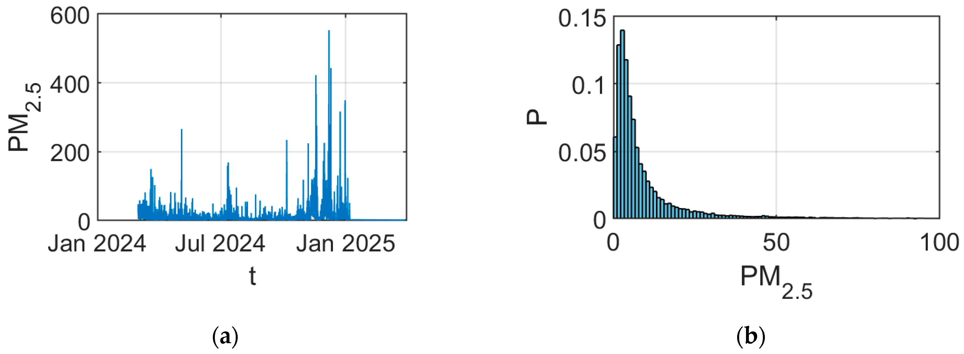
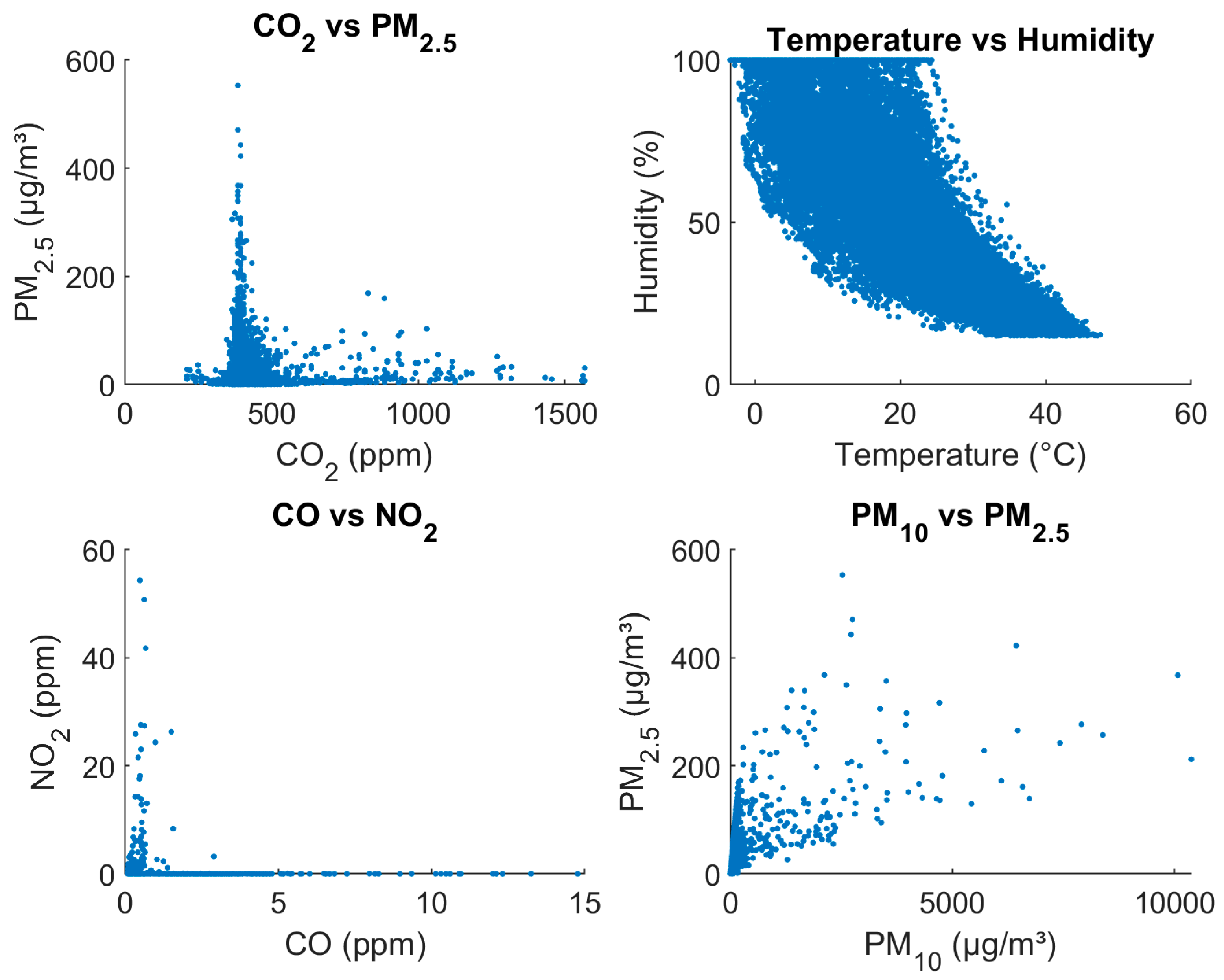
The descriptive statistics and correlation analyses confirm expected patterns of pollutant variability and interdependence. Very strong positive correlations were observed among particulate matter fractions (e.g., PM_2.5 and PM₁₀), aligning with findings from previous studies conducted in urban areas in Central and Eastern Europe [1,3]. These results suggest a commonality in emission sources, such as residential solid fuel combustion and traffic-related particulate emissions, consistent with Polish national inventories [5]. The moderate to strong correlations between gaseous pollutants (e.g., CO–NO₂ and CO–SO₂) and the inverse correlation of temperature with PM concentrations support the hypothesis that meteorological factors modulate pollutant dispersion and accumulation, especially during cold seasons when inversion layers often trap pollutants near the ground [6,7,22].

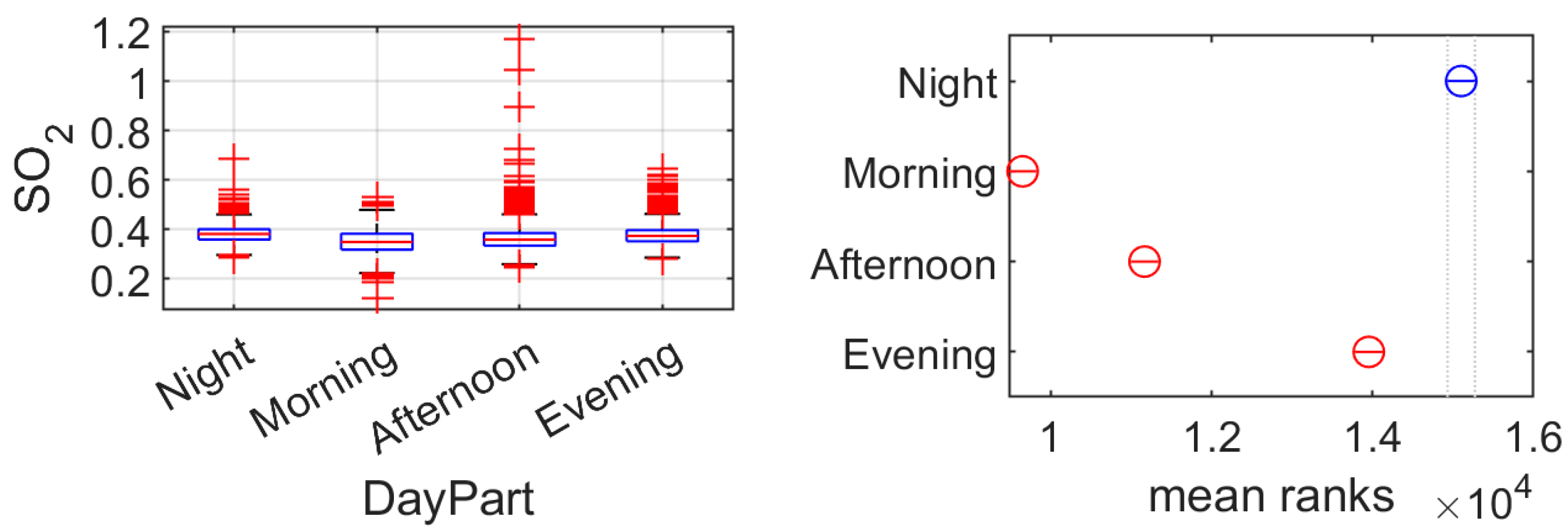
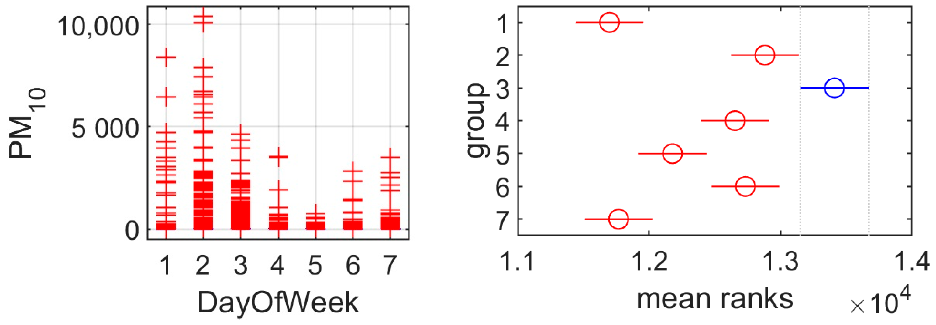
The use of non-parametric statistical methods, such as the Kruskal–Wallis test and Dunn–Sidak post hoc comparisons, allowed for a robust assessment of temporal heterogeneity in pollutant levels. Similar methodologies have been applied successfully in studies from Italy [23], India [24], and Romania [25], validating their relevance in the context of non-normally distributed environmental data. The identification of statistically significant differences in PM₁₀ and PM_2.5 concentrations across days of the week and parts of the day reflects both human activity rhythms and atmospheric boundary layer dynamics. The highest concentrations were typically recorded in the early morning and evening hours, consistent with periods of increased vehicular traffic and lower atmospheric mixing [26,27].

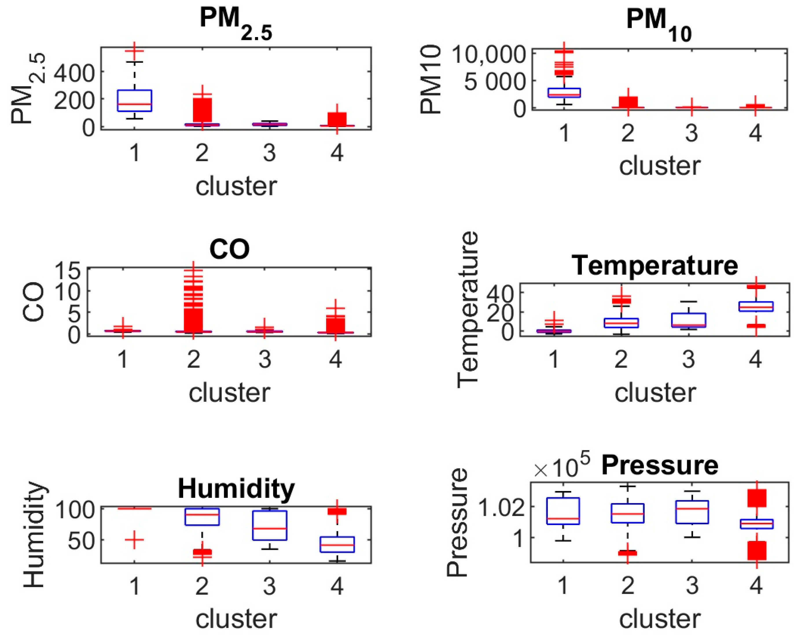
The k-means clustering analysis yielded four distinct pollution profiles, which we interpret as follows. Cluster 1 represents a typical winter scenario with low temperatures and elevated PM concentrations due to residential heating; Cluster 2 corresponds to summer conditions with higher temperatures and improved air dispersion; Cluster 3 reflects episodic NO₂ spikes, likely due to traffic congestion or local combustion events; and Cluster 4 captures extreme pollution episodes, possibly linked to stagnation events or industrial releases. These findings are consistent with previous cluster-based approaches used in cities such as Delhi [28] and Beijing [29], highlighting the potential of unsupervised learning methods in classifying urban air quality patterns.

From a methodological standpoint, the integration of a continuously operating sensor network with cloud-based storage and GSM transmission proved to be highly effective. This approach enables real-time access to high-resolution environmental data, which is essential for developing early warning systems, informing public health interventions, and evaluating policy outcomes. Similar sensor networks have been tested in the CLINSH project in Western Europe [10] and in smart city pilot programs in East Asia [30], underscoring the growing importance of decentralized, scalable monitoring infrastructure.

Moreover, the reliability of the Libelium-based measurement system was maintained throughout the entire observation period, with a stable energy supply from the solar panel and efficient data transfer. This supports prior evaluations of autonomous monitoring platforms in low-maintenance deployments [17].

This study contributes to the growing body of literature advocating for adaptive, locally grounded environmental monitoring frameworks in support of regional air quality management. While the current analysis focuses on temporal and meteorological drivers of pollutant variability, future work will integrate emissions inventory data and machine learning techniques to enhance predictive modeling and scenario simulations.

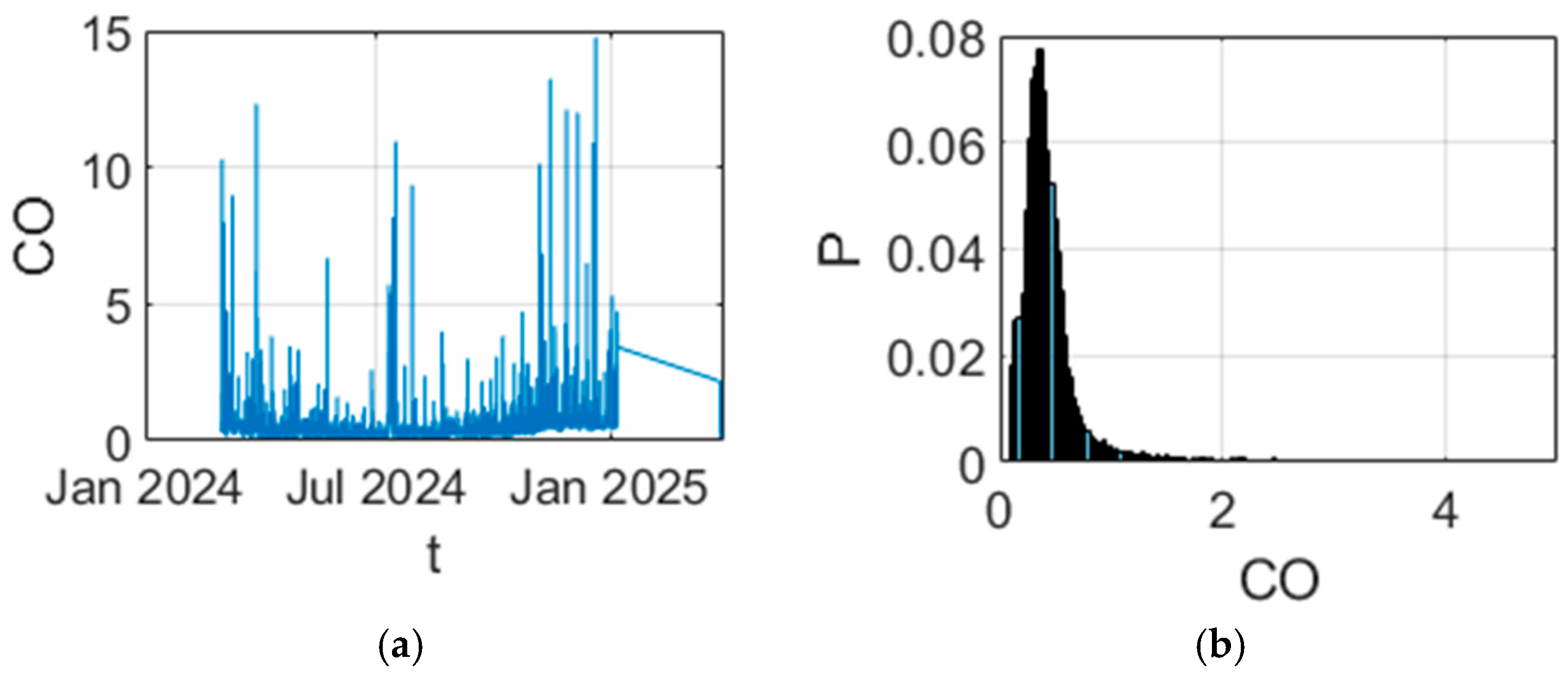
Descriptive statistics revealed episodic pollution peaks for CO, NO₂, SO₂, and particulate matter, while Spearman correlations highlighted strong interdependencies among pollutant species and inverse relationships with temperature and humidity. Non-parametric tests confirmed that median pollutant levels vary significantly by the day of the week and time of day, reflecting socio-economic rhythms (e.g., traffic and industrial operations). Clustering key pollutants (PM₁₀, PM_2.5, and CO) with meteorological variables yielded four distinct profiles, including a “winter-like” cluster, a “summer-like” clean air cluster, an NO₂ spike cluster, and a high-pollution inversion cluster. These findings underscore the need for adaptive monitoring and targeted emission reduction measures tied to specific temporal and meteorological scenarios.

5. Conclusions

This study demonstrated the effectiveness of a fully autonomous, solar-powered air quality monitoring system implemented by the University of Ruse, “Angel Kanchev”, as part of the Bulgarian National Recovery and Resilience Plan. The use of Libelium’s modular platform enabled the continuous measurement of key air pollutants (CO, CO₂, NO₂, SO₂, PM₁, PM_2.5, and PM₁₀) and meteorological variables (temperature, humidity, and pressure) at high temporal resolution over a 12-month period. The system’s integration of GSM data transmission and cloud-based storage proved to be robust, reliable, and suited for long-term urban deployment.

From a data analysis perspective, the following conclusions can be drawn:

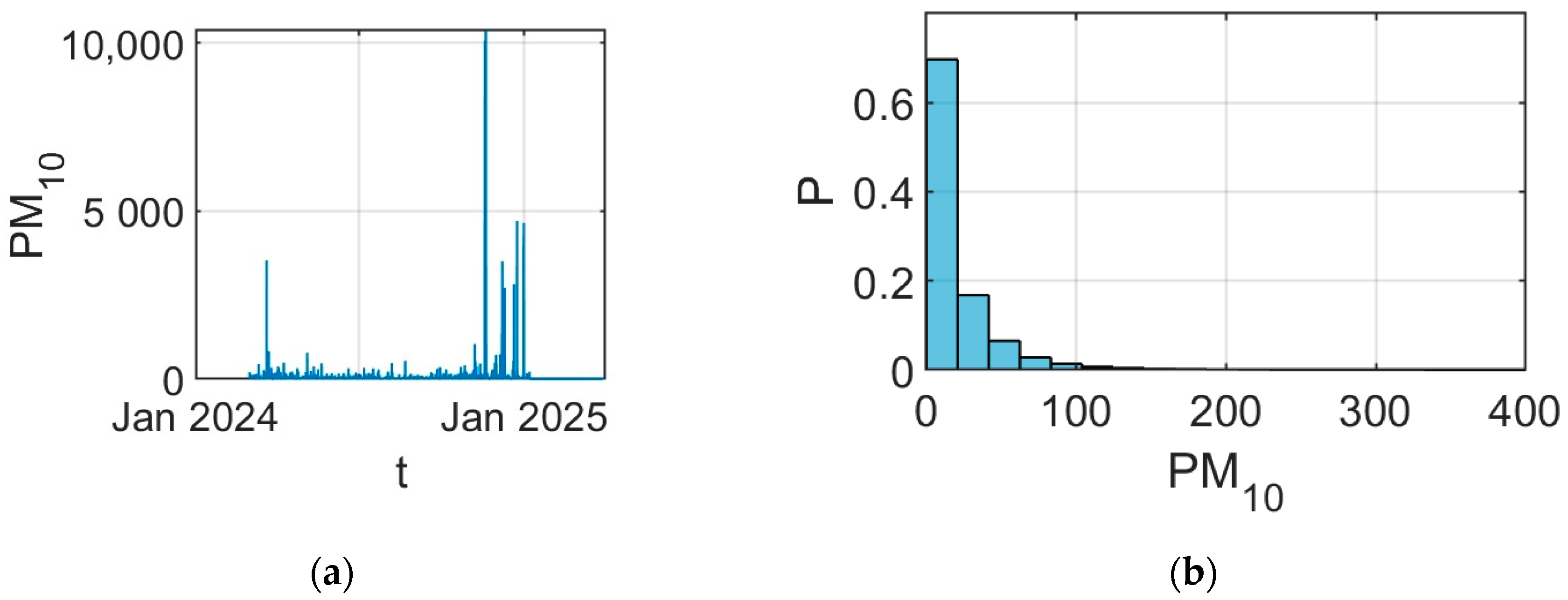
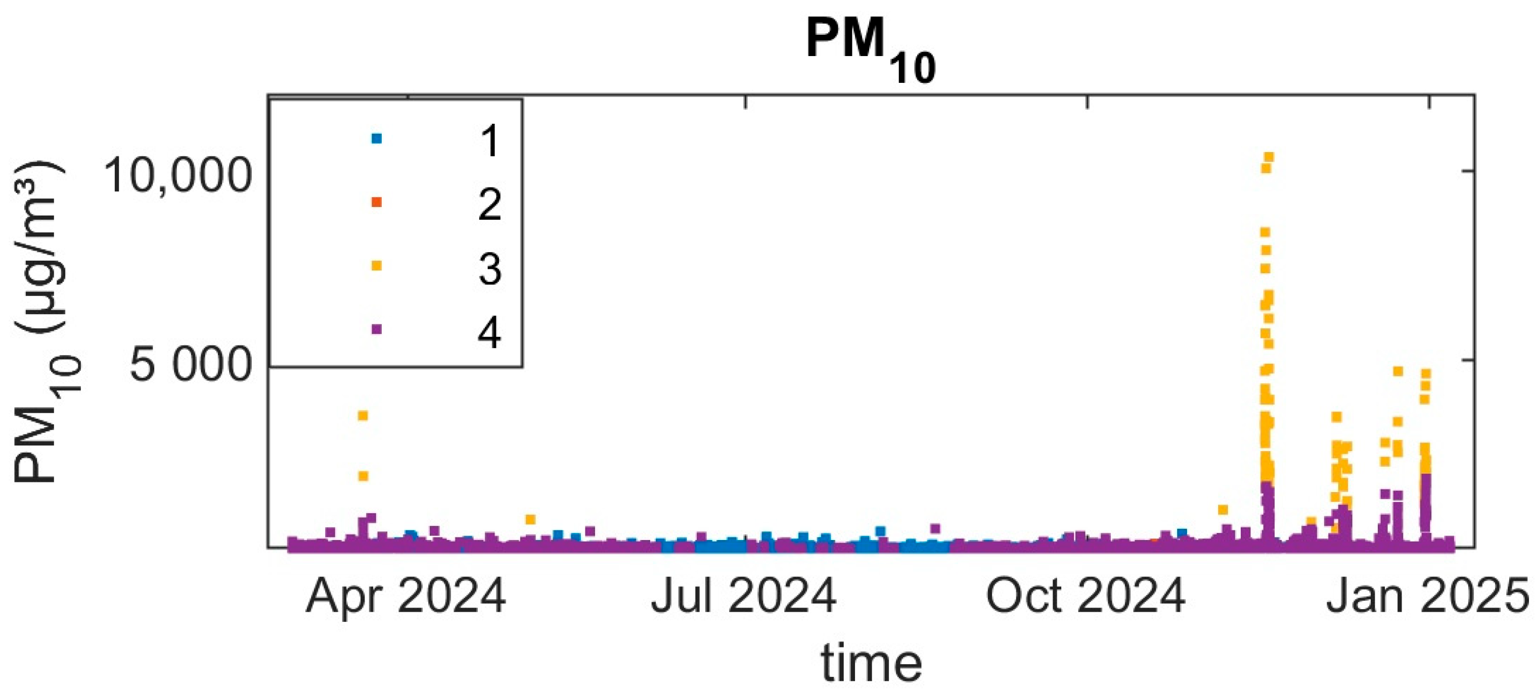
• Pollutant distributions exhibit high asymmetry and heavy-tailed behavior, particularly for PM₁₀, where extreme values point to episodic pollution events associated with unfavorable atmospheric conditions;
• Spearman rank correlations revealed strong interdependencies among particulate fractions and significant negative associations with temperature, confirming the role of meteorological variables in pollutant dynamics;
• Kruskal–Wallis and Dunn–Sidak tests identified statistically significant differences in pollutant levels by the day of the week and time of day, reflecting human activity cycles and boundary layer effects;
• Unsupervised clustering (k-means) yielded four distinct pollution profiles: cold season accumulation, clean air summer patterns, localized NO₂ peaks, and high-pollution inversion episodes;
• These distinct clusters, together with the system’s uninterrupted year-long operation, demonstrate that measurements from a single, properly placed, and calibrated IoT sensor are sufficient to identify and monitor typical urban air quality scenarios.

These findings not only confirm the reliability and precision of the deployed monitoring infrastructure but also illustrate the added value of integrating environmental sensing with non-parametric statistics and machine learning approaches. The system’s portability, autonomy, and real-time data access make it an attractive model for other urban regions seeking to expand air quality surveillance capabilities.

Future research will focus on the predictive modeling of air quality based on meteorological inputs and human activity proxies. Time-series decomposition (e.g., STL and ARIMA), multivariate regression, and deep learning methods such as LSTM will be explored to forecast pollutant concentrations and identify leading indicators of acute air quality deterioration. Integration with traffic flow and energy usage datasets may further enhance the interpretability of pollution patterns and guide targeted mitigation strategies in real time.

Limitations and Generalisability

Despite the strengths of our year-long, high-frequency monitoring campaign, several limitations should be noted. First, all measurements derive from a single sensor node located on the university campus; micro-scale factors (local traffic density, building-induced turbulence, and street canyon effects) may therefore cause biases regarding absolute pollutant levels and temporal patterns. Second, although the Libelium platform was factory-calibrated and proven to be stable over 12 months, the lack of concurrent reference station collocation means that potential sensor drift or cross-sensitivities cannot be fully excluded. Third, the dataset spans only one annual cycle. Inter-annual variability (e.g., unusually cold winters, extended heatwaves, and episodic industrial emissions) may yield slightly different cluster structures or temporal contrasts. Fourth, our meteorological dataset omitted wind speed, wind direction, and solar radiation, all of which can strongly influence pollutant dispersion and secondary aerosol formation; inclusion of these parameters could refine cluster definitions and improve predictive models. With regard to generalizability, the core methodology—deployment of a single, solar-powered IoT node coupled with non-parametric tests and k-means clustering—can readily be adopted in other mid-sized European cities exhibiting similar continental climates and diurnal traffic cycles. However, local topography, emission source profiles, and urban morphology will affect the number and character of identifiable pollution clusters. Any replication should therefore include initial site-specific validation (ideally via short-term co-location with reference instruments), as well as the adaptation of clustering features to local emission sources and meteorological regimes. In sum, while our results convincingly demonstrate the potential of a lone IoT sensor for capturing dominant urban air quality scenarios, extension to broader spatial networks and longer observation periods will be essential to fully characterize city-wide and year-to-year variability.

References

1. de Bont, J.; Jaganathan, S.; Dahlquist, M.; Persson, Å.; Stafoggia, M.; Ljungman, P. Ambient Air Pollution and Cardiovascular Diseases: An Umbrella Review of Systematic Reviews and Meta-analyses. J. Intern. Med. 2022, 291, 779–800. [Google Scholar] [CrossRef] [PubMed]
2. Institute for Health Metrics and Evaluation (IHME). 2024 Global Burden of Disease 2021: Findings from the GBD 2021 Study; IHME: Seattle, WA, USA, 2024. Available online: https://www.healthdata.org/research-analysis/library/global-burden-disease-2021-findings-gbd-2021-study (accessed on 30 June 2025).
3. de Paula Santos, U.D.P.; Arbex, M.A.; Braga, A.L.F.; Mizutani, R.F.; Cançado, J.E.D.; Terra-Filho, M.; Chatkin, J.M. Environmental Air Pollution: Respiratory Effects. J. Bras. Pneumol. 2021, 47, e20200267. [Google Scholar] [CrossRef]
4. World Health Organization. WHO Global Air Quality Guidelines: Particulate Matter (PM2.5 and PM10), Ozone, Nitrogen Dioxide, Sulfur Dioxide and Carbon Monoxide. Available online: https://www.who.int/publications/i/item/9789240034228 (accessed on 30 June 2025).
5. KOBIZE (National Balancing and Emission Management Centre). National Emissions Balance SO2, NOx, CO, NH3, NMLZO, PM, Heavy Metals and Pops; KOBiZE: Warsaw, Poland, 2020. [Google Scholar]
6. European Environment Agency. Air Quality in Europe 2021. Available online: https://www.eea.europa.eu/publications/air-quality-in-europe-2021 (accessed on 30 June 2025).
7. Zhang, J.; Liu, Z.; Tian, B.; Li, J.; Luo, J.; Wang, X.; Ai, S.; Wang, X. Assessment of Soil Heavy Metal Pollution in Provinces of China Based on Different Soil Types: From Normalization to Soil Quality Criteria and Ecological Risk Assessment. J. Hazard. Mater. 2023, 441, 129891. [Google Scholar] [CrossRef] [PubMed]
8. Yuan, R.; Ma, Q.; Zhang, Q.; Yuan, X.; Wang, Q.; Luo, C. Coordinated Effects of Energy Transition on Air Pollution Mitigation and CO2 Emission Control in China. Sci. Total Environ. 2022, 841, 156482. [Google Scholar] [CrossRef] [PubMed]
9. Angon, P.B.; Islam, M.S.; KC, S.; Das, A.; Anjum, N.; Poudel, A.; Suchi, S.A. Sources, Effects and Present Perspectives of Heavy Metals Contamination: Soil, Plants and Human Food Chain. Heliyon 2024, 10, e28357. [Google Scholar] [CrossRef]
10. European Climate, Infrastructure and Environment Executive Agency (CINEA). CLean INland Shipping. Available online: https://webgate.ec.europa.eu/life/publicWebsite/project/LIFE15-ENV-NL-000217/clean-inland-shipping/ (accessed on 30 June 2025).
11. Hasenfratz, D.; Saukh, O.; Sturzenegger, S.; Thiele, L. Participatory Air Pollution Monitoring Using Smartphones. Mob. Sens. 2012, 1, 1–5. [Google Scholar]
12. Morawska, L.; Thai, P.K.; Liu, X.; Asumadu-Sakyi, A.; Ayoko, G.; Bartonova, A.; Bedini, A.; Chai, F.; Christensen, B.; Dunbabin, M.; et al. Applications of Low-Cost Sensing Technologies for Air Quality Monitoring and Exposure Assessment: How Far Have They Gone? Environ. Int. 2018, 116, 286–299. [Google Scholar] [CrossRef]
13. Rai, A.C.; Kumar, P.; Pilla, F.; Skouloudis, A.N.; Di Sabatino, S.; Ratti, C.; Yasar, A.; Rickerby, D. End-User Perspective of Low-Cost Sensors for Outdoor Air Pollution Monitoring. Sci. Total Environ. 2017, 607–608, 691–705. [Google Scholar] [CrossRef]
14. Li, W.; Zhang, Y.; Liu, Y. Multivariate Air Quality Forecasting with Residual Nested LSTM Neural Network Based on DSWT. Sustainability 2025, 17, 2244. [Google Scholar] [CrossRef]
15. Rakib, M.; Haq, S.; Hossain, M.I.; Rahman, T. IoT Based Air Pollution Monitoring & Prediction System. In Proceedings of the 2022 International Conference on Innovations in Science, Engineering and Technology (ICISET), Chittagong, Bangladesh, 26–27 February 2022; pp. 184–189. [Google Scholar]
16. Sung, Y.; Lee, S.; Kim, Y.; Park, H. Development of a Smart Air Quality Monitoring System and Its Operation. Asian J. Atmos. Environ. 2019, 13, 30–38. [Google Scholar] [CrossRef]
17. Snyder, E.G.; Watkins, T.H.; Solomon, P.A.; Thoma, E.D.; Williams, R.W.; Hagler, G.S.W.; Shelow, D.; Hindin, D.A.; Kilaru, V.J.; Preuss, P.W. The Changing Paradigm of Air Pollution Monitoring. Environ. Sci. Technol. 2013, 47, 11369–11377. [Google Scholar] [CrossRef]
18. Choudhary, A.; Kumar, P.; Pradhan, C.; Sahu, S.K.; Chaudhary, S.K.; Joshi, P.K.; Pandey, D.N.; Prakash, D.; Mohanty, A. Evaluating Air Quality and Criteria Pollutants Prediction Disparities by Data Mining along a Stretch of Urban-Rural Agglomeration Includes Coal-Mine Belts and Thermal Power Plants. Front. Environ. Sci. 2023, 11. [Google Scholar] [CrossRef]
19. Libelium Sensors Specification. Available online: https://www.libelium.com/iot-products/plug-sense/#specifications-3 (accessed on 30 June 2025).
20. Kozłowski, M. Assessment of Safety and Ride Quality Based on Comparative Studies of a New Type of Universal Steering Wheel in 3D Simulators. Eksploat. Niezawodn.—Maint. Reliab. 2016, 18, 481–487. [Google Scholar] [CrossRef]
21. Choromański, W.; Grabarek, I.; Kozłowski, M. Research on an Innovative Multifunction Steering Wheel for Individuals with Reduced Mobility. Transp. Res. Part F Traffic Psychol. Behav. 2019, 61, 178–187. [Google Scholar] [CrossRef]
22. Qiu, M.; Zigler, C.; Selin, N.E. Statistical and Machine Learning Methods for Evaluating Trends in Air Quality under Changing Meteorological Conditions. Atmos. Chem. Phys. 2022, 22, 10551–10566. [Google Scholar] [CrossRef]
23. Di Bernardino, A.; Iannarelli, A.M.; Diémoz, H.; Casadio, S.; Cacciani, M.; Siani, A.M. Analysis of Two-Decade Meteorological and Air Quality Trends in Rome (Italy). Theor. Appl. Climatol. 2022, 149, 291–307. [Google Scholar] [CrossRef]
24. Kumar, K.; Pande, B.P. Air Pollution Prediction with Machine Learning: A Case Study of Indian Cities. Int. J. Environ. Sci. Technol. 2023, 20, 5333–5348. [Google Scholar] [CrossRef]
25. Iordache, Ş.; Dunea, D. Cross-Spectrum Analysis Applied to Air Pollution Time Series from Several Urban Areas of Romania. Environ. Eng. Manag. J. 2013, 12. [Google Scholar] [CrossRef]
26. Bherwani, H.; Singh, A.; Kumar, R. Assessment Methods of Urban Microclimate and Its Parameters: A Critical Review to Take the Research from Lab to Land. Urban Clim. 2020, 34, 100690. [Google Scholar] [CrossRef]
27. Sun, Y.; Lu, P.; Qu, B.; Li, J. Resilience Assessment and Influencing Factors Analysis of Water Security System in the Yellow River Basin. Sustainability 2024, 16, 9347. [Google Scholar] [CrossRef]
28. Saksena, S.; Joshi, V.; Patil, R.S. Determining Spatial Patterns in Delhi’s Ambient Air Quality Data Using Cluster Analysis; Environmental Change, Vulnerability, and Governance Series; East-West Center Working Papers; East-West Center: Honolulu, HI, USA, 2002. [Google Scholar]
29. Zhao, Y.; Wang, Q.; Wang, H.; He, F.; Li, H.; Zhai, J.; Liu, R.; Hu, P.; Wang, J. Water Security in Beijing-Tianjin-Hebei Region: Challenges and Strategies. Chinese J. Eng. Sci. 2022, 24, 8. [Google Scholar] [CrossRef]
30. Wong, M.; Wang, T.; Ho, H.; Kwok, C.; Lu, K.; Abbas, S. Towards a Smart City: Development and Application of an Improved Integrated Environmental Monitoring System. Sustainability 2018, 10, 623. [Google Scholar] [CrossRef]
Figure 1. General view (a) and block diagram (b) of the measuring system. The arrows show the direction of the information flow.
Sustainability 17 06260 g001
Figure 2. Location of the measuring system in the city of Ruse (the red point).
Sustainability 17 06260 g002
Figure 3. The structure of this study.
Sustainability 17 06260 g003
Figure 4. Time course of the CO variable (a) and the histogram of the probability distribution (b).
Sustainability 17 06260 g004
Figure 5. Time history of the PM2.5 variable (a) and the probability distribution histogram (b).
Sustainability 17 06260 g005
Figure 6. Time history of the PM10 variable (a) and the probability distribution histogram (b).
Sustainability 17 06260 g006
Figure 7. The correlation matrix heatmap. Each blue dot represents one synchronised, hourly observation.
Sustainability 17 06260 g007
Figure 8. Distributions of PM10 pollution on individual days of the week. Box plot and Dunn–Sidak statistics. Statistically similar groups have the same color.
Sustainability 17 06260 g008
Figure 9. Distributions of PM10 pollution on individual times of the day. Box plot and Dunn–Sidak statistics. Statistically similar groups have the same color.
Sustainability 17 06260 g009
Figure 10. Box plots of cluster distributions.
Sustainability 17 06260 g010
Figure 11. PM10 course with assignment to clusters.
Sustainability 17 06260 g011