Short-Term Forecasting of Crop Production for Sustainable Agriculture in a Changing Climate

Abstract

Globally, crop productive systems exhibit climatic adaptation, resulting in increased overall yields over the past century. Nevertheless, inter-annual fluctuations in production can lead to food price volatility, raising concerns about food security. Within this framework, short-term crop yield predictions informed by climate observations may significantly contribute to sustainable agricultural development. In this study, we discuss the criteria for historical monitoring and forecasting of the productive system response to climatic fluctuations, both ordinary and extreme. Here, forecasting is intended as an assessment of the conditional probability distribution of crop yield, given the observed value of a key climatic index in an appropriately chosen month of the year. Wheat production in the Teramo province (central Italy) is adopted as a case study to illustrate the approach. To characterize climatic conditions, this study utilizes the Standardized Precipitation Evapotranspiration Index (SPEI) as a key indicator impacting wheat yield. Validation has been carried out by means of Monte Carlo simulations, confirming the effectiveness of the method. The main findings of this study show that the model describing the yield–SPEI relationship has time-varying parameters and that the study of their variation trend allows for an estimate of their current values. These results are of interest from a methodological point of view, as these methods can be adapted to various crop products across different geographical regions, offering a tool to anticipate production figures. This offers effective tools for informed decision-making in support of both agricultural and economic sustainability, with the additional benefit of helping to mitigate price volatility.

1. Introduction

What level of yield can we anticipate for this crop this year? This is a question of significant practical and economic relevance. While individual farmers can often offer qualitative assessments (e.g., plentiful, meager, disastrous) for their specific holdings, based on observations of climatic conditions and crop status during critical phenological stages, the challenge escalates when seeking quantitative predictions—for instance, in probabilistic terms—on the provincial, regional, or global scale. At these broader levels, monitoring crop development (e.g., bud break, plant health) becomes logistically demanding. Furthermore, the impact of climatic variations on agricultural systems is intricate and highly variable, contingent on factors such as geographical location, farming practices, and the specific crop under consideration. It is not known a priori whether fluctuations in yield are mainly attributable to average values or to extreme events in temperature and precipitation [1]. Moreover, climatic impacts can manifest both directly and indirectly, with the latter including phenomena like pestilent outbreaks and the spread of plant diseases [1].

Climatic variations can induce instability in both food availability and pricing, thereby posing a significant challenge to food security and carrying significant socioeconomic implications [1,2,3,4]. Within this context, short-term forecasting of crop yields, based on climatic data, assumes substantial importance for enabling effective resource allocation, investment strategies, and mitigation of abrupt price swings, within a framework of sustainable agriculture. In this paper, “short-term” refers to the expected harvest of a specific year, based on climatic conditions observed during key phases of the seasonal growth of the crop, in the same year.

While a substantial body of literature has explored the long-term interactions between climate change and agricultural output [5,6,7,8,9,10,11,12,13,14,15,16,17,18,19], fewer investigations [20,21,22,23,24] have focused on the impacts of short-term climatic fluctuations on crop production. To address this research gap, further investigation is essential to elucidate the temporal dynamics of short-term climatic variability on crop yields and to develop standardized methodologies for monitoring and predicting the response of agricultural production systems.

Particularly beneficial could be forecasts of crop yields expressed in probabilistic terms. In prior work [11,12,13], we conducted statistical analyses examining the yield of grape, olive, and wheat in a region of central Italy (Abruzzo), alongside time series of two aridity indices, the Standardized Precipitation Index (SPI) and the Standardized Precipitation Evapotranspiration Index (SPEI) [25,26,27,28,29], spanning approximately 60 years, from 1952 to 2014. The objective of such studies was to identify temporal shifts in the sensitivity of the crop production system to climatic fluctuations. Within this framework, it is crucial to acknowledge that the crop production system is characterized by a complex interplay of factors, including ecological indicators, technical and engineering solutions, as well as economic variables (related to investments, production costs, financial markets, etc.).

To this aim, Guerriero et al. [13] conceptualized agricultural production as a dynamic system including three primary elements or subsystems: first, the natural ecosystem represented by the cultivated land; second, the suite of technological solutions available to mitigate adverse climatic events; and third, the economic feasibility that enables or constrains the implementation of these technological solutions. Furthermore, this system interacts with all stakeholders involved in the production chain, ranging from distributors and/or storage facilities to investors (including insurance companies and financial traders), and ultimately, the end consumers.

Consequently, the production system is examined here according to a black-box model, focusing on input-output relationships, while acknowledging the existence and interactions of other state variables internal to the system, though not directly quantifying them. The input variables consist of appropriately selected climatic indices and the output variables are represented by crop yield values. In this study, we exemplify the proposed approach by considering the case of wheat yield in the Teramo province of the Abruzzo region. Previous investigations in this area [12,13] identified SPI and SPEI (more specifically, the 3-month SPI/SPEI) as key indicators influencing wheat yield and outlined a long-term monitoring methodology to examine the relationship between climatic fluctuations and yield variability. This approach enables the detection of evolving correlations with specific climatic indices, which can be interpreted as temporal shifts in the production system’s sensitivity. It also supports the identification of the most vulnerable phenological stages and, consequently, the climatic indices that are gaining increasing influence over time.

In the present study, we illustrate a short-term probabilistic yield forecasting methodology that builds upon the aforementioned long-term monitoring procedure. With this approach, once the key climatic index has been identified through the monitoring process, the probability distribution of crop yield for the upcoming harvest can be estimated based on current observations of that index. For instance, if long-term monitoring reveals that the 3-month SPEI (denoted as SPEI3) in March is the most impactful on wheat yield, then, by observing this index in March, it is possible to determine the probability distribution of the upcoming harvest, which will occur in late summer.

From the viewpoint of sustainability of agriculture and related economic systems, such a forecast can play a key role in preparing all stakeholders involved in the wheat (or other crop) production/consumption chain, including financial markets, for particularly unfavorable or even favorable production scenarios. Indeed, it is important to highlight that even a particularly abundant harvest can lead to potential problems, such as sudden reductions in market prices that may benefit consumers but disadvantage producers and distributors, as well as financial markets. In this context, anticipating production data is useful for identifying possible future market scenarios, including extreme ones, thereby reducing the “surprise” effect of unexpected production.

According to Tran et al. [22], climate change is expected to increase the overall variability of crop yields over time, which in turn may amplify price volatility in commodity crop markets. In this context, probabilistic yield forecasts issued some months in advance can help with smooth price fluctuations, reducing market turbulence and contributing to the sustainability of commodity crop markets. Moreover, access to the forecasted yield probability distribution can enable data-driven risk analysis for investors (e.g., banks, insurance companies, farms or agribusinesses) and policymakers. By way of example, stakeholders can estimate the probability that the upcoming harvest—either in a specific region or on a global scale—will fall below or exceed a given threshold, or determine the extreme yield values likely to be surpassed with a specified probability level.

The forecasting methods illustrated here, integrated with the aforementioned monitoring methods, provide a simple, standardizable and scalable forecasting procedure that can be potentially utilized from the regional to the global scale.

2. Materials and Methods

2.1. Overview of the Proposed Methodology for Short-Term Yield Forecasting

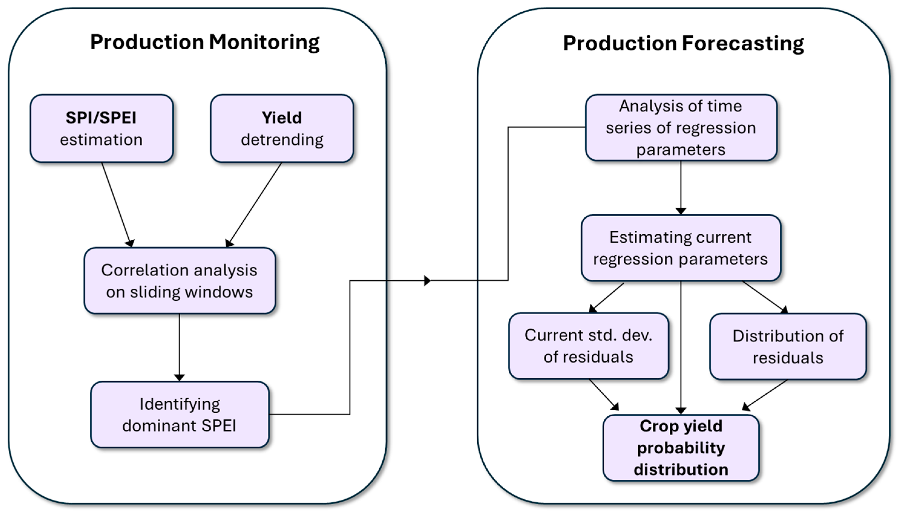
The methodology proposed in the present study is articulated in two main phases: (i) long-term monitoring and (ii) short-term forecasting (Figure 1). The monitoring phase uses as input time series of crop yield data and climatic indices (such as SPI or SPEI), each longer than 30 years. By means of a correlation analysis conducted on (minimum) thirty-year time windows sliding over the studied time interval, monitoring facilitates the identification of systematic temporal variations in the correlation of yield with specific climatic indices. Consequently, the dominant climatic index, i.e., the index that is becoming increasingly influential over time [11,12,13], is identified. The short-term forecasting phase takes this information as input to estimate the parameters of a reliable model describing the relationship between crop yield and the climatic indicator. The short-term forecasting provides as output the conditional probability distribution of crop yield, given an observed climatic index value. The long-term monitoring phase of analysis has been illustrated in detail by Guerriero et al. [12,13]. Nevertheless, the main steps of this phase of the analysis are summarized in the following sections for completeness and clarity.

2.2. Statistical Analysis of Climatic and Yield Data

The climatological analysis underpinning this study is based on datasets comprising daily and monthly time series of temperature and precipitation, along with crop production data. For instance, for the illustrative case study reported in this paper, climatic data were obtained from official publications of the Regional Hydrographic Service of Abruzzo at specific monitoring stations covering the period 1952–2014. Production data—annual time series of provincial cultivated area and total wheat production over the same period (allowing for the calculation of specific yield per hectare of land)—were retrieved from the Italian National Institute of Statistics (ISTAT) [11].

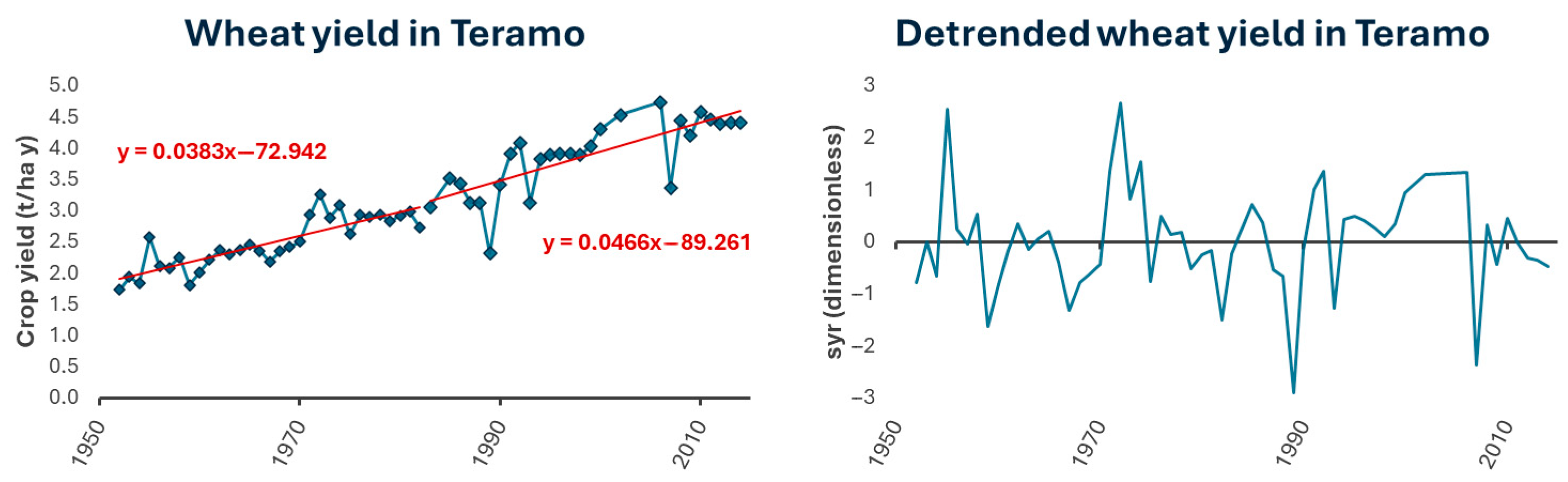
The statistical analysis phase aims at investigating the correlation between climatic indices and standardized detrended crop yield data. Detrending of yield values aims to isolate interannual fluctuations from a long-term trend, likely attributable to forms of climatic adaptation and the adoption of agronomic and technological solutions directed at enhancing crop production [11,12,13,30]. Detrending can be performed by considering, for each year, the residuals (r) derived from the difference between observed yield and that predicted by a linear regression model. Following the acquisition of the residual time series, standardized yield residuals (SYR) can be calculated as a standardized variable using the formula: SYR = (r − m)/s, where m and s denote the estimated mean and standard deviation of residuals, respectively.

Given our previous findings [12,13], which showed that SPI and SPEI provided comparable results in the study area—and that the 3-month SPEI (SPEI3) exhibited the strongest influence on yield—the present discussion will focus on the analysis of SPEI3 for conciseness. The choice of SPI and SPEI indices and their correlation with detrended yield values, for the studied crops and area, are discussed in detail by Guerriero et al. [11,12,13].

It is worth recalling that both SPI and SPEI are derived through a standardization process that accounts for the inherently asymmetric distribution of monthly precipitation, which is typically modeled using a Gamma distribution [26,28,29]. The tails of this distribution include rare events, characterized by exceptionally high or low precipitation values. Therefore, SPI and SPEI capture not only ordinary climatic fluctuations but also extreme events. More generally, in the absence of such a priori knowledge, the analysis could be extended to include all potentially relevant indices, whether monthly, quarterly, semi-annual, or others climatic variables.

2.3. Modeling the Yield–Drought Index Relation: Linear and Polynomial Regression

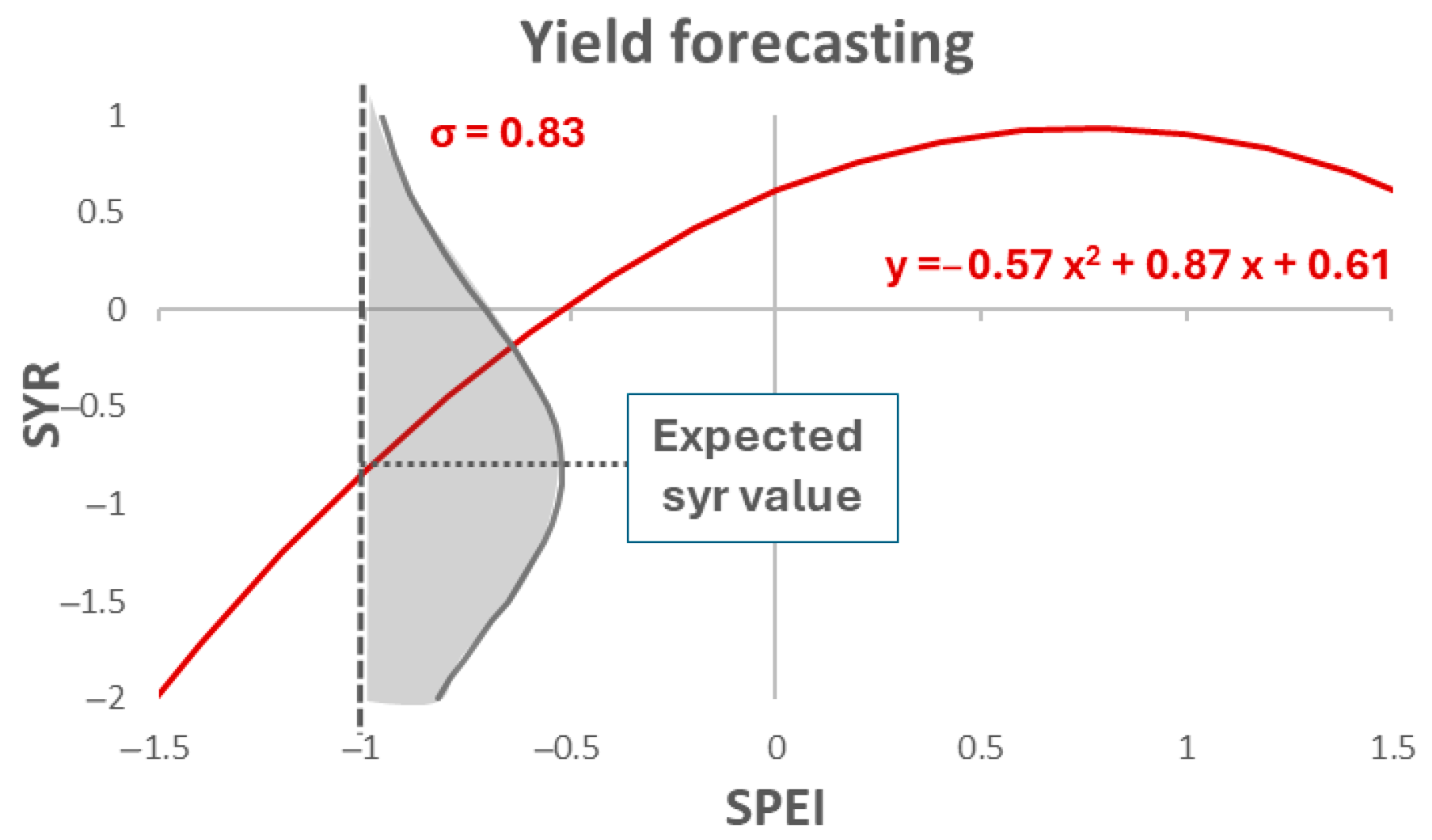
To characterize the relationship between SYR and drought indices, a commonly used regression model is a parabola (second-degree polynomial, Figure 2) exhibiting downward-sloping branches, reflecting the expectation that both severe drought and excessive wet conditions can limit crop productivity ([5] and references therein). Consequently, the vertex of the parabola is typically positioned around an optimal SPI or SPEI for crop production in a specific location; deviations from this optimum are associated with yield decline.

The linear model may be viewed as a simplified alternative to the more accurate polynomial model, offering certain advantages in terms of interpretability and ease of application [11,12]. The selection of the appropriate model to describe the SYR–SPEI relationship—whether linear or polynomial—will be based on criteria of statistical significance and method efficiency, as explained in detail in the next sections (Section 2.6, Section 3.1, Section 4). In any case, it is recommended for consistency to employ the same model during both the monitoring and forecasting phases.

2.4. Monitoring the Response of Production Systems to Climatic Fluctuations

The long-term monitoring phase of crop production involves regression analysis between the time series of SYR and climatic indices. This analysis is iterated across time windows of approximately thirty years in width, sliding through the whole analyzed period of observation. For instance, in the case study considered here, the initial time window covers 1952–1981, the subsequent one 1953–1982, and so forth. This approach generates time series of correlation coefficients and regression parameters for each considered index, enabling the evaluation of any systematic temporal variation. Furthermore, based on the observation of the correlation trends for the various analyzed indices, the dominant one (i.e., the index which is becoming the most impactful on crop yield) is identified.

2.5. Short-Term Yield Forecasting

According to a quadratic regression model, the relationship between SYR and the identified key climatic variable (here, SPEI3) can be described for each data point (individuated by the index j) as follows [31,32]:

SYR_j = y_j(SPEI3) + e_j(0, σ);

(1)

where e_j is a random variable (the noise) with a mean of zero and a finite standard deviation of σ, and y_j(SPEI3) represents the expected detrended yield, corresponding to the year j, defined by a second-degree polynomial:

y_j(SPEI3) = a ∙ SPEI3_j² + b ∙ SPEI3_j + c;

(2)

Here, a, b, and c are the parameters that characterize the polynomial relationship and are contingent upon the production system’s response to SPEI3 variations. In Equation (1), SYR pertains to the wheat harvest period, while SPEI3 represents the dominant index, which is generally estimated during a period preceding harvesting. This temporal separation can be leveraged for short-term forecasting purposes. For instance, if long-term monitoring confirms that the dominant index (for wheat cultivated in a specific area) is the SPEI3 in March, then registering this index in March would enable generating forecasts regarding the summer harvest.

Analogous to the monitoring phase, the regression analysis is also conducted over time windows spanning a minimum of thirty years, sliding across the entire study period. For each time window, the regression parameters of Equation (2) can be readily estimated using the ordinary least squares method. Once the value of the independent variable SPEI3 is known, the expected value y(SPEI3) can be calculated by means of Equation (2). Given that e_j is a random variable with a mean of zero and a standard deviation of σ (to be estimated), Equation (1) indicates that SYR (pertaining to the upcoming harvest) is a random variable with a mean equal to y and a standard deviation of σ. The probability distribution of this latter variable represents the conditional probability distribution of SYR given the observed value of SPEI3 (Figure 3).

Focusing, for the moment, on a single time window, once the parameters a, b, and c are estimated, the residuals e_j are calculated as the difference between the observed SYR value and the expected value y_j. The resulting series of residuals allows for the estimation of the standard deviation σ and the identification of the empirical cumulative distribution function [31] to determine the kind of probability distribution (Normal, Lognormal, etc.) that best approximates it. Once the form of the distribution and the standard deviation of the e_j values are known, the desired conditional probability distribution is fully determined.

At this point, this analysis can be extended from a single time window to the entire dataset to obtain more precise parameter estimates (due to the larger dataset). However, given the expectation that all parameters defining the desired conditional distribution (a, b, c, σ) may vary over time, it is not advisable to conduct the regression analysis on the entire dataset simultaneously. Instead, it is more appropriate to conduct the analysis on sequential (e.g., thirty-year, as in the case study) time windows (analogous to the monitoring phase; Section 3.2) to evaluate how these parameters evolve over time. This kind of analysis provides time series of parameters (a, b, c, σ), from which it is possible to estimate the current values. By linking each parameter estimate to the central year of its corresponding time window (e.g., 1966 for the 1952–1981 window), the current values of the parameters (a, b, c, σ) can be estimated by extrapolating the respective trendlines.

We highlight here that the parameter estimates presented in this study are derived from a non-standard analysis applied to a sixty-year dataset. Therefore, the statistics estimated for each thirty-year time window, including those related to statistical significance, should be interpreted as a preliminary result that is to be followed by a more robust analysis involving the whole sixty-year sample. For significance testing, we considered both the p-value [32] and the Akaike Information Criterion (AIC) [33], the latter being particularly useful for selecting the most appropriate regression model (in our case, linear or parabolic).

Since forecasting relies on the index currently exhibiting the highest correlation with yield, it is possible that significance statistics may produce spurious results for the earliest time windows (i.e., those beginning in the 1950s or 1960s), where the selected index may also have had a weak correlation with yield. Furthermore, it is important to note that estimation errors in the parameters a, b, c, and σ all contribute to the uncertainty in the predicted SYR value, which is the quantity of primary interest. Therefore, for forecasting purposes, it is particularly valuable to estimate the Root Mean Squared Error (RMSE) of the predicted SYR value, rather than the RMSE associated with individual parameter estimates for specific windows. This statistic can be effectively evaluated by replicating the estimation errors of SYR through the illustrated procedure, by means of Monte Carlo simulations, as described below.

2.6. Validation by Monte Carlo Simulations

A convenient approach to verify the performance of the proposed method involves conducting analyses on simulated datasets with known parameters. The estimates achieved can then be directly compared against the true parameter values.

The main aim of these simulations consists in replicating the forecasting capability achievable with our available sample—which, in the case study below, comprises 58 SYR and SPEI values recorded over approximately sixty years—by comparison of expected SYR value against the observed one, for the year immediately following the last in the series. By treating the sample of 58 values as a training set and the 59th value as a test set, Monte Carlo simulations offer the significant advantage of allowing the experiment to be replicated any number of times, thereby providing robust statistical insights.

Therefore, we performed a series of Monte Carlo simulations, generating synthetic datasets, each one consisting of 58 triplets of (SYR_k, SPEI_k, t_k) values. This simulation assumed linear trends for the parameters describing the parabolic SYR–SPEI relationship (Equation (2)), and for the standard deviation of the residuals, σ (assumed constant), and utilized likely fixed values for the parameters defining such trends. In these triplets, SYR_k and SPEI_k denote the SYR and SPEI values recorded in year t_k. In each simulation, a sample of triplets corresponding to 58 consecutive years served as a training set for forecasting; an additional triplet of simulated values for the 59th year was used as a test set to evaluate the difference between the observed SYR value from the predicted one.

The simulations were performed according to the following phases: fixed, plausible values were assigned to all trend parameters and to the standard deviation σ. Based on these values, for each t_k, a SPEI value (following a standard Normal distribution) was generated using random numbers. Furthermore, a deviation around the interpolating curve at time t_k was generated, following a Normal distribution with zero mean and standard deviation σ. Using the sample thus achieved, the parameters a, b, and c of the parabola describing the SYR–SPEI relationship (Equation (2)) for the year following the last in the series (i.e., for t₅₉) were estimated. A simulated SPEI₅₉ and SYR₅₉ value were then generated according to the same procedure. Based on the parameter estimates achieved from the training set and the SPEI₅₉ value, the expected SYR₅₉ value was estimated. Then, the difference between the simulated SYR₅₉ value and the predicted one was calculated. This process was repeated 1000 times, using the same parameters, thereby yielding 1000 values for the deviations of observed SYR from predicted SYR, for which the RMSE has been estimated.

Further cycles of 1000 analogous simulations were conducted using a simulated dataset where the three parameters in Equation (2) did not follow a linear trend but exhibited an irregular pattern, simulated by means of a simple autoregressive model.

3. Results

This section illustrates the application of the proposed methodology to the case study of wheat yield in the province of Teramo, Abruzzo region, preceded by a validation phase.

3.1. Validation

Monte Carlo simulations allowed us to thoroughly evaluate the forecasting method’s performance, both in predicting the next SYR value and estimating the various parameters defining the SYR–SPEI relationship. Additionally, these simulations enabled a comparison of the analysis method’s performance when employing a polynomial model versus a linear model to describe the SYR–SPEI relationship. Figure 4 shows an example of the estimated trend (dashed blue line) for the three simulated parameters (solid red line) according to a polynomial model for the SYR–SPEI relationship.

The simulation results for both models are summarized in

Table 1. Results of analysis involving data from Monte Carlo simulations in which polynomial parameters a, b and c, vary linearly over time.

	True Value	Linear Model	Polynomial Model
a	−0.738	0	−0.796
Standard dev. a	0	0	0.340
b	0.896	0.947	0.942
Standard dev. b	0	0.633	0.409
c	0.535	−0.163	0.575
Standard dev. c	0	0.421	0.444
σ	0.940	1.335	0.942
Standard dev. σ	0	0.384	0.254
Expected SYR uncertainty	0	1.233	0.743
RMSE (test set)	0	1.517	1.182

, where the obtained estimates are compared against their true values (those used to generate the simulations). For parameters a, b, c, and σ, we report the mean value and standard deviation from the 1000 simulations. The row labeled “Expected SYR Uncertainty” indicates the standard deviation of the observed deviation between the SYR value predicted for year t₅₉ (using the a, b, and c parameters estimated in each simulation) and the value calculated using the true parameter values. It is crucial to note that this value is not the SYR value at t₅₉ itself, but rather the value derived from the parabola describing the SYR–SPEI relationship, without the addition of stochastic fluctuation. The resulting standard deviation quantifies the uncertainty associated with parameter estimation error.

The value RMSE (test set) denotes the RMSE estimated for the deviations of SYR observed at t₅₉—including stochastic fluctuations—and that predicted. From these data, it is evident that the polynomial model exhibits less dispersion in the estimation of all parameters compared to the linear model, along with a lower RMSE value.

Figure 4b illustrates an example of estimating the trend of the three parameters a, b, and c, simulated using a simple autoregressive model. As an example, the equation for parameter a is:

a(t_k+1) = a(t_k) + N(m,s);

(3)

where N(m,s) is a Normal variable with constant mean m and standard deviation s, respectively. Parameters b and c are described by similar equations, with different values for m and s. For this model, five distinct determinations of the a, b, and c parameter trends were considered, all obtained with the same m and s values. For each determination, 1000 forecasting simulations were conducted, with the primary variation between simulations being the random fluctuations of SYR relative to the polynomial describing the SYR–SPEI relationship. In this specific context, forecasts were performed considering only the polynomial model. The results are presented in

Table 2. Results of analysis involving data from Monte Carlo simulations in which polynomial parameters a, b and c vary irregularly over time, according to an autoregressive model.

	SIMULATION 1			SIMULATION 2			SIMULATION 3			SIMULATION 4			SIMULATION 5
	True Value		Estimated	True Value		Estimated	True Value		Estimated	True Value		Estimated	True Value		Estimated
a	−0.627		−0.730	−0.362		−0.356	−0.933		−0.873	−0.484		−0.487	−0.736		−0.795
Standard dev. a			0.321			0.371			0.330			0.335			0.336
b	0.578		0.550	0.880		1.068	0.846		0.852	0.755		0.723	1.030		1.133
Standard dev. b			0.400			0.404			0.402			0.400			0.422
c	0.718		0.858	1.712		1.634	1.291		1.282	0.592		0.596	0.905		0.913
Standard dev. c			0.422			0.459			0.431			0.430			0.432
σ	0.940		0.921	0.940		1.033	0.940		0.942	0.940		0.944	0.940		0.951
Standard dev. σ			0.253			0.270			0.255			0.255			0.258
Expected SYR uncert.			0.747			0.823			0.748			0.872			0.648
RMSE (test set)			1.189			1.229			1.166			1.269			1.130

.

3.2. Long-Term Monitoring of Production

3.2.1. Analysis of Yield Time Series and Detrending

According to the available data, wheat production in the province of Teramo exhibits a yield with a substantially increasing trend over the period spanning 1952 to 2014 (Figure 5). Two yield sub-trends were calculated for two approximately thirty-year periods: 1952–1981 and 1982–2014. Yield residuals were computed relative to these sub-trends and subsequently standardized according to the methods illustrated in Section 3.1.

3.2.2. Time Series of Correlation Coefficients and Assessment of the Most Impactful SPEI Index

Figure 6 shows the correlation coefficients (coefficient of determination R²) between detrended yield and SPEI3 calculated on different months across sequential thirty-year time windows.

The figure reveals that the SPEI3 indices for the month of April generally exhibit an increasing influence on crop yield over time, exhibiting both the highest absolute value in the final period of observation and an overall increasing trend. Consequently, April SPEI3, identified as the most relevant index, is used as the basis for the short-term forecasting analysis.

3.3. Short-Term Forecasting of Production

3.3.1. Estimating the Current Regression Parameters

The regression analysis between SYR and April SPEI3, carried out over consecutive 30-year time windows, reveals significant temporal variability in the parameters of the second-order polynomial model, as shown in Figure 7, which presents the fitted polynomials functions for four time windows, each spaced approximately a decade apart.

For these same time windows, in addition to the parameters, further statistics were estimated for both the linear and polynomial models (

Table 3. Linear and quadratic regression models adjusted for describing the relation between Standardized Yield Residuals (SYR) and quarterly Standardized Precipitation Evapotranspiration Index (SPEI) of April in the Teramo province, Central Italy. Example of statistics estimated for four different time-windows, denoted as follows. (i) S.E.: Standard error of the estimate; (ii) p-value: Nominal significance level of the t-test for the null hypothesis that the parameter equals zero; (iii) RMSE: Squared root of the residual mean square; (iv) AIC: Akaike criterion for model selection.

Model	Parameter	Period	Estimate	S.E.	p-Value	R2	RMSE	AIC
Linear	Intercept	1952–1981	0.034	0.179	0.849	0.035	0.976	0.486
		1960–1990	−0.076	0.175	0.669	0.127	0.950	−1.136
		1970–2000	0.179	0.171	0.304	0.212	0.935	−2.099
		1980–2014	0.008	0.169	0.963	0.179	0.910	−3.741
	Slope	1952–1981	0.159	0.158	0.323	0.035	0.976	0.486
		1960–1990	0.314	0.156	0.054	0.127	0.950	−1.136
		1970–2000	0.472	0.172	0.011	0.212	0.935	−2.099
		1980–2014	0.474	0.192	0.020	0.179	0.910	−3.741
Polynomial	Intercept	1952–1981	0.231	0.282	0.419	0.063	0.979	1.586
		1960–1990	0.070	0.268	0.797	0.143	0.958	0.293
		1970–2000	0.440	0.248	0.087	0.267	0.918	−2.287
		1980–2014	0.325	0.219	0.149	0.296	0.858	−6.331
	Linear coefficient	1952–1981	0.148	0.159	0.362	0.063	0.979	1.586
		1960–1990	0.301	0.158	0.067	0.143	0.958	0.293
		1970–2000	0.514	0.171	0.006	0.267	0.918	−2.287
		1980–2014	0.532	0.183	0.007	0.296	0.858	−6.331
	Quadratic coefficient	1952–1981	−0.153	0.169	0.373	0.063	0.979	1.586
		1960–1990	−0.116	0.162	0.477	0.143	0.958	0.293
		1970–2000	−0.258	0.181	0.164	0.267	0.918	−2.287
		1980–2014	−0.398	0.189	0.044	0.296	0.858	−6.331

). Among these, those related to significance, such as the p-value and AIC, are particularly interesting. The p-value associated with the coefficient of the quadratic term decreases over time, reaching a value of 0.044, which currently indicates statistical significance. This is consistent with the fact that April SPEI3 showed a low and less significant correlation with SYR in the earlier period, while the increasing trend gives it high correlation values in the current period (Figure 6). The AIC statistics also provide similar results. It is recalled that, according to Akaike [33], between two alternative regression models (in this case, linear and polynomial), the one with the lower AIC value is preferable. The polynomial regression model presents the lowest AIC value for the two most recent time windows (1970–2000 and 1980–2014). These results are consistent with those obtained in the Monte Carlo-based validation (Table 1).

The time series of the three parameters associated with the polynomial regression (a, b, c) show clear trends (Figure 8). The figure displays these series along with their respective trendlines, which enable the estimation of the parameters for the year following the last in the series, which, in this case, is 2015.

3.3.2. Analysis of Residuals

The analysis of the residuals with respect to the regression curve, performed on sequential thirty-year time windows, provided a time series of the standard deviation values of the residuals e_j (Figure 8). The estimation of the residuals’ standard deviation accounted for the degrees of freedom inherent in the regression model, i.e., N-3 (where N is the sample size and 3 is the number of parameters of the regression model).

The trendline associated with this series enables the estimation of the standard deviation for the year following the final one in the dataset. In contrast to the parameters a, b, and c estimated above, the standard deviation of the residuals exhibited limited variability and a weak trend, with all values consistently falling within the 68% confidence interval of a constant average value (Figure 8), throughout the entire observation period.

Figure 9 shows the empirical probability distributions of the residuals computed for four time windows spaced at roughly ten-year intervals. The corresponding best-fit Normal distributions are overlaid in red. In all cases, the Normal distribution provides a reasonably accurate approximation of the observed empirical data.

3.3.3. An Example of a Short-Term Yield Forecast

A practical example is presented herein to demonstrate the practical application of the proposed yield forecasting procedure. The time series and associated trendlines reported in Figure 8 provided the following estimates for the parameters in the year 2015: a = −0.57, b = 0.87, c = 0.61, and σ = 0.83. Now, for illustrative purposes, let us assume that in the subsequent year, an April SPEI3 equal to −1 is recorded (indicated by a vertical dashed line in Figure 10). Using the polynomial regression function defined by the estimated parameters (a, b, c), the expected standardized yield residual (SYR) can be computed, resulting in a value of −0.82 (a value close to σ purely by coincidence). Consequently, the conditional probability distribution of SYR—highlighted by the shaded gray area in Figure 10—is a normal distribution with a mean of SYR∗ and a standard deviation of σ. This allows for straightforward probability calculations, using standard spreadsheet tools, to assess the likelihood of SYR exceeding or falling below any specified threshold of interest. For instance, the probability of SYR < −1.5, based on the derived distribution, is 21%. To determine the corresponding wheat yield associated with SYR = −1.5, the inverse of the standardization procedure described in Section 3.1 is applied. Referring to the yield trend over the period 1983–2014 (Figure 4), the expected yield for 2015 (y⁎) is estimated to be 4.64 tons/ha, with a standard deviation of the residuals around the trendline equal to s = 0.38 tons/ha. The yield threshold y corresponding to SYR = −1.5 is therefore calculated as: y = −1.5⋅s + y∗ = 4.06 tons/ha. Hence, the conditional probability that the expected yield will fall below 4.06 tons/ha, given an April SPEI3 of −1, is 21%.

4. Discussion

The validation of the presented method demonstrates that the polynomial model describing the SYR–SPEI relationship is definitively preferable to the linear one, as it yields estimates with lower uncertainty. This finding aligns with the statistical significance analysis conducted on both models across various thirty-year time windows (Table 3). For the polynomial model, the p-value associated with the coefficient of the second-degree term is below 5% in the most recent time window (i.e., 1980–2014), indicating statistical significance. Furthermore, the AIC statistic for the polynomial model is lower than that for the linear model in the two more recent time windows. This condition confirms the polynomial model’s preference over the linear one [33]. It should be reiterated, however, that the described significance analysis provides a preliminary result, as each statistic is estimated over a specific thirty-year time window, whereas the RMSE estimated via Monte Carlo simulation considers sixty-year samples analogous to the real-world data analyzed.

Moreover, it is crucial to note that the estimated RMSE provides a direct measure of the scattering of future SYR values relative to predicted ones. So, it truly represents the needed parameter for forecasting. Since the most effective forecasting method is one that provides the least uncertainty regarding the future SYR value, it is clear that the polynomial (parabolic) model is preferable as it yields the lowest test set RMSE.

The RMSE value differs from σ in Equation (1) because σ represents the intrinsic variability of the residual e_j, whereas RMSE incorporates, in addition to this variability, the estimation error on the parameters committed in each simulation. Specifically, if we denote by V the variance of the deviation of the expected SYR value from the true expected value (which would be obtained from Equation (1) if the exact values of parameters a, b, and c were known), then, assuming these uncertainties are stochastically independent, it is well established that RMSE² = V + σ² [31]. For the purpose of SYR forecasting, as illustrated in Figure 3, RMSE represents the standard deviation of the deviation between the observed SYR value and its predicted value. In other words, the SYR value of the next harvest is a Normal variable with a mean equal to the value determined by the parabolic SYR–SPEI relationship for the current year, and a standard deviation equal to RMSE. Consequently, Monte Carlo simulations, besides validating the method, can be integrated into the method itself as a phase for RMSE estimation. Should one wish to avoid Monte Carlo simulations for methodological simplicity, a rapid estimate can be obtained directly using the estimate of σ. However, it must be acknowledged that this estimate is less accurate than that obtained through Monte Carlo simulations and leads to an underestimation of the future SYR value’s variability.

By relying on the monitoring of appropriate climatic indices, the proposed short-term yield forecasting method can serve as an effective tool for both probabilistic estimation of agricultural production and related risk assessments. When integrated with price models proposed in previous studies [16,22,24], this approach can support the estimation of future price fluctuations of agricultural products, thereby enabling economic stakeholders along the production–consumption chain, as well as investors in financial markets, to perform informed risk analyses.

The methodology is scalable and adaptable across multiple spatial scales (from local to global) and with varying degrees of resolution (e.g., regional, provincial, or farm-level). However, the appropriate scale and resolution for analysis—particularly when applied to price forecasting—depend on the characteristics of the specific crop. For instance, in the case of local products, a provincial-level analysis, such as the one presented here, may be sufficient. Conversely, for crops traded on global markets, a broader, international-scale analysis is required. It is also worth noting that previous studies [11,12,13] have revealed significant variability in crop response trends even among neighboring provinces. As a result, the choice of the spatial resolution should be carefully considered, ideally targeting regions or countries that play a central role in the production of the crop under examination. This aspect could be the subject of future research.

In light of the potential applications outlined above, it is equally important to acknowledge the limitations inherent in the current implementation of the approach. The main one lies in the estimation of the trends for the parameters (a, b, c, σ), as shown in Figure 8. Specifically, each parameter is estimated over a moving thirty-year window. However, since these parameters likely vary within each three-decade span, the resulting estimates effectively represent averaged values. Additionally, the trendlines were derived using the ordinary least squares method, which assumes stochastic independence of residuals [31,32]—an assumption not satisfied in the case study presented. For example, the parameter ‘a’ estimated for the 1952–1981 and 1953–1982 windows is based on two datasets sharing 29 years in common. This overlap introduces dependencies that affect the trendline estimates and, consequently, the projection of current values (e.g., for 2015) used in the yield forecasting exercise. While the use of moving time windows undoubtedly provides more accurate insights than a single regression analysis over the entire period—allowing for the detection of temporal changes in correlation strength and other regression parameters, as well as a more refined estimation of their current values—it still involves a degree of approximation. The associated inaccuracies can introduce unknown estimation errors. Therefore, identifying more effective methods for estimating these trendlines constitutes an important direction for future research.

A further limitation in this study concerns the dataset employed in the illustrative case study, which covers the period from 1952 to 2014. This time span was selected to ensure data completeness and to minimize missing values in both climatic and yield data. Given that the aim of this application was primarily to demonstrate the methodology, some simplifications were introduced—such as using aggregated wheat production without distinguishing between durum and soft wheat—despite potential differences in their yield performance and cultivated areas over time. While the detrending process mitigated some of these effects, the use of more recent and disaggregated data could support future studies in achieving more detailed and robust assessments for the investigated area.

Finally, a further enhancement to the analysis could involve a multivariate approach, incorporating additional variables beyond SPEI that potentially impact yield, such as temperature-related indices, CO₂ concentration, and others. In this type of analysis, a multivariate linear regression model can offer valuable first-approximation insights into combinations of climatic variables that most significantly influence yield. However, this approach has some limitations: a linear model assumes the joint effect of two variables is merely the sum of their individual effects. In reality, there may be situations where only the combined effect of two events (e.g., both covariates exceeding a certain threshold) has a significant impact on yield, while the occurrence of a single event (only one variable exceeding a threshold) shows no appreciable impact. For these reasons, the selection of the appropriate model for a multivariate analysis requires careful consideration. Such an investigation falls outside the scope of this article but represents an interesting avenue for future research.

5. Conclusions

This study proposed a statistical methodology for short-term crop yield forecasting based on the monitoring of climatic indices. The method has been validated and integrated by a Monte Carlo approach and illustrated through the case study of wheat production in the province of Teramo (central Italy). The approach complements a long-term monitoring framework previously introduced by the authors. The overall analytical workflow can be divided into two sequential phases: (i) long-term monitoring and (ii) short-term forecasting. The monitoring phase requires time series exceeding 30 years for both crop yield and climatic indices. Through a correlation analysis applied to moving time windows, this phase identifies the dominant climatic index (i.e., the index exerting the greatest influence on crop yields). The forecasting phase uses this information to estimate the current parameters of the statistical model describing the relationship between yield and the selected climatic index. It then provides the conditional probability distribution of yield, given the observed current value of that index, thus supporting timely decision-making processes in the agricultural sector and enabling more informed risk assessments by both producers and all relevant stakeholders.