More Is Still Not Enough—What Is Necessary and Sufficient for Happiness?

Abstract

Happiness is defined as well-being and contentment with life. The growing imperative to evaluate well-being beyond economic growth alone has led to the formulation of holistic indices that better reflect quality of life and sustainable development goals. This has resulted in the emergence of the Happiness Score (HS), which adopts a more holistic and human-centred perspective on development and well-being. The present study takes the Happiness Score as a basis for the identification of some of the main determinants of happiness in an empirical and data-driven perspective. To this end, data from 145 countries was analysed, using statistical methodologies such as Generalised Linear Models (GLM), Principal Component Analysis (PCA), fuzzy set Qualitative Comparison Analysis (fsQCA) and the decision tree machine learning approach. A range of indices were considered to translate the reality of countries in different socio-economic dimensions, the level of development of each country, and the continent to which it belongs. The African continent demonstrates substantial disparities across virtually all variables and is frequently associated with the most unfavourable values for each index. The indicators that exerted the most profound influence on happiness were identified as the freedom to make life choices, literacy rate, and Gross Domestic Product (GDP) per capita. These results inform policy strategies aligned with sustainable development, emphasising that enhancing happiness requires multidimensional action beyond economic indicators—particularly in low- and middle-income countries.

1. Introduction

Measuring happiness and well-being goes back to various philosophical and economic traditions. Philosophers such as Aristotle discussed the concept of eudaimonia, which refers to a well-lived and prosperous life, while 20th-century economists began to recognise the limitations of traditional economic indicators. One of the first and most notable efforts to measure national happiness was made by the Kingdom of Bhutan in the 1970s. Bhutan’s fourth king, Jigme Singye Wangchuck, introduced the concept of Gross Domestic Happiness (GNH), proposing that development should be measured by the general happiness and well-being of the population, not just by economic growth. GNH covers nine domains: standard of living, health, education, cultural diversity and resilience, good governance, community vitality, ecological resilience, use of time, and psychological well-being. Inspired by Bhutan, other countries have tried to measure happiness and well-being. In 2012, the United Nations launched the first World Happiness Report, which measures happiness at a global level. This report uses data from global surveys and considers factors such as income, life expectancy, social support, freedom to make life choices, generosity, and perception of corruption. Since then, various countries and organisations have adopted and adapted methodologies to measure happiness and well-being. Governments, Non-Governmental Organizations (NGOs), and academic institutions continue to explore ways of integrating these metrics into public policies and development strategies. Measuring happiness generally includes surveys and questionnaires assessing life satisfaction, positive and negative emotions, and other indicators of subjective well-being. The Happiness Index emerged as a response to the limitations of traditional economic indicators, incorporating a more holistic vision. In the context of the UN Sustainable Development Goals (SDGs), particularly Goal 3 (Good Health and Well-being) and Goal 16 (Peace, Justice and Strong Institutions), measuring happiness and well-being has become a critical aspect of evaluating sustainable development progress.

The ‘Happiness Score’ used in the World Happiness Report is obtained from data from surveys by the Gallup World Poll. The creation of this index involves several stages: the implementation of a global survey covering a wide range of topics; the use of a self-assessment scale known as the ‘Cantril Ladder’, which is a figurative representation of life satisfaction ranging from 0 (the worst possible life) to 10 (the best possible life), on which respondents are asked to place themselves; the calculation of key components (GDP per capita, social support, healthy life expectancy, freedom to make life choices, generosity, and perceptions of corruption); the application of a regression model incorporating these components; and finally, the aggregation of the results. Despite its single-item format, the Cantril Ladder-based score has demonstrated validity in large-scale international studies and remains a reliable benchmark for cross-national happiness comparisons.

In 2021, the World Happiness Report concluded that Finland is the happiest country in the world. This index analysed 149 countries, specifically considering performance in six categories: gross domestic product per capita, social support, healthy life expectancy, freedom to make life choices, generosity of the general population, and perceptions of levels of internal and external corruption.

Over the years, happiness has increasingly become a recurring theme that is worth analysing [1]. Various studies have been carried out to understand the indicators with which happiness can be correlated, for various countries. The correlation of happiness with levels of corruption and GDP per capita are some of the most frequent conclusions. High levels of corruption are one of the main determinants of lower levels of happiness and satisfaction. High GDP per capita is also generally associated with high happiness. In addition to these categories, there are certainly many others that can influence the happiness of countries. This paper aims to identify the main determinants of happiness in countries, considering macroeconomic variables, social variables, crime levels, literacy levels, levels of innovation, and access to healthcare, among others. The aim is to understand how each of these variables behaves concerning happiness, as well as whether the continent of each country influences this relationship.

Some studies on this subject, including Jaswal et al. [2], and Li and An [3], have opted for exploratory data analysis and regression modelling. In this paper we will explore and evaluate the necessary and/or sufficient conditions for happiness, using diverse and complementary statistical approaches. To understand which continents differ on the various variables, multiple comparison tests will be carried out using parametric and non-parametric hypothesis tests. In addition to all the tests and models, the analysis of descriptive statistics graphs will be essential to corroborate all the conclusions drawn and to add information.

The present study makes two contributions: firstly, it explores new variables as potential drivers for happiness, namely the literacy rate, the crime rate, the innovation rate, and doctors per capita; secondly, it uses, besides the linear models, the fsQCA (fuzzy set qualitative comparative analysis) and decision tree machine learning approaches. The study employs these methodologies to analyse happiness, its necessary and/or sufficient conditions, and to evaluate the impact of each variable in a global context. The study further compares, for validation purposes, results obtained using regression models, factor analysis, fsQCA and decision tree approaches. In this context, relationships are captured globally, i.e., in a linear and non-linear way, allowing for a more in-depth analysis of the true determinants of happiness.

This work is structured as follows. First, a brief literature review is presented. Next, the data and methods are presented, including the sources and description of the database and the statistical inference, regression models, fsQCA and decision tree approaches. Later, in the results section, various models and hypothesis tests are used to achieve the desired objectives. Finally, the discussion of results and conclusions are presented.

2. Literature Review

Happiness is defined as well-being and satisfaction with life [4]. The growing concern to measure the well-being of populations beyond traditional economic indicators has led to the development of new indices that consider broader aspects of quality of life [5]. This development has resulted in the conception of the Happiness Score (HS), which adopts a more holistic and human-centred perspective on development and well-being [6]. In recent years, interest in the study of the happiness index and its determinants has been growing. The most common approach is to use statistical methods to try to determine the factors that contribute most to happiness. Several authors chose to use data from the World Happiness Report for more than 100 countries [3,7,8].

To approach the subject of happiness, various studies chose to carry out a statistical analysis of the data, starting with an exploratory data analysis, estimating regressions, and analysing models and confidence intervals. Several factors can contribute to happiness levels, such as GDP per capita, healthy life expectancy, social freedom, family, trust, and generosity, according to data from the Gallup World Poll. Some researchers also highlight elements related to the physical conditions that shape living conditions such as architectural solutions [9,10] or the more difficult to grasp elements that allow placemaking, where the community is bound to the place [11]. Despite their contribution, these may not represent the full set of factors that do so. The fact that society is constantly changing at a rapid pace means that measuring happiness requires consistency and innovation [2].

It is common to associate a lack of happiness with high levels of corruption in a country. Studies have been carried out to study the impact of corruption on subjective well-being [3,12]. Applying multiple linear regressions, it was possible to conclude that an increase in corruption by a government causes a decrease in the national average of well-being. The significant effect of corruption is only noticeable in democratic or high-income countries [3]. A country’s corruption lowers national income and institutional trust, which in turn lowers subjective well-being. The detrimental effect of corruption is more evident in Western countries than in non-Western countries [12].

According to López-Ruiz et al. [13], several factors positively affect the happiness of the population, in the case of Spanish society, these are the family situation, trust in the close circle and neighbours, a less polluted environment, culture, sports, safety in the place of residence, and the financial and employment situation. The COVID-19 pandemic harmed Spanish citizens’ quality of life and, therefore, their happiness. Although negative, its impact was not significant, and the authors concluded that a long-term analysis would be necessary to realise its true significance. To investigate the determinants of average satisfaction with life, the percentage of prosperity and suffering of people, and the negative and positive effects of this; with panel data models, it has been possible to understand what influences happiness in different countries over several years [7,14]. By using large international samples of individuals surveyed, it was possible to simultaneously identify the determinants of well-being at an individual and societal level. Using a variety of methodologies, direct and indirect correlations were found between social capital and well-being [14].

It is important to emphasise the distinction that still exists today in terms of development. This issue also ends up influencing the level of satisfaction and happiness. Corruption is an example of this since it is negatively related to the happiness index, especially in countries with greater wealth. Furthermore, the size of the GDP effect is smaller in more advanced economies [7]. As well as being influenced by various factors, happiness is also influenced by others, such as GDP per capita. Using the Granger causality test, Lee and Goh [8] concluded that happiness stimulates GDP per capita, with the positive effect of happiness on GDP per capita in developed countries being around four times greater than in developing countries.

Pereira et al. [15], using fsQCA, find that high national income, income equality, high-quality institutions, and each of the cultural dimensions are not necessary conditions for high subjective well-being (SWB). However, high power distance and low individualism are necessary conditions to achieve low SWB. Sedeh and Caiazza [16] implemented (fsQCA), to scrutinise the collective impact of entrepreneurial endeavours, institutional structures, and income equality on SWB. The fsQCA methodology was applied by Wu and Zhou [17] to analyse the configuration combination of psychological need satisfaction to improve the well-being of temporary workers in China. It was found that temporary workers pay more attention to whether respect recognition and career planning are met. Cheng and Xu [18] investigated the combination of causal and asymmetric relationships between benefits from touristic sharing and residents’ SWB in the Chinese region.

Machine learning methods based on decision trees were also used to identify factors influencing a community’s sense of happiness. Akanbi et al. [19], based on data from 156 countries, indicated that the best-fitting model is XGBoost, according to which GDP per capita, social support, healthy life expectancy, and freedom to make life choices (in that order) have the greatest impact on happiness. Similar results for the same type of models were obtained by Jannani at al. [20]. A study utilising a range of machine learning models (based on decision trees, regression or neural networks) indicated that GDP per capita emerged as the primary indicator, while social support and health expectancy were also identified as key factors both before and following the pandemic [21]. However, during the pandemic, social support was identified as the most significant indicator, followed by healthy life expectancy, and GDP per capita. This shift can be attributed to the pivotal role of social support in coping with the challenges posed by the pandemic.

To summarise the preceding discussion, it can be posited that, according to Jaswal et al. [2], happiness is predominantly influenced by social freedom and family. Conversely, Araki [7] underscores gross domestic product and corruption as the primary determinants of happiness. Other authors have highlighted the impact of corruption on happiness, including Li and An [3], and Tay et al. [12]. Conversely, Lee and Goh [8] adopted a different approach, concluding that GDP per capita is impacted by happiness.

Overall, when comparing the articles analysed, the influence of GDP per capita and corruption on happiness is clear. However, there are many other factors to consider when analysing happiness. The literacy rate, the crime rate, the innovation rate, and doctors per capita are some of the variables that will be studied in this work and that were not covered in the studies mentioned above. Given the literature review, this work aims to study the determinants of happiness for the year 2022. The aim is to study the impact of the following indicators on happiness: Corruption Perceptions Index, Crime Index, GDP per capita, social support, healthy life expectancy, freedom to make life choices, generosity, Human Development Index, literacy rate, doctors per capita, Global Innovation Index, unemployment rate, mortality rate due to road accidents, Gini coefficient. In other words, ‘Of the variables under study, which have a significant impact on the Happiness Index?’

3. Data and Methods

3.1. Data

To analyse happiness and identify its determinants, data were collected on various indices and rates that are correlated with happiness. The selection of variables in this study was based on previous empirical research on the determinants of happiness and quality of life (e.g., [22]). Key variables, including GDP per capita, social support, healthy life expectancy, generosity, freedom to make life choices, and perceptions of corruption, have been extensively examined in prior studies [7], and are therefore also incorporated into the present analysis. While some indicators may conceptually overlap, for instance, the Human Development Index (HDI) and literacy rate, their inclusion enables the evaluation of each dimension’s unique contribution across different analytical frameworks, such as Principal Component Analysis (PCA) and Fuzzy-Set Qualitative Comparative Analysis (fsQCA).

The database for this study consists of data from 145 countries (Table S1) for the year 2022. Data was collected for 15 quantitative variables and 2 qualitative variables (Continents and Development). Data were collected from reputable international sources, including the Gallup World Poll, World Bank, UNDP, and Transparency International (Table S2). The selection of the countries under study was based on the availability of information for the variables considered. It was also ensured that all continents were represented, and that there was variety in terms of the level of development and size of the country. As this is a cross-sectional study, the findings are associative in nature and not intended to imply causality. For all the analysis, we used R software, version 4.3.3. A significance level of 5% (α = 0.05) was used for the statistical tests.

3.2. Statistical Inference and Regression Models

To compare means between continents, a one-way analysis of variance (ANOVA) was used. The one-factor ANOVA model was applied to check for significant differences between the continents. This model is used when there is a categorical independent variable (factor) with levels and a continuous dependent variable. The model’s assumptions must be verified, i.e., the normality of the residuals and the homoscedasticity of the variances. In other words, the residuals of the model must follow a normal distribution and there must be homogeneity of variances between groups; the variances must not differ significantly.

To compare the averages between the countries’ levels of development, a t-test was carried out. This test requires the normality and homogeneity of the samples to be verified. To test the normality of the residuals, the Shapiro–Wilk test was carried out and the QQ-plot was analysed. The homogeneity of the variances was checked by Levene’s test and by looking at the graph of the residuals as a function of the adjusted values. Concerning comparing means between continents, if the residuals are normal, the Tukey method will be used to carry out the multiple comparisons. If normality is not verified, a non-parametric alternative to ANOVA will be applied, the Kruskal–Wallis test, and multiple comparisons will be carried out using Dunn’s test. On the other hand, if homoscedasticity is not verified too, a non-parametric alternative will be used, the Games–Howell test. When comparing means between levels of development, if the residuals are not normal, the Wilcoxon–Mann–Whitney test should be used. If normality and homoscedasticity are verified, the test to be used is Student’s t-test. If, on the other hand, normality is verified but homoscedasticity is not, the Welch test will be used.

After analysing the behaviour of the variables, it is time to move on to estimating models to define exactly which factors determine happiness. The Multiple Linear Regression model aims to understand the relationship between a dependent variable (in this case the Happiness Index) and several explanatory variables, making it possible to infer causality in cases where simple regression analysis would be misleading [23].

The model was first defined, and its assumptions were tested. The model’s residuals were standardised, the linearity of the model was checked, the normality of the residuals was tested, and the Breusch–Pagan test was used to test the homogeneity of the variances. The RESET test (model specification test) was carried out, and it was concluded that the model was correctly specified. Finally, the presence of outliers and influential observations were also tested. An influential observation was found to be influencing the significance of the model and the Unemployment Rate variable. It was possible to identify it and realise that it was Botswana. The adjustment was carried out without this country.

Multiple Linear Regression models were estimated, and, when variables were removed, it was checked in each pass whether the coefficients varied greatly. If this variation proved to be significant (>35%), the variable could not be removed from the model. A Generalised Linear Mixed Model was fitted to see if including a correlation structure considering continents as a random factor is important for the level of happiness. Criteria were used to compare this model to the previously estimated model. The AIC (Akaike Information Criterion) and BIC (Bayesian Information Criterion) allow us to determine which model best fits the data, with lower AIC and BIC values meaning a better model.

Finally, factor analysis was also considered. This technique aims to reduce the dimensionality of the data by grouping correlated variables into factors or components. By using a model with orthogonal components, it is assumed that these components are independent of each other. Cronbach’s alpha and the KMO index were used to measure the quality of the factor analysis. Cronbach’s alpha measures how well the variables are related to each other, and KMO assesses whether the model is adequately adjusted to the data. Spearman’s correlation coefficient was also calculated, which is a non-parametric measure that allows us to see whether the new variable created correlates with the variables removed from the model

3.3. Fuzzy-Set Qualitative Comparative Analysis (fsQCA)

FsQCA is a method developed by Charles Ragin [24,25], rooted in set theory, that enables the identification of causal configurations leading to an outcome of interest. It is widely used in social sciences and management studies to analyse complex causality, particularly in cases where multiple pathways may lead to the same result. Unlike traditional regression analysis, which assumes linear and additive relationships between independent and dependent variables, fsQCA examines the combinatory effects of conditions through Boolean algebra and fuzzy-set logic. One of the fundamental distinctions between fsQCA and linear regression lies in their epistemological assumptions. While regression analysis estimates the net effect of independent variables on a dependent variable under the assumption of linearity, fsQCA focuses on identifying necessary and sufficient conditions within a given dataset. Moreover, fsQCA allows for equifinality-the possibility that multiple configurations of conditions may produce the same outcome—whereas regression models tend to emphasise a single explanatory path. It also accommodates non-linearity and interactions more explicitly, providing a nuanced understanding of causal complexity that regression models often overlook. By assigning membership scores to cases on a continuous scale from 0 to 1, fsQCA enables researchers to analyse degrees of membership rather than relying on strict binary classifications. This approach enhances analytical precision and allows for a more refined exploration of causal relationships.

The process consists of several key steps:

• Case and condition selection—identify the outcome variable (dependent variable) and causal conditions (independent variables).
• Calibration of data—converting raw numerical data into fuzzy-set membership scores ranging from 0 to 1. Here, the classical percentile method was utilised, employing the thresholds: 0.05, 0.5, and 0.95. The variable Developing was transformed into a dummy variable (0 = Developing, 1 = Developed) and did not undergo calibration. To prevent cases with membership scores of 0.5 from being excluded from the analysis, we added a small constant (+0.001) to all scores below 1 [26].
• Constructing the truth table—generating a table representing all possible combinations of causal conditions and assigning rows based on their fuzzy-set membership scores. Here, the consistency threshold equals 0.8 to determine which configurations are reliably associated with the outcome used.
• Logical minimisation—apply the algorithm, here Consistency Cubes [27], to simplify complex causal patterns.
• Interpretation of the obtained solution (here, parsimonious) configuration.

3.4. Machine Learning Decision Tree Approach

The Random Forest (RF) model is an ensemble learning method composed of multiple decision trees. Each tree is trained on a randomly selected bootstrap sample of the dataset (sampling with replacement). At each split, a random subset of predictors is considered, reducing overfitting and enhancing model robustness. The final prediction is obtained by aggregating the outputs of all trees, typically through averaging (for regression) or majority voting (for classification). This method, which integrates bagging (Bootstrap Aggregating) and random feature selection, has been shown to improve predictive performance compared to standalone decision trees and other machine learning models [28]. In this study, all available predictors were used, and their importance was assessed using %IncMSE (Percent Increase in Mean Squared Error). This metric evaluates how much the model’s error increases when a given variable’s values are randomly shuffled. A significant increase in MSE indicates a crucial predictor, while a negligible change suggests a less influential variable.

XGBoost (Extreme Gradient Boosting) is a gradient boosting algorithm that sequentially constructs an ensemble of decision trees, where each new tree corrects the residual errors of the previous ones. Unlike RF, which builds trees independently, XGBoost optimises tree structure iteratively, prioritising difficult-to-predict instances to improve accuracy. To prevent overfitting and enhance generalisation, XGBoost incorporates L1 (Lasso) and L2 (Ridge) regularisation. Additionally, it introduces several computational improvements, such as tree pruning, parallel processing, and a weighted quantile sketch algorithm, making it highly efficient for large datasets [29]. These optimizations have contributed to XGBoost’s widespread adoption as one of the most effective machine learning algorithms for structured data task

4. Results and Discussion

Once the literature review has been carried out and the methods and tests to be used have been described, the results will be analysed. Exploratory analysis and data visualisation will be covered, as well as comparing averages and studying various models to arrive at a final model.

4.1. Exploratory Analysis and Data Visualisation

We first visualised the data in an exploratory analysis, looking for relevant information based on the distribution of each variable, either separately or grouped by continent or level of development. Measures of localisation, dispersion, and asymmetry were calculated for all these variables, as they are fundamental measures for describing the main characteristics of the data (

Table 1. Descriptives for quantitative variables.

Variable	Descriptives
	Max	Min	Mean	Median	SD	CV	Skew.
Happiness score	7.82	2.40	5.55	5.58	1.09	19.64	−0.25
Corruption Perceptions Index	90.00	14.00	43.9	38.00	18.77	42.75	0.72
Crime index	83.60	12.66	45.83	46.50	14.77	32.18	0.07
GDP per capita	2.20	0.00	1.41	1.44	0.42	29.96	−0.44
Social support	1.32	0.00	0.91	0.96	0.28	31.03	−0.86
Healthy life expectancy	0.94	0.00	0.58	0.62	0.18	30.09	−0.58
Freedom to make life choices	0.74	0.00	0.52	0.55	0.15	28.30	−0.83
Generosity	0.47	0.00	0.15	0.13	0.08	56.32	0.95
HDI	0.96	0.39	0.74	0.76	0.15	20.72	−0.37
Literacy rate	100.00	27.28	87.95	95.64	16.67	18.95	−1.83
Doctors per capita	70.60	0.30	21.94	21.60	17.81	81.09	0.51
Innovation index	64.60	6.00	29.56	27.90	14.63	49.49	0.46
Unemployment rate	28.84	0.23	6.96	5.07	5.48	78.65	1.72
Road traffic accidents death rate	67.23	1.69	19.46	15.09	15.18	77.99	0.93
Gini coefficient	0.63	0.23	0.37	0.35	0.08	20.73	0.78

).

The variables with the highest standard deviation are the Corruption Perceptions Index and the Doctors per capita. The coefficient of variation (CV) is the ratio between the standard deviation and the mean, in percentage. The higher the value of the coefficient of variation, the greater the variability of the data to the average. The variables Doctors per capita, Unemployment rate, and Road traffic accidents death rate have a high coefficient of variation (close to 80%), so the data is more dispersed around the mean. Skewness measures the symmetry of the data distribution. A value of zero indicates a perfectly symmetrical distribution. The higher the absolute value of the asymmetry, the more pronounced the asymmetry of the distribution. The variables are fairly symmetrical, only in two cases does the asymmetry exceed the absolute value of 1.

The variable Unemployment rate was also eliminated from the following analyses due to its ‘random’ nature. This variable refers to the number of unemployed people of working age, registered with a specific institution, who are available for work and have taken specific measures to find work. It was found that in some countries, the unemployment rate figures were not logical, for example, Nigeria (0.57%) or Moldova (0.9%). These low figures may be indicative of the fact that a significant proportion of the unemployed population in these countries is not registered, rather than suggesting a near-absence of unemployment. The histogram for the Happiness Score variable (Figure S1) is symmetrical and shows a leptokurtic distribution. The remaining variables are characterised by diverse distributions, encompassing both symmetrical and close-to-normal types, as well as asymmetrical configurations. European countries have the highest levels of happiness and social support (Figure 1). African countries, in addition to having the least social support compared to any other continent, are also the least happy countries, except for some Asian countries. The highest crime figures are mainly in Africa, but also in America and in some cases in Asia.

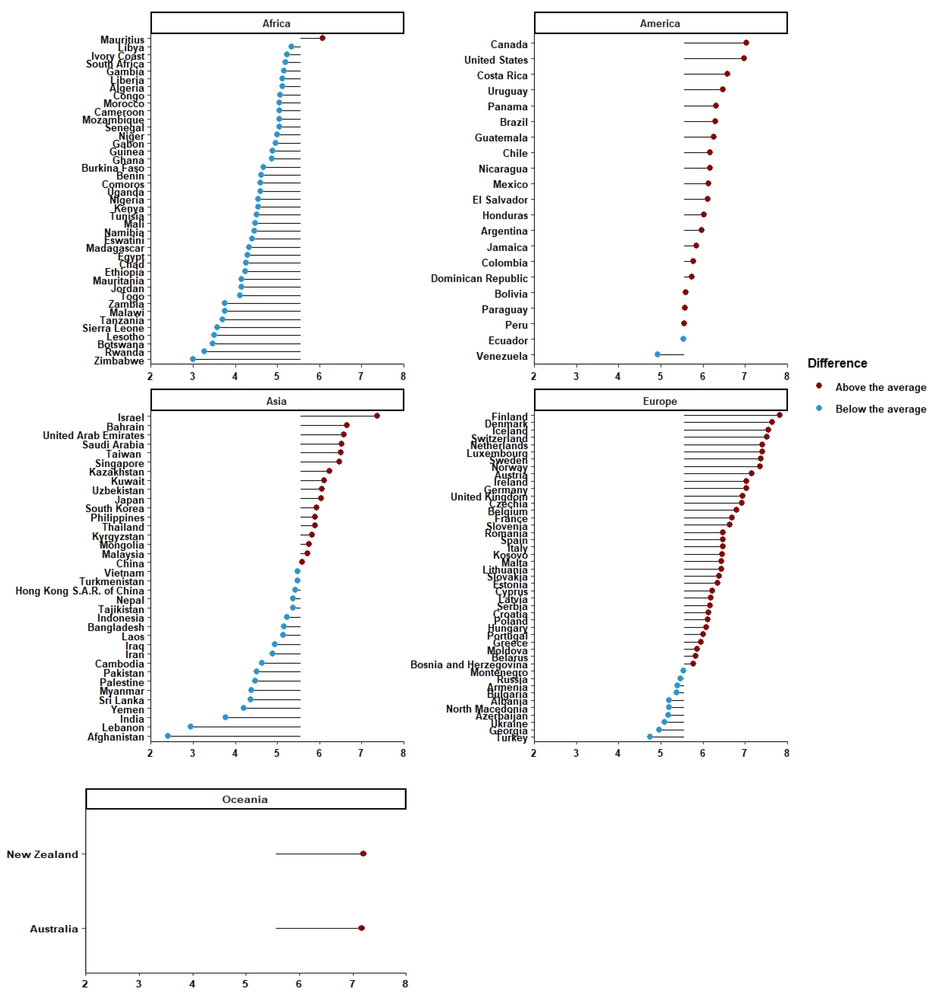
The differences in the global average Happiness Index for countries, separated by continent, are presented in Figure 2. When there are lines on the left-hand side (with the blue circle) it means that, for a country on a certain continent, the happiness index values are below average (of all countries), while when there are lines on the right side (with the red circle) the values are above average. The African continent stands out in the negative: only Mauritius has a happiness index above average. In both America and Europe, most countries have an above-average happiness index. There are differences in the countries’ Corruption Perceptions Index concerning the global average, broken down by continent (Figure S2). The lower a country’s Corruption Perceptions Index, the more corrupt it is, so in Africa, we can see that in most countries, this index is below average. Also, in America and Asia, from this graph, we can conclude that most countries are characterised by high levels of corruption. There are also observed differences between the countries’ Freedom to Make Life Choices and the global average, broken down by continent (Figure S3). Europe stands out because a large proportion of European countries have below-average values for freedom to make life choices.

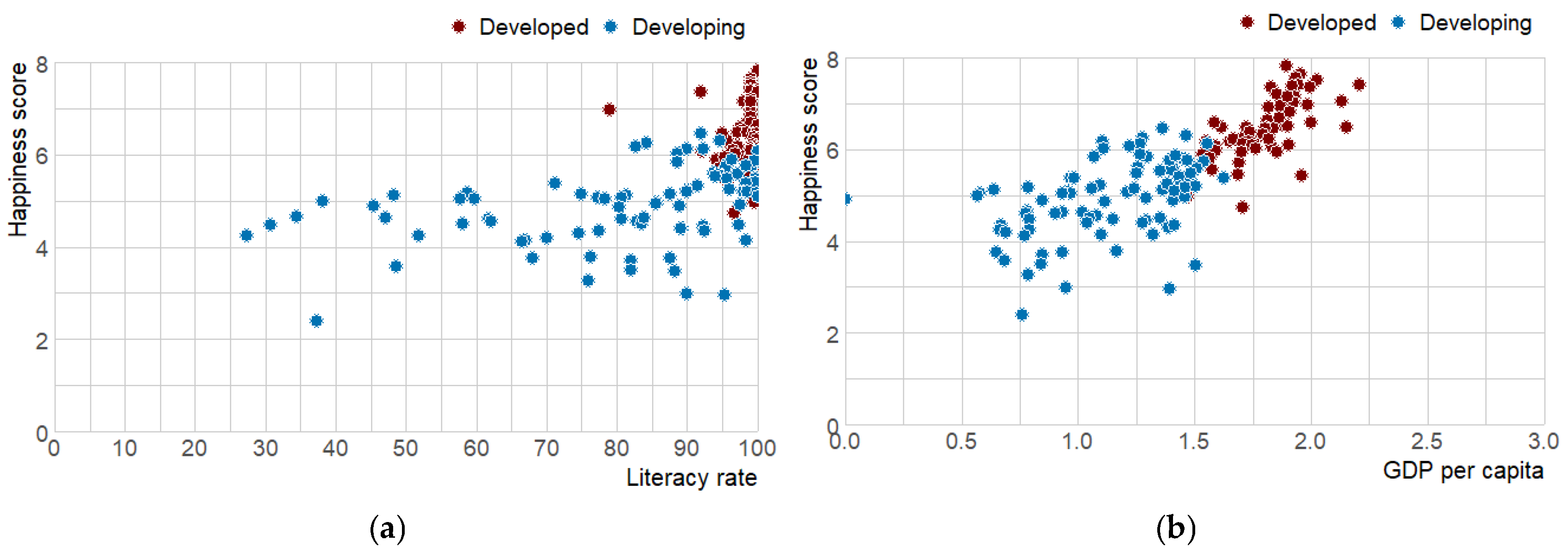
With regard to the scatter plot by the level of development of the happiness index as a function of GDP per capita (Figure 3a), it is evident that developed countries are approaching a higher happiness index, accompanied by a higher GDP. For developing countries, lower GDP values are associated with lower happiness values. Figure 3b highlights the fact that practically all developed countries have a literacy rate equal to or very close to 100. It is also in these same countries that the happiness index is highest.

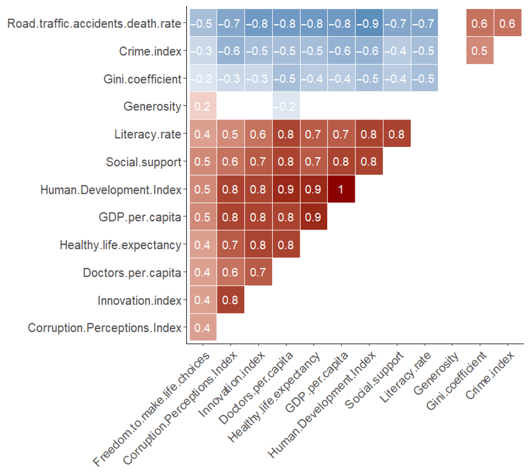
A correlogram between all the indicators (Figure 4) shows a high correlation between the Human Development Index and GDP per capita variables, the GDP per capita and Healthy life expectancy variables, the Human Development Index and Road traffic accident death rate variables, among others. The high level of correlation between variables should be considered as a potential sign of multicollinearity in regression models. In this sense, since the Human Development Index and GDP per capita variables correlate 1 (very high), they cannot both be included in the models to be estimated. Thus, the Human Development Index variable will not be included in the Linear Regression Models estimated later, because it is also strongly correlated (>0.8) with seven other quantitative variables. Removing it not only solves the problem of correlation with GDP per capita, but also solves this problem with other variables, thus avoiding future problems of multicollinearity.

4.2. Inference Analysis

Before applying regression models, it is necessary to understand whether there are significant differences between continents and levels of development for the variables under study. To this end, multiple comparison tests were carried out. The Continents variable is made up of five levels (Africa, America, Asia, Europe, and Oceania: Australia and New Zealand), and

Table 2. Differences between levels of development by indicator. Legend: (a) Student’s t-test; (b) Welch test; (c) Wilcoxon–Mann–Whitney test.

${HappinessScore }^{\left(a\right)}$			${CPI}^{\left(b\right)}$
	M ± sd	Developing		M ± sd	Developing
Developed	6.49 ± 0.65	<0.0001	Developed	61.03 ± 16.11	<0.0001
Developing	4.91 ± 0.83		Developing	32.15 ± 8.74
${Crimeindex}^{\left(a\right)}$			${GDP }^{\left(c\right)}$
Developed	36.39 ± 11.52	<0.0001	Developed	1.81 ± 0.16	<0.0001
Developing	52.44 ± 13.15		Developing	1.13 ± 0.31
${Socialsuport}^{\left(c\right)}$			${Healthylifeexpectancy }^{\left(b\right)}$
Developed	1.12 ± 0.12	<0.0001	Developed	0.73 ± 0.08	<0.0001
Developing	0.76 ± 0.26		Developing	0.48 ± 0.15
${Freedomtomakelifechoices }^{\left(c\right)}$			${Generosity}^{\left(c\right)}$
Developed	0.58 ± 0.12	<0.0001	Developed	0.14 ± 0.07	0.238
Developing	0.48 ± 0.15		Developing	0.16 ± 0.09
${HDI }^{\left(c\right)}$			${Literacyrate}^{\left(c\right)}$
Developed	0.89 ± 0.05	<0.0001	Developed	97.94 ± 3.12	<0.0001
Developing	0.64 ± 0.11		Developing	81.10 ± 18.64
${Doctorspercapita }^{\left(c\right)}$			${Innovationindex }^{\left(c\right)}$
Developed	37.53 ± 13.47	<0.0001	Developed	42.36 ± 11.78	<0.0001
Developing	11.34 ± 11.46		Developing	20.77 ± 8.71
${Ginicoefficient}^{\left(a\right)}$			${Roadtrafficaccidentsdeathrate }^{\left(c\right)}$
Developed	0.33 ± 0.06	<0.0001	Developed	7.78 ± 6.67	<0.0001
Developing	0.39 ± 0.08		Developing	27.40 ± 14.18

shows the differences between continents for each indicator. About the Happiness Index, there are significant differences (p-value < 5%) between Africa and the other continents, between America and Asia, between Asia and Europe, and between Asia and Oceania. In other words, the levels of happiness between the continents mentioned differ significantly. There are no significant differences in happiness levels between America, Europe, and Oceania. One can conclude that for most of the variables, Africa is significantly different from the other continents (Table S2). More than half of the variables show significant differences between Europe and Asia. These two continents differ in perceptions of corruption, GDP per capita, social support, healthy life expectancy, human development index, literacy rate, doctors per capita, innovation index, and road accident mortality rate. For the Generosity variable, there are no significant differences between the continents. For the Human Development Index, GDP per capita, and Innovation Index variables, all the continents differ except America and Asia. These results statistically corroborate what we had previously concluded through data visualisation about the African continent. This continent stands out as having the greatest differences from the other continents in practically all variables. The Development variable is composed of two categories (Developed and Developing), and Table 2 shows the differences between levels of development for each indicator. It can be concluded that only Generosity does not show significant differences between levels of development. For the other variables, developed countries differ from developing countries, as can be seen from the p-values of less than 5%.

4.3. Orthogonal Components Model

Given the correlation found between variables, another approach was explored using factor analysis. A single dimension was found, called well-being (

Table 3. Well-being dimension using factor analysis.

Original Variables	Well-Being
HDI	0.972
GDP.per.capita	0.937
Healthy.life.expectancy	0.896
Innovation.index	0.881
Doctors.per.capita	0.852
Road.traffic.accidents.death.rate	−0.845
Social.support	0.803
Corruption.Perceptions.Index	0.798
Literacy.rate	0.79
Crime.index	−0.639
Freedom.to.make.life.choices	0.572
Eigenvalue	7.481
Variance (%)	68.013
KMO	0.896
Bartlett’s Test of Sphericity (chi-square)	1666.713 ***
Cronbach alpha	0.734

Significance levels: *** p < 0.001.

). The variables Population, Generosity, and Gini were removed from the analysis because their inclusion jeopardised the quality indices of the factor analysis (Cronbach and KMO).

The correlation between the Well-being and the variables that were not part of its construction in the factor analysis (Gini.coefficient, Population, and Generosity) has been evaluated and, according to the results obtained by the Pearson and Spearman correlation coefficients, there are no indications of possible multicollinearity given the weak correlation between the variables analysed (results may be available upon request).

4.4. The Regression Models

In order to arrive at a final model, the most significant model, several multiple linear regression models were estimated.

Table 4. The multiple linear regression model (MLR), model with interactions, model with orthogonal factors (Model Well-Being), and linear mix model (LMM). The standard error of each parameter is in brackets. The dependent variable is the happiness index. The MLR includes all the variables under study that have been shown to have a significant impact on happiness and the model with interactions includes the same and also the interaction between two variables. The Well-Being model is composed of a dimension that includes most of the variables and the variables excluded from that dimension.

	Happiness Score
	MLR	Model with Interaction	Model Well-Being	LMM
(Intercept)	1.880 ***	3.063 ***	5.286 ***	3.661 ***
	(0.359)	(0.550)	(0.102)	(0.572)
Corruption.Perceptions.Index	0.009 *	−0.026 *		−0.038 **
	(0.004)	(0.013)		(0.013)
Crime.index	0.007 *	0.005		0.002
	(0.004)	(0.004)		(0.004)
GDP.per.capita	0.692 **	0.637 **		0.545 *
	(0.223)	(0.222)		(0.224)
Social.support	1.626 ***	0.308		−0.001
	(0.235)	(0.525)		(0.529)
Healthy.life.expectancy	1.318 **	1.377 **		1.731 ***
	(0.430)	(0.420)		(0.432)
Freedom.to.make.life.choices	2.031 ***	2.143 ***		2.165 ***
	(0.324)	(0.319)		(0.334)
Literacy.rate	−0.015 ***	−0.012 **		−0.012 **
	(0.004)	(0.004)		(0.004)
Corruption.Perceptions.Index: Social.support		0.032 **		0.040 **
		(0.012)		(0.012)
Well_being			0.929 ***
			(0.050)
Generosity			1.770 **
			(0.606)
N	144	144	144	144
F statistic	88.71	82.46	172.7
R2	0.820	0.830	0.714	0.823 (a)
Adjusted R2	0.811	0.820	0.710
Reset test	0.928	2.264	6.894
AIC	200.71	204.84	256.42	206.48
BIC	227.44	237.59	268.21	239.23
MAE	0.359	0.349	0.449	0.349

Significance levels: *** p < 0.001; ** p < 0.01; * p < 0.05; and p < 0.1; AIC—Akaike Information Criterion; BIC Bayesian Information Criterion; MAE—mean absolute error. (a) Conditional R², that is defined as the proportion of the variance in the response variable that is explained by both fixed and random effects. It is a measure of the total variance explained by the entire model.

presents the results for the multiple linear regression model (MLR), the model with interactions, the model “well-being” that is the model that includes the factor obtained in the previous subsection, and the linear mix model (LMM). The estimation of these models was conducted with all the quantitative variables, with the exception of the Human Development Index variable, as elucidated in the preceding section. The Happiness Index variable was designated as the dependent variable. However, problems with multicollinearity were encountered, necessitating the removal of one of the variables (Innovation Index, given its highest p-value). Subsequently, the removal of the variables with the highest p-value was continued until a model comprising all the significant variables was obtained. The MLR results show that the social support variable and the freedom to make life choices variable are the most important variables in the model, as they have the lowest p-values. They also have the greatest impact on happiness, as their coefficients are the highest in absolute value. Once the most significant model had been obtained, the variables in that model were crossed two by two to see if their interaction was significant. Based on the p-value of likelihood ratio test, it was concluded that the significant interactions were as follows: Corruption.Perceptions.Index × GDP.per.capita, Corruption.Perceptions.Index × Social.support and Social.support × Healthy.life.expectancy. Only one by one interaction was significant, so we chose to add the interaction Corruption.Perceptions.Index × Social.support to the model (Table 4) based on AIC and BIC values. Analysing the new model with the interaction, we see that the interaction coefficient is positive, which means that less corrupt countries have higher levels of social support, which increases happiness in each country.

The interaction between the corruption perceptions index and social support is significant in both MLR and LMM at the 1% level, which indicates that the effect of the corruption perceptions index on happiness levels depends on the level of social support and vice versa. In addition to the freedom to make life choices, the variables perception, corruption index, GDP per capita, healthy life expectancy and literacy rate are also statistically significant. This means that these are the significant determinants of happiness. The Well-being model proved to have a weaker goodness-of-fit. This is due to the loss of information at each of two stages: the creation of the well-being variable (32%), and the linear modelling (29%). In this model, well-being is exclusively complemented by generosity, and both factors have a positive and statistically significant impact on happiness.

The findings indicate that the well-being model exhibits minimal adjustment and explanatory power (Table 4). The RML model, the linear model with interaction, and the linear mixed model exhibit divergent indicators, though the disparities among these indicators are almost negligible. The R² metric suggests that the model with interaction is preferable. The MLR is the optimal model according to the AIC and BIC criteria. The models with interaction and LMM are the most suitable according to the MAE. The interaction between Corruption. Perceptions.Index, and Social.support is significant in explaining happiness, despite negligible disparities in the values of these criteria.

4.5. Necessary and Sufficient Condition with fsQCA

The results for the necessary conditions for higher levels of the happiness index are presented in

Table 5. Analysis of necessary conditions for Happiness.

Outcome: Happiness
Variable	Inclusion Necessity	Relevance of Necessity	Coverage Necessity
Literacy.rate	0.884	0.762	0.771
Social.support	0.883	0.842	0.835
GDP.per.capita	0.880	0.856	0.847
HDI	0.878	0.874	0.863
Healthy.life.expectancy	0.851	0.861	0.844
Innovation.index	0.823	0.869	0.844
Freedom.to.make.life.choices	0.817	0.821	0.797
Corruption.Perceptions.Index	0.805	0.856	0.826
Generosity	0.651	0.746	0.658
Development	0.627	0.867	0.777
Crime.index	0.549	0.701	0.562
Population	0.515	0.782	0.616

for the outcome Happiness. Utilising the 0.8 cutoff for consistency as outlined in Ragin (2000) [24], eight conditions have been identified as necessary: the Literacy rate, Social Support, GDP per capita, HDI, Healthy life expectancy, Innovation index, Freedom to make life choices, and Corruption perceptions index. The presence of any one of these conditions is found to be necessary, indicating that the existence of one of these conditions is a prerequisite for achieving happiness. As a robustness check, we perform a similar analysis, using as an outcome the absence of Happiness, since any condition may be considered a necessary condition for the presence and absence at the same time. The results of both models are consistent.

Table 6. fsQCA results for parsimonious solution (PRI—proportional reduction in inconsistency).

	Consistency	PRI	Coverage
Social.support	0.835	0.733	0.883
Healthy life expectancy	0.844	0.740	0.851
Innovation index	0.844	0.737	0.823
Freedom.to.make.life.choices * ~Generosity	0.869	0.701	0.539
Freedom.to.make.life.choices * ~Population	0.868	0.754	0.664
Global model	0.733	0.596	0.984

presents the analysis of sufficient conditions for Happiness outcome. In this table we present the parsimonious solution, given the high complexity of the intermediate solutions. The high consistency and coverage observed for the Social and Healthy life expectancy conditions suggest a strong relationship between these variables and the outcome variable, Happiness (Table 6). The Innovation index demonstrates high consistency and slightly lower coverage, indicating its importance as a condition, though its operation is limited to specific circumstances. The combination of Freedom to make life choices and low Generosity exhibits moderate coverage, suggesting that this condition contributes to Happiness only to a limited extent. Freedom to make life choices in combination with a low Population appears to be a more significant explanatory factor.

Concerning the sufficient conditions for higher levels of Happiness, as illustrated in Table 6, one configuration is presented, which demonstrates global consistency of 0.733 and global coverage of 0.984. In addition to the satisfactory level of coverage, the global consistency falls below the cutoff limit of 0.8, as defined by Ragin [24,25]. This finding indicates that none of the conditions under study, or even their combinations, are sufficient to attain higher levels of happiness. This outcome is not unexpected, considering the intricate nature of the outcome variable under investigation. The strongest factors influencing happiness are (as necessary conditions) the existence of social support, education, GDP, HDI, and healthy life expectancy, innovations, and perception of low levels of corruption. This confirms earlier studies, such as Helliwell et al. [22] in the World Happiness Report, which also highlight the importance of some of these factors. Freedom to make life choices and the innovation index are also important, but their impact is not as dominant. The findings of this study demonstrate that the crime index and population size have a negligible impact. This observation is consistent with the conclusions of previous research, which indicated that low levels of crime are associated with enhanced citizen well-being [30].

4.6. Machine Learning Decision Tree Approach

In the first iteration including all variables with interactions (as in previous regression models), the variables Gini index and Population were found to be not significant and were therefore removed from the set of predictors. The final feature, importance, is presented in Figure 5. The interaction between social support and freedom to make life choices and between social support and GDP per capita have a very high impact on the happiness score. Innovation index, Generosity, and Road Traffic Accidents death rate are the ones with less impact on the happiness score.

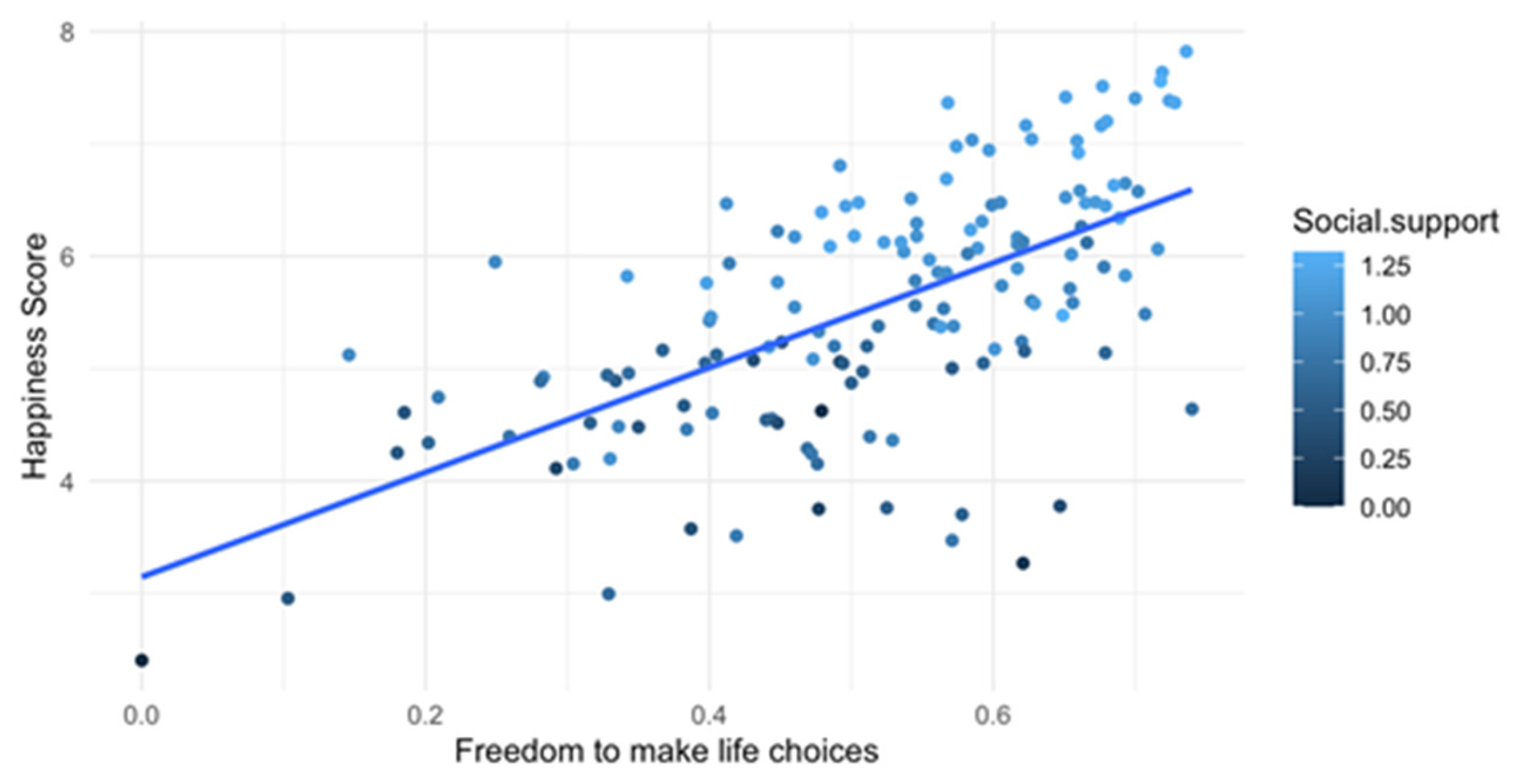
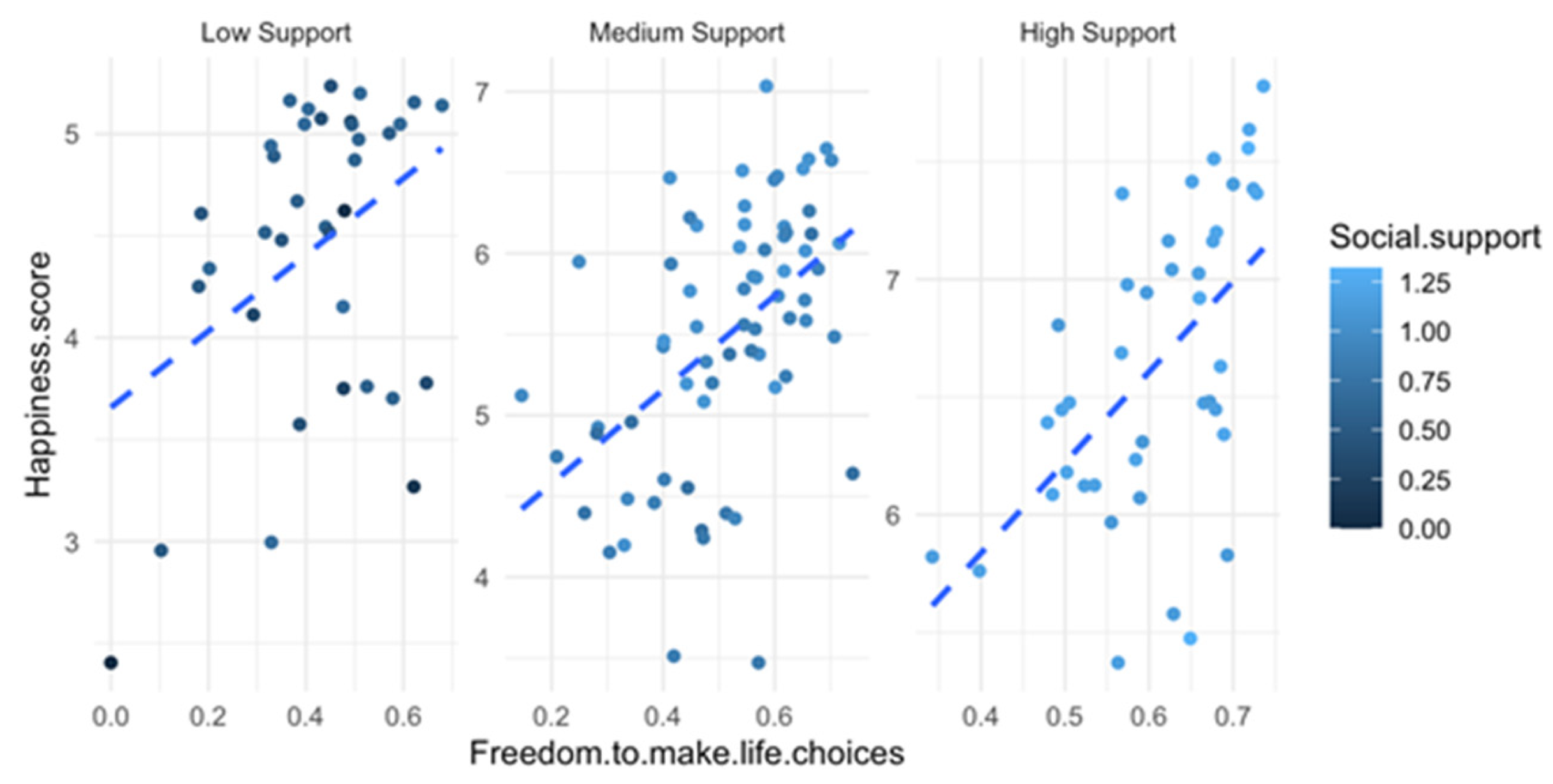
The scatter plot (Figure 6) shows how the ability to make life choices influences happiness for different levels of social support. The positive correlation between freedom to make life choices and happiness score indicates that greater freedom in decision-making is associated with higher happiness levels. On the other hand, low social support is distributed across all levels of happiness, indicating that low social support does not always mean low happiness, but it may limit it. Finally, lighter points (high social support) are mostly above the regression line, suggesting that greater social support amplifies the positive effect of freedom on happiness. We must point out that some low-happiness points exist even when freedom is high, indicating that other factors might also play a role. High variance at high freedom levels indicates that freedom alone does not fully determine happiness—social support and other influences matter.

The effect of freedom of choice on happiness seems to be amplified by social support. When social support is low, the freedom of choice has a smaller impact on happiness. In societies with high social support, freedom from discrimination has a strong effect on happiness (Figure 7).

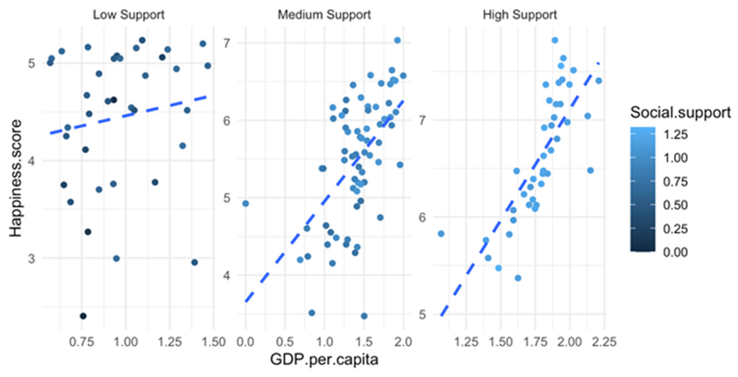
Similarly, it was examined how the GDP influences happiness for different levels of social support (Figure 8). GDP is a strong predictor of happiness—the greater the GDP, the greater the happiness score. On the other hand, social support plays a crucial role: darker points (low social support) are more scattered below the regression line, suggesting that even with higher GDP, low social support may limit happiness levels; lighter points (high social support) are clustered in the upper-right region, reinforcing that strong social support enhances happiness, particularly in wealthier nations. Finally, other factors likely contribute to happiness, as seen in scattered lower points.

The effect of GDP on happiness appears to be moderated by social support. In societies with high social support, GDP has a stronger impact on happiness. In societies with low social support, happiness seems less dependent on wealth (Figure 9). Slightly different results were obtained by Araki et al. [7] who found that the correlation between economic growth, quantified by changes in GDP per capita, and overall life satisfaction appears to decrease in societies that show increased economic standards. This development leads to an offsetting effect of GDP in the most prosperous countries.

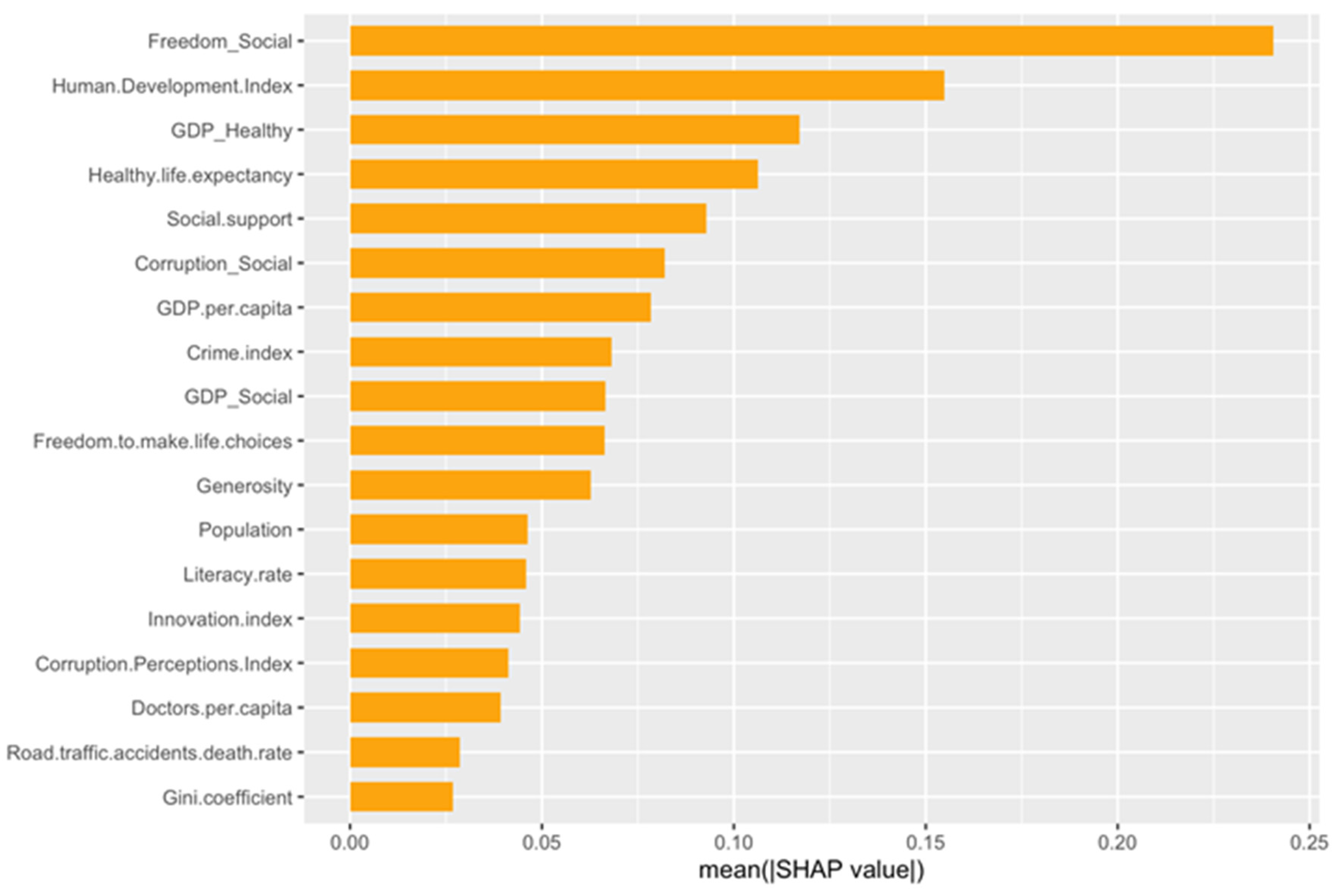
The most important variables using the XGBoost model (including interactions) for happiness is the interaction between freedom to make choices and social support (Figure 10), which is consistent with the result from the random forest model. The interaction between social support and GDP has a great impact too, as in the random forest. The variables deleted from the random forest model appear to have little impact.

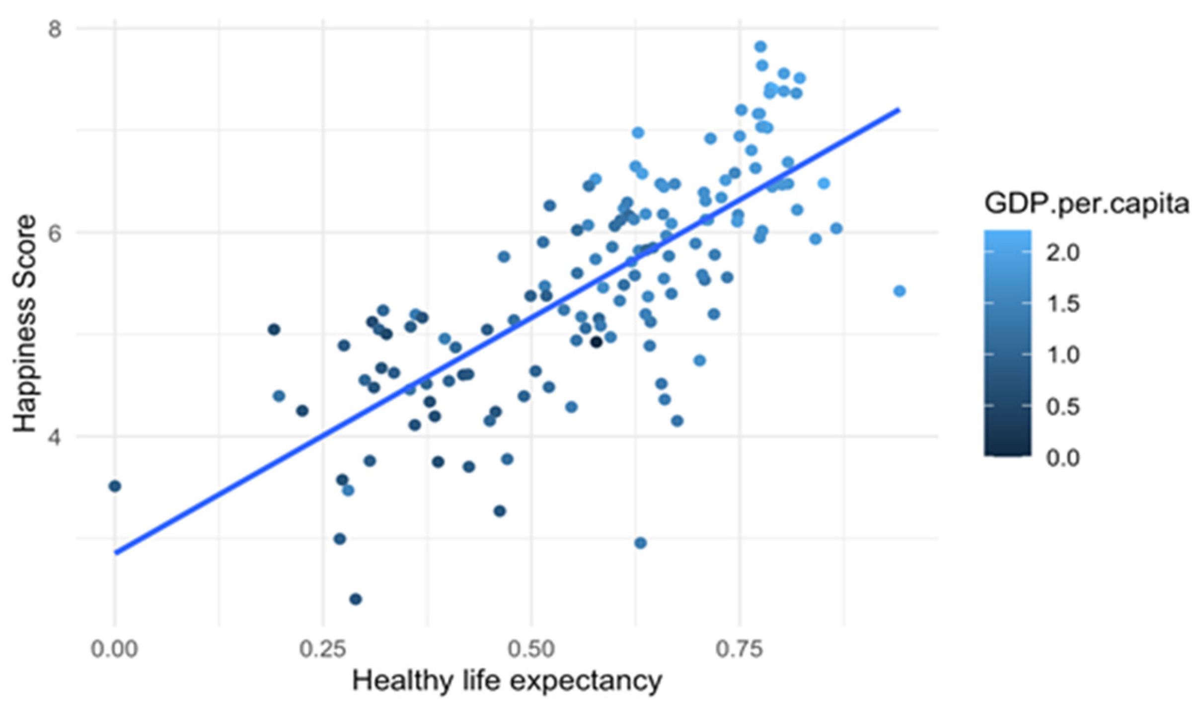
The scatter plot presented in Figure 11 shows how healthy life expectancy influences happiness for different values of GDP. There is a strong positive correlation between healthy life expectancy and happiness score, as shown by the upward trend and fitted regression line. Countries where people live longer in good health tend to report higher levels of happiness. The colour gradient indicates that higher GDP per capita (lighter blue) is generally associated with both higher happiness scores and longer healthy life expectancy, reinforcing the idea that economic wealth supports both well-being and longevity. Some dispersion exists around the trend line, suggesting that while health and happiness are closely linked, other socioeconomic or cultural factors also influence well-being.

The effect of healthy life expectancy on happiness appears to be moderated by GDP per capita. Low and Medium GDP groups show a positive correlation, meaning that longer healthy life expectancy is associated with greater happiness. High GDP countries exhibit a slightly negative or weak correlation, suggesting that once economic prosperity reaches a certain level, other factors may influence happiness more than life expectancy (Figure 12). Therefore, we can conclude that in lower-income countries, improving health conditions significantly enhances happiness. However, in wealthier nations, happiness may depend more on social, psychological, or lifestyle factors beyond just longevity.

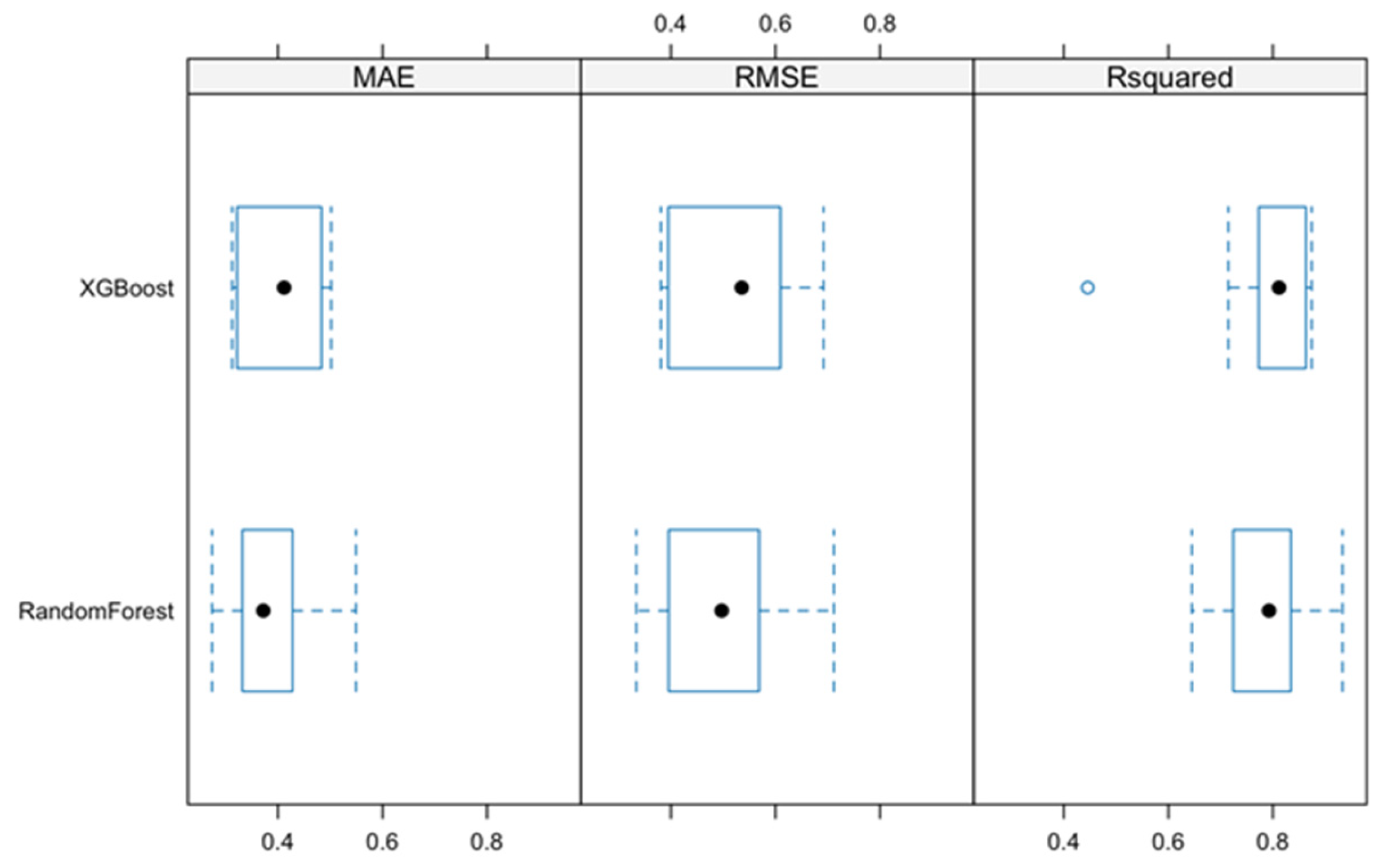
The comparison between machine learning decision tree-based models highlights that XGBoost achieved higher accuracy with a lower RMSE and a higher R², making it the preferred model. Both models identified the interaction between freedom to make life choices and social support as the most influential variable, suggesting a strong link between perceived freedom and happiness. Additionally, the Human Development Index, the interaction between GDP and Healthy life expectancy, social support, and the interaction between corruption perceptions index and social support were consistently ranked as important across both models, confirming their relevance. Nevertheless, there are aspects in which the results of the models differ: the XGBoost model ranked Human Development Index and Healthy life expectancy higher in importance compared to the Random Forest model, suggesting that these factors contribute significantly to the predictions made by XGBoost; the Random Forest model placed greater emphasis on Freedom to make life choices and in the interaction between GDP and Social Support, which were ranked lower in the XGBoost model; Crime Index appeared as a more influential factor in XGBoost, whereas it had a relatively lower ranking in the Random Forest model. Both models highlight the importance of freedom, economic factors, and social support in predicting happiness. However, variations in the ranking of some variables highlight differences in how each model processes feature interactions. After cross validation with 10 folds, the XGBoost and the Random Forest are quite close, with a slight advantage for the XGBoost, which has fewer errors (Figure 13). Since RMSE penalises larger errors, this metric reinforces that XGBoost may be able to predict extreme values more accurately than Random Forest. Both models have high R² values, indicating good fit in given years. The XGBoost seems to present a slightly higher and more stable R² (lower dispersion), suggesting that it better captures the given variations. There is an outlier in XGboost, which may indicate that it has more difficulties in some cross-validation iterations. It is difficult to conclusively decide, based on the literature, which of the decision tree-based models better describes the relationship between happiness score and predictors. According to Akanbi [19], XGBoost was found to be better (R² = 0.85), while according to Jannani [20], RF is the best (R² = 0.94). In the present study, the better fit was shown by the XGBoost model with R² = 0.99.

Araki [7] concluded that gross domestic product and corruption are significant determinants of happiness. However, in this study, freedom to make life choices emerged as the most influential factor. Li and An [3] also emphasised the negative impact of corruption on happiness. This study differs from previous ones not only in the broader set of variables included in the models but also in the novel insights it provides, such as the importance of the literacy rate, a factor rarely highlighted in earlier research.

Moreover, the interaction between the perception of corruption index and social support was identified as significant by two structurally different models: linear regression with interaction terms and random forest. This suggests that the effect of social support on happiness is moderated by the level of corruption (note that higher values of the Corruption Perceptions Index indicate lower levels of perceived corruption). Li et al. [3] reported a direct quantitative relationship, stating that a 10% increase in the CPI leads to a 0.23 decrease in well-being. In contrast, our study provides a more nuanced interpretation, showing that the impact of individual factors such as GDP depends on the country’s level of development, as proxied by social support levels. Future research could improve causal interpretation by incorporating methods such as instrumental variable analysis or longitudinal panel data models to address potential endogeneity between variables like GDP and happiness.

These findings contribute to the ongoing theoretical discourse on the drivers of subjective well-being, reinforcing the idea that happiness is multidimensional and cannot be explained by GDP alone. From a policy perspective, the results underscore the importance of enhancing freedom of choice, reducing corruption, and improving access to basic services as effective strategies for boosting happiness—particularly in low- and middle-income countries. These insights reinforce the notion that sustainability is not only about environmental or economic stability, but also about fostering societies where citizens can lead fulfilling and autonomous lives. Integrating happiness and well-being metrics into policy frameworks can enhance the long-term sustainability of social development strategies. These findings support a multidimensional understanding of happiness and suggest that policies aiming to improve well-being should not focus exclusively on economic growth. Strengthening social safety nets, ensuring personal freedoms, and reducing perceived corruption can substantially increase population-level happiness, especially in less developed regions.

5. Limitations

Although the Happiness Score provides a useful global benchmark, it relies on a single-item self-assessment. As such, it may not fully capture the multidimensional nature of happiness, which is better assessed through composite, multi-item scales. This limitation should be addressed in future studies.

The second important limitation of this study concerns the potential cultural variability in the perception and expression of happiness. Although we employed a standardised Happiness Score to enable international comparisons, it is important to acknowledge that the meaning and experience of happiness can differ significantly across cultural contexts. The uniform application of such a metric may not fully reflect these cultural nuances, potentially influencing the comparability of results. Therefore, future research should incorporate culturally sensitive approaches, including qualitative methods and panel studies, to more comprehensively explore subjective well-being.

6. Conclusions

The analysis of data from 145 countries highlights several key insights into the drivers of happiness. This study successfully identified the necessary and sufficient conditions for high happiness levels by combining statistical approaches (GLM, PCA) with configurational analysis (fsQCA), fulfilling the objective outlined at the outset. First and foremost, freedom to make life choices emerged as one of the strongest predictors of higher Happiness Scores across all models, indicating that individuals’ sense of autonomy plays a central role in overall well-being. Moreover, social support and corruption perceptions consistently interact with other factors, most notably GDP per capita and healthy life expectancy, illustrating that those greater economic resources and longer, healthier lives yield the highest returns when accompanied by transparent institutions and communal bonds. Interestingly, although the crime rate did not universally appear as a dominant factor, the literacy rate did exhibit a direct influence on happiness. This underlines the importance of education, not only in raising living standards but also in supporting more autonomous, fulfilling lives. The decision tree approaches (Random Forest and XGBoost) reinforced the centrality of the interaction between freedom and social support in predicting happiness. XGBoost demonstrated slightly stronger predictive power, emphasising the importance of modelling non-linear, complex relationships in well-being research. A fuzzy set-based qualitative comparative analysis (fsQCA) showed that no single factor or combination of factors is sufficient to guarantee high levels of happiness. A set of factors necessary for a high sense of happiness was identified, but this combination (or any other considered) is not a sufficient set—guaranteeing happiness.

Collectively, these findings underscore that happiness is multidimensional. Policies aimed at improving quality of life should therefore address diverse elements in tandem—bolstering education, reducing corruption, expanding social networks, providing economic stability, and safeguarding the individual freedom to choose. By recognising the interplay of these factors, governments, institutions, and communities can better foster environments where genuine well-being can thrive.

In addition to the global analysis, our results reveal important regional distinctions. For instance, in African countries, variables such as freedom of choice and corruption perceptions played a more prominent role than economic indicators. In contrast, in European countries, income and life expectancy showed stronger associations with happiness levels. These contrasts suggest that public policies aiming to improve happiness should be context-specific, taking into account the socio-economic and cultural realities of each region. The limitation of this study is the inability to control for individual-level sociodemographic factors such as age, gender, or education level, due to the aggregated nature of the dataset. Future studies using microdata would allow for more granular analysis.

Cultural issues analysis was conducted in this study. We consider that it should be explored in a future study that focuses specifically on these characteristics. The longitudinal study of happiness is considered a highly relevant area of research. In this context, the estimation and exploration of panel data is a suggestion for future studies.