Intelligent Control of the Main Steam Flow Rate for the Municipal Solid Waste Incineration Process

Abstract

The stable control of the main steam flow rate (MSFR) can effectively improve the waste combustion efficiency and energy utilization, reduce environmental pollution, and is crucial for promoting the sustainable development of municipal solid waste incineration (MSWI). Developed countries benefit from stable municipal solid waste (MSW) composition, enabling advanced automated combustion control. However, in developing countries, fluctuating waste composition and calorific value cause frequent disturbances, limiting the use of foreign control methods. Therefore, MSFR control technologies suited to developing countries are crucial. This study proposes a two-layer intelligent control method, consisting of an optimization setting layer and a loop control layer. The optimization layer uses a steam flow prediction model (OPTICS and RBF) and an improved antlion optimizer (IALO) for manipulated variable setpoints. The control layer applies reinforcement learning (actor–critic) to fine-tune PI controller parameters. Experimental results show that the proposed method adaptively adjusts manipulated variables, ensuring MSFR control within the target range and maintaining efficient, stable MSWI operation.

1. Introduction

Pollution control remains a critical issue for global sustainable development [1]. With the acceleration of urbanization, the annual generation of municipal solid waste (MSW) worldwide continues to grow steadily at a rate of 8–10% [2]. In developing countries where waste classification systems are not yet well-established, the problem of “waste surrounding cities” has become increasingly severe [3]. Therefore, effective measures must be taken to address the growing volume of waste in order to prevent further environmental deterioration. Compared to traditional waste management methods, municipal solid waste incineration (MSWI) offers significant advantages and can effectively reduce pollution. Traditional methods such as landfilling and open burning often lead to land and air pollution, whereas MSWI converts waste into energy through advanced combustion technologies. This not only alleviates environmental pressure but also recovers thermal energy, promoting sustainable urban development. However, during the incineration process, the stable control of the main steam flow rate (MSFR) is one of the key factors for the stable operation of the MSWI system. Stable control of MSFR can improve energy efficiency, reduce emissions, and promote resource recycling [4,5]. Therefore, stable control of the MSFR is crucial for both the MSWI operation and the sustainable development of cities.

In developed countries, waste separation systems are well implemented. This results in relatively uniform MSW composition and stable calorific values. Such conditions provide a solid foundation for applying automated combustion control strategies [6]. However, in developing countries, where waste classification is still under development, MSW composition and calorific value fluctuate widely. These fluctuations cause frequent disturbances in incineration, making it difficult to directly apply control strategies developed abroad [7]. Therefore, the effective MSFR control technologies tailored to developing countries’ complex conditions are essential for improving incineration stability and pollution control efficiency.

Thanks to rigorous classification and standardized pretreatment, developed countries have created stable incineration environments. Highly automated control systems further ensure these environments are well controlled. This provides ideal conditions for advanced mechanistic model-based control strategies [8,9]. For example, a pioneering two-stage closed-loop identification method was proposed [10], which introduces an input sensitivity function to reduce the impact of disturbances on modeling accuracy. This approach produced a multiple-input multiple-output (MIMO) model that maintained MSFR prediction errors below 4% at the HVC incineration plant in the Netherlands. Building on this, a nonlinear model predictive control (MPC) system based on a three-zone combustion model was developed [11]. By optimizing grate speed and secondary air distribution, the system decoupled MSFR and carbon monoxide emissions and reduced steam flow response delay to 80 s, greatly improving dynamic performance. Another study applied MPC to MSFR control by constructing a precise predictive model [12] that accounted for variations in waste composition and equipment status. This method significantly enhanced MSFR control stability and accuracy.

The above mechanistic modeling and advanced control methods, grounded in stable operation conditions, provide valuable theoretical and practical foundations for global MSWI control technologies. However, in developing countries, kitchen waste accounts for more than 50% of MSW, leading to high moisture content and low calorific value. These factors severely reduce combustion stability and cause MSFR to be highly sensitive to fuel disturbances [13]. There is a strong coupling among furnace temperature, flue gas oxygen concentration, and MSFR during incineration [14]. Empirical data show that every 5% increase in moisture content expands the MSFR fluctuation range by ±1.2% [15]. This makes it difficult to directly transfer control strategies from developed countries to practical applications in developing countries.

To address these challenges of varying operating conditions in developing countries, researchers have carried out systematic technological innovations based on data-driven approaches and intelligent algorithms. Traditional PI parameter tuning methods are unsuitable due to changes in process characteristics [16,17], an event-triggered RBF–PID controller is developed in [18]. It can adaptively adjust PID parameters based on dynamic furnace temperature changes. It reduces MSFR recovery time under load disturbances to 120 s while keeping fluctuations within ±2%. To better serve control objectives, a fuzzy-width forest regression soft sensing method is proposed in [19], maintaining MSFR prediction errors within ±3.5% even under calorific value fluctuations of ±15%. A Takagi–Sugeno (TS) fuzzy neural network is employed to achieve nonlinear decoupling among multiple variables in [20], keeping MSFR prediction errors below 5%, further improving control accuracy. Additionally, advances in swarm intelligence have opened new perspectives for MSFR control [21,22]. For instance, the beetle antennae search–support vector machine (BAS–SVM) algorithm, inspired by swarm behavior, achieves global optimization of control variables. It balances multiple objectives, including steam flow stability, energy efficiency, and pollutant emissions [23]. This method enhances system adaptability, robustness, and optimization, greatly improving steam flow control effectiveness.

Although the previous studies have significantly improved system control performance, several key technical challenges remain. For example, in multivariable decoupling, relative gain array (RGA)-based methods reduce coupling to some extent [24], but MSWI involves complex pyrolysis, gasification, and combustion reactions. The strong nonlinearity and uncertainty often cause model mismatch, limiting these methods’ broad application. More importantly, existing control strategies mainly focus on precise tracking of target variables but lack the ability to dynamically optimize control setpoints [25]. However, in dynamic operating conditions, the predefined setpoints often deviate from their optimal values. In such cases, experienced operators must manually adjust parameters such as airflow based on empirical judgment. Yet, when the composition of waste varies significantly or combustion conditions fluctuate rapidly, expert intervention may be delayed or inconsistent due to differences in individual expertise, experience, and skill levels. This subjectivity can hinder effective steam flow regulation and compromise overall system performance. Reference [26] addresses the issue of varying operating conditions by proposing a two-layer control architecture for operational management and hydroelectricity production maximization in inland waterways. It eliminates the subjective errors introduced by manual settings.

Developing countries face challenges due to immature waste sorting systems, large fluctuations in waste composition and calorific value, and frequent changes in combustion conditions. This makes it difficult to achieve automated combustion control like in developed nations. To address this, we propose a two-layer intelligent control system for the MSFR. The system proposed in the paper accounts for computational and infrastructure limitations while handling changing conditions. Regarding hardware limitations, we use a two-layer structure in the system design. The optimization setting and loop control layers operate on separate devices. This reduces reliance on a single device and ensures better task distribution. The system can adjust control parameters in real-time, based on current conditions. A PI controller tracks the new set points, ensuring stable and efficient operation. On the other hand, the antlion optimization (ALO) and reinforcement learning algorithms are innovative but have existing applications. Local technicians in developing countries can perform routine maintenance after proper training, reducing reliance on external experts and lowering costs. Furthermore, the system uses buffering and data interpolation. This ensures stable operation even when data acquisition devices are incomplete or delayed. Therefore, the main contributions of this study are as follows:

(1)

An RBF neural network prediction model was established at the optimization setting level to accurately predict the MSFR. By introducing the OPTICS algorithm, the centers and widths of the RBF hidden layer were objectively determined, and the gradient descent algorithm was used to adaptively adjust the neural network parameters. The model’s accuracy and good convergence were validated through experiments involving five different models (BP neural network, RBF neural network, RBF neural network with maximum matrix element algorithm, and RBF neural network with K-means clustering).

(2)

Additionally, optimization setting of the manipulated variables based on IALO is proposed. The manipulated variables’ setting values can be dynamically adjusted in response to changes in operating conditions.

(3)

In the control layer, reinforcement learning was introduced to the PI control system, which can quickly track the set values, especially when operating conditions change, with the PI parameters automatically tuned. Compared to the QDRNN-PID control system and the standard PID control system, the proposed intelligent optimization control method for MSFR demonstrated strong robustness and dynamic response capabilities.

The remainder of this article is organized as follows. Section 2 analyzes the MSWI process and control problems. Section 3 introduces the methodology of the MSFR control. Section 4 discusses experimental results. Finally, Section 5 concludes this article.

2. Control Problem Description in the MSWI Process

2.1. Description of MSWI Process Flow

A typical municipal solid waste incineration (MSWI) process flow is shown in Figure 1, which consists of six key systems working in synergy: the solid waste fermentation system, solid waste combustion system, waste heat recovery system, steam generation system, flue gas filtration system, and flue gas emission system. In the solid waste combustion system, pre-treated solid waste, after classification, is conveyed to the incinerator through a hopper. The solid waste undergoes complete combustion within the system, releasing substantial thermal energy, which is transferred as high-temperature flue gas to the waste heat recovery system. In this system, the high-temperature flue gas flows sequentially through the water-cooled wall, economizer, evaporator, and superheater of the waste heat boiler, enabling efficient heat exchange with water or steam. During this process, water is gradually heated into saturated steam. It is then further converted into high-temperature, high-pressure superheated steam. This steam is known as the main steam. This main steam not only heats the primary and secondary air for the combustion system but also serves as the key driving force for the turbine generator in the steam power generation system. Therefore, the stable control of the MSWI MSFR is crucial for the stable operation of both the solid waste incineration and steam generation systems [27,28,29,30].

The MSFR is closely linked to the heat exchange processes in the solid waste combustion and waste heat boiler systems. In the combustion system, high-precision temperature sensors monitor the furnace temperature in real time, pressure sensors detect furnace pressure, and airflow sensors measure the speeds of primary and secondary air. These data serve as critical inputs for precise combustion control. The flow control valves for both air streams are adjusted in real time based on sensor feedback, while the grate speed motor modulates grate speed as needed. Similarly, in the waste heat recovery system, temperature and pressure sensors monitor the steam’s state in real time. Typically, a throttling device measures the MSFR. However, due to fluctuations in solid waste composition, environmental temperature changes, and the dynamic behavior of steam temperature, pressure, and flow rate, accurately measuring the MSFR is often challenging.

2.2. Problem Analysis

To effectively control the MSF, it is first essential to analyze the influencing factors from a mechanistic perspective. This involves considering the interactions among multiple variables and their dynamic variations to identify truly feasible and critical control variables [31]. The MSFR mechanism model established in reference [32] is shown in Equation (1). The MSFR is closely related to factors such as primary and secondary air.

$$y={\displaystyle \frac{\left(Q_{in}-Q_{loss}\right)+\sqrt{{\left(Q_{in}-Q_{loss}\right)}^2-4\left(h_{sh}-h_{ws}\right)\cdot 5.82{\left(S_{rated}\right)}^{0.62}}}{2\left(h_{sh}-h_{ws}\right)}},$$

(1)

$$Q_{in}=Q_{ncv}+Q_{air,\mathsf{I}}+Q_{air,\mathsf{I}\mathsf{I}},$$

(2)

where $Q_{in}$ and $Q_{loss}$ are the input heat and heat loss, respectively; $h_{sh}$ and $h_{ws}$ are the enthalpies of superheated steam and feedwater; $S_{rated}$ is rated MSFR; $Q_{ncv}$ is the basic low-grade heat received; $Q_{air,\mathsf{I}}$ and $Q_{air,\mathsf{I}\mathsf{I}}$ are the heat contributions from primary and secondary air; and $Q_{loss}$ represents the total heat loss caused by physical heat loss from slag, incomplete combustion of solid materials, and flue gases in the incinerator.

Apart from airflow, the MSFR is also influenced by factors such as the boiler drum pressure, secondary air fan outlet pressure, economizer feedwater flow, and grate speed [11,33]. Firstly, the boiler drum pressure directly regulates the steam generation rate by altering the steam-water separation efficiency, steam storage conditions, and the phase change conditions of water, thus affecting the MSFR. Secondly, the secondary air fan outlet pressure determines the motive force for secondary air entering the furnace, which influences the oxygen supply during combustion and the airflow distribution. Thereby affecting the combustion intensity and stability, ultimately impacting the MSFR. The economizer feedwater flow, as the material basis for steam generation, not only determines the amount of water involved in steam production but also influences the system’s thermal balance, playing a crucial role. Additionally, the grate speed determines the residence time of the solid waste within the furnace, influencing the degree of combustion and the heat release process. Thus, the MSFR is primarily affected by the primary and secondary airflow rates, secondary air fan outlet pressure, boiler drum pressure, economizer feedwater flow, and grate speed.

Since abrupt changes in grate speed may cause shifts in the combustion zone and its distribution, affecting the stability of the combustion process, and given its slow response and complex impacts, it is typically not used as a direct control variable. However, changes in grate speed can comprehensively reflect information on the characteristics of solid waste, combustion conditions, and the system’s thermal balance, making it an important parameter for characterizing the operating conditions of municipal solid waste incineration (MSWI) [34]. Therefore, in this study, primary airflow rate, secondary airflow rate, secondary air fan outlet pressure, boiler drum pressure, and economizer feedwater flow are chosen as control variables.

The complex and variable composition of solid waste, coupled with drift in operating conditions, results in a highly coupled nonlinear relationship between the control variables and the MSFR, making it difficult to describe the relationship through mathematical models precisely. Hence, the relationship between the MSFR and its influencing factors is shown in Equation (3) and Figure 2, where $f(·)$ represents the complex nonlinear relationship describing the connection between the MSFR and six influencing factors. S₁, S₂, S₃, S₄, and S₅ are the control variables, and $\Omega$ represents the operating conditions as characterized by the grate speed.

$$y=f\left(S_1,S_2,S_3,S_4,S_5,\Omega \right).$$

(3)

3. Methodology

The objective of the MSFR control is shown in Equations (4) and (5). It is to maintain the steam flow within the target range required by the process and to bring it as close as possible to the target MSFR value.

$$\min \left\{\left|y-y^{\ast }\right|\right\},$$

(4)

$$-\tau \le y-y^{\ast }\le \tau ,\tau >0,$$

(5)

where $y$ represents the measured MSFR, and $y^{\ast }$ represents the target MSFR. The absolute deviation between the target and the measured MSFR must satisfy the condition of not exceeding epsilon $\tau$.

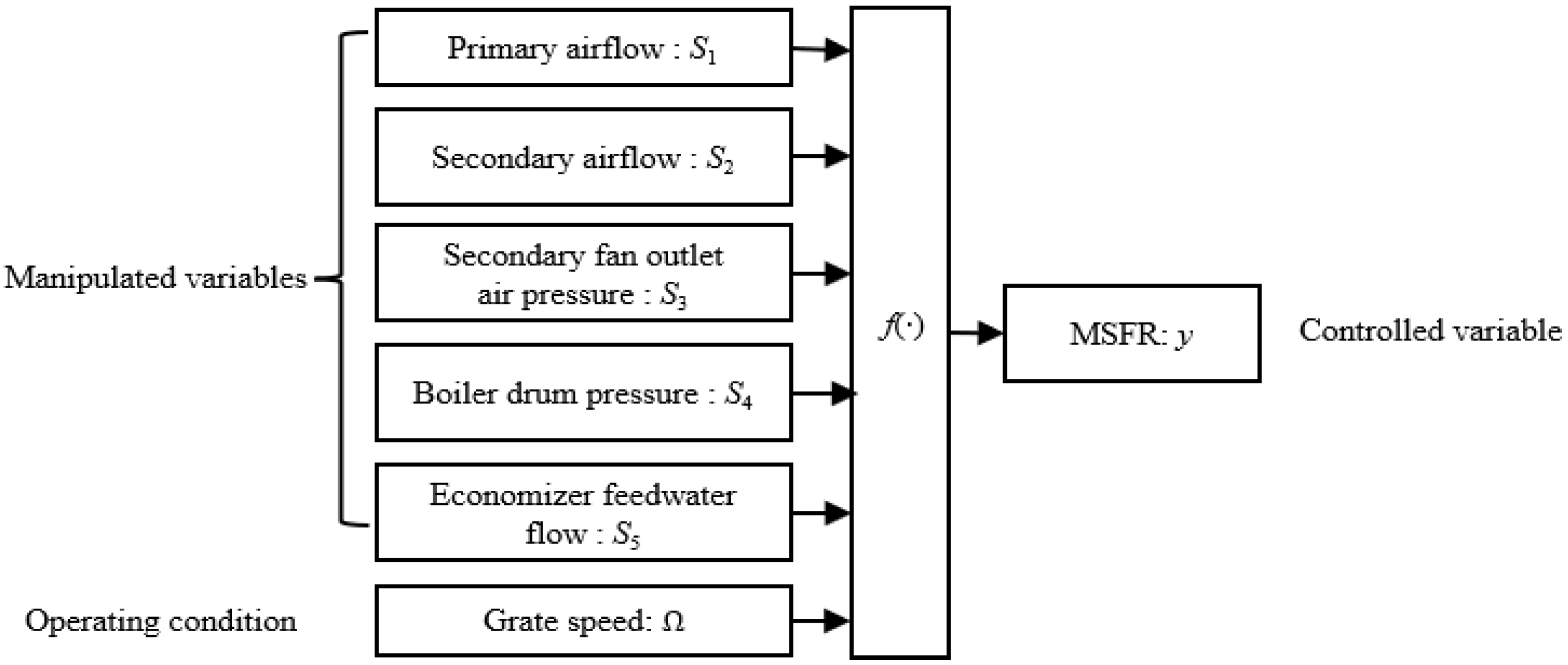
The achievement of this objective relies on the coordinated regulation of several key parameters, including primary airflow $S_1$, secondary airflow $S_2$, secondary air fan outlet pressure $S_3$, boiler drum pressure $S_4$, and economizer feedwater flow $S_5$. The grate speed serves as an indicator of changes in operating conditions. Since fluctuations in solid waste composition and changes in environmental temperature can lead to dynamic changes in operating conditions, the control system must not only focus on the loop’s tracking performance of setpoints but also investigate how to optimize the setpoints of key manipulated variables in real-time according to the changing operating conditions. To tackle this, this article proposes a two-layer intelligent control method that includes an optimization setting layer and a loop control layer, aiming to maintain the MSFR within the target range while ensuring the combustion process operates in an optimized state. Essentially, this problem is a multivariable nonlinear optimization issue in a dynamic environment [35].

Inspired by the application of the antlion optimizer to solve the nonlinear optimization problem of multivariable manipulated variables in voltage source converters [36]. The antlion optimizer is applied in the setpoint optimization layer [37]. On the other hand, the RBF technique is used to solve the nonlinear modeling problem of the alkali borosilicate glass transition temperature [38]. Given the nonlinear fitting capability of RBF neural networks to asymptotically approximate real values, which has been widely applied in modeling complex nonlinear industrial processes [39], the RBF technique is used to model the nonlinear relationship between the MSFR and its influencing factors. In the loop control system, the incorporation of reinforcement learning techniques is considered. Reinforcement learning, as a function approximation-based approach, has achieved significant success in solving complex tasks with high-dimensional state spaces and nonlinear control problems, such as robot control [40]. We explored integrating reinforcement learning into the design of the loop control system. A variable PI controller is developed to enhance the system’s adaptability, aiming at the complex operating conditions [41,42].

3.1. Intelligent Control Strategy

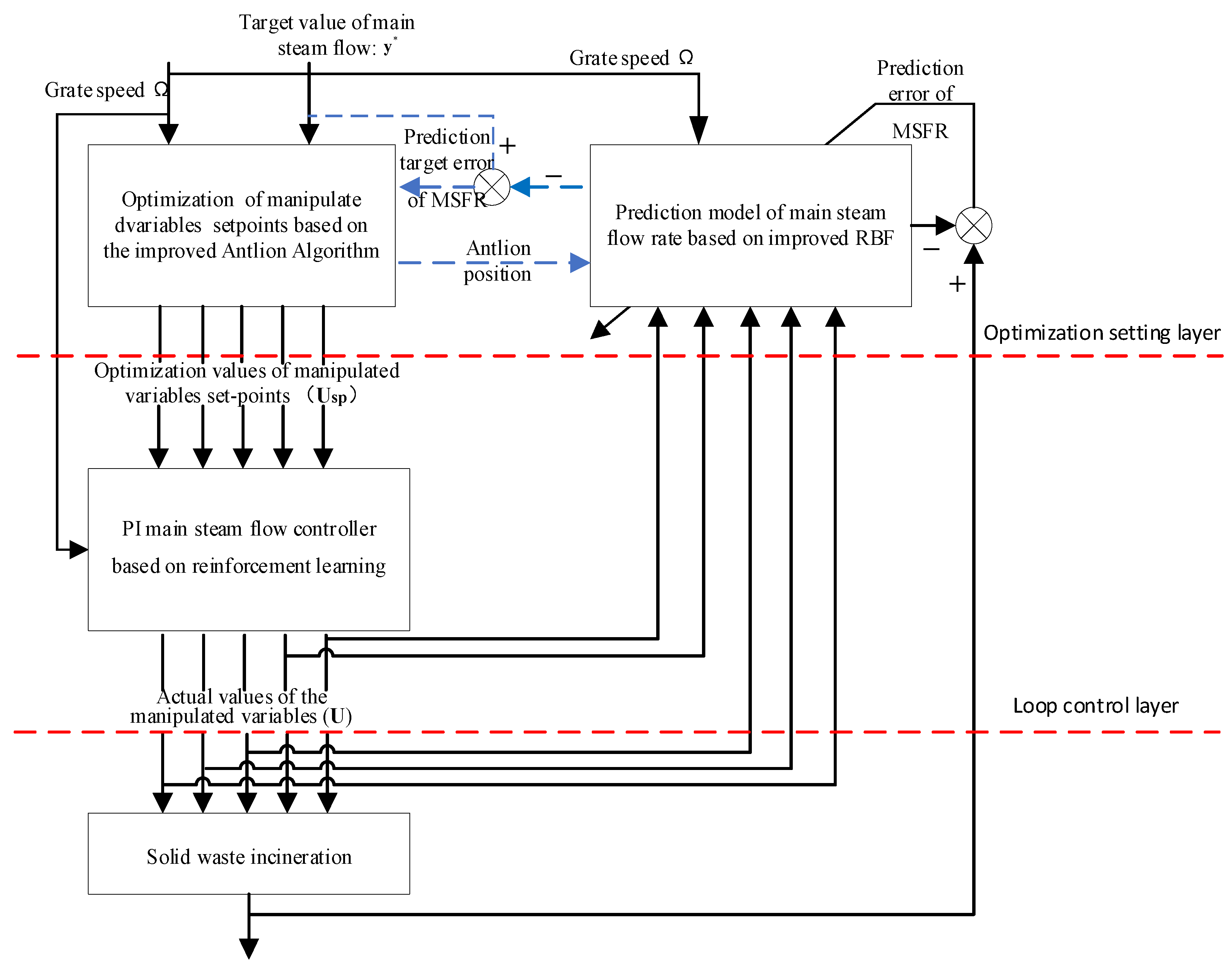
In consideration of the multivariable, nonlinear, and dynamic characteristics of the MSFR control problem within the MSWI system, this article presents a two-layer intelligent control method, as depicted in Figure 3. The method comprises a manipulated variables optimization setpoint layer and a loop control layer. There are three key modules: the MSFR prediction module based on the improved RBF, the manipulated variables optimization setpoints module based on the improved antlion algorithm, and the PI loop control system module based on reinforcement learning. Within the MSFR prediction module relying on the improved RBF, the inputs incorporate key manipulated variables ($S_1–S_5$) and the grate speed, which characterizes the operating conditions. This module utilizes RBF techniques for modeling and employs gradient descent algorithms to conduct self-learning of the model’s key parameters, ultimately yielding the predicted MSFR for the MSWI. The manipulated variables optimization setpoint module, relying on the improved antlion algorithm, uses the target MSFR as an input and optimizes the key manipulated variables ($S_1–S_5$) via the improved antlion algorithm. The PI MSFR control system module, which relies on reinforcement learning, constitutes a PI control system. It utilizes the grate speed, which represents operating conditions, and the optimized key manipulated variables ($S_1–S_5$) as inputs. This module applies reinforcement learning techniques. The module is designed to enable the adaptive adjustment of PI parameters by changing operating conditions, thus achieving more precise and efficient MSFR control.

3.2. Intelligent Control Algorithm

3.2.1. MSFR Prediction Module Based on the Improved RBF

(1)

Model Structure

The MSFR prediction module utilizes a three-layer RBF neural network composed of an input layer, a hidden layer, and an output layer. The input layer comprises six nodes, which correspond to the key manipulated variables ($S_1–S_5$) and the grate speed ($\Omega$), the latter of which characterizes the operating conditions. The output layer is composed of a single neuron that represents the predicted value of the MSFR ($\widehat{y}$). The quantity of nodes in the hidden layer is determined by means of the OPTICS clustering algorithm. The nodes within the hidden layer employ a Gaussian radial basis function,

$${\phi }_g(x)=\exp (-{\displaystyle \frac{{‖x-c_g‖}^2}{2{\sigma }_g^2}}),$$

(6)

$$\widehat{y}={\displaystyle \sum _{g=1}^m{\phi }_g(x){\omega }_g},$$

(7)

where $x=\left(u,\Omega \right)$, $x\in R^6$, represents the inputs; m is the number of hidden layer nodes; and ${\mathbf{c}}_g$ is the center of the g-th radial basis function. The values of m and ${\mathbf{c}}_g$ are determined using the OPTICS clustering algorithm; ${\sigma }_g$ is the width parameter of the neuron; and ${\omega }_g$ is the connection weight between the g-th hidden layer node and the output layer node, which are determined using the gradient descent algorithm. The network output is the predicted MSFR value $\widehat{y}$.

(2)

Determination of RBF hidden layer node number m and parameter $c_g$ based on the OPTICS clustering algorithm

The OPTICS clustering algorithm was chosen over DBSCAN and K-means++ because it can better handle data with varying densities, noise, and uncertain cluster numbers, and it does not require the number of clusters to be set in advance, offering greater flexibility and accuracy.

The Euclidean distance formula is used to calculate the distance metric between sample data points.

$${\mathit{D}}_{ij}=dist(x_i,x_j)=\sqrt{{\displaystyle \sum _{s=1}^6{(x_{is}-x_{js})}^2}},$$

(8)

where $x_i,x_j\in R^6$ represent the inputs vectors of two sample data in a six-dimensional space; and $x_{is},x_{js}$ are the values of the s-th dimension.

The core distance is defined as follows:

$$dis{t}_{core}(x_i)=\min \left\{(\epsilon ||\psi (x_i,\epsilon )|\ge w)\right\},$$

(9)

$$\psi (x_j,\epsilon )=\left\{x_j\right|dist(x_i,x_j)\le \epsilon \},$$

(10)

where $\epsilon$ represents the neighborhood range radius of the MSFR; and $w$ is the number of MSFR samples which are within the range $\epsilon$. The reachable distance is defined as follows:

$$dis{t}_{reach}(x_o,x_j)=\max (dis{t}_{core}(x_j),dist(x_o,x_j)).$$

(11)

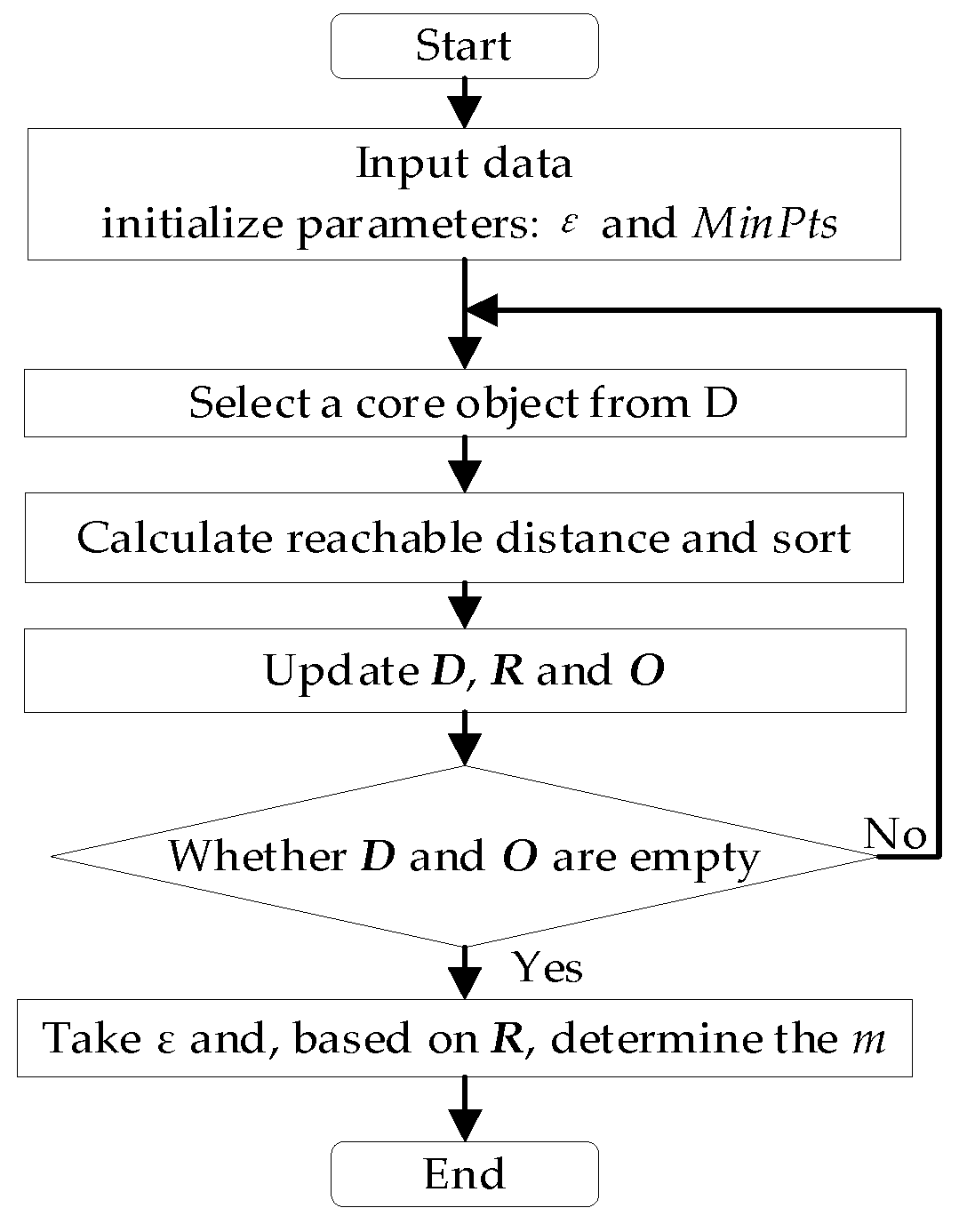
The specific clustering process is shown in Figure 4 and is described as follows:

• Step 1: Input the sample data of manipulated variables and operating conditions, initialize the reachable distances, and create an ordered queue O and a result queue R.
• Step 2: Use Equation (8) to calculate the dataset D, and compute all the core distances using Equation (9).
• Step 3: Select an object from D as the core object P, place it into R, and remove it from D. Use Equation (11) to calculate the reachable distance of other data points to the core object P, sort them by reachable distance, and add them to O.
• Step 4: Select the data point with the smallest reachable distance from O as the new core object P, place it into R, and remove it from both O and D. Calculate the reachable distance of the remaining data points to the new core object, and update O.
• Step 5: Check if O and D are empty. If not, repeat Step 4.
• Step 6: Take $\epsilon$ and, based on R, determine the number of clusters m.

After determining the number of clusters m, and the center points of the RBF, hidden layer neurons are determined using Equation (12).

$${\mathbf{c}}_g={\displaystyle \frac{1}{N}}{\displaystyle \sum _{j=1}^N{x}_j},$$

(12)

where N represents the total number of data points in the g-th cluster of MSFR, and $x_j$ denotes the sample belonging to this cluster.

(3)

Correction of RBF neural network parameters ${\sigma }_g$ and ${\omega }_g$ based on the gradient descent algorithm.

The gradient descent algorithm is used to update the width parameter ${\sigma }_g$ of the neurons and the output layer weights ${\omega }_g$. The loss function is defined as follows:

$$E_{loss}={\displaystyle \frac{1}{2}}{\displaystyle \sum _{i=1}^N{‖y_i-{\widehat{y}}_i‖}^2},$$

(13)

where $y_i$ and ${\widehat{y}}_i$ represent the measured and predicted values of the MSFR for the i-th sample, respectively. The updated formulas for the neuron width parameter ${\sigma }_g$ and the output layer weights ${\omega }_g$ are as follows:

$${\sigma }_{g+1}={\sigma }_g-\eta {\displaystyle \frac{\partial E_{loss}}{\partial {\sigma }_g}},$$

(14)

$${\omega }_{g+1}={\omega }_g-\eta {\displaystyle \frac{\partial E_{loss}}{\partial {\omega }_g}},$$

(15)

$$-\eta {\displaystyle \frac{\partial E_{loss}}{\partial {\omega }_g}}=\eta {\displaystyle \sum _{i=1}^n({\widehat{y}}_i-y_i){\phi }_g(‖{\mathbf{x}}_i-{\mathbf{c}}_g‖)},$$

(16)

$$-\eta {\displaystyle \frac{\partial E_{loss}}{\partial {\sigma }_g}}=\eta {\displaystyle \frac{{\omega }_g}{{\sigma }_g^3}}{\displaystyle \sum _{i=1}^n({\widehat{y}}_i-y_i){\phi }_g(‖{\mathbf{x}}_i-{\mathbf{c}}_g‖){‖{\mathbf{x}}_i-{\mathbf{c}}_g‖}^2},$$

(17)

where $\eta$ denotes the learning rate. The update formulas are derived through the calculation of the partial derivatives of the loss function with respect to the neuron width parameter ${\sigma }_g$ and the output layer weights ${\omega }_g$. This enables the correction of the error function along the direction of the negative gradient, facilitating the iterative optimization of the parameters.

3.2.2. Optimization of Manipulated Variables Setpoint Based on the IALO

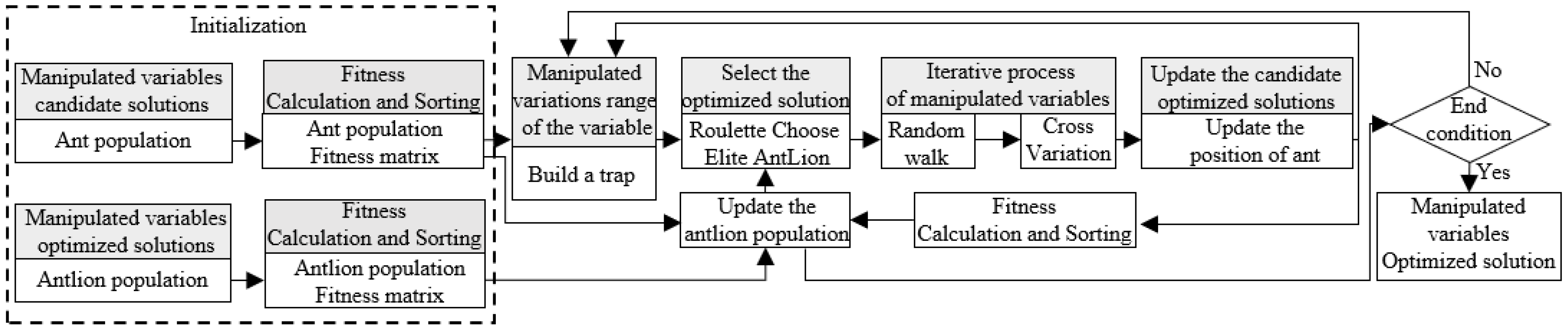
The optimization of the manipulated variables setpoint based on the IALO for the MSFR is designed to optimize the manipulated variables based on the input target value of the MSFR. The optimization is performed using the IALO algorithm, with the strategy diagram shown in Figure 5. The module randomly generates candidate solutions for the manipulated variables and their optimized counterparts. The MSFR prediction model is then used to predict the MSFR for each solution, from which the fitness is calculated. The antlion algorithm attracts ants toward the optimal manipulated variables solutions by constructing traps. The ants adjust their positions through random walks, while the elite antlions guide the search process. The solutions for both ants and antlions are merged and sorted, and continuously updated until the termination conditions are met. The optimized manipulated variables are ultimately output to ensure the MSFR reaches the target value. In the event of a change in the operating conditions, such as furnace grate speed, the manipulated variables will be re-optimized.

The objective function $f_{obj}$ and fitness function $f_{fit}$ for the optimization of the MSFR are presented by the equations as follows:

$$f_{fit}={\displaystyle \frac{1}{1+f_{obj}}},$$

(18)

$$f_{obj}={\displaystyle \frac{{\displaystyle \sum _{i=1}^{100}\sqrt{{(y_i-{\widehat{y}}_i)}^2}}}{100}},$$

(19)

where $y_i$ and ${\widehat{y}}_i$ represent, respectively, the measured and predicted values of the MSFR for the i-th sample. The value of ${\widehat{y}}_i$ is determined via the MSFR prediction model.

Table 1. The relationship between the improved antlion algorithm and the optimization of MSFR.

Parameters in the Ant-Lion Algorithm	Manipulated Variables Optimization Problem
Ant	A candidate solution for manipulated variables
Ant population	The set of candidate solutions for manipulated variables
Antlion	One round of iterative manipulated variables optimization solution
Antlion population	Manipulated variables optimization solution set
The movement of ants The hunting behavior of antlions Elite antlion	Search for the optimization solution process of manipulated variables Update the optimization solution of the manipulated variables The optimized solution of manipulated variables

shows the relationship between the improved antlion optimizer and the MSFR parameter optimization problem. The ants represent candidate solutions for the manipulated variables, the antlion represents the optimized solution for the manipulated variables, and the elite antlion represents the global optimized solution for the manipulated variables.

The antlion optimization algorithm draws inspiration from the predatory behavior of antlions in the natural realm and their interactions with ants. The algorithm involves a series of steps to find the optimal solution, including the random walk of ants, the construction of traps by the antlions, ants being trapped, the antlions capturing their prey, and the reconstruction of traps. The process is described as follows:

(1)

The random walk of ants and the normalization process.

$$H\left(l\right)=[0,cumsum\left(2r\left(l_1-1\right)\right),\dots ,cumsum\left(2r\left(l_l-1\right)\right].$$

(20)

$$r(l)=\left\{\begin{array}{lll}1& if& rand>0.5\\ 0& if& rand\le 0.5\end{array}\right..$$

(21)

In the given equation, the cumulative $cumsum$ is calculated, and rand represents a random number uniformly distributed within the interval [0, 1].

$$H_s^l=E\left[{\displaystyle \frac{(H_s^l-a_s)\times (d_{\mathrm{s}}^l-c_s^l)}{(b_s-a_s)}}+c_s^l\right],$$

(22)

where $a_s$ and $b_s$ represent, respectively, the minimum and maximum values of the random walk for the s-th dimension of the manipulated variables; $c_s^l$ and $d_s^l$ denote the minimum and maximum values of the manipulated variables in the l-th iteration for the s-th dimension; and E is the error between the predicted and target values of the MSFR. The five-dimensional manipulated variables ($S_1–S_5$) are primary airflow, secondary airflow, secondary fan outlet air pressure, boiler steam drum pressure, and economizer feedwater flow.

Two improvements are proposed based on the antlion optimization algorithm to tackle the problems of premature convergence and getting trapped in local optima during the optimization of the MSFR manipulated variables. Firstly, an adaptive step-size factor is introduced during the random movement of the ants, which dynamically adjusts the search step size to enhance search efficiency and avoid premature convergence. Secondly, during the update of the ants’ positions, crossover and mutation operations from genetic algorithms are integrated to increase the diversity of the population. It can prevent the algorithm from converging to local optima and enhance its global search capability.

Improvement 1: The position update strategy is given by the following equation:

$$H_s^l=E\left[{\displaystyle \frac{(H_s^l-a_s)\times (d_s^l-c_s^l)}{(b_s-a_s)}}+c_s^l\right]\times \xi ,$$

(23)

$$\xi ={\displaystyle \frac{L-l}{L}},$$

(24)

where L denotes the maximum number of iterations, and l represents the current iteration number.

$$H^{l’}=\left\{\begin{array}{ll}\hfill H_{1:s}^l\cup H_{s+1:5}^{l-1}& ifrand<0.8\hfill \\ \hfill X^{l}if& rand\ge 0.8\hfill \end{array}\right..$$

(25)

$$H_s^{l″}=l{b}_s+(u{b}_s-l{b}_s)\cdot rand().$$

(26)

In the given equation, $u{b}_s$ and $l{b}_s$ represent the lower and upper bounds of the search space for the s-th dimension of the MSFR.

(2)

The antlion constructs traps that affect the random movement of ants within the search domain. This effect can be represented as follows:

$$\begin{array}{l}{c}_s^l=Antlio{n}_s^l+c^l\\ d_s^l=Antlio{n}_s^l+d^l\end{array},$$

(27)

where $c_s^l$ and $d_s^l$ represent, respectively, the minimum and maximum values of the manipulated variables in the s-th dimension during the l-th iteration; and $Antlio{n}_s^l$ represents the position of the antlion in the s-th dimension during the l-th iteration.

(3)

To simulate the process of ants approaching the antlions, the boundaries of the random movement should be gradually narrowed.

$$\begin{array}{l}{c}^l={\displaystyle \frac{c^l}{I}}\\ d^l={\displaystyle \frac{d^l}{I}}\end{array}.$$

(28)

In the given equation, $I=1+{10}^v{\displaystyle \frac{l}{L}}$, l represents the current iteration index, and L represents the maximum number of iterations, while V must adhere to the following condition:

$$\left\{\begin{array}{ll}v=2& l>0.1L\\ v=3& l>0.5L\\ v=4& l>0.75L\\ v=5& l>0.9L\\ v=6& l>0.95L\end{array}\right..$$

(29)

(4)

During the process of the antlion capturing prey, if the value of the objective function of an ant is superior to that of the selected antlion, the position of the antlion will be replaced by the most recent position of the captured ant, thereby enhancing the probability of capturing ants. The equation is presented as follows:

$$Antlio{n}_j^l=An{t}_j^l\begin{array}{cc}if& f(An{t}_j^l)\end{array}<f(Antlio{n}_j^l).$$

(30)

During the iteration process, the antlion with the highest fitness value in each generation is selected as the elite antlion. Additionally, another antlion is selected via the roulette wheel selection method. The random movements of all other ants are attracted to these two antlions. The equation is presented as follows:

$${\mathrm{Ant}}_i^l={\displaystyle \frac{H_A^l+H_E^l}{2}},$$

(31)

where $H_A^l$ and $H_E^l$ denote the positions of the ant after conducting a random movement, when the ant has to choose between the normal and elite antlion via the roulette wheel selection method during the l-th iteration.

3.2.3. PI Control System for MSFR Based on Reinforcement Learning

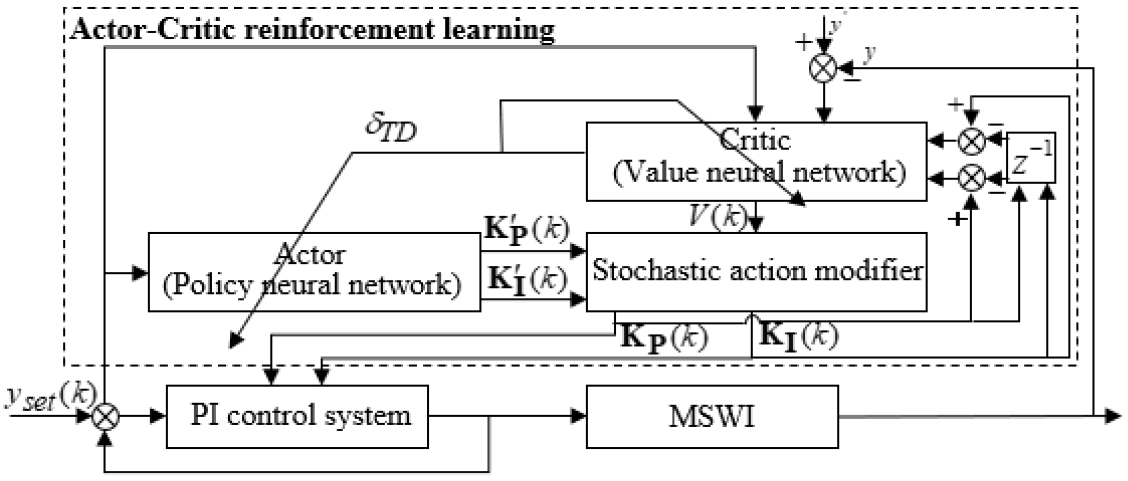
Traditional PI control systems perform suboptimally when confronted with strong nonlinearities and time-varying systems. In such cases, operators need sufficient experience to adjust the parameters manually. However, manual adjustments are time-consuming and often fail to achieve the desired results, especially in complex environments. To address this issue, this study adopts a reinforcement learning framework based on the actor–critic architecture and proposes a PI tuning method, as illustrated in Figure 6. The control system consists of three components: the actor (policy neural network), the critic (value neural network), and the Stochastic Action Modifier. Firstly, the actor (policy neural network) generates reference PI manipulated variables based on the setpoints of the manipulated variables and the grate speed provided by the optimization layer. Next, the critic (value neural network) computes the value function estimate based on the setpoints of the manipulated variables and the grate speed provided by the optimization layer. Finally, the Stochastic Action Modifier combines the reference PI values generated by the actor with the value function estimate produced by the critic to obtain the actual PI parameters for optimized system control. When the grate speed operating condition changes, the optimization layer adjusts the corresponding setpoints of the manipulated variables, and the reinforcement learning system updates the PI parameters according to variations in the grate speed and manipulated variable setpoints.

An incremental PI controller is designed as defined in Equation (32),

$$\begin{array}{ll}\mathbf{u}(k)& =\mathbf{u}(k-1)+\mathsf{\Delta }\mathbf{u}(k)\\ & =\mathbf{u}(k-1)+{\mathbf{K}}_{\mathbf{I}}(k)e(k)+{\mathbf{K}}_{\mathbf{p}}(k)\mathsf{\Delta }e(k)\end{array},$$

(32)

where $\mathsf{\Delta }e\left(k\right)=e\left(k\right)-e\left(k-1\right)$ and $e(k)=y_{set}(k)-y_r(k)$, where $y_{set}(k)$ is the setpoint of the manipulated variables, and is the actual value of the manipulated variables.

The RBF network is used to approximate both the policy function of the Actor and the value function of the Critic [43]. The policy and value neural networks share the input and hidden layers of the RBF network, which not only reduces memory requirements but also enhances learning efficiency. The AC learning structure based on RBF is illustrated in Figure 7.

(1)

Determination of PI values based on the RBF neural network

The three inputs of the RBF are $e(k)$, $\mathsf{\Delta }e(k)$ and $\Omega$, as shown in Equation (33).

$$\mathit{X}(k)=[e(k),\mathsf{\Delta }e(k),\Omega {]}^T.$$

(33)

The radial basis function of the hidden layer adopts the Gaussian kernel function as follows:

$${\varphi }_h(k)=\exp \left(-{\displaystyle \frac{{‖\mathit{X}(k)-{\mathit{c}}_h(k)‖}^2}{2{\sigma }_h^2(k)}}\right)$$

(34)

The output layer has 3 nodes, and the outputs are ${\mathbf{K}}_{\mathbf{P}}^{\prime }\left(k\right)$, ${\mathbf{K}}_{\mathbf{I}}^{\prime }(k)$, and the value function of the value neural network. The mathematical expression is as follows:

$${\mathbf{K}}_{\mathbf{P},\mathbf{I}}^{\prime }(k)={\displaystyle \sum _{h=1}^m{\omega }_h^{P,I}(k){\varphi }_h(k)},$$

(35)

$$V(k)={\displaystyle \sum _{h=1}^m{v}_h(k){\varphi }_h(k)},$$

(36)

where $v_h\left(t\right)$ represents the weight between the h-th hidden unit and the critic output layer, and ${\omega }_h^{P,I}$ represents the weight between the h-th hidden unit and the output layer of the actor.

To resolve the exploration–exploitation dilemma, the outputs from the Actor are not directly passed to the PI controller. Instead, a Gaussian noise term $n_k(0,{\varsigma }_V(k))$ is added to the recommended PI parameters ${\mathbf{K}}_{\mathbf{P},\mathbf{I}}^{\prime }(k)$ coming from the Actor. Thus, the actual PI parameters are modified as shown in Equation (37). The magnitude of the Gaussian noise depends on $V(k)$. When $V(k)$ is large, the noise term is small, and vice versa.

$${\mathbf{K}}_{\mathbf{P},\mathbf{I}}(k)={\mathbf{K}}_{\mathbf{P},\mathbf{I}}^{\prime }(k)+n_k(0,{\varsigma }_V(k)),$$

(37)

where ${\varsigma }_V(k)={\displaystyle \frac{1}{1+\exp \left(2V(k)\right)}}$.

(2)

Parameter update method for ${\omega }_h^{P,I}$, $v_h$, $c_h$, and ${\sigma }_h$ based on the gradient descent algorithm

The calculation of the error is as follows, using the temporal difference algorithm:

$${\delta }_{TD}(k)=R(k)+\gamma V(k)-V(k-1),$$

(38)

where $V\left(k\right)$ represents the value function, and $R\left(k\right)$ is the reward at k-th time; $\gamma$ denotes the discount factor. The reward R(k) is defined as follows:

$$R_{s_i}(k)=0.5{\left[{\mathbf{y}}^{\ast }(k)-y(k)\right]}^2-0.1\left(\left|\mathsf{\Delta }{K}_P^{s_i}\right|+\left|\mathsf{\Delta }{K}_I^{s_i}\right|\right)-0.6\cdot \left|e_{s_i}\right|,$$

(39)

where $\mathsf{\Delta }{K}_P^{s_i}$ and $\mathsf{\Delta }{K}_I^{s_i}$ are the change proportional and integral gain of each manipulated variable at the current moment k; $e_{s_i}$ is the error value of each manipulated variable; and ${\mathbf{y}}^{\ast }\left(k\right)$ and $y\left(k\right)$ are, respectively, the target value and measured value of the MSFR. The weights are updated using Equations (40) and (41),

$${\omega }_h^{P,I}(k+1)={\omega }_h^{P,I}(k)+{\eta }^{\prime }{\delta }_{\mathrm{TD}}(k){\displaystyle \frac{{\mathbf{K}}_{\mathbf{P},\mathbf{I}}(k)-{\mathbf{K}}_{\mathbf{P},\mathbf{I}}^{\prime }(k)}{{\sigma }_V(k)}}{\varphi }_h(k),$$

(40)

$$v_h(k+1)=v_h(k)-{\eta }^{″}{\delta }_{TD}(k){\varphi }_h(k),$$

(41)

where ${\eta }^{\prime }$ and ${\eta }^{″}$ are the learning rates of the policy neural network and the value neural network, respectively. The center $c_h$ and center width ${\sigma }_h$ of the neurons are updated using Equations (42) and (43),

$${\mathit{c}}_h(k+1)={\mathit{c}}_h(k)+{\eta }_c{\delta }_{TD}{v}_h(k){\varphi }_h(k){\displaystyle \frac{\mathit{X}(k)-{\mathit{c}}_h(k)}{{\sigma }_h^2(k)}},$$

(42)

$${\sigma }_h(k+1)={\sigma }_h(k)+{\eta }_{\sigma }{\delta }_{TD}{v}_h(k){\varphi }_h(k){\displaystyle \frac{{‖\mathit{X}(k)-{\mathit{c}}_h(k)‖}^2}{{\sigma }_h^3(k)}}.$$

(43)

3.3. Realization Steps of the Intelligent Control Method for MSFR

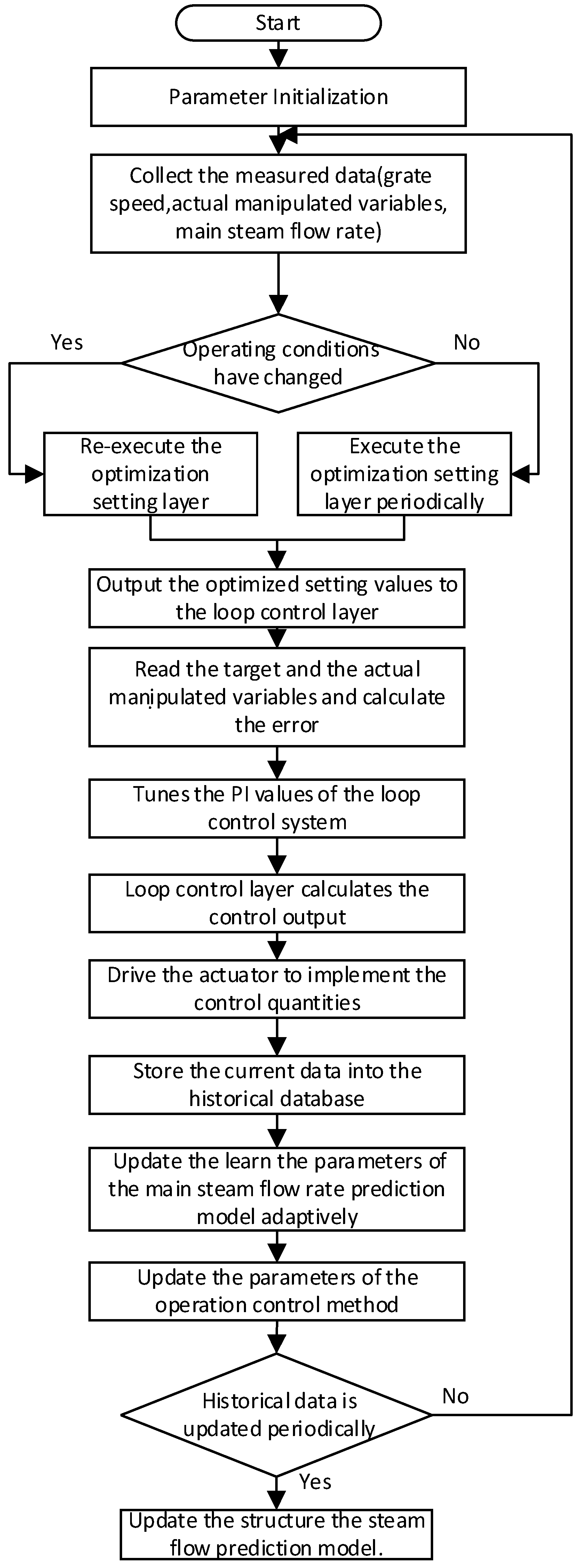
As shown in Figure 8, the steps for implementing the two-layer intelligent control method for the MSFR are as follows:

Step 1: Parameter Initialization: The ant population, antlion population, maximum number of iterations, and search range are initialized, and an initial solution is randomly generated within the search range.

Step 2: Collect the measured data, including the grate speed, the actual control values, parameters, and the measured MSFR.

Step 3: Identify whether the working operating conditions have changed. If the grate speed changes, re-execute the optimization setting layer at once. Otherwise, execute the optimization setting layer periodically.

Step 4: Output the optimized setting values of the manipulated variables and send them to the loop control layer to execute.

Step 5: Compute the error between the target and the actual manipulated variables.

Step 6: The loop control layer tunes the PI values of the loop control system according to Equations (35)–(37) and implements the optimized setting values of the manipulated variables based on Equation (32).

Step 7: Drive the actuator to implement the control quantities.

Step 8: Store the current data into the historical database, and update the learn parameters of the MSFR prediction model adaptively.

Step 9: Update the parameters of the intelligent control method.

Step 10: Is the historical data updated periodically? If yes, update the structure of the steam flow prediction model. If no, back to step 2.

Figure 8. The steps for implementing the two-layer intelligent control method.

Figure 8. The steps for implementing the two-layer intelligent control method.

4. Experiments and Analysis

In this section, we designed three experiments to validate the efficacy of the intelligent control approach for the MSFR presented in this article. All the experiments were conducted using on-site data collected from the DCS system of a forward-moving grate furnace in a waste incineration plant.

4.1. Verification of the MSFR Prediction Model Based on RBF

In this study, a total of 5000 sets of experimental data were used. The range of sample variations in the manipulated variables (primary and secondary airflow, secondary fan outlet air pressure, boiler drum pressure, and economizer feedwater flow) is as follows: $S_1\in \left[55,75\right]$, $S_2\in \left[0,11.4\right]$, $S_3\in \left[0,0,5\right]$, $S_4\in \left[4.4,4.6\right]$ and $S_5\in \left[30.5,35.3\right]$, and grate speed variations range is $\Omega \in \left[25,60\right]$. We took 3500 sets (70%) of the data as the training set for the MSFR prediction model, and 750 sets (15%) were used as the validation set. Another 750 sets (15%) were taken as the test set for the MSFR prediction model.

The OPTICS clustering algorithm uses six input variables of the MSWI system (primary airflow, secondary airflow, economizer feedwater flow, boiler drum pressure, secondary fan outlet air pressure, and grate speed under operating conditions) for clustering. The optimal combination of minimum sample size and neighborhood radius is determined through orthogonal experiments, with each parameter set at 5 levels. The minimum sample size is set at five levels: 4, 8, 12, 16, and 20. The initial neighborhood radius is set to infinity, and based on the reachable distance results obtained from the experiments, the neighborhood radius is divided into five levels: 0.11, 0.19, 0.27, 0.35, and 0.43.

Table 2. The number of clusters under each parameter combination.

Experiment Number	$\mathit{M}\mathit{i}\mathit{n}\mathit{P}\mathit{t}\mathit{s}$	$\mathit{\epsilon }$	Number of Clusters
1	4	0.11	13
2	4	0.19	22
3	4	0.27	17
⋮	⋮	⋮	⋮
24	20	0.35	32
25	20	0.43	27

shows the number of clusters for each parameter combination.

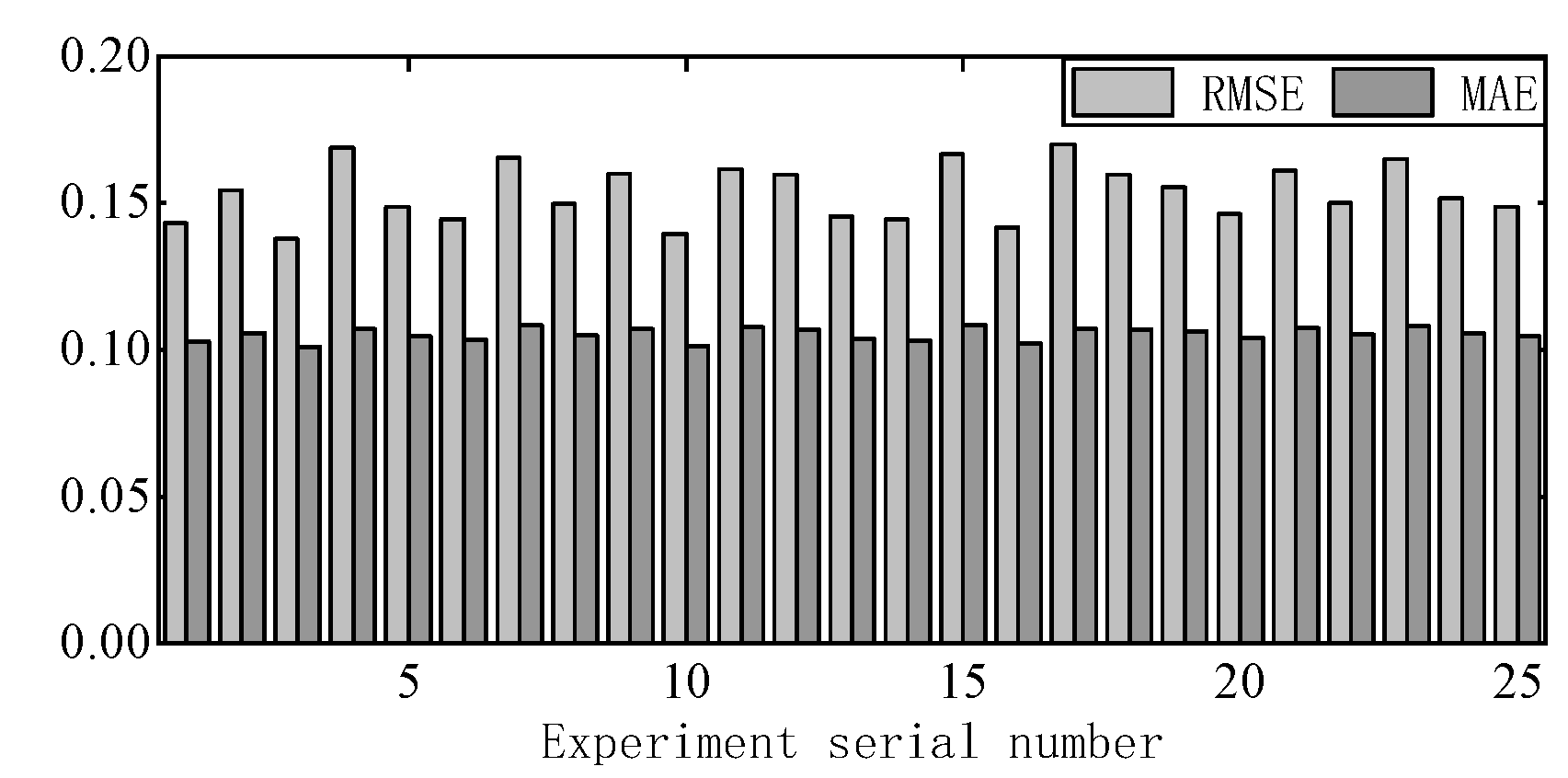
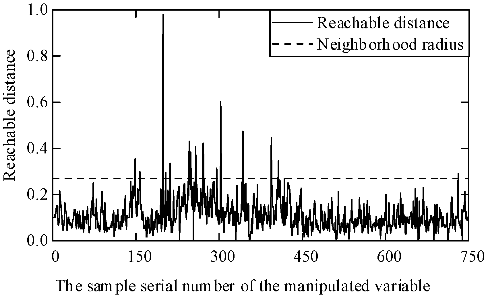
The neuron centers for each group of experiments are calculated using Equation (12). The model is trained using the training set data, with RMSE and MAE as performance evaluation metrics to determine the optimal parameter combination. Figure 9 shows the RMSE and MAE for each experimental combination. As can be seen from the figure, the model performs best when $MinPts=4,\epsilon =0.27$. Under this condition, Figure 10 shows the reachable distance sorting chart, while the corresponding neuron centers are listed in

Table 3. The MSFR RBF neural network $c_g$.

	Primary Airflow ${\mathit{S}}_1$	Secondary Airflow ${\mathbf{S}}_2$	Secondary Air Outlet Air Pressure ${\mathbf{S}}_3$	Boiler Drum Pressure ${\mathbf{S}}_4$	Economizer Feedwater Flow ${\mathbf{S}}_5$	Grate Speed $\mathsf{\Omega }$
1	55.528	1.234	0.135	4.548	33.108	40
2	58.334	1.317	0.132	4.554	33.488	40
3	63.737	0.750	0.061	4.561	33.667	40
⋮	⋮	⋮	⋮	⋮	⋮	⋮
16	61.723	9.957	0.404	4.593	33.197	60
17	70.873	10.220	0.401	4.574	33.636	60

.

To verify the effectiveness of the forecasting model, it is compared with the widely used BP neural network, RBF neural network, maximum matrix element (MME) RBF neural network, and K-means clustering-based RBF neural network models. The root mean square error is selected as the evaluation metric for the models. The training RMSE of each model is shown in Figure 11 and

Table 4. Comparison of five network forecasting models.

Model	RMSE (t/h)	MAE (t/h)	Model Structure
BP Neural Network	0.7903	0.6319	6-17-1
RBF Neural Network	0.5208	0.4015	6-17-1
MME-RBF Neural Network	0.4143	0.3287	6-34-1
K-means-RBF Neural Network	0.2656	0.2231	6-21-1
OPTICS-RBF Neural Network	0.1380	0.1009	6-17-1

. As can be seen, the proposed OPTICS-RBF neural network outperforms the other four neural networks in terms of faster convergence and higher accuracy.

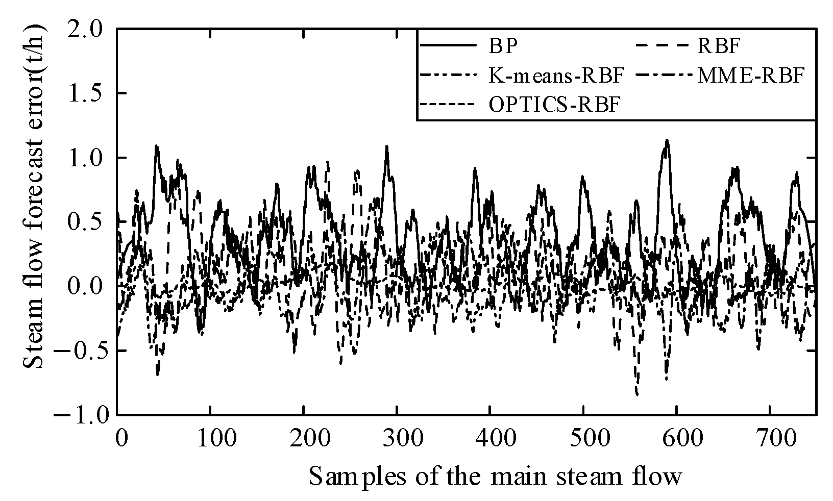
Experiments were conducted on the test set. Figure 12 and

Table 5. Comparison of the prediction error for the MSFR.

	Error Range (t/h)	RMSE (t/h)	MAE (t/h)	${\mathit{R}}^2$
BP Neural network	[−0.611, 1.930]	0.8916	0.6828	0.5112
RBF Neural network	[−1.350, 1.580]	0.5718	0.4379	0.6937
MME- RBF Neural Network	[−1.227, 1.267]	0.4767	0.3574	0.7663
K-means-RBF Neural network	[−0.823, 0.660]	0.2812	0.2363	0.8271
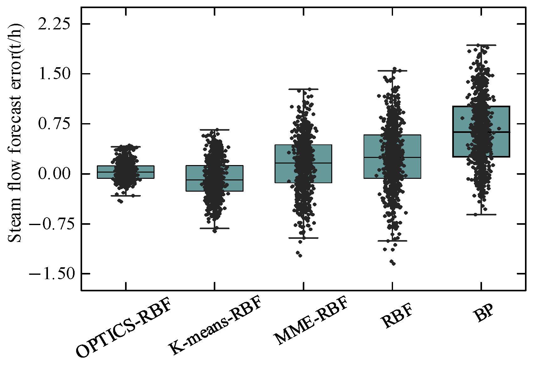
OPTICS-RBF Neural network	[−0.420, 0.429]	0.1692	0.1125	0.9218

present the errors between the predicted and actual values of the MSFR for five forecasting models on the test set. Figure 13 further visualizes the error distribution using a box plot. The results show that the OPTICS-RBF neural network has the smallest error range, which falls between [−0.420, 0.429].

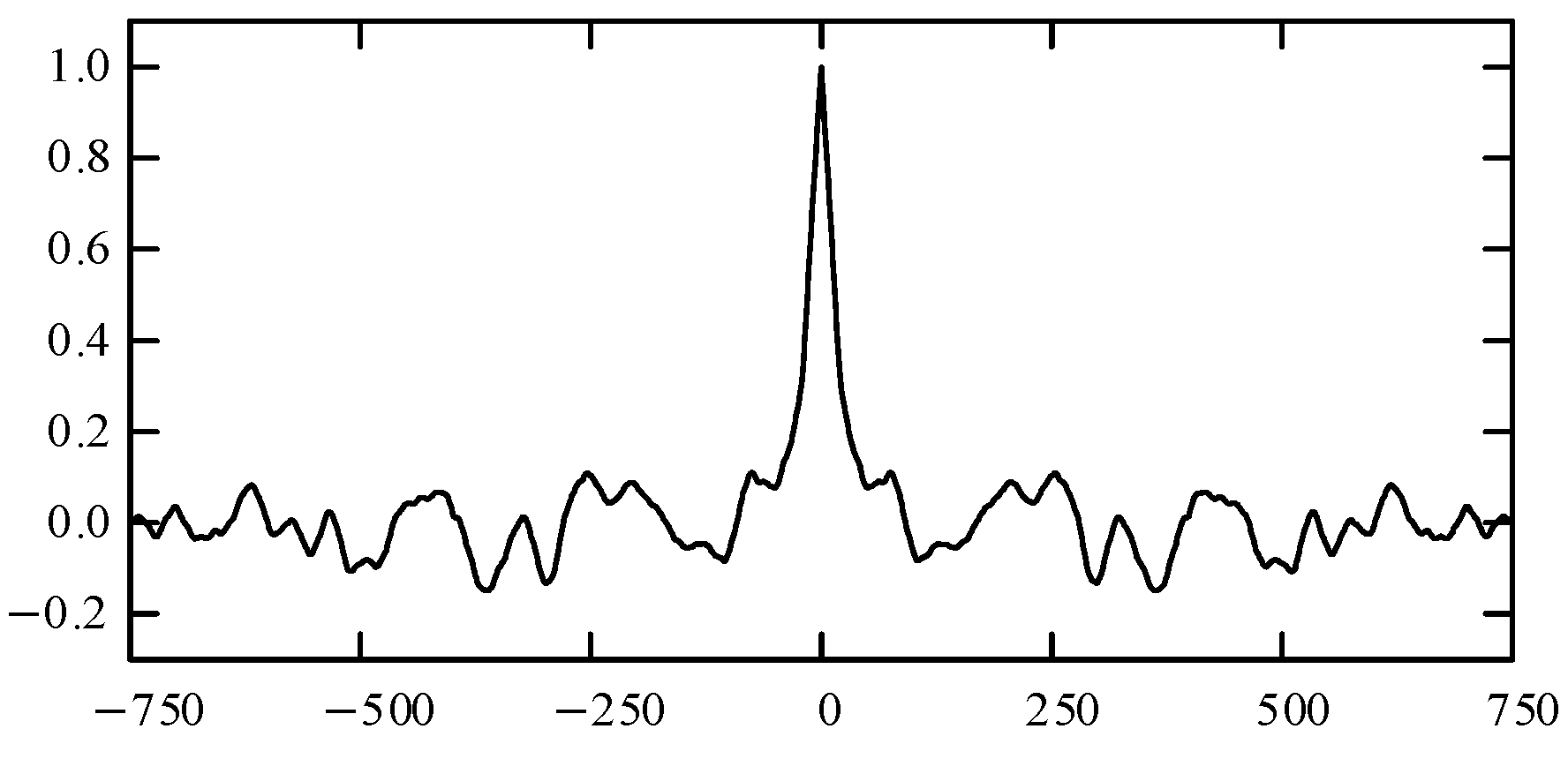
To further validate the effectiveness of the proposed MSFR forecasting model, Figure 14 shows the autocorrelation function of the normalized deviation between the predicted MSFR and the actual MSFR. From the figure, it can be observed that the autocorrelation coefficients of the deviation sequence mostly fall within the 95% confidence interval, indicating that the residual sequence can be considered as white noise.

4.2. Validation of the Intelligent Control Method

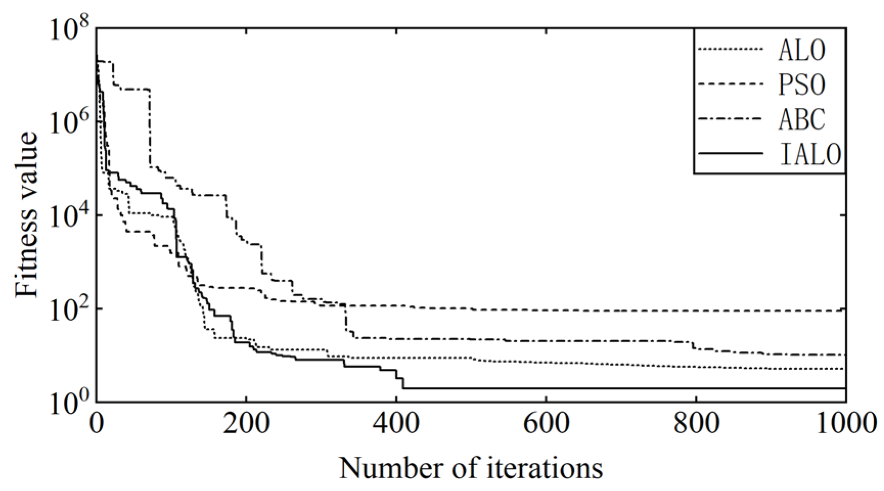
To verify the effectiveness of the IALO, it is compared with the widely used Particle Swarm Optimization (PSO) algorithm and Artificial Bee Colony (ABC) optimization algorithm. First, comparative tests are performed on the standard test functions shown in

Table 6. Unimodal reference function F5 and multi-modal reference function F12.

Function	Dimension	Range
$F_5(x)={\displaystyle {\sum }_{i=1}^{n=1}[100{({\mathbf{x}}_{i+1}-x_i^2)}^2}+{({\mathbf{x}}_i+1)}^2]$	50	[−30, 30]
$\begin{array}{c}{F}_{12}(x)={\displaystyle \frac{\pi }{n}}\left\{10\sin (\pi y_1)+{\displaystyle {\sum }_{i=1}^{n-1}{(y_i-1)}^2\left[1+{\sin }^2{(\pi y_{i+1})}^2\right]}+{(y_n-1)}^2\right\}\\ +{\displaystyle {\sum }_{i=1}^{n}u({\mathbf{x}}_{i,}10,100,4)}\end{array}$	50	[−50, 50]

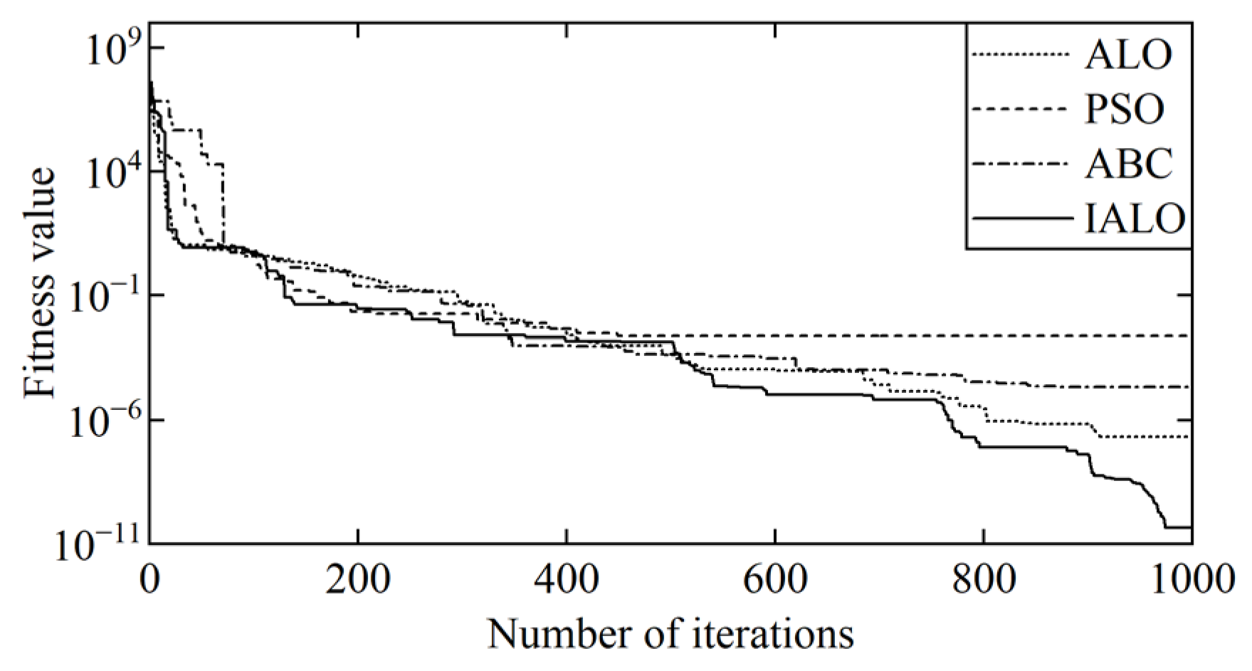
, where F5 is a unimodal benchmark function and F12 is a multimodal benchmark function. A total of 50 candidate solutions are set, and the number of iterations is 1000. For the unimodal benchmark function F5, the fitness change curve in Figure 15 shows that the ALO achieves a fitness value of 5.2827 at 957 iterations, PSO reaches a fitness value of 90.5459 at 988 iterations, ABC achieves a fitness value of 10.4729 at 922 iterations, and IAO achieves a fitness value of 1.9508 at 410 iterations. For the multimodal benchmark function F12, the fitness change curve in Figure 16 shows that ALO achieves a fitness value of 2.19 × 10⁻⁷ at 912 iterations, PSO reaches a fitness value of 0.0024 at 449 iterations, ABC achieves a fitness value of 2.12 × 10⁻⁵ at 872 iterations, and IALO achieves a fitness value of 4.69 × 10⁻¹¹ at 974 iterations. From the test results in

Table 7. Comparison of optimization results on the standard test functions.

	ALO	PSO	ABC	IALO
F5	5.2827	90.5459	10.4729	1.9508
F12	2.19 × 10−7	0.0024	2.12 × 10−5	4.69 × 10−11

, it can be concluded that the IALO proposed in this article exhibits better convergence and higher accuracy compared to ALO, PSO, and ABC.

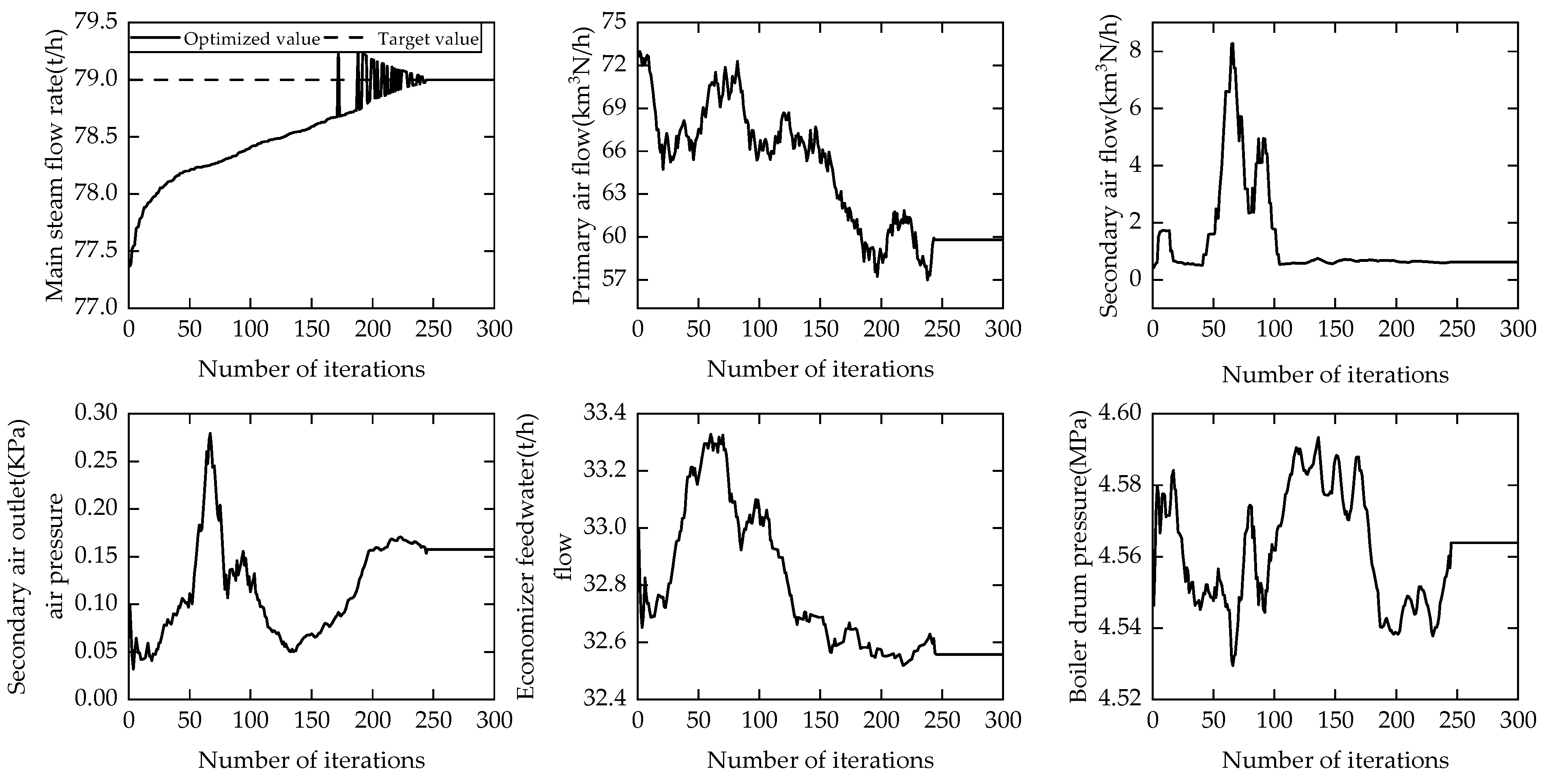
When validating the optimization setting of the manipulated variables based on IALO, the maximum number of iterations is set to 300, and the ant population is set to 40. Also, the antlion population is set to 40. The target MSFR value is 79. The search ranges of the primary airflow, secondary airflow, secondary fan outlet air pressure, boiler drum pressure, and economizer feedwater flow are $\left[55,75\right]$, $\left[0,11.4\right]$, $\left[0,0,5\right]$, $\left[4.4,4.6\right]$ and $\left[30.5,35.3\right]$. The optimization process is shown in Figure 17. After 243 iterations, the target values are found, where the corresponding parameters are primary airflow of 59.8, secondary airflow of 0.622, secondary fan outlet air pressure of 0.158, boiler steam drum pressure of 4.564, and economizer feedwater flow of 32.558.

4.3. Validation of the Effectiveness of the Intelligent Control Method Under Varying Operating Conditions

The purpose of this experiment is to verify whether the intelligent control method can effectively control the MSFR when operating conditions change.

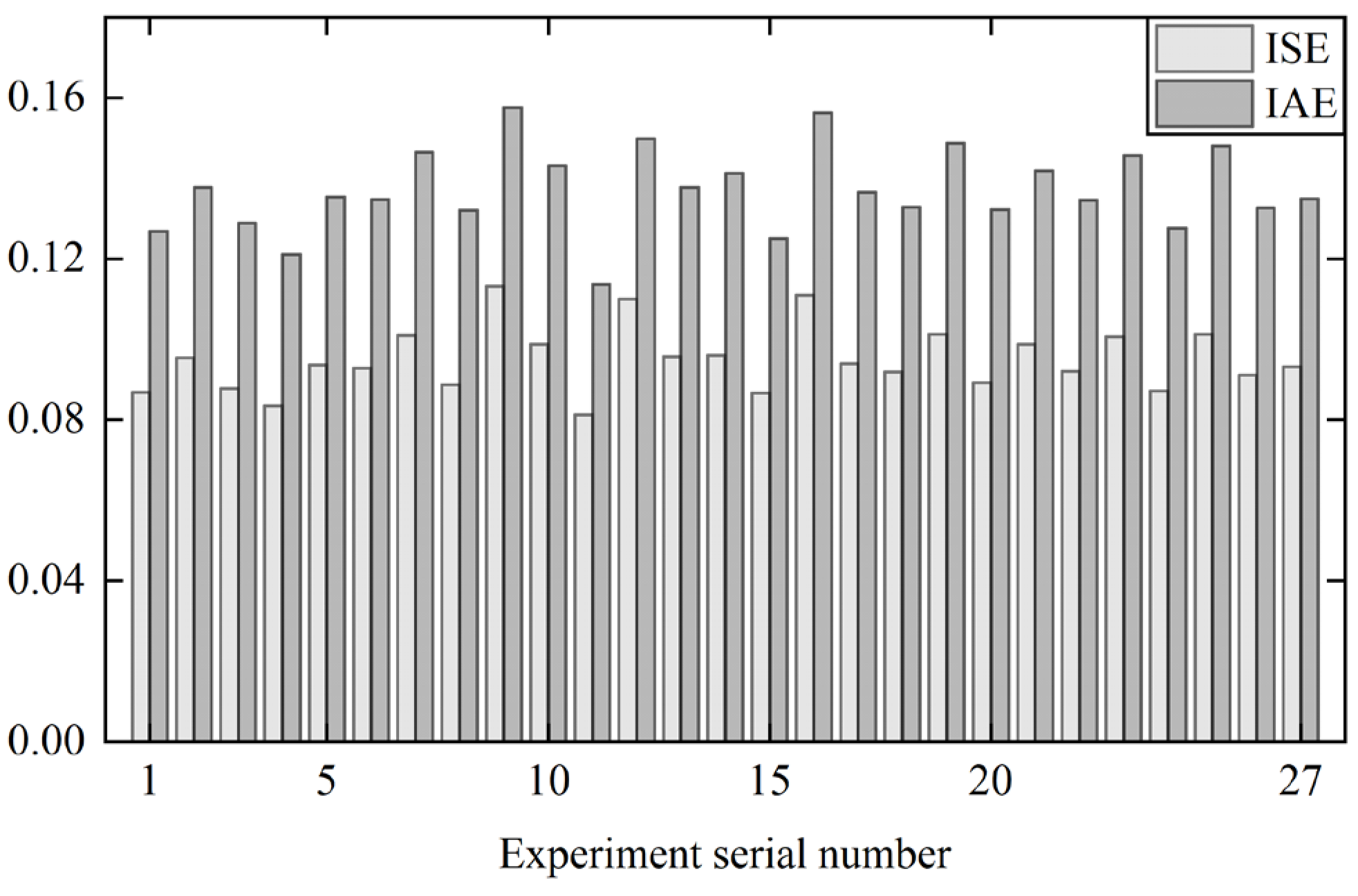
First, the optimal hyperparameter combination for each loop of the reinforcement learning control system is determined through orthogonal experiments. Based on experience, the learning rate is set at three levels: 0.001, 0.01, and 0.02; the discount factor is set at three levels: 0.90, 0.95, and 0.99. The number of hidden layer center nodes and their positions in the RBF network are determined using the OPTICS algorithm. This algorithm performs clustering analysis on the input data, effectively identifying the appropriate center points and the number of nodes. Based on the optimization results from the OPTICS algorithm, the network’s topology is determined to be 3-8-4. The experimental design is shown in

Table 8. Orthogonal table of hyperparameters for the primary airflow PI control system.

Experiment Number	${\mathit{\eta }}^{\prime }$	${\mathit{\eta }}^{″}$	${\mathit{\eta }}_{\mathit{c}}$	${\mathit{\eta }}_{\mathit{\sigma }}$	$\mathit{\gamma }$
1	0.001	0.001	0.001	0.001	0.9
2	0.001	0.001	0.01	0.01	0.95
3	0.001	0.001	0.02	0.02	0.99
⋮	⋮	⋮	⋮	⋮	⋮
26	0.02	0.02	0.01	0.001	0.99
27	0.02	0.02	0.02	0.01	0.9

, using the standard L₍₂₇₎(3¹³) orthogonal table for combination design. A total of 100 groups are randomly selected from the dataset for the experiment, and the ISE and IAE are used as evaluation metrics. Figure 18 shows the experimental results of various hyperparameter combinations for the primary airflow PI control system. It can be observed that Experiment Group 11 performs the best.

Table 9. Hyperparameter settings for reinforcement learning in each control loop.

	${\mathit{\eta }}^{\prime }$	${\mathit{\eta }}^{″}$	${\mathit{\eta }}_{\mathit{c}}$	${\mathit{\eta }}_{\mathit{\sigma }}$	$\mathit{\gamma }$
Primary airflow PI control loop	0.001	0.01	0.01	0.001	0.99
Secondary airflow PI control loop	0.001	0.01	0.001	0.001	0.95
Economizer feedwater flow PI control loop	0.001	0.02	0.01	0.001	0.95
Boiler drum pressure PI control loop	0.001	0.01	0.001	0.02	0.99
Secondary fan outlet air pressure PI control loop	0.001	0.001	0.02	0.001	0.9

presents the optimal hyperparameter combinations for all sub-loop PI control systems obtained through the orthogonal experiment.

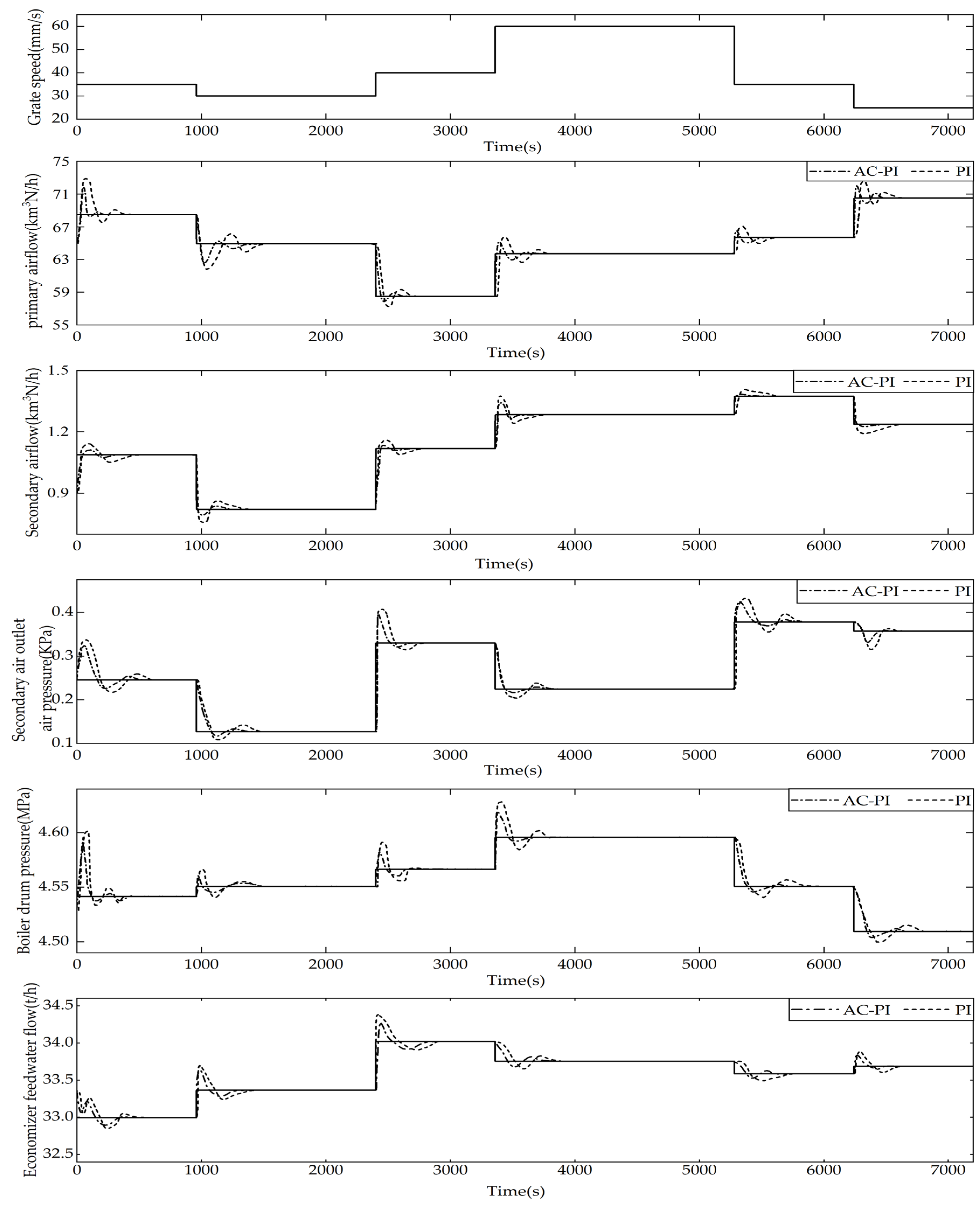
Figure 19 shows that when the grate speed changes, the optimization setting module of manipulated variables based on IALO can recognize the change in operating conditions and automatically updates the setting values of the manipulated variables ($S_1–S_5$) to better fit the changed conditions. The updated setting values are then sent to the reinforcement learning-based PI MSFR control system to execute the new setting values.

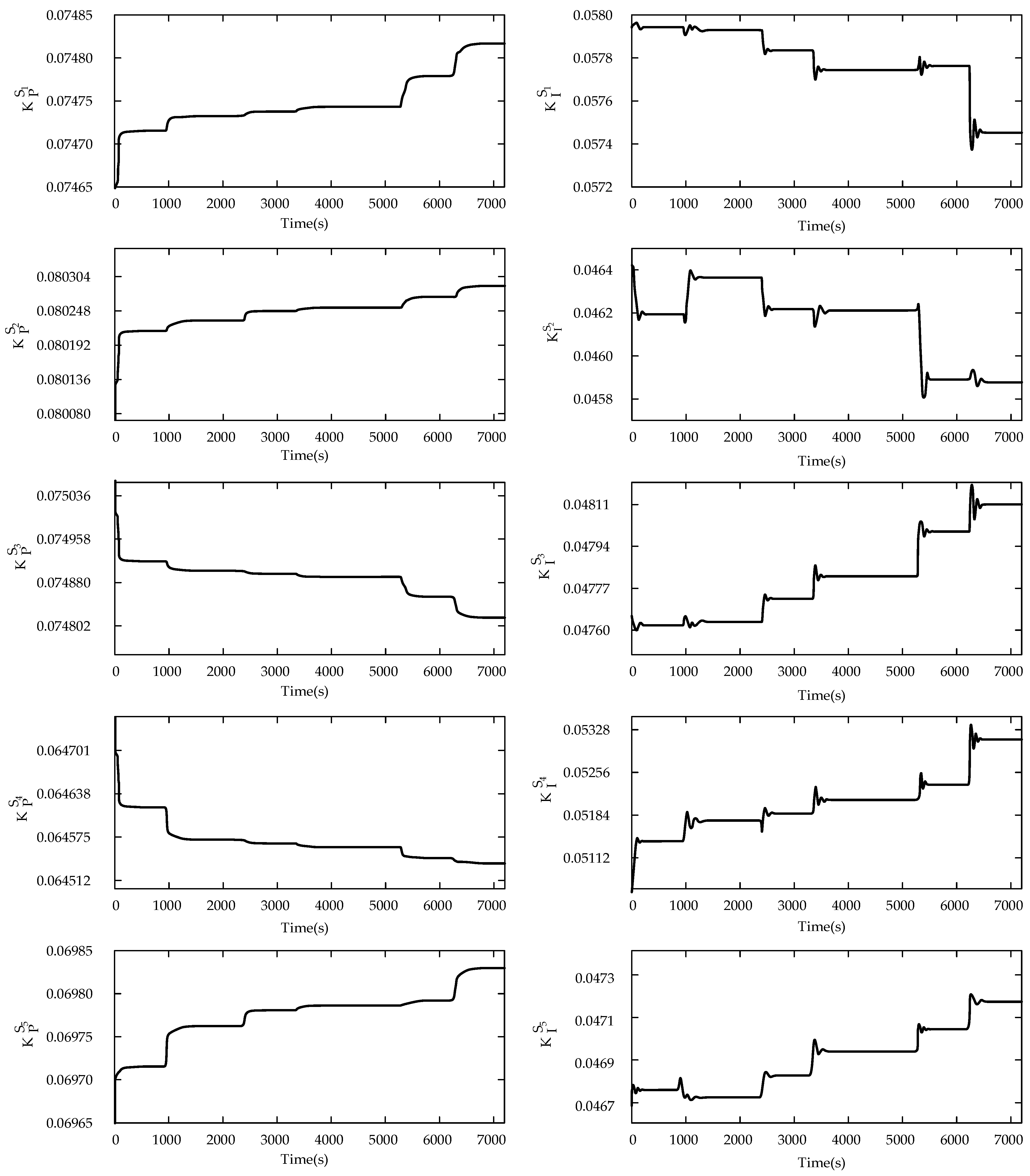
The loop control system automatically tunes the PI parameters according to the changed operating conditions, enabling rapid tracking of the updated manipulated variables settings. Figure 20 shows the process of adaptive adjustment of PI parameters in the AC-PI control system, and

Table 10. The setpoint of the PI parameters in the PI control system.

	KP	KI
Primary airflow PI control loop	0.07472	0.05774
Secondary airflow PI control loop	0.08019	0.04623
Economizer feedwater flow PI control loop	0.07488	0.04777
Boiler drum pressure PI control loop	0.06457	0.05184
Secondary fan outlet air pressure PI control loop	0.06975	0.04693

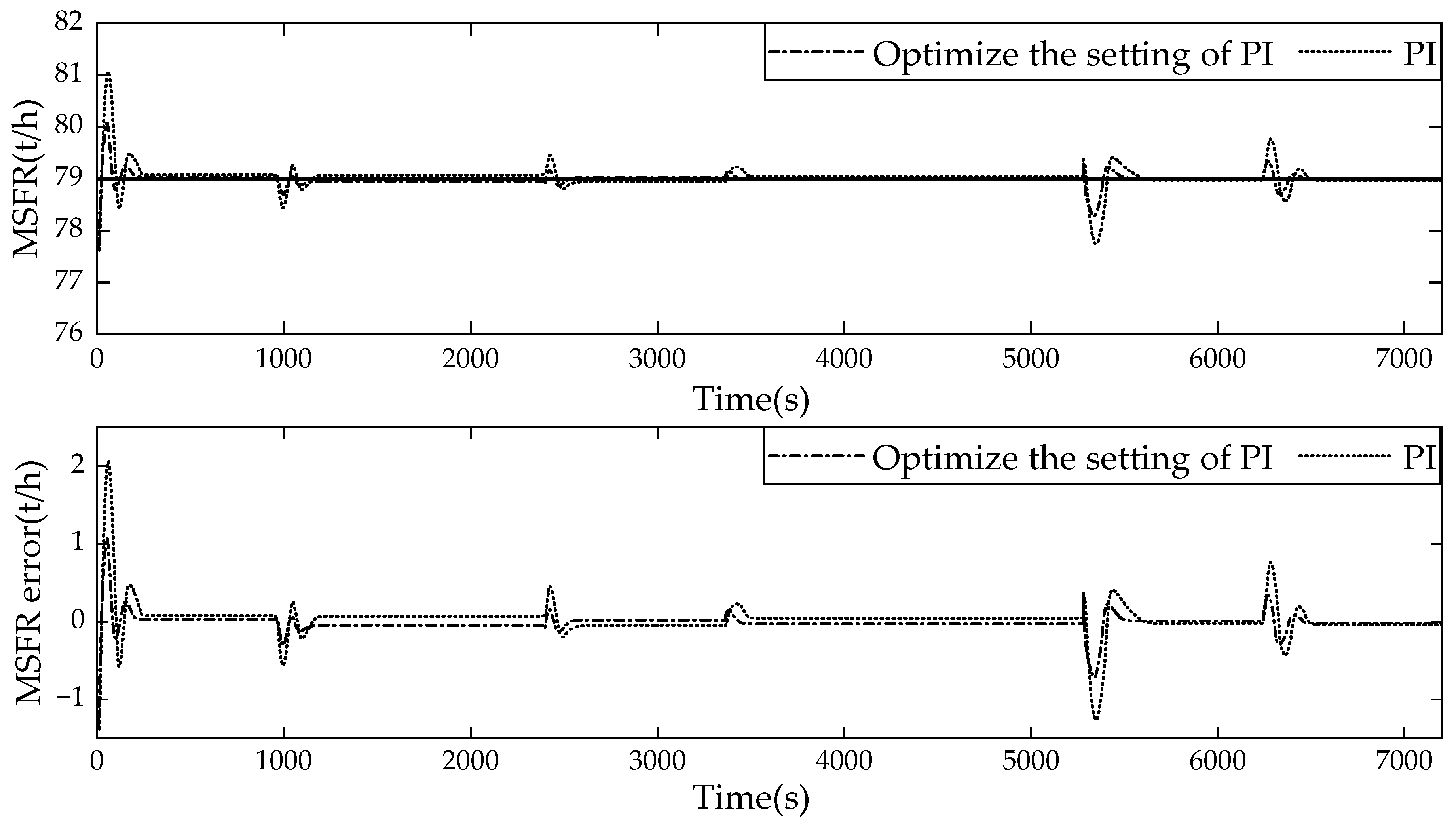
lists the PI setpoints of the PI control system. The actual manipulated variables of the control system are then sent to the object model of the MSFR in the MSWI process [44], and the controlled MSFR results are shown in Figure 21. It can be seen that, compared to traditional PI methods, the intelligent control method proposed in this article can control the MSFR within the target range.

Table 11. Evaluation of the effectiveness of control of MSFR.

	ISE	IAE	DEVmax	$\overline{\mathit{\sigma }}\mathit{\%}$	${\overline{\mathit{t}}}_{\mathit{r}}$ (s)	${\overline{\mathit{t}}}_{\mathit{s}}$ (s)
Optimize the setting of PID	0.0671	0.0882	3.2901	1.43%	48.21	421.69
PID	0.0823	0.0988	3.4632	1.69%	46.23	445.41
QDRNN-PID	0.0716	0.0931	3.3772	1.51%	50.50	444.67
PID	0.1074	0.1130	3.5592	1.84%	46.83	475.83

shows the compared results with traditional PID methods, such as QDRNN-PID from the literature [44]. The comparison is evaluated based on integral square error (ISE), absolute error integral (AIE), maximum deviation, average quantization overshoot, average rise time, and average response time. It can be seen that the proposed method demonstrates good transient response, stability, and anti-interference ability, showing superior performance.

4.4. Comprehensive Analysis

The experimental results show that when the grate speed changes, indicating a shift in the operating conditions of the solid waste incineration process, the proposed method effectively detects these changes and re-optimizes the key control variables (such as primary airflow, secondary airflow, secondary fan outlet air pressure, boiler drum pressure, and economizer feedwater flow). By employing the IALO method, the system can rapidly optimize the setpoints of the control variables based on the target MSFR, ensuring alignment with the current operating conditions. The loop control layer then implements the new optimized setpoints. In the loop control layer, the PI controller parameters can be dynamically adjusted in response to changing operating conditions. Experimental results demonstrate that when the working operating conditions change, the optimized setpoints are recalibrated accordingly, and the control loop can quickly track the new setpoints, thereby maintaining the MSFR within the target range.

5. Conclusions

The MSFR in the MSWI process is one of the key factors for the stable operation of the incineration system. Due to its strong coupling, nonlinearity, and multivariable nature, effectively controlling the MSFR presents significant challenges. To address the control needs of the MSWI process’s MSFR, a two-layer intelligent control method is proposed, consisting of an optimization setting layer and a loop control layer. This method can adaptively adjust the setpoints of key manipulated variables under varying operating conditions. The loop control system then implements these setpoints, ultimately ensuring that the MSFR is controlled within the target range. Simulations based on industrial sample data collected from the field were conducted to verify the effectiveness of the proposed method.

Although this study has made progress in the control strategy for MSFR, several issues require further attention. For example, the two-layer structure control method used in this paper helps alleviate the computational burden by distributing algorithms across different devices. However, it inevitably increases computational costs. The system is also highly sensitive to sensor noise, which can interfere with data collection and affect control decisions. This issue is particularly significant in developing countries, where computational resources are limited and may become more pronounced.

Additionally, there is a lack of systematic research on the trade-offs between energy recovery and toxic emissions (e.g., dioxins). This gap arises mainly from the asymmetry of monitoring data—high-frequency energy recovery data and low-frequency dioxin sampling data are difficult to correlate effectively.

Future research will involve empirical experiments in collaboration with industry partners. The goal is to develop a multi-objective optimization model that provides innovative solutions for achieving energy-environmental synergy. Moreover, another important aspect is balancing MSFR stability with emission control. Future studies could focus on developing a multi-objective function that integrates both MSFR stability and emission control. This approach would optimize both the control accuracy of the MSFR and emission control, offering a more comprehensive and effective solution.