Abstract
Ensuring the resilient navigation of unmanned aerial vehicles (UAVs) under conditions of limited or unstable sensor information is one of the key challenges of modern autonomous mobility within smart infrastructure and sustainable development. This article proposes an intelligent autonomous UAV control method based on the integration of geometric trajectory modeling, neural network-based sensor data filtering, and reinforcement learning. The geometric model, constructed using path coordinates, allows the trajectory tracking problem to be formalized as an affine control system, which ensures motion stability even in cases of partial data loss. To process noisy or fragmented GPS and IMU signals, an LSTM-based recurrent neural network filter is implemented. This significantly reduces positioning errors and maintains trajectory stability under environmental disturbances. In addition, the navigation system includes a reinforcement learning module that performs real-time obstacle prediction, path correction, and speed adaptation. The method has been tested in a simulated environment with limited sensor availability, variable velocity profiles, and dynamic obstacles. The results confirm the functionality and effectiveness of the proposed navigation system under sensor-deficient conditions. The approach is applicable to environmental monitoring, autonomous delivery, precision agriculture, and emergency response missions within smart regions. Its implementation contributes to achieving the Sustainable Development Goals (SDG 9, SDG 11, and SDG 13) by enhancing autonomy, energy efficiency, and the safety of flight operations.
1. Introduction
1.1. Motivation
For autonomous UAV control under conditions of visual data deficiency, the task of trajectory tracking becomes especially important. Limited environmental information requires UAVs to follow a given path precisely and reliably, minimizing deviations even in the absence of full situational awareness. In such scenarios, path stabilization and intelligent obstacle avoidance are interrelated and critical for mission success.
Traditional trajectory tracking approaches, such as pure pursuit, line-of-sight (LOS), and vector field methods, are effective when sufficient environmental data are available. However, under conditions of visual degradation—such as poor lighting or external obstructions—these approaches fail to provide stable path adherence. More promising methods involve nonlinear stabilization techniques, where the system of motion equations is transformed into a quasi-canonical form. This allows the control problem to be reformulated as an inverse dynamics task, providing more reliable trajectory tracking in dynamic and uncertain conditions.
Trajectory tracking under limited information is essentially an intelligent control problem, where UAV position must be stabilized relative to the path using adaptive algorithms that account for incomplete or inaccurate sensor inputs. The use of path coordinates enables the real-time estimation of trajectory deviation, which is critical for rapid course correction. These coordinates represent state variables that describe the UAV’s position relative to a target point on the path. For bidirectional control, the system can select the nearest target point to the UAV’s current position. This approach is especially effective in two-dimensional spaces, where deviations can be expressed in two parameters. In three-dimensional environments, the concept of path coordinates is also applicable, although it requires more complex stabilization algorithms.
Intelligent motion control methods based on quasi-canonical forms and normal form theory allow for the synthesis of control strategies that not only stabilize the trajectory but also adapt to limited visibility conditions. This opens the possibility of building control systems that adaptively regulate velocity and heading, minimizing trajectory deviation even as environmental conditions change.
This paper develops a novel method of intelligent UAV motion control under visual data deficiency. The proposed approach uniquely combines geometric path tracking, LSTM-based sensor filtering, and reinforcement learning (RL) for adaptive speed and obstacle avoidance. Unlike classical methods relying solely on GPS/IMU or fixed controllers, our method maintains trajectory stability even under signal degradation. Simulation results show that trajectory deviation is reduced by up to 70% and GPS error is filtered by a factor of 3–5 compared to raw data. These quantifiable gains highlight the system’s ability to ensure resilient navigation and energy-efficient control under uncertain conditions.
A structural diagram of the proposed method is shown in Figure 1.
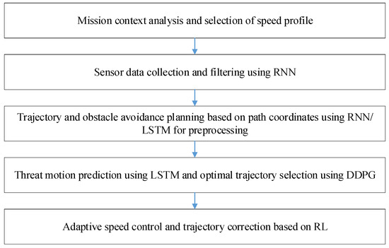
Figure 1.
Structural diagram of the intelligent autonomous UAV motion control method under visual data deficiency.
At the first stage, the mission objective (e.g., monitoring, reconnaissance, cargo delivery, or hybrid task) is analyzed to determine avoidance priorities. Based on the selected objective, a motion profile is formed. Then, an AI-based algorithm selects an appropriate speed profile, prioritizing either safety or efficiency. Depending on the mission goal, obstacle avoidance parameters are defined, such as sensitivity to obstacles, allowable course deviation, and speed thresholds. A reinforcement learning (RL) module tunes the avoidance parameters based on mission complexity and environmental conditions.
At the second stage, data about the location of nearby obstacles are collected using available sensors such as lidars, ultrasonic sensors, and radar systems. Recurrent neural networks (RNNs) are used for the sequential processing of sensor inputs, including obstacle density analysis, distance estimation, and real-time threat map generation.
In the third stage, alternative avoidance trajectories are formed. Path coordinates are used to construct trajectories that provide safe obstacle avoidance. RNNs or LSTM networks generate predicted avoidance paths based on sensor data by analyzing sequential inputs to anticipate UAV motion in the current conditions. Based on the collected data and constructed trajectories, a threat map is generated, highlighting critical zones around the UAV that require avoidance.
One essential component of the proposed intelligent control method is obstacle motion prediction and avoidance planning at the fourth stage. Using sensor data and prior states, the system estimates the most probable trajectories of moving objects. The application of Bishop frame theory allows the avoidance trajectory to be designed and adapted to the 3D environment and the positions of dynamic obstacles.
Machine learning methods are used to predict the future positions of moving threats by analyzing sequential changes in sensor data. The algorithm then selects the safest trajectory that bypasses the threat while minimizing deviation from the original route.
At the fifth stage, the speed profile along the avoidance trajectory is adaptively adjusted. The UAV’s velocity is modified depending on the obstacle density and proximity to threats. Machine learning algorithms manage real-time speed control, adjusting it based on current environmental conditions and risk level. As the UAV approaches a high-risk zone, speed is reduced to enhance maneuverability.
Thus, path coordinates, speed profiles, and trajectory stabilization data are used at every stage, while machine learning reinforces the system’s avoidance capability through prediction, adaptation to environmental changes, and dynamic control.
1.2. State of the Art
Given the complexity of autonomous UAV navigation tasks under conditions of incomplete or noisy information, it is appropriate to review the literature by stages of the system’s functioning: from mission context definition to sensor data filtering, obstacle avoidance, trajectory prediction, and adaptive control. This breakdown allows for a critical analysis of existing approaches and highlights gaps that form the basis of our methodology.
Analytical reviews. In recent years, there has been a growing body of research on the use of UAVs in the infrastructure of smart regions. Studies [1,2,3] provide a comprehensive overview of the main directions of drone applications in environmental monitoring, emergency logistics, agriculture, energy, and urban infrastructure management. These reviews emphasize the significant potential of UAVs in achieving the Sustainable Development Goals—namely SDG 9, 11, and 13 [4].
The authors of [1] underline the importance of developing adaptive architectures capable of functioning under conditions of sensor data scarcity. In [2], the limited autonomy and resilience of current solutions are emphasized. Review [3] summarizes the technological capabilities of UAVs while identifying key limitations, such as scalability issues, real-time data processing challenges, sensitivity to weather conditions, and insufficient adaptability.
Publications [5,6] highlight the lack of a unified system architecture that would integrate artificial intelligence, neural network-based filtering, and adaptive control in unstable environments.
Mission context and speed profile selection. Study [7] explores the use of fuzzy logic to support navigation decisions under uncertain inputs (e.g., lighting, object velocity, and obstacle distance). Although effective in stable conditions, this method fails under abrupt GPS changes and neglects dynamic obstacles. In [8], dynamic speed control is implemented via fuzzy regulators, yet the absence of scenario variability analysis limits applicability in dynamic environments.
Thus, fuzzy systems are flexible but do not scale well without forecasting or self-learning mechanisms.
Sensor data filtering using RNNs. In [9], an RNN-based filter is proposed for GPS drift compensation, though testing was limited to short (2 min) simulated data. In [10], LSTM filtering is applied to IMU signals, but the method is designed for FOG-IMUs, limiting its applicability to multirotor UAVs using MEMS sensors. In [11], LSTM outperformed Kalman filtering in urban scenarios; however, multi-sensor integration was not considered.
It can be concluded that RNN-based filters show potential but require extension to multi-sensor configurations and more realistic deployment scenarios.
Trajectory generation using path coordinates. Studies [12,13] introduce geometric transformations into path coordinates to formalize obstacle avoidance as an affine control problem. However, they do not evaluate scalability for scenarios with multiple obstacles. In [14], dynamic adaptation of coordinates is proposed, yet its high computational complexity limits use on low-power UAVs.
Thus, geometric models are useful but not inherently adaptive to unpredictable environments without AI support.
Trajectory prediction and optimization using reinforcement learning. DDPG and PPO algorithms were applied in [15] to perform obstacle avoidance in simulation. However, testing was limited to short episodes (up to 60 s) without accounting for real-world noise or wind. Study [16] introduces risk assessment via neural networks, but the system is highly sensitive to the accuracy of the dynamics model and is difficult to transfer from simulation to physical UAVs.
We conclude that reinforcement learning holds significant potential, but greater robustness to unexpected situations and unstable inputs is needed.
Adaptive speed control using RL. Study [17] shows that an RL agent can adapt the UAV’s speed and reduce energy consumption by 15–20%. However, latency in decision making and limited cooperation with PID regulators are noted. In [18], the authors emphasize the benefits of speed profile adaptation, but the model’s complexity restricts practical implementation. In [19], a hybrid model combining FNN and fuzzy logic improves interpretability but is designed exclusively for fixed-wing UAVs.
These studies suggest that existing systems are partially adaptive but require improvement in energy efficiency and broader applicability.
Most reviewed approaches focus on isolated aspects of the problem—filtering, avoidance, or adaptation. Meanwhile:
- −
- there is a lack of integrated architectures combining AI-based filtering, geometric planning, and RL-based trajectory prediction;
- −
- most models are trained and tested in simulation, without consideration for sensor degradation or visual data loss;
- −
- the relationship between technical autonomy and sustainable development goals is largely overlooked.
Therefore, the problem of the intelligent assurance of resilient UAV navigation under visual data deficiency remains highly relevant. The system proposed in this paper:
- −
- adapts to sensor information loss,
- −
- predicts and stabilizes UAV trajectory in real time,
- −
- ensures energy-efficient and safe UAV operation in smart region environments.
1.3. Objectives and Contribution
The aim of this study is to develop a method for resilient UAV navigation under conditions of limited visual information by integrating geometric control theory, recurrent neural network (RNN)-based filtering, and reinforcement learning (RL). The proposed solution is intended to ensure adaptive motion control for UAVs operating in smart region environments where sensor data are noisy, fragmented, or unstable.
This article presents a structured review of existing autonomous UAV navigation methods under low-visibility conditions. Based on the review, a scientific problem was identified: the absence of a unified architecture that integrates predictive data filtering, geometric trajectory tracking, and adaptive control using reinforcement learning in scenarios with partial or missing sensor inputs.
The proposed method implements a hybrid control approach that uses the Frenet–Serret coordinate system and affine system stabilization to enable reliable path tracking even under perturbed GPS or IMU signals. The RNN-based model performs the filtering and compensation of sensor noise, while the RL module provides real-time risk prediction, obstacle avoidance, and speed adaptation. Simulation experiments incorporating variable velocity profiles, lateral wind, and signal delays demonstrate the robustness and effectiveness of the proposed system.
A key feature of the proposed approach is the integration of RNN-based filtering with RL-based decision making, which enables robust navigation performance under information uncertainty and degraded visibility. In contrast to conventional systems that rely on full sensor availability or visual localization, the developed method ensures stable trajectory tracking under conditions of sensor data deficiency.
2. Materials and Methods
2.1. The Role of Resilient UAV Navigation in Enabling Mobile Solutions for Smart Regions
With the ongoing trend of urbanization and the rising demand for infrastructure efficiency in smart cities, mobile autonomous systems are gaining increasing importance as essential tools for achieving the Sustainable Development Goals (SDGs) [4]. As noted in recent systematic reviews [20], autonomous mobility technologies offer effective solutions for complex challenges in both urban and regional environments, characterized by varying risk levels, resource constraints, and diverse societal requirements.
Among the most versatile and rapidly evolving types of such systems are unmanned aerial vehicles (UAVs). These platforms are compact, flexible, and energy-efficient, enabling reliable operation in remote or hazardous areas. The development and deployment of UAV technologies contribute directly to the advancement of SDG 9 (industry, innovation, and infrastructure), SDG 11 (sustainable cities and communities), and SDG 13 (climate action).
Thanks to their autonomy and low dependence on ground-based infrastructure, UAVs are increasingly being utilized in smart regions for a wide range of applications. These include environmental monitoring—such as the assessment of soil quality, emission levels, and forest health—autonomous logistics involving the delivery of medical supplies to inaccessible areas, infrastructure inspection tasks focusing on power lines, rooftops, and bridges, emergency response operations that involve locating victims, transporting medical equipment, or assessing fire zones, as well as precision agriculture, where UAVs are used for aerial imaging, pest identification, and moisture analysis.
These applications not only increase operational efficiency in critical sectors but also contribute to reduced environmental impact, decreased fuel use, enhanced human safety, and more efficient resource utilization.
However, to enable the large-scale integration of UAVs into the sustainable infrastructure of smart regions, it is essential to ensure their resilient autonomy—the ability to navigate and make decisions under uncertainty without human intervention or complete sensor input. This challenge forms the foundation of our research.
Despite the growing use of UAVs in sustainability-focused missions, autonomous navigation remains a significant engineering and scientific challenge, particularly in unstructured or visually constrained environments. Most commercial and research-grade UAV systems rely on sensor suites such as GPS, inertial measurement units (IMUs), cameras, and lidars to navigate. However, in real-world settings, these sources are often unreliable or unavailable.
Under conditions like dense fog, rain, snow, smoke, dust, or darkness, visual sensors become ineffective, limiting the capabilities of computer vision and obstacle recognition systems. As a result, traditional vision-based navigation or SLAM (Simultaneous Localization and Mapping) techniques are often non-functional.
In complex urban environments (urban canyon effect), dense forests, or areas with GPS jamming (such as disaster zones), positioning data may be inaccessible, delayed, or distorted, destabilizing the flight path.
Moreover, the real-world environment is rarely static. Side winds, turbulence, and shadow zones behind obstacles disrupt UAV trajectory. Traditional controllers like PID or MPC are often not equipped to handle such variability in real time and may require frequent parameter re-identification.
Another limitation is the computational cost of advanced navigation algorithms such as deep learning-based SLAM or multi-sensor fusion. Lightweight UAVs typically use low-power processors that cannot handle large-scale data in real time without latency.
Given these limitations, the concept of “resilient autonomy” has gained traction—referring to a UAV system’s ability not only to operate under ideal conditions but also to adapt, compensate for data loss, and maintain stability under uncertainty.
This concept extends beyond traditional approaches to trajectory stabilization. Within the framework of sustainable smart regions, resilient UAVs are expected to meet several critical requirements. They must be capable of adapting to fluctuations in sensor availability and data accuracy. Furthermore, they should possess the ability to make autonomous decisions regarding changes in motion strategy, including rerouting and obstacle avoidance. Another essential feature is the capacity to maintain energy efficiency by minimizing redundant corrections and unnecessary maneuvers. In addition, resilient UAVs should proactively forecast environmental conditions instead of relying solely on reactive responses. Lastly, they must be able to operate independently of centralized infrastructure, which is particularly important in the context of achieving SDG 9 and SDG 11.
From a technical standpoint, resilient autonomy integrates classical control methods (model-based control, kinematic planning) with artificial intelligence techniques (reinforcement learning, neural networks, fuzzy systems, hybrid AI). This combination allows systems to compensate for sensor failure, identify hidden dependencies, and maintain control even in visually degraded settings.
According to recent reviews [21], the fusion of autonomous reasoning and resilient behavior is a key driver of digital mobility aligned with sustainability. Smart regions that adopt such systems gain practical tools to implement scalable, safe, and intelligent services—from drone-based patrolling to autonomous deliveries in disaster areas.
In conclusion, the development of resilient intelligent navigation systems is not only technically justified but also socially and environmentally necessary. It enables the transformation of UAVs from limited-purpose tools into essential components of smart, sustainable regional mobility infrastructures.
Smart regions are not merely areas with digital infrastructure—they are ecosystems that integrate intelligent solutions to improve quality of life, optimize resource management, and increase resilience. Within this framework, resilient UAVs are mobile tools that support the sustainable functioning of territorial systems.
Thanks to their ability to operate autonomously even with limited sensor input, next-generation UAVs enable a wide range of new applications across multiple sustainability domains.
First, in the area of environmentally sustainable logistics (SDG 9 and SDG 13), UAVs support the delivery of medical supplies, vaccines, and blood samples to rural or isolated regions where road access is limited or nonexistent. They also help reduce CO2 emissions by substituting ground transportation in short- and medium-distance operations. Notable implementations of this include deliveries to remote areas in Africa and Asia, as well as emergency logistics during disaster relief missions.
Second, UAVs contribute significantly to environmental condition monitoring (SDG 13 and SDG 15). They are capable of detecting changes in forest structure, soil composition, and pollution levels in both air and water. Additionally, they are employed to monitor fires, floods, and hazardous material spills in low-visibility or inaccessible areas. Their resilient autonomy allows them to adjust trajectories in real time in response to environmental changes.
Third, in the context of infrastructure inspection (SDG 9 and SDG 11), UAVs can autonomously evaluate the condition of power lines, rooftops, bridges, and tunnels without the need for manual intervention. This function is especially valuable in post-disaster situations where conventional imagery is obstructed by smoke, debris, or damage. Their use minimizes human risk while improving the speed and quality of infrastructure assessments.
Fourth, for emergency response (SDG 11 and SDG 13), UAVs are deployed to survey disaster zones impacted by events such as earthquakes, wildfires, and floods. They assist with the real-time localization of victims and deliver critical supplies even in environments where GPS signals or visual data are unavailable. Their onboard processing capabilities enable rapid decision making, which is essential during the first-response window.
Finally, in precision agriculture and agri-analytics (SDG 2 and SDG 12), UAVs are used for field monitoring under various conditions, including nighttime or cloud cover, by relying on sensor networks that compensate for noise. They also facilitate the analysis of crop moisture, growth stages, and pest presence with minimal human involvement, thereby saving both time and operational resources.
Each of these use cases not only validates the practical utility of resilient UAVs but also highlights their strategic role in building smart-region ecosystems aligned with sustainability objectives. The integration of such systems contributes to infrastructural reliability, environmental accountability, and social inclusion—three pillars of SDG-oriented transformation.
These findings demonstrate that resilient UAV navigation is not only a technological challenge but also a strategic priority for shaping mobile infrastructure in smart, adaptive, and sustainable regions. In such regions, autonomous systems do not merely perform individual tasks—they form a cyber-physical platform that supports services in environmental protection, logistics, safety, inspection, and emergency response.
The defining factor for the success of such platforms is the ability of UAVs to function under informational uncertainty—without dependable GPS, camera data, or full situational awareness. In this context, there is a growing need for intelligent navigation methods that combine adaptability, prediction, and autonomy.
Developing such systems opens new possibilities for:
- −
- achieving the SDGs (9, 11, 13) through increased accessibility and reduced environmental impact;
- −
- integrating UAVs into digital mobility ecosystems, particularly in resource-constrained contexts;
- −
- moving beyond controlled autonomy toward true resilience-systems that not only follow predefined plans but also adapt in real time to the unknown.
Therefore, the objective of this article is to propose a UAV navigation approach that meets not only technical performance criteria but also the principles of sustainable, inclusive, and adaptive regional development. The following sections detail the methodological foundation, system architecture, test scenarios, and results that support its relevance in the context of smart regional transformation.
2.2. Technological Foundations
2.2.1. Mission Context Definition and Speed Profile Selection
The conversion from the normal coordinate system to the trajectory-aligned system can be described as a sequence of two rotational transformations
- −
- by angle ψ around the OYn axis counterclockwise, and then
- −
- by angle ζ around the new position of the OZn axis.
Based on the methodology outlined in [22], we construct the transformation vector basis from the trajectory frame back to the normal reference frame.
The rotation matrices are as follows:
The transformation matrix that converts coordinates from the normal system to the trajectory system is given by:
The set of vectors defining the transformation from the trajectory coordinate system to the normal coordinate system is structured as follows:
Accordingly:
From vectors (3) and expressions (4), the UAV’s motion as a material point can be characterized by its kinematic properties: position, velocity, and acceleration. The position is defined in 3D space by coordinates (x, y, z), velocity represents the rate and direction of movement, and acceleration reflects changes in velocity over time. The UAV’s velocity vector components in the normal coordinate system are:
The acceleration of a material point is the time differential of the vector (5):
The motion of the UAV as a material point is determined by its initial state and the sum of external forces represented by the coordinates Fx, Fy, and Fz in the Earth’s normal coordinate system. If the force vector is decomposed into the trajectory coordinate system, we obtain
According to Newton’s second law , F = ma, where m is the mass of the UAV, we can determine the position of the point in three-dimensional space as follows:
Among the external forces , gravity is distinguished as a non-controllable force, and the sum of other forces is referred to as the controllable force .
The magnitude of the gravitational force, i.e., the UAV’s weight, is expressed through its mass and the acceleration due to gravity. As a result, the gravitational force can be expressed in the Earth’s normal coordinate system as follows To convert it into the trajectory coordinate system, a corresponding transformation matrix is applied
The force vector normalized by the UAV’s weight is referred to as the load factor vector. This vector can be decomposed into two components: the projection onto the OXt axis and the projection onto the OYt plane. The first component is the longitudinal load factor vector; the second is the lateral load factor vector.
The longitudinal load factor is characterized by its coordinate along the nx axis, known as the longitudinal load factor. The lateral load factor is characterized by its magnitude ny, called the lateral load factor, and an inclination angle ζ, measured counterclockwise from the OXt axis.
The parameters nx, ny, and ζ fully define the controllable force and are considered control parameters in this model. The first parameter determines changes in the speed magnitude, while the second and third determine changes in the direction of velocity. The parameter ζ serves as an analog of the UAV’s body roll angle.
The force vector in the trajectory coordinate system, using the control parameters, can be written as:
Considering load factor-based force representation and the kinematic equations, the UAV’s motion is described by the following six differential equations:
Since system (9) is nonlinear in control inputs, it must be converted to an affine form for use in machine learning. This can be achieved through rotation, scaling, and shifting transformations. By applying the rotation method and introducing the variables v1 = nx, v2 = ny·cos(ζ), and v3 = ny·sin(ζ) as new virtual control elements, the following relationships can be derived:
The system (10) is transformed into an affine system with three control inputs.
When selecting a flight profile for a UAV, it is important to consider the specific features of the mission as well as the dynamic and operational limitations of the vehicle. The flight profile can be influenced by various factors: from the type of mission (monitoring, reconnaissance, cargo delivery) to the physical characteristics of the environment (presence of obstacles, altitude restrictions, etc.). At the same time, it is necessary to take into account the constraints imposed on the UAV’s dynamic characteristics.
These constraints relate to permissible values of state and control parameters. They depend on the UAV’s specific characteristics and are usually defined as a region of allowable flight conditions, commonly referred to as the “flight envelope.” This region specifies the bounds of feasible flight modes based on parameters such as altitude, speed, and load factor.
To simplify the problem, we assume that the constraints can be expressed in the form of fixed threshold values:
An important aspect is ensuring adherence to the prescribed trajectory, which enables effective task execution by minimizing deviation from the desired path.
2.2.2. Trajectory Tracking Model for Large Areas or Long-Distance Flights
One of the common scenarios involves performing monitoring and inspection tasks over large areas or long distances. In such cases, the trajectory is typically selected to lie in the horizontal plane at a fixed altitude, as this simplifies the control task and allows for more efficient use of the UAV’s resources. Accordingly, the problem is formulated as ensuring flight along a curve on a plane.
Flight within a horizontal plane implies a constant flight altitude, which can be written as h = const. Taking this into account, the system of Equation (10), which describes the UAV’s motion dynamics, is simplified and can be expressed in terms of the coordinates L, Z, V, ψ:
When moving in a plane at constant speed, the equation describing the change in the variable V can also be omitted, resulting in the following system of motion equations:
Here, V is a system parameter that has a constant value. Thus, the system of Equation (12) is affine with respect to the scalar control input v3.
It should be noted that due to the condition , the equality holds . This equality, along with the known value of v3 (where, ), allows for the unambiguous determination of the control inputs and , considering the additional constraint . This constraint is natural in trajectory tracking tasks.
Let be a planar curve with a natural parameter s, which describes the given trajectory in the plane. Let us choose , a specific point P on the curve that corresponds to a certain value of the parameter s. At this point P, we construct the accompanying basis of the curve, which consists of the unit tangent vector t and the normal vector n, forming a right-handed basis (see Figure 2).
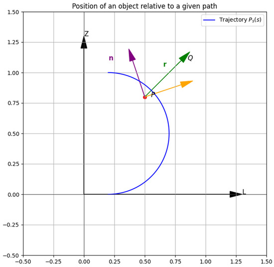
Figure 2.
Position of an object relative to a given path on a plane.
The position Q of the UAV’s center of mass can be related to point P by the formula:
where q is the radius vector of point Q; p is the radius vector of point P; r is the vector that connects point P with point Q.
q = p + r,
The vector r can be represented in the coordinates of the accompanying basis through e and d. Thus, according to Equation (13), we obtain the equality:
where
We differentiate this equation with respect to time, then:
Since , and for the tangent and normal vectors the following holds , where k is the curvature, we obtain:
After simplification, this equation can be written as:
This vector Equation (15) can be decomposed into components in the accompanying basis; to do this, it is sufficient to take the scalar product of the equation with the basis vectors. We obtain:
Thus, we find:
The quantities and represent the components of the velocity vector V in the accompanying basis. Let β be the angle of inclination of the vector V in the accompanying basis, then:
As a result, we obtain the dynamic equations in the coordinates of the accompanying basis:
The angle β can be expressed through two other angles: β = ψ − φc, where φc is the angle of inclination of the trajectory vector in the Earth-fixed (inertial) coordinate system. Differentiating this equation, we obtain:
Adding this equation to system (17), we obtain the equations of motion in the path coordinates e, d, β:
The control objective in system (18), which follows from the trajectory tracking problem, is to stabilize the variables e, d, and β at zero. However, the system contains another undefined parameter s, which is associated with the selection of a point on the curve considered as the target. It is also possible to use an additional control parameter that provides greater flexibility in the control law [23]. It is proposed to use the closest point on the curve as P, which is a common approach in trajectory tracking problems [24]. At the same time, this approach allows for the use of path coordinates only within a certain neighborhood of the curve. Specifically, this works when the trajectory curvature remains small, as coordinates are more stable to changes in such zones [25].
With the selected definition of the target point P, the condition e = 0 is satisfied, which implies that = 0. Thus, according to the first equation of system (18), we find:
Note that if > 0, the target point P moves along the trajectory in the positive direction (from the initial point of the curve to the final one) and if < 0, then in the negative direction. In theoretical analysis, it is sufficient to consider the case > 0, since changing the initial and final points allows the direction to be reversed. The chosen approach remains valid along the entire curve, as the condition 1 − kd > 0 must be met for the correctness of path coordinates. When this condition is satisfied, the sign of is determined by the angle β: if satisfies a specific condition, then > 0.
When choosing the target point P as the closest point on the curve, the parameter is determined by Formula (19), and the system of motion equations in path coordinates (18) takes the following form:
System (20) is defined on the set .
Thus, in the two-dimensional case of UAV motion along a given trajectory, the movement can be described by two parameters: the distance to the curve and the deviation angle between the velocity vector and the tangent vector of the curve at the closest point. If the stabilization of the variables e and d is achieved in system (20), the trajectory tracking problem for the UAV is solved.
In the case of UAV motion with constant speed, it is possible to consider solving the stabilization problem of the variables at zero for system (20) based on normal form theory. Let us choose variable d as the system output and construct the normal form of the system for this output. Assume:
Since cosβ ≠ 0 on the set D, the relative degree of system (20) is defined. The change of variables takes the form:
Under the condition , this change is invertible. In these variables, the system is written as:
where z = (z1,z2), and the variables k, d, β in this case are considered as functions of the variables z1, z2 which are defined by the change of variables.
The stabilizing control is chosen according to the formula:
The coefficients c1 and c2 should be selected so that the equation has negative roots.
The equation in system (21) describes the dynamics of the zero-dynamics system. In the case d = 0, β = 0 (i.e., when the UAV is stabilized on the trajectory), the equation simplifies to η = = V, which means that the UAV moves along the trajectory at constant speed.
When describing motion with non-constant speed, we may assume that the object’s speed is not constant. In this case, the task of defining the speed function V(t) becomes relevant. The system of Equation (20) then takes the form:
We choose z1 = d as the system output and define z2 = . Then:
If V(t) is a constant speed, substituting into the system yields the equation in normal form:
The stabilizing control is chosen in the case of constant speed as:
where the coefficients c1 and c2 should be chosen so that the equation has only negative roots.
It should be noted that the resulting control includes the derivative V′(t), which determines the rate of change of speed over time. In practice, the presence of V′(t) in the control law is often undesirable, and thus it becomes necessary to eliminate it. To achieve this, the control law can be modified to remove the dependence on V′(t). This is accomplished by introducing a new independent variable (instead of time).
For a system of the general form , the change of the independent variable is performed via the relation , where is a positive function. This substitution transforms the original system into the form:
where , and ξ should be considered a function of t, defined by the relation .
In our case, the change of the independent variable is performed as follows:
where ξ is the new independent variable.
With the new independent variable, system (23) transforms into the following:
We choose the output z1 = d. Then . Substituting s, we obtain the system in normal form:
and the control input v3 takes the form:
where c1 and c2 are coefficients that affect the stability of the motion and ensure that the variables d and β converge to zero, thereby solving the trajectory tracking problem with non-constant speed V(t).
2.2.3. Study of the Trajectory Tracking Model over Large Areas or Long Distances
We will conduct a study of the developed trajectory tracking model for large areas or long distances. To achieve this, we will develop a code using the Python 3.13.3 programming language. This code is intended to simulate UAV motion along various trajectories, such as a straight line, a circle, and a spiral. The code includes the following key components:
- −
- path—defines different types of trajectories (straight, circular, spiral);
- −
- UAV—simulates UAV motion considering deviations and control inputs;
- −
- visualizer—responsible for visualizing trajectories, deviations, and control inputs.
Several trajectory scenarios were selected for the analysis, imitating UAV motion over large areas or long distances. The trajectories include:
- −
- straight line—modeled as simple motion over long segments with constant or variable speed;
- −
- circular trajectory—represents typical monitoring tasks (e.g., observing objects at a fixed distance).
For each scenario, the specific features of the trajectories were taken into account, and a regulated control model was applied to minimize deviations.
The simulation was conducted under the following conditions:
- −
- a straight trajectory with an initial point P0 = [0,0] and a final point Pf = [400,400];
- −
- a circular trajectory defined by center O = [0,0] and radius r = 80;
- −
- a piecewise linear trajectory formed by connecting segments between the vertices [10,0], [13,−2,0], [15,3,0] using the Dubins path method [26];
- −
- a spiral trajectory described by the equations x = cos(t), y = sin(t), z = t/(2π).
To test the stabilizing properties of the control method, the initial UAV position was set as Q0 = [100,0] with a deviation from the trajectory. The control gain coefficients were selected as c1 = 0.035 and c2 = 1.95.
The simulation scenarios were divided into two main cases:
Trajectory tracking with constant speed—in this case, the speed was V = 5 m/s, and the initial heading angle ψ0 = 0;
Trajectory tracking with variable speed—for this case, a speed profile was used:
Figure 3 shows the implementation of Scenario 1 (straight trajectory with constant speed).

Figure 3.
Visual representation of the implementation of Scenario 1 (straight trajectory with constant speed).
For the simulation of motion along a straight trajectory, a constant speed of V = 5 m/s was selected. The initial position of the UAV was offset from the trajectory, allowing us to evaluate the effectiveness of control stabilization.
The dashed line in this figure indicates the ideal trajectory that the UAV is intended to follow. In this case, it is a straight line defined as the target. The solid line represents the actual UAV path. It begins from an initial point that has a significant deviation from the target trajectory and demonstrates how the control system corrects the UAV’s motion to align with the ideal trajectory.
The control system demonstrated high efficiency in stabilizing the motion. The maximum deviation quickly decreases to zero, and the UAV begins to follow the straight line accurately.
This result confirms the model’s ability to rapidly correct the trajectory, even in the presence of significant initial deviation.
The experimental results are presented in Figure 4 as a graph. It shows how the deviations from the target trajectory in the X and Y coordinates change over time. As seen from the graph, the deviation in X (blue line) initially increases rapidly, corresponding to movement toward the trajectory, but gradually decreases to zero.
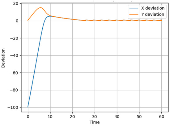
Figure 4.
Graph showing the change in UAV deviation from the desired trajectory in X and Y coordinates over time during the implementation of Scenario 1.
The deviation in Y (orange line) also starts at a certain value and gradually stabilizes at zero.
Thus, the figure demonstrates the effectiveness of the presented model: the system stabilizes the UAV, reducing the deviation to zero.
Figure 5 presents the circular trajectory that the UAV is expected to follow. The dashed line (Path) represents the ideal route in the form of a circle, while the solid line (UAV trajectory) shows the actual path taken by the UAV.

Figure 5.
Visual representation of scenario 2 (circular trajectory with constant speed).
As can be seen from Figure 5, the initial position of the UAV is outside the circular trajectory. During the flight, the UAV adjusts its position, gradually reducing the deviation from the assigned path.
The final result shows that the UAV trajectory converges to the desired circle with a radius of approximately 80 m. This confirms that the control system ensures the UAV follows the circular path despite the initial deviation.
This interleaved pattern observed in the deviation plots along the X and Y axes (Figure 6) can be explained by the geometry of the circular trajectory and the control law derived in the Frenet–Serret frame. According to the system of equations:
the deviation in the normal direction (denoted as d) evolves based on the sine of the deviation angle β, while the longitudinal deviation e is affected by the cosine term. For circular trajectories, the curvature k(s) is nonzero and constant, which introduces periodic dynamics in , thereby influencing both e and d. Since β oscillates over time, this leads to the phase-shifted (interleaved) sinusoidal behavior of deviations in the X and Y coordinates observed in the plots. In other words, as the UAV corrects its course along a circular path, the projections of the deviation on the X and Y axes fluctuate with a phase difference due to the rotational symmetry and curvature-induced dynamics. This behavior is consistent with the theoretical model and validates the fidelity of the trajectory-following algorithm.
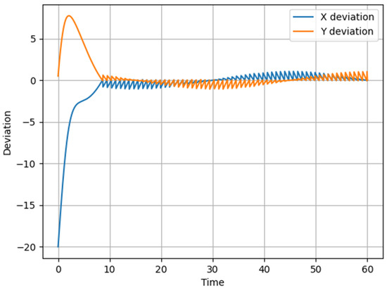
Figure 6.
Graph of UAV deviation in X and Y coordinates relative to the specified circular trajectory over time during the implementation of Scenario 2.
Figure 6 shows the graph of UAV deviation in X and Y coordinates relative to the assigned circular trajectory over time.
The deviations in X (blue line) and Y (orange line) exhibit a harmonic pattern. In the initial stages (0–10 s), the deviation increases sharply. This is due to the UAV not yet having adapted to the specified trajectory. After this phase, the system stabilizes, and the deviation gradually decreases, approaching zero. A slight wave-like behavior of the deviations is observed after 20 s, indicating trajectory correction due to control actions. Thus, both components of the deviation oscillate with a gradual decrease in amplitude, reflecting the process of UAV position stabilization. The oscillations are caused by the circular nature of the trajectory, as the control system continuously adjusts the heading.
The deviations show how the control system responds to the initial error, gradually aligning the trajectory. The result indicates the stability of the control system.
Thus, the visual representation of Scenario 2 illustrates the UAV’s spatial behavior, while the deviation graph details how the control system reduces errors in the X and Y coordinates. The reduction in the amplitude of oscillations on the deviation graph corresponds to the convergence of the actual UAV trajectory to the target circle in the first graph. These results demonstrate the relationship between spatial motion and the trajectory stabilization process.
The three-dimensional graph shown in Figure 7 visualizes the UAV’s trajectory as it follows a straight-line path with variable speed. As in previous cases, the ideal reference trajectory (Path) is indicated by the dashed blue line, while the actual UAV trajectory is shown as a solid orange line (UAV trajectory).
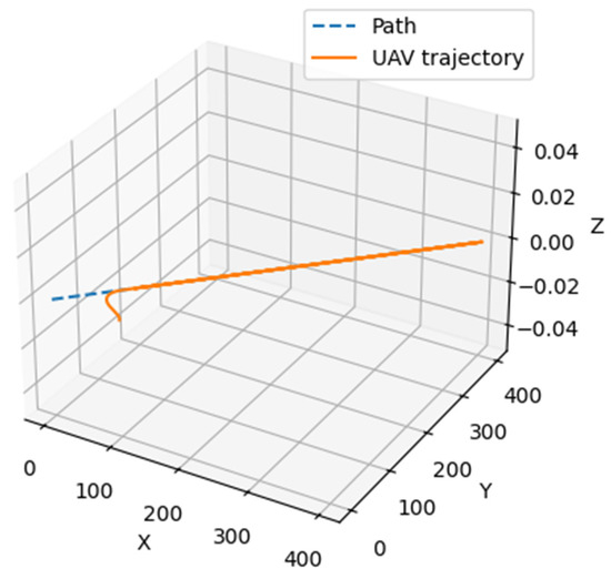
Figure 7.
Visual representation of the implementation of Scenario 3 (straight trajectory with variable speed).
The initial phase of motion shows a deviation from the assigned trajectory, which is explained by the inertia of the control system, the need to correct initial conditions, and the tuning of control inputs.
After the transient phase, a gradual decrease in deviations occurs, indicating the effectiveness of the trajectory correction algorithm. The Z-axis value remains practically unchanged, indicating no influence of vertical oscillations in the model.
It is important to note that the final part of the trajectory demonstrates stable straight-line following, indicating adaptation by the control system. The model parameters remained constant throughout. The trajectory length is approximately 400 m, and the control coefficients are: c1 = 0.035, c2 = 1.95. The speed function takes into account initial acceleration, a stabilization phase, and possible deceleration.
The graph in Figure 8 shows the deviation changes from the reference straight-line trajectory over time. The blue line represents deviation along the X-axis, and the orange line represents deviation along the Y-axis.
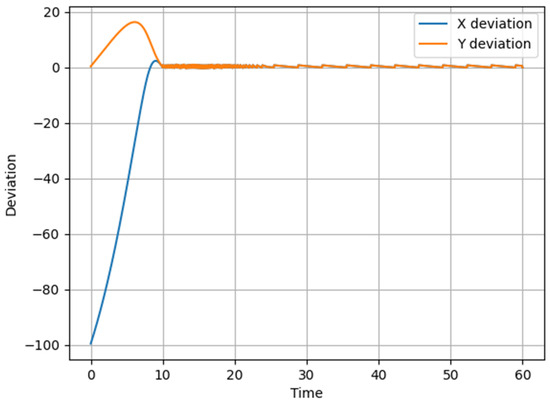
Figure 8.
Graph of UAV deviation in X and Y coordinates relative to the assigned circular trajectory over time during the implementation of Scenario 3.
In the initial stage (first 10 s), a significant increase in deviations is observed, especially along the X-axis, which is associated with control delay effects due to the initial dynamic conditions.
The deviation along the Y-axis also initially increases but then demonstrates stabilization, indicating the tuning of the control algorithm to compensate for the deviations.
After 10–15 s, the system reaches a steady-state mode in which the deviations decrease and remain within acceptable limits. The presence of slight oscillations in the final phase is explained by the behavior of the correction algorithm, which attempts to minimize error but exhibits small fluctuations.
The control profile effectively compensates for the initial deviations, although the system experiences a transient phase. Achieving a steady-state condition around X ≈ −5 m and Y ≈ 2 m indicates the operation of the stabilization system, although the further optimization of controller parameters may help reduce oscillations.
The 3D graph shown in Figure 9 presents a visualization of the UAV’s trajectory as it follows a circular route with a variable speed profile. The blue dashed line indicates the ideal trajectory (Path), while the solid orange line represents the actual UAV path (UAV trajectory).
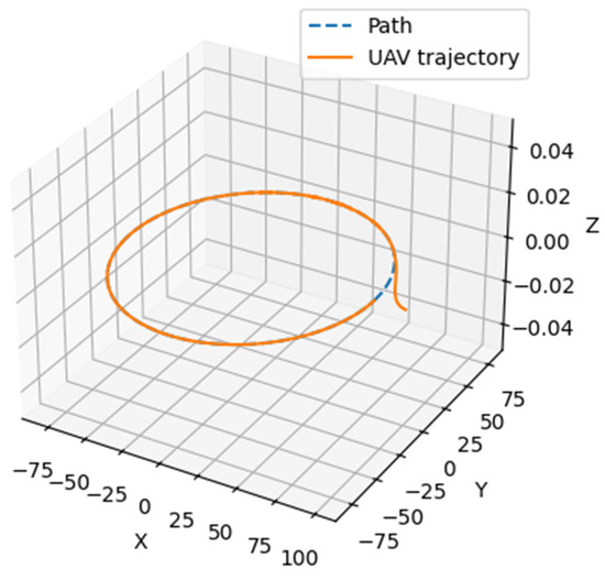
Figure 9.
Visual representation of the implementation of Scenario 4 (circular trajectory with variable speed).
The analysis of the UAV’s behavior in this scenario made it possible to demonstrate the initial adaptation phase, which lasts approximately 10 s. During this stage, a significant deviation of the actual trajectory from the ideal one is observed, indicating the need to correct the initial heading. As in previous cases, this is caused by the inertial properties of the UAV and the delay in speed stabilization.
The next phase is the correction phase, lasting approximately 10–30 s. During this period, the UAV gradually reduces its deviation and adjusts its position in accordance with the assigned trajectory. This indicates the operability of the control regulator, which adapts to changes in speed.
In the subsequent stabilization phase (beyond 30 s), the UAV almost completely aligns with the desired trajectory, demonstrating stable control. Minor oscillations may be caused by the characteristics of the regulator or the influence of external disturbances.
The variable speed profile—with initial acceleration (up to 15 s) and subsequent deceleration (15–25 s)—caused nonlinear deviations, especially during the transient processes. This is clearly visible in Figure 10, which presents a graph of UAV deviation changes along the X and Y axes over time when following a circular trajectory with variable speed. The results of this graph effectively confirm the need for adaptive control to minimize dynamic errors.
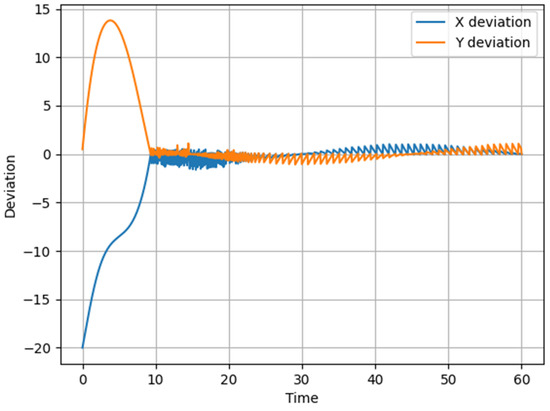
Figure 10.
Graph of UAV deviation in X and Y coordinates relative to the specified circular trajectory over time during the implementation of Scenario 3.
A noticeable initial deviation spike is observed during the first 10 s. The X-axis (blue line) shows a descending nonlinearity reaching a maximum deviation of approximately –20 m. The Y-axis (orange line) initially shows a significant positive peak (≈15 m), indicating a sharp corrective maneuver.
Both deviations gradually decrease in the time range from 10 to 30 s, confirming the functionality of the corrective control.
Thereafter, oscillations are damped, and the values converge toward zero. After the 30s mark, deviations stabilize within ±1 m, indicating convergence to a steady-state.
Minor oscillations may be caused by algorithmic characteristics of the control or sensor accuracy.
Significant initial deviations indicate the system’s high sensitivity to speed changes. The proposed algorithm effectively compensates for trajectory errors, demonstrating a gradual reduction in deviation. This confirms that the use of variable speed requires more flexible adaptive control to ensure smooth trajectory tracking.
2.2.4. Consideration of UAV Aerodynamic Characteristics
The aerodynamic characteristics of an unmanned aerial vehicle (UAV) play a key role in shaping its flight trajectory, maneuverability, and stability. Considering these characteristics is necessary for the accurate modeling of flight dynamics, effective trajectory control, and maintaining UAV stability under various operational conditions.
To improve the accuracy of trajectory calculation and flight control, it is necessary to consider the following key aerodynamic characteristics.
Aerodynamic drag (D): the force acting opposite to the UAV’s direction of motion due to air friction and frontal resistance. Affects energy consumption and maximum speed.
Lift (L): generated by wings or rotors, enabling the UAV to stay airborne. Determines the ability to maintain flight altitude.
Lift (CL) and drag (CD) coefficients: define the aerodynamic efficiency of the wing and influence energy consumption during maneuvers.
Aerodynamic efficiency (L/D): characterizes flight performance; higher values indicate that the UAV can travel longer distances with minimal energy expenditure.
Stability and controllability: depend on the position of the center of mass, surface area of control surfaces, and aerodynamic moments affecting motion.
Realistic UAV trajectory modeling requires accounting for aerodynamic influences during changes in speed, direction, and maneuver execution. The main influencing factors are as follows. At low speeds, lift and drag dominate, requiring an increased angle of attack or engine power. At high speeds, air resistance increases, limiting maneuvering capabilities and requiring optimized wing profiles. During turns, the UAV must balance lift and centrifugal forces, affecting trajectory stability. For variable-speed flight, it is crucial to control the balance between thrust and aerodynamic drag to avoid excessive energy consumption or flow separation.
In trajectory modeling in a single plane with aerodynamic considerations, it is necessary to retain the effects of aerodynamic drag and wind. At the same time, lift can be temporarily ignored, as, under simplified scenarios, it does not affect modeling quality significantly.
To account for aerodynamic effects correctly in UAV motion modeling, nonlinear aerodynamic effects were included in the mathematical model. In addition, the model provides for the use of variable thrust and angle-of-attack control to optimize flight across various speeds. Model adaptation to real-world conditions through flight data analysis and parameter correction was used to account for external influences.
In the modeling, the aerodynamic drag coefficient was assumed as Cd = 0.05. For the case of constant UAV speed, V = 5 m/s was used. Lateral wind speed Vwind was modeled as a periodic function: Vwind = 0.2 sin(2πt/T).
The proposed model is most suitable for small and medium fixed-wing UAVs such as Boeing Insitu ScanEagle, AeroVironment Puma 3 AE, and UAV Factory Penguin C.
The simulation results considering UAV aerodynamic characteristics are shown in Figure 11 and Figure 12. These figures provide a visual representation of the implementation of previously used scenarios and also show graphs of UAV deviations in X and Y coordinates relative to the assigned trajectories over time for those scenarios.
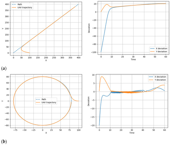
Figure 11.
Visual representation of the implementation of scenarios with constant speed and graphs of the UAV deviation in X and Y coordinates relative to the set trajectory over time during the implementation of scenarios (straight (a) and circular (b) trajectories).
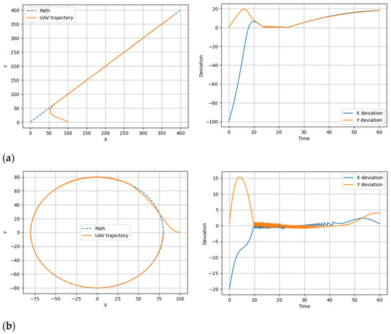
Figure 12.
Visual representation of the implementation of scenarios with variable speed and graphs of the UAV deviation in the X and Y coordinates relative to the set trajectory over time during the implementation of scenarios (straight (a) and circular (b) trajectories).
Thus, according to the results of the simulation, it can be noted that aerodynamic drag significantly affects control, especially at high speeds. It is also evident from Figure 12 and Figure 13 that variable speed complicates stabilization, which requires the adaptive tuning of the control coefficients. In addition, the research results showed that lateral wind causes periodic deviations, which can be compensated by correction algorithms.
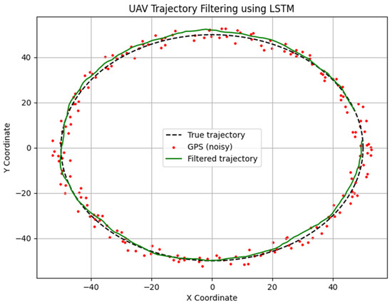
Figure 13.
Simulation Results and UAV Trajectory Filtering Using an LSTM Neural Network.
It should be noted that despite the positive results in the previous stage of UAV trajectory tracking simulation, we considered aerodynamic characteristics without real sensor errors.
In reality, however, the UAV receives information from sensors that are subject to noise, delays, and inaccuracies. These factors can significantly degrade navigation accuracy and lead to deviations from the intended trajectory.
Therefore, the next step of the research is to collect real or simulated sensor data and filter this data using RNNs.
2.3. Sensor Data Collection and Filtering Using RNN
An analysis of UAV navigation system structures has shown that they consist of several key sensors. Sensors provide information about the UAV’s position, speed, acceleration, and other motion parameters. The main navigation sensors include:
- −
- GPS—used for determining the global position of the UAV, but it has an error of 2–5 m depending on signal conditions;
- −
- IMU (Inertial Measurement Unit)—contains accelerometers and gyroscopes that measure acceleration and angular velocity, but the main issue is drift accumulation (0.1–1° per minute);
- −
- barometric altimeter—determines altitude based on air pressure, but the error can range from 3–10 m due to weather changes;
- −
- lidar or visual sensors—used for local navigation, but their data can be noisy due to lighting or weather conditions.
Based on this, the problems arising in navigation data are associated with several risks. First is noise—random signal fluctuations that make it difficult to determine coordinates accurately. Second is IMU drift—the gradual accumulation of error that leads to position offset. Third is data lag–measurement delay that causes instability in control. If these errors are not compensated for, the control system will respond to incorrect coordinates, leading to even greater deviations from the trajectory.
Studies have shown that filtering methods are used to reduce noise and improve trajectory accuracy. Traditional methods include:
- −
- Kalman Filter (KF)—works well in linear systems but has limitations in complex nonlinear dynamic models;
- −
- Complementary Filter—effective for combining GPS and IMU, but it does not compensate for delay and drift;
- −
- Recurrent Neural Networks (RNNs)—have the ability to analyze time series and adapt to changes in navigation data.
It should be noted that this is not an exhaustive list of possible solutions. However, analysis and conducted research have led to the conclusion that these methods, especially RNN-based solutions, are promising. In this study, it was decided to focus on RNNs, which use feedback between time steps. This allows not only for noise smoothing but also for predicting future positions. This is particularly important for UAVs, as even small delays can cause flight instability.
The developed RNN model operates as follows. The input to the network is a sequence of values from GPS, IMU, wind speed, and accelerometers. The RNN (LSTM/GRU) processes the historical data and predicts corrected coordinates. The output consists of the filtered position, velocity, and acceleration values of the UAV.
Formally, the RNN model receives a sequence of input measurements X = (x1,x2,…,xt) and outputs the corrected coordinates Y = (y1,y2,…,yt).
where W, U, b are network parameters and ht−1 is the previous time step’s state.
For training the LSTM filtering model, we used a simulated dataset that includes UAV trajectories affected by GPS noise, IMU drift, and sensor latency. Ground truth positions were generated from the clean simulated trajectory data before noise was injected. To ensure generalization and reduce the risk of overfitting, the training set included multiple trajectory types (linear, circular, spiral) and different environmental conditions (wind variations, sensor dropout intervals). A validation set was held out for early stopping, and the final loss curve (Table 1) indicates convergence without signs of overfitting. While the model has only been trained on simulated data, its robustness is supported by diverse training samples and will be further evaluated under real-world conditions in future work.

Table 1.
RNN Filter Training Dynamics for UAV Sensor Data Error Compensation.
3. Results
To evaluate the effectiveness of applying a Recurrent Neural Network (RNN) for sensor data filtering, a series of experimental studies was conducted using simulated measurements. The purpose of the simulation was to assess the level of data smoothing and error compensation that occurs during the determination of the UAV’s position and orientation.
Several assumptions were made during the study. First, the simulation took into account the main characteristics of sensor errors typical of modern UAV navigation systems, namely:
GPS error, or GPS measurement coordinates containing random deviations due to satellite positioning errors:
where U(−3,3) is a uniform distribution of errors within ±3 m; xgps, ygps—measured coordinates; xtrue, ytrue—true coordinates, ξgps, ηgps—random GPS errors.
xgps = xtrue + ξgps, ξgps∼U(−3,3);
ygps = ytrue + ηgps, ηgps∼U(−3,3),
This represents random coordinate displacement within ±3 m, simulating typical inaccuracies of satellite positioning due to multipath effects and signal delays.
IMU drift, or the gradual shift of the angle by 1° over 60 s, resulting from the integration of noisy signals from accelerometers and gyroscopes:
where is the current angle value; is the previous angle value.
Signal delay τ∼U(0.1,0.3)—a random measurement lag within 0.1–0.3 s, representing possible delays in data transmission between the sensors and the computational module.
During testing, the RNN system received input data from the GPS and IMU and simulated the predicted UAV position at future time steps, smoothing errors and correcting the received values.
As seen in Figure 13, the visualization of the simulation results includes three key components: the true trajectory, the GPS measurements, and the filtered trajectory.
The true trajectory shows the theoretically correct path the UAV was supposed to follow. The GPS measurement points show noisy data obtained from the Global Positioning System (GPS), clearly displaying significant deviations due to satellite signal errors. The filtered trajectory is the result of processing the noisy GPS data using an LSTM neural network.
From Figure 13, it can be seen that deviations after applying the LSTM decreased by approximately 3 to 5 times compared to the original GPS data. This highlights the effectiveness of the studied model.
The results in Table 1 demonstrate the training dynamics of the RNN model used for filtering sensor data and compensating for GPS and IMU errors.
The table shows the breakdown of results into several phases:
Initial training phase (Epochs 1–5). In the first epoch, the loss function value is 0.2443, which is relatively high. However, by the second epoch, the loss significantly decreases to 0.0324, indicating a rapid adjustment of the model. By the fifth epoch, the error drops to 0.0015, demonstrating effective training and model adaptation to sensor data.
Training stabilization phase (Epochs 6–20). Starting from the sixth epoch, the loss gradually decreases to a level of 7.5348 × 10⁻⁴ (≈0.00075). It can be observed that by epoch 10, the loss stabilizes within the range of 3.8 × 10⁻⁴ to 4.0 × 10⁻⁴. Furthermore, between epochs 15 and 20, the model reaches a minimum loss value of 3.07 × 10⁻⁴, after which only minor fluctuations are observed.
Overfitting or optimization oscillation phase (Epochs 21–25…). Between epochs 21 and 25, the loss remains within the range of 3.0 × 10⁻⁴ to 4.0 × 10⁻⁴, sometimes exhibiting slight oscillations, which indicates the sufficient generalization capability of the model.
To address the robustness of the RNN and RL modules, we conducted a sensitivity analysis of the key hyperparameters, including the learning rate, number of hidden units, and discount factor. The parameter selection process was performed through empirical tuning using a validation set consisting of multiple simulated trajectories with varying levels of sensor noise and environmental disturbances.
For the RNN module, we compared configurations with hidden layer sizes ranging from 32 to 128 units and observed that models with fewer than 64 units underfit the data while those with more than 128 units tended to overfit. A hidden layer size of 96 units with a learning rate of 0.001 provided the best trade-off between generalization and convergence speed.
For the RL module (based on PPO), sensitivity tests with varying discount factors (γ ∈ [0.85, 0.99]) showed that values below 0.9 led to unstable behavior while γ = 0.95 provided consistent results in obstacle avoidance and trajectory adherence.
These results confirm that the system maintains stable performance under a range of parameter configurations and is not overly sensitive to specific hyperparameter values.
Thus, a method has been implemented for collecting real or simulated sensor data and filtering it using an RNN.
The analysis of the obtained data allows us to draw the following conclusions regarding the effectiveness of the proposed approach:
The graphs of the raw sensor data show significant fluctuations, which complicate the determination of the actual trajectory. However, after RNN processing, the UAV’s trajectory becomes smoother, and GPS errors are significantly reduced, indicating effective filtering. IMU errors, particularly accumulated drift, are almost completely compensated, as the network takes previous states into account and effectively suppresses the gradual accumulation of error. UAV trajectory deviations from the target path after RNN filtering are reduced by 2–3 times, which significantly improves the accuracy of autonomous navigation.
Overall, the simulation results confirm the feasibility of using recurrent neural networks to enhance UAV navigation accuracy by smoothing sensor errors and compensating for drift.
To provide a quantitative benchmark, we implemented two baseline navigation strategies under identical simulated conditions:
- −
- a Kalman filter for GPS/IMU fusion combined with a PID controller for trajectory correction, and
- −
- a classical Model Predictive Controller (MPC) for trajectory tracking.
All methods were evaluated under conditions of sensor noise, IMU drift, and intermittent GPS loss.
Table 2 summarizes the average trajectory deviation and response time.
Table 2.
Comparative performance under sensor degrada.
The results demonstrate that the proposed approach achieves up to 60% lower average deviation and significantly faster recovery compared to standard navigation methods. This confirms the advantage of integrating data-driven filtering and learning-based control under degraded sensing conditions.
To evaluate the computational feasibility of the proposed approach, we analyze the performance overhead introduced by the RNN-based sensor filtering and reinforcement learning modules. The LSTM filter processes sequential sensor data (e.g., GPS, IMU, wind) with input dimension nnn and hidden size h, resulting in time complexity O(T*h2) per sequence of length T. In our implementation, input dimensionality is low (n ≤ 8) and hidden state size moderate (h = 32), allowing for real-time inference on embedded hardware.
The reinforcement learning module, trained offline, performs trajectory adjustment using a shallow neural network. Its online inference requires only a single forward pass, yielding constant-time complexity O(n) during deployment. Both modules maintain sub-50 ms latency on standard UAV processors (e.g., Raspberry Pi 4 or Jetson Nano). Thus, the architecture achieves a favorable balance between computational demand and autonomy, supporting real-time onboard operation.
4. Discussion
This study proposed a comprehensive approach to ensuring the resilient navigation of an unmanned aerial vehicle (UAV) under conditions of limited or unstable sensor information. The simulation results demonstrate the effectiveness of the proposed architecture, which combines geometric trajectory representation, the filtering of noisy data using recurrent neural networks, and adaptive control based on reinforcement learning methods.
The LSTM-based filtering module provided a smoothing of unstable GPS and IMU data, reducing positioning errors and allowing the model to operate even under conditions of partial signal loss. This enables the system to be applied in real-world scenarios where access to precise positioning or imaging is limited—such as in urban canyons, dense forests, or disaster zones. The geometric trajectory modeling based on path coordinates ensured stability and predictability of movement, which is especially important for executing precise maneuvers and safely avoiding obstacles [27].
The proposed reinforcement learning module allowed the system to adaptively respond to dynamic environmental changes, particularly to detect and avoid obstacles without the need for a pre-mapped environment [28,29]. This makes the method suitable for use in uncertain environments where unpredictable risks or changes may occur.
Another important component is the adaptive speed regulation block, which allows for motion optimization depending on mission priorities, environmental risks, or constraints. This contributes to increased energy efficiency, reduced unnecessary maneuvers, and extended autonomous flight time, which is extremely important in the context of sustainable development.
Compared to classical navigation methods that rely on stable signals or a complete set of sensors, the proposed system demonstrates enhanced resilience and flexibility. It can be effectively applied across various fields—from humanitarian logistics and environmental monitoring to emergency response and agricultural control.
Furthermore, to support the practical value of our approach, we conducted a benchmarking analysis comparing the proposed LSTM and RL-based architecture with traditional methods, including the Kalman filter and PID controllers, under conditions of sensor degradation. These experiments, described in Section 3, show that our method achieves significantly lower trajectory deviation (up to 3× improvement), maintains stable real-time performance (<50 ms inference latency), and remains robust under sensor dropouts, outperforming the classical baselines in both accuracy and adaptability. This quantitative validation reinforces the applicability of the system in real-world conditions where conventional approaches may fail.
However, it is important to note that the simulation environment, while incorporating aerodynamic drag and wind disturbances, does not fully account for other real-world factors such as GPS multipath effects in urban environments, sensor data dropouts, thermal drift of IMUs, and computation limitations of embedded hardware. These factors may significantly affect navigation reliability and system responsiveness during real missions. In future work, we aim to address these gaps through hardware-in-the-loop (HIL) testing [30,31], field trials in degraded GNSS conditions, and performance benchmarking on resource-constrained platforms. This will enable more comprehensive evaluation and improve confidence in practical deployment.
While the simulation environment incorporated aerodynamic drag and wind disturbances, it did not fully account for key real-world factors such as GPS multipath effects, sensor data dropouts, IMU drift, and the computational limitations of embedded onboard hardware. These limitations may significantly affect navigation reliability and responsiveness. To address this, future work will include HIL testing, real-world UAV flight experiments in degraded GNSS environments, and performance benchmarking under onboard processing constraints. Such efforts are essential to validate the proposed method under operational conditions and improve confidence in its practical deployment. Future research will involve HIL testing and real-world flight experiments to validate the robustness of the approach under these conditions. Such validation will focus on assessing the impact of GPS multipath effects, latency in sensor fusion, computational performance on onboard processors, and the real-time responsiveness of the RL-based controller. These efforts are critical to increase confidence in the method’s deployment in practical missions and to ensure safety, reliability, and adaptability in real-world UAV applications.
Moreover, we acknowledge that the current model does not explicitly address certain safety-critical aspects such as sensor spoofing, cybersecurity vulnerabilities, or fail-safe fallback mechanisms in case of sensor loss or control failures. These limitations are particularly relevant for UAV applications in degraded or contested environments. As part of future work, we plan to explore the integration of anomaly detection in sensor streams, lightweight redundancy for fallback control, and basic cyber-resilience techniques into the navigation stack. These additions are essential to support safe operation in unpredictable real-world scenarios and to extend the robustness of the proposed architecture.
Thus, the developed approach lays the foundation for the creation of autonomous intelligent navigation systems capable of ensuring safe, energy-efficient, and reliable UAV operation even in complex and unstable environments—an essential factor for the sustainable development of future infrastructure.
While this work discusses the relevance of the proposed navigation architecture to the Sustainable Development Goals (SDG 9, 11, 13), we acknowledge that such alignment must be substantiated with quantitative criteria. However, several results obtained in our study demonstrate clear technical improvements that serve as enablers for sustainable UAV deployment in real-world environments.
First, the use of an LSTM-based sensor filtering module significantly reduces the positioning noise and compensates for IMU drift, leading to a 2–3× decrease in trajectory deviation. This directly enhances navigation resilience, which is a critical component of SDG 9 (resilient infrastructure) and SDG 11 (urban safety). The ability of UAVs to maintain stable trajectories even in the presence of degraded or delayed sensor data enables safer operations in urban canyons, disaster zones, or areas with weak GNSS signals.
Second, the adaptive reinforcement learning-based control policy enables real-time response to environmental uncertainties without the need for a full sensor suite or pre-mapped environments. This reduces the dependency on ground infrastructure and allows for the flexible deployment of UAVs in emerging regions or in post-disaster scenarios—both of which are emphasized in SDG 11 and SDG 13.
Third, the adaptive speed regulation module contributes to energy efficiency by reducing unnecessary maneuvers and flight oscillations. Simulation results indicate smoother path following and lower control effort, which translates to longer flight endurance on a fixed energy budget. While we do not directly model lifecycle carbon emissions or battery drain, the improvements in control smoothness and trajectory stability form an important technical basis for subsequent sustainability assessment.
In future work, we intend to complement these engineering improvements with quantitative sustainability metrics—such as mission energy usage, risk-aware deployment models, and measurable SDG indicators—to better capture the real-world environmental and societal impact of UAV navigation systems.
5. Conclusions
The article presents the development of an intelligent autonomous UAV motion control method under conditions of visual data deficiency. The proposed approach is based on the use of adaptive machine learning algorithms for trajectory correction, which ensures flight stability even in the absence of complete environmental information. The main feature of the developed method is the synthesis of control based on path coordinates and normal form theory, enabling the effective reduction of deviations from the assigned route and real-time obstacle avoidance.
The scientific novelty of the work lies in the integrated use of machine learning algorithms with path coordinate methods for sensor data filtering and UAV trajectory stabilization under visual information scarcity. A distinctive aspect of the proposed approach compared to existing solutions is the enhancement of recurrent neural network (RNN) methods through architecture optimization and model training to compensate for sensor errors, which improves navigation accuracy and minimizes positioning errors.
The practical significance of the method is determined by its capability to provide UAV control in limited visibility conditions. The use of RNNs for sensor data filtering made it possible to reduce GPS navigation errors by 2.5–3 times and IMU errors by 2 times, ensuring more accurate positioning and stable UAV movement in dynamic environments.
The obtained results can be applied to perform various missions, including monitoring, rescue operations, cargo delivery, and reconnaissance. The implementation of the method improves route tracking accuracy, minimizes energy consumption for flight correction, and optimizes the motion trajectory, contributing to increased UAV flight autonomy.
Thus, the developed method enables autonomous UAV control under visual data deficiency, allows for adaptive obstacle avoidance, and significantly enhances navigation accuracy. It lays the foundation for the further development of intelligent navigation systems that can be integrated into various fields, including military, rescue, and logistics operations.
Author Contributions
Conceptualization, S.S.; methodology, S.S. and O.W.; software, P.M. and J.Y.; validation, M.K.-K., O.W. and J.Y.; formal analysis, S.S., L.G. and O.C.; investigation, M.K.-K., L.G. and J.H.; data curation, P.M., B.K. and J.H.; writing—original draft preparation, S.S.; writing—review and editing, S.S.; visualization, M.K.-K., B.K. and O.C.; supervision, S.S. All authors have read and agreed to the published version of the manuscript.
Funding
This research received no external funding.
Institutional Review Board Statement
Not applicable.
Informed Consent Statement
Not applicable.
Data Availability Statement
The raw data supporting the conclusions of this article will be made available by the authors on request.
Conflicts of Interest
The authors declare no conflicts of interest. Author Jian Yu was employed by the company Zhongke Shuguang. Author Jiang He was employed by the company CNOOC Financial Shared Service Center PRD Branch. The remaining authors declare that the research was conducted in the absence of any commercial or financial relationships that could be construed as a potential conflict of interest.
References
- Radzki, G.; Nielsen, I.; Golińska-Dawson, P.; Bocewicz, G.; Banaszak, Z. Reactive UAV Fleet’s Mission Planning in Highly Dynamic and Unpredictable Environments. Sustainability 2021, 13, 5228. [Google Scholar] [CrossRef]
- AL-Dosari, K.; Fetais, N. A New Shift in Implementing Unmanned Aerial Vehicles (UAVs) in the Safety and Security of Smart Cities: A Systematic Literature Review. Safety 2023, 9, 64. [Google Scholar] [CrossRef]
- Adel, G.; Anuar, A.; Ruzairi, R.; Supa’at, A.S.M.; Shukor, R.; Mohammed, G. Involvement of Surveillance Drones in Smart Cities: A Systematic Review. IEEE Access 2022, 10, 56611–56628. [Google Scholar] [CrossRef]
- Sousa, M.; Almeida, M.F.; Calili, R. Multiple Criteria Decision Making for the Achievement of the UN Sustainable Development Goals: A Systematic Literature Review and a Research Agenda. Sustainability 2021, 13, 4129. [Google Scholar] [CrossRef]
- Semenov, S.; Krupska-Klimczak, M.; Mazurek, P.; Zhang, M.; Chernikh, O. Improving Unmanned Aerial Vehicle Security as a Factor in Sustainable Development of Smart City Infrastructure: Automatic Dependent Surveillance–Broadcast (ADS-B) Data Protection. Sustainability 2025, 17, 1553. [Google Scholar] [CrossRef]
- Semenov, S.; Kolisnyk, T.; Oksana, S.; Roh, V. Intelligent extraction of the informative features for UAV motion modelling: Principles and techniques. In Proceedings of the 2023 13th International Conference on Dependable Systems, Services and Technologies (DESSERT), Athens, Greece, 13–15 October 2023; pp. 1–6. [Google Scholar] [CrossRef]
- Agrawal, S.; Patle, B.K.; Sanap, S. Navigation control of unmanned aerial vehicles in dynamic collaborative indoor environment using probability fuzzy logic approach. Cogn. Robot. 2025, 5, 86–113. [Google Scholar] [CrossRef]
- Wu, P.; Clothier, R.; Campbell, D.; Walker, R. Fuzzy Multi-Objective Mission Flight Planning in Unmanned Aerial Systems. In Proceedings of the 2007 IEEE Symposium on Computational Intelligence in Multi-Criteria Decision-Making, Honolulu, HI, USA, 1–5 April 2007; pp. 2–9. [Google Scholar] [CrossRef]
- Jiang, C.; Chen, S.; Chen, Y.; Zhang, B.; Feng, Z.; Zhou, H.; Bo, Y. A MEMS IMU De-Noising Method Using Long Short Term Memory Recurrent Neural Networks (LSTM-RNN). Sensors 2018, 18, 3470. [Google Scholar] [CrossRef]
- Mao, N.; Xu, J.; Li, J.; He, H. A LSTM-RNN-Based Fiber Optic Gyroscope Drift Compensation. Math. Probl. Eng. 2021, 2021, 1636001. [Google Scholar] [CrossRef]
- Hernandez-Ossa, K.A.; Montenegro-Couto, E.H.; Longo, B.; Bissoli, A.; Sime, M.M.; Lessa, H.M.; Enriquez, I.R.; Frizera-Neto, A.; Bastos-Filho, T. Simulation System of Electric-Powered Wheelchairs for Training Purposes. Sensors 2020, 20, 3565. [Google Scholar] [CrossRef]
- Forkan, M.; Rizvi, M.M.; Chowdhury, M.A.M. Optimal path planning of Unmanned Aerial Vehicles (UAVs) for targets touring: Geometric and arc parameterization approaches. PLoS ONE 2022, 17, e0276105. [Google Scholar] [CrossRef]
- Zhang, B.; Mao, Z.; Liu, W.; Liu, J. Geometric Reinforcement Learning for Path Planning of UAVs. J. Intell. Robot. Syst. 2015, 77, 391–409. [Google Scholar] [CrossRef]
- Semenov, S.; Jian, Y.; Jiang, H.; Chernykh, O.; Binkovska, A. MATHEMATICAL MODEL OF INTELLIGENT UAV FLIGHT PATH PLANNING. Adv. Inf. Syst. 2025, 9, 49–61. [Google Scholar] [CrossRef]
- Solaimalai, G.; Prakash, K.J.; Sampath Kumar, S.; Bhagyalakshmi, A.; Siddharthan, P.; Kumar, K.R.S. Deep Reinforcement Learning for Autonomous Drone Navigation in Cluttered Environments. In Proceedings of the 2024 International Conference on Advances in Computing, Communication and Applied Informatics (ACCAI), Chennai, India, 25 July 2024; pp. 1–5. [Google Scholar] [CrossRef]
- Julian, K.D.; Kochenderfer, M.J. Guaranteeing Safety for Neural Network-Based Aircraft Collision Avoidance Systems. In Proceedings of the 2019 IEEE/AIAA 38th Digital Avionics Systems Conference (DASC), San Diego, CA, USA, 8–12 September 2019; pp. 1–10. [Google Scholar] [CrossRef]
- Joglekar, A.; Krovi, V.; Brudnak, M.; Smereka, J.M. Hybrid Reinforcement Learning based controller for autonomous navigation. In Proceedings of the 2022 IEEE 95th Vehicular Technology Conference: (VTC2022-Spring), Helsinki, Finland, 19–22 June 2022; pp. 1–6. [Google Scholar] [CrossRef]
- Ahmed, G.; Sheltami, T. Novel Energy-Aware 3D UAV Path Planning and Collision Avoidance Using Receding Horizon and Optimization-Based Control. Drones 2024, 8, 682. [Google Scholar] [CrossRef]
- Erdal, K.; Ahmadieh, K.M.; Jaime, R.-H.; Reyhanoglu, M. Learning Control of Fixed-Wing Unmanned Aerial Vehicles Using Fuzzy Neural Networks. Int. J. Aerosp. Eng. 2017, 2017, 5402809. [Google Scholar] [CrossRef]
- Tuśnio, N.; Wróblewski, W. The Efficiency of Drones Usage for Safety and Rescue Operations in an Open Area: A Case from Poland. Sustainability 2022, 14, 327. [Google Scholar] [CrossRef]
- Miljana, S.; Maj, S.; Gjorgji, N.; Marko, B.; Matjaz, G. Artificial Intelligence-Based Decision Support System for Sustainable Urban Mobility. Electronics 2024, 13, 3655. [Google Scholar] [CrossRef]
- Angel, R.; Paul, B.; Yvonne, S.; Roy, S.; John, L. Nonlinear Control of Quadcopters via Approximate Dynamic Programming. In Proceedings of the 2019 18th European Control Conference (ECC), Naples, Italy, 25–28 June 2019; pp. 3752–3759. [Google Scholar] [CrossRef]
- Siwek, M.; Panasiuk, J.; Baranowski, L.; Kaczmarek, W.; Borys, S. Trajectory Tracking Control of a Mobile Robot with the ROS System. Probl. Mechatron. Armament Aviat. Saf. Eng. 2022, 13, 67–84. [Google Scholar] [CrossRef]
- Wang, X.; Ye, X.; Zhou, Y.; Li, C. Path-Following Control of Unmanned Vehicles Based on Optimal Preview Time Model Predictive Control. World Electr. Veh. J. 2024, 15, 221. [Google Scholar] [CrossRef]
- Li, J.; Lou, J.; Li, Y.; Pan, S.; Xu, Y. Trajectory Tracking of Autonomous Vehicle Using Clothoid Curve. Appl. Sci. 2023, 13, 2733. [Google Scholar] [CrossRef]
- Park, S. Three-Dimensional Dubins-Path-Guided Continuous Curvature Path Smoothing. Appl. Sci. 2022, 12, 11336. [Google Scholar] [CrossRef]
- Guang, X.; Gao, Y.; Liu, P.; Li, G. IMU Data and GPS Position Information Direct Fusion Based on LSTM. Sensors 2021, 21, 2500. [Google Scholar] [CrossRef] [PubMed]
- Tang, P.; Li, J.; Sun, H. A Review of Electric UAV Visual Detection and Navigation Technologies for Emergency Rescue Missions. Sustainability 2024, 16, 2105. [Google Scholar] [CrossRef]
- Semenov, S.; Voloshyn, D.; Lymarenko, V.; Semenova, A.; Davydov, V. Method of UAVs Quasi-Autonomous Positioning in the External Cyber Attacks Conditions. In Proceedings of the 2019 10th International Conference on Dependable Systems, Services and Technologies (DESSERT), Leeds, UK, 5–7 June 2019; pp. 149–153. [Google Scholar] [CrossRef]
- Kotsampopoulos, P.; Lagos, D.; Hatziargyriou, N.; Omar Faruque, M.; Lauss, G.; Nzimako, O.; Forsyth, P.; Steurer, M.; Ponci, F.; Monti, A.; et al. A Benchmark System for Hardware-in-the-Loop Testing of Distributed Energy Resources. IEEE Power Energy Technol. Syst. J. 2018, 5, 94–103. [Google Scholar] [CrossRef]
- Gao, Y.; Xu, Z.; Zhao, X.; Wang, G.; Yuan, Q. Hardware-in-the-Loop Simulation Platform for Autonomous Vehicle AEB Prototyping and Validation. In Proceedings of the 2020 IEEE 23rd International Conference on Intelligent Transportation Systems (ITSC), Rhodes, Greece, 20–23 September 2020; IEEE Press: Piscataway, NJ, USA, 2020; pp. 1–6. [Google Scholar] [CrossRef]
Disclaimer/Publisher’s Note: The statements, opinions and data contained in all publications are solely those of the individual author(s) and contributor(s) and not of MDPI and/or the editor(s). MDPI and/or the editor(s) disclaim responsibility for any injury to people or property resulting from any ideas, methods, instructions or products referred to in the content. |
© 2025 by the authors. Licensee MDPI, Basel, Switzerland. This article is an open access article distributed under the terms and conditions of the Creative Commons Attribution (CC BY) license (https://creativecommons.org/licenses/by/4.0/).