
Optimal Distributed Generation Mix to Enhance Distribution Network Performance: A Deterministic Approach

 , ,
, ,
Abstract
1. Background
- i.
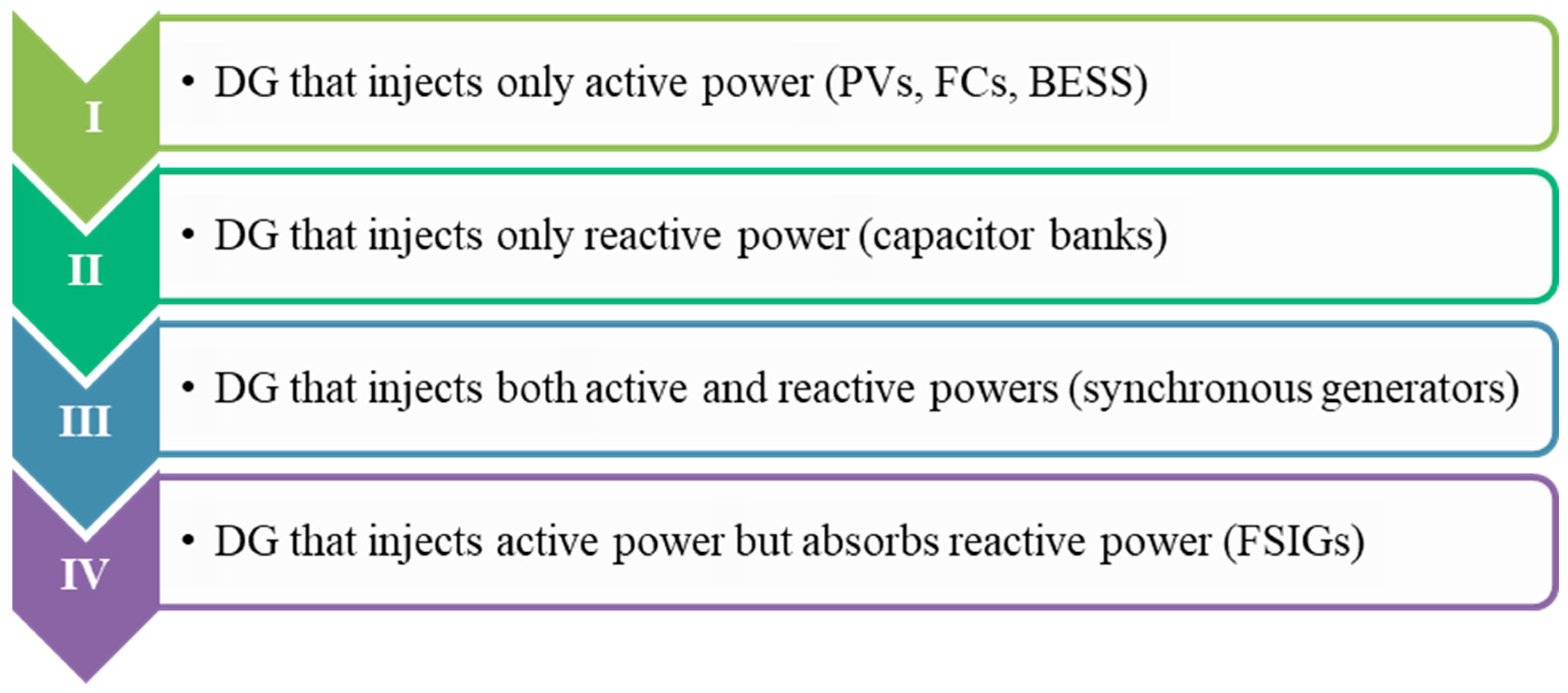
- A new, realistic DG type with active power injecting and dynamically adjusting (absorbing or injecting) reactive power capabilities has been introduced.
- ii.
- The existing four DG types in the literature have been limited to three proposed types, i.e., type-II DG injecting reactive power, type-III DG injecting both active and reactive powers, and type-IV DGs injecting active power and dynamically adjusting (absorbing or injecting) reactive power.
- iii.
- The optimal combination of the proposed three DG types has been determined using the algorithm-specific parameter-free Jaya optimization (JO) technique. Although JO is already a well-established technique, its exclusive application to the proposed optimization problem to attain the optimal mix of the proposed three DG types has been explored.
- iv.
- The effectiveness of the proposed approach of simultaneously allocating the suggested three DG types against the existing DG types available in the literature has been examined.
2. Significance of the Research
- i.
- Regulate the voltage of weak, distant buses.
- ii.
- Prevent against the over- and under-voltages.
- iii.
- Reduce power losses, both active and reactive, by supplying power close to the load centers.
- iv.
- Act as a backup source in case of grid failure. Thus, it allows the distribution networks to operate in islanded mode, such as in rooftop solar photovoltaic systems.
- v.
- Enhance the reliability of power systems by acting as a backup source.
- vi.
- Allow consumers to use net metering, thus lowering their electricity bills.
- vii.
- Lower utilities’ operational costs, thus enhancing their revenue.
- viii.
- Defer or avoid the upgradation of power system infrastructure.
- ix.
- Renewable-based DGs (RE-DGs), like solar, wind, etc., can reduce greenhouse gas (GHG) emissions and carbon footprints.
- x.
- Reduce fossil-fuel dependence by enhancing the RE-DG penetration in the electric grid.
3. Problem Formulation
3.1. Fitness Function
3.2. Constraints
4. Jaya Optimization Algorithm
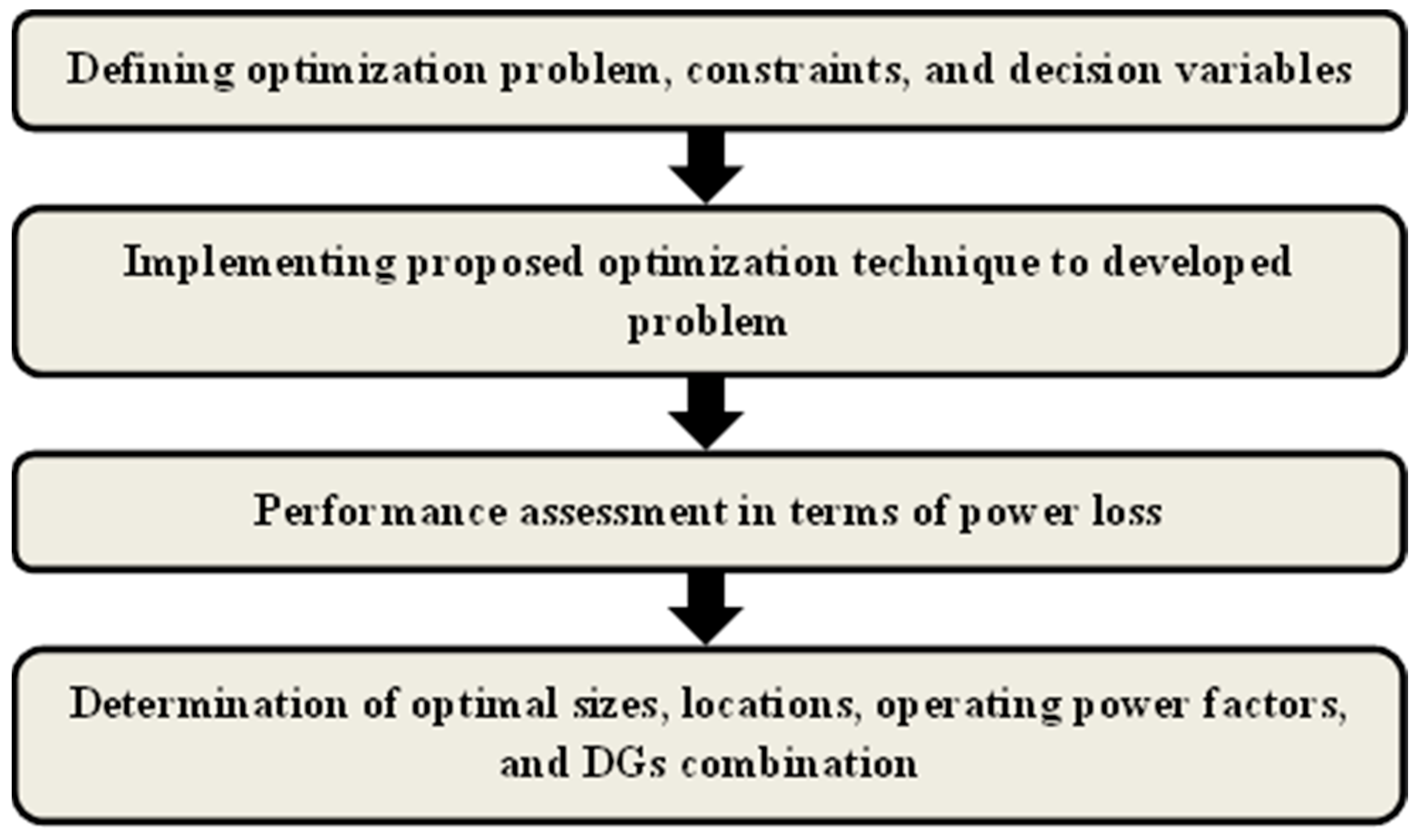
Implementing JO in Proposed Problem
- i.
- Setting the JO parameters, such as agent population and iteration count, is the starting step of the proposed optimization problem.
- ii.
- Initializing candidate solutions is the second step.
- iii.
- Initializing the iteration count is the third step.
- iv.
- The fourth phase analyzes the load flow to compute the initial values of the fitness function.
- v.
- The fifth step checks the iteration count.
- vi.
- The sixth step is to update the solutions using JO’s updating equation.
- vii.
- The seventh phase re-performs the load flow to compute each iteration’s candidate solutions’ fitness values.
- viii.
- The eighth step loops or ends the iterations for solution updating, after which the algorithm stops.
5. Results and Discussion
5.1. Results for Type-II DG (Supply Active Power)
| DG Type | PDG Active power output | QDG Reactive power output | |
| Type-II | PDG = 0 | QDG = SDG | (10) |
- i.
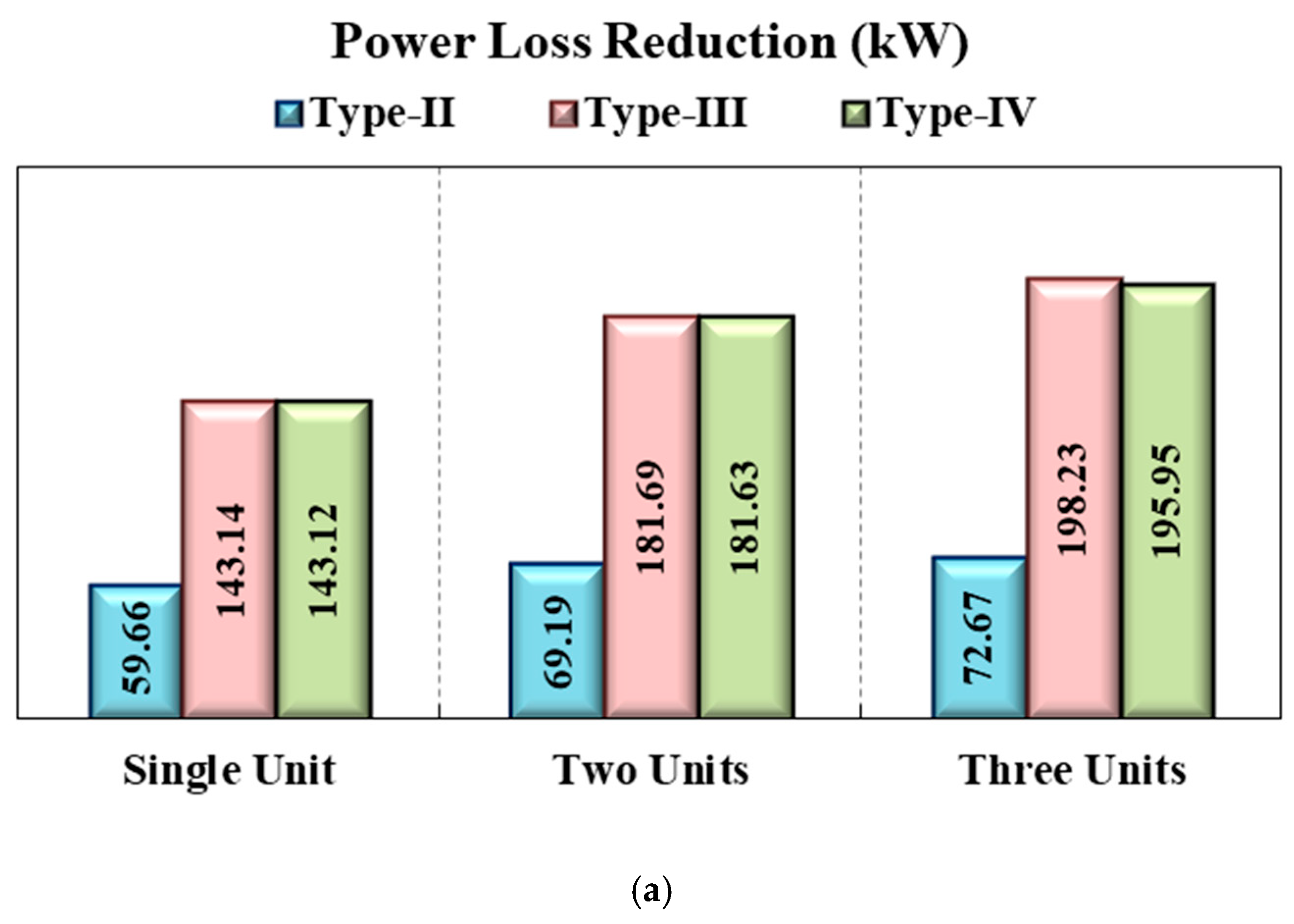
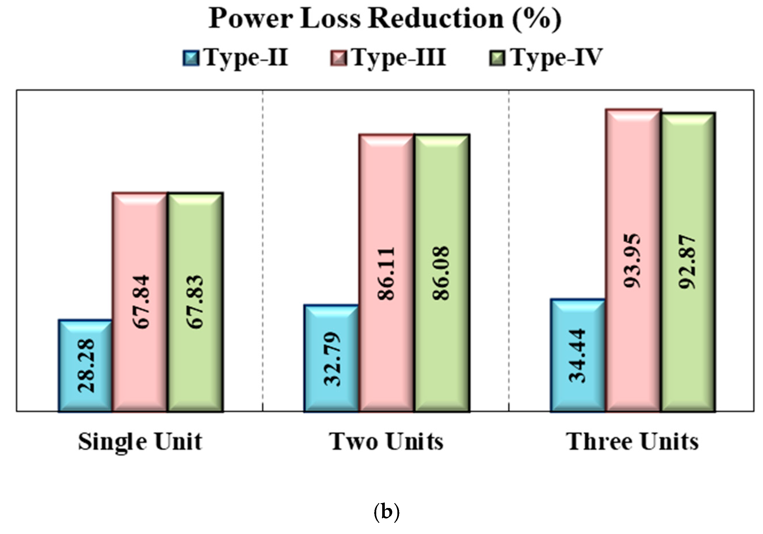
- Optimally allocating a single type-II DG unit reduces the power losses by 28.275% compared to the base case (when no DG is connected) and improves the voltage profile by 0.0127 p.u.
- ii.
- Including a second type-II DG unit optimally enhances power loss reduction by 4.517% and improves the voltage profile by 0.0138 p.u. compared to the first case.
- iii.
- Optimally incorporating three type-II DG units achieves a maximum loss reduction of 34.441% and a voltage profile improvement of 0.0273 p.u. compared to the base case. The graphical representation of obtained power losses and loss reductions are presented in Figure 7.
- iv.
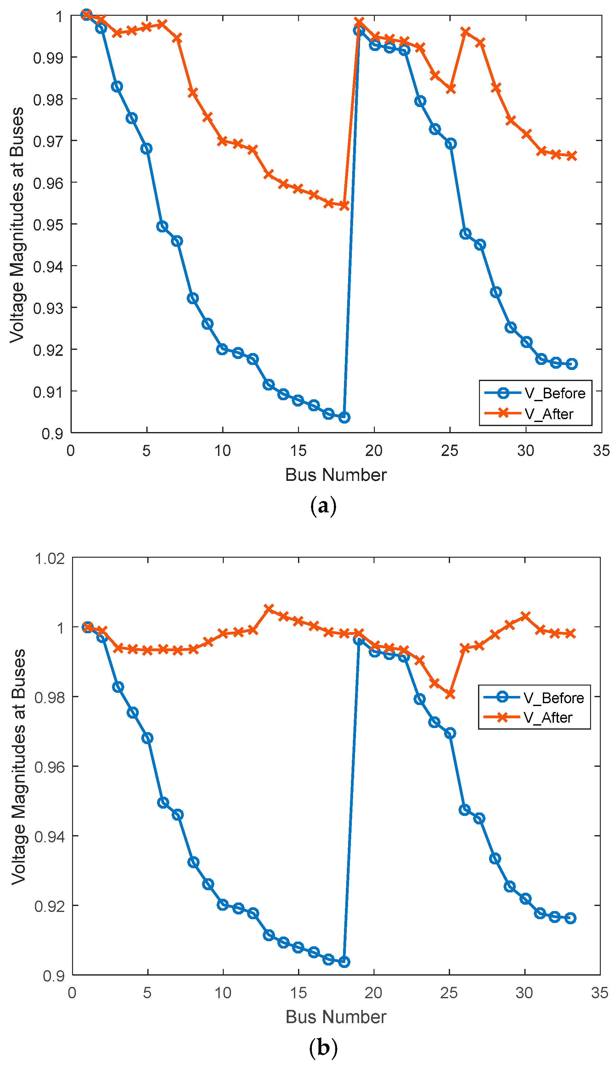
- Adding more DG units indicates a diminishing return effect, as the improvement margin for both power losses and voltage profile continues to reduce. It is also evident from Figure 8b,c, which appear nearly identical; however, a close examination reveals that case A2 exhibits a slight dominance in voltages for buses 30–33. For case A2, voltages on these buses lie close to 0.95 p.u., compared to approximately 0.94 p.u. in case A3. While case A3 attained a marginally higher minimum bus voltage, case A2 proved more beneficial overall on average, as more buses experienced significant voltage improvement.
- v.
- Before and after optimally allocating type-II DGs in the IEEE 33-bus test system, bus # 18 remains the weakest bus in the IEEE 33-bus test system, maybe because of its distant location from the grid station.
5.2. Results for Type-III DG (Supply Active and Reactive Powers)
| DG Type | PDG Active power output | QDG Reactive power output | |
| Type-III | (11) |
- i.
- Optimally allocating a single type-III DG unit reduces the power losses by 67.862% compared to the base case (when no DG is connected) and improves the voltage profile by 0.0545 p.u.
- ii.
- Including a second type-III DG unit optimally enhances the power loss reduction by 18.271% and improves the voltage profile by 0.0221 p.u. compared to the first case.
- iii.
- Optimally incorporating three type-III DG units achieves the maximum loss reduction of 93.948% and voltage profile improvement of 9.792% compared to the base case.
- iv.
- Similar to type-II DGs, adding more type-III DGs diminishes the return effect as the improvement margin for both power losses and voltage profile keeps reducing.
- v.
- Before allocating type-III DGs, bus # 18 was the weakest bus in the IEEE 33-bus test system, which switches between buses 8, 18, and 25 after optimally allocating the single and multiple units of type-III DGs.
- vi.
- Optimally allocating two type-III DG units enhances power loss reduction compared to a single DG unit allocation while requiring less active and reactive power from DGs. It signifies the impact of selecting proper locations for DGs’ placement. Choosing the proper DG location can significantly drop the DG’s power output, thus achieving better techno-economic performance of the distribution network.
5.3. Results for Type-IV DG (Supply Active Power and Dynamically Adjust Reactive Power)
| DG Type | PDG Active power output | QDG Reactive power output | |
| Type-IV | (12) |
- i.
- Optimally allocating three type-IV DG units achieves the maximum loss reduction of 92.866% compared to the base case.
- ii.
- Similar to the two DG types previously studied, adding more type-IV DGs diminishes the improvement margin for power losses and voltage profile.
- iii.
- Before allocating type-IV DGs, bus # 18 was the weakest bus in the IEEE 33-bus test system, which switches between buses 18 and 25 after optimally allocating type-IV DGs.
- iv.
- Injecting active power is more effective than reactive power in enhancing the distribution network performance.
- i.
- Type-III and type-IV DGs are more effective in enhancing the performance of power distribution networks as both DGs can adjust power factors.
- ii.
- Type-IV DGs slightly lag behind type-III DGs in attaining the same level of loss reduction despite both being capable of adjusting power factors. However, this lag stems from type-IV DG’s broader operating power factor range, which adds complexity to reaching equivalent performance.
- iii.
- Type-II DG, capable of injecting only reactive power, is the least effective among the four studied DG types in improving the distribution network performance.
- iv.
- One common observation for all DG types is that the optimal allocation of two units of each DG type is most effective in the obtained loss reduction to DGs’ power injection ratio.
5.4. Results for Combined DG Allocation
| Case 1 (A1B1C1): | Type-II DGs = 1, | Type-III DGs = 1, | Type-IV DGs = 1 |
| Case 2 (A1B1C2): | Type-II DGs = 1, | Type-III DGs = 1, | Type-IV DGs = 2 |
| Case 3 (A1B1C3): | Type-II DGs = 1, | Type-III DGs = 1, | Type-IV DGs = 3 |
| Case 4 (A1B2C1): | Type-II DGs = 1, | Type-III DGs = 2, | Type-IV DGs = 1 |
| Case 5 (A1B2C2): | Type-II DGs = 1, | Type-III DGs = 2, | Type-IV DGs = 2 |
| Case 6 (A1B2C3): | Type-II DGs = 1, | Type-III DGs = 2, | Type-IV DGs = 3 |
| Case 7 (A1B3C1): | Type-II DGs = 1, | Type-III DGs = 3, | Type-IV DGs = 1 |
| Case 8 (A1B3C2): | Type-II DGs = 1, | Type-III DGs = 3, | Type-IV DGs = 2 |
| Case 9 (A1B3C3): | Type-II DGs = 1, | Type-III DGs = 3, | Type-IV DGs = 3 |
| Case 10 (A2B1C1): | Type-II DGs = 2, | Type-III DGs = 1, | Type-IV DGs = 1 |
| Case 11 (A2B1C2): | Type-II DGs = 2, | Type-III DGs = 1, | Type-IV DGs = 2 |
| Case 12 (A2B1C3): | Type-II DGs = 2, | Type-III DGs = 1, | Type-IV DGs = 3 |
| Case 13 (A2B2C1): | Type-II DGs = 2, | Type-III DGs = 2, | Type-IV DGs = 1 |
| Case 14 (A2B2C2): | Type-II DGs = 2, | Type-III DGs = 2, | Type-IV DGs = 2 |
| Case 15 (A2B2C3): | Type-II DGs = 2, | Type-III DGs = 2, | Type-IV DGs = 3 |
| Case 16 (A2B3C1): | Type-II DGs = 2, | Type-III DGs = 3, | Type-IV DGs = 1 |
| Case 17 (A2B3C2): | Type-II DGs = 2, | Type-III DGs = 3, | Type-IV DGs = 2 |
| Case 18 (A2B3C3): | Type-II DGs = 2, | Type-III DGs = 3, | Type-IV DGs = 3 |
| Case 19 (A3B1C1): | Type-II DGs = 3, | Type-III DGs = 1, | Type-IV DGs = 1 |
| Case 20 (A3B1C2): | Type-II DGs = 3, | Type-III DGs = 1, | Type-IV DGs = 2 |
| Case 21 (A3B1C3): | Type-II DGs = 3, | Type-III DGs = 1, | Type-IV DGs = 3 |
| Case 22 (A3B2C1): | Type-II DGs = 3, | Type-III DGs = 2, | Type-IV DGs = 1 |
| Case 23 (A3B2C2): | Type-II DGs = 3, | Type-III DGs = 2, | Type-IV DGs = 2 |
| Case 24 (A3B2C3): | Type-II DGs = 3, | Type-III DGs = 2, | Type-IV DGs = 3 |
| Case 25 (A3B3C1): | Type-II DGs = 3, | Type-III DGs = 3, | Type-IV DGs = 1 |
| Case 26 (A3B3C2): | Type-II DGs = 3, | Type-III DGs = 3, | Type-IV DGs = 2 |
| Case 27 (A3B3C3): | Type-II DGs = 3, | Type-III DGs = 3, | Type-IV DGs = 3 |
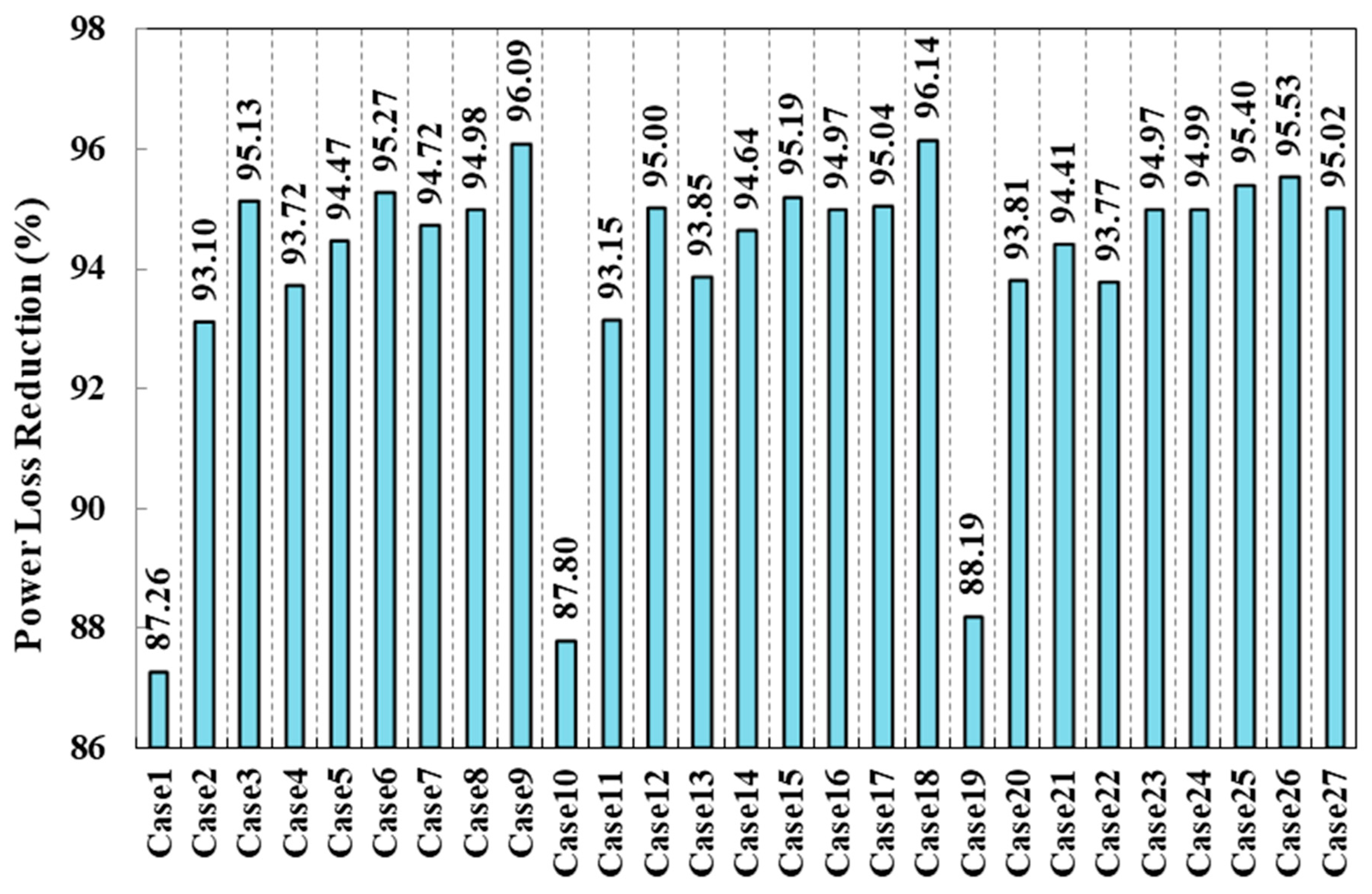
- i.
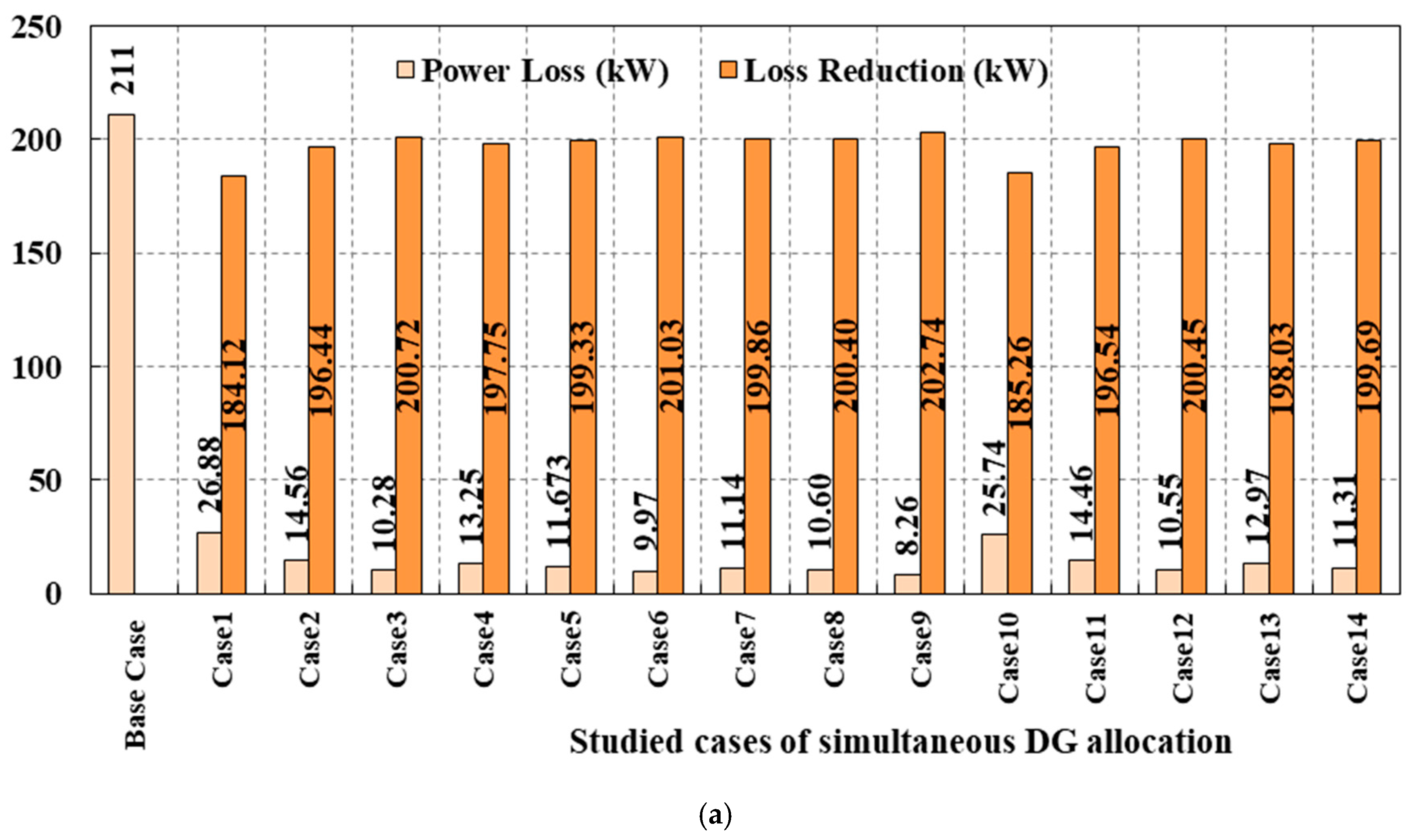
- The minimum power loss reduction of 87.262% is obtained by jointly allocating a single unit of each DG type, i.e., Case 1 (A1B1C1).
- ii.
- The highest power loss reduction of 96.139% is obtained by allocating two type-II DGs and three units of type-III and type-IV DGs, i.e., Case 18.
- iii.
- Case 14 is the worst regarding the power loss reduction to the DGs’ active power injection ratio, with a value of 0.059.
- iv.
- Case 19 is the best regarding the power loss reduction to the DGs’ active power injection ratio, with a value of 0.097.
- v.
- Adding more DG units is not always practical, as it may diminish the return effect of DG investment. It is evident from Cases 12 (B2C1D3) and 24 (A3B2C3) as both achieve the same level of loss reduction. However, Case 24 requires two additional DG units (one type-II DG and one type-III DG), which do not contribute to further improving the overall performance of the distribution network.
- vi.
- Adding type-III DGs with a corresponding decrement in the number of type-IV DGs does not significantly impact power losses. This phenomenon can be observed in Cases 12 and 16.
- vii.
- Integrating additional type-II DGs alongside type-III and IV DGs may be detrimental as the excessive reactive power injection can degrade network performance rather than improve it.
- viii.
- Bus # 18 is the commonly observed weakest bus in the IEEE 33-bus test system, sometimes switching to buses 25, 30, and 32. However, buses 18 and 25 are the commonly observed weakest buses after optimally allocating the DG units.
- ix.
- Among individual allocation of type-II to type-IV DG types, the highest loss reduction of 93.948% was observed while deploying three type-III units. In contrast, when the proposed DG types are allocated simultaneously, 18 out of 27 cases (Cases 3, 5–9, 12, 14–18, 21, 23–27) outperformed this best case of individual allocation by significant margins, thus highlighting the effectiveness of jointly allocating proposed DG types.
- x.
- Among the 18 best cases of simultaneous allocation of DG units that outperformed the best case of individual allocation, three cases (Cases 3, 7, and 8) attain more reductions in power losses by employing lower total active and reactive power capacities.
5.5. Effectiveness of Proposed Approach Against Existing Studies
6. Conclusions
7. Limitations and Future Research Directions
Author Contributions
Funding
Institutional Review Board Statement
Informed Consent Statement
Data Availability Statement
Conflicts of Interest
References
- Leghari, Z.H.; Hassan, M.Y.; Said, D.M.; Memon, Z.A.; Hussain, S. An efficient framework for integrating distributed generation and capacitor units for simultaneous grid-connected and islanded network operations. Int. J. Energy Res. 2021, 45, 1–39. [Google Scholar] [CrossRef]
- US Energy Information Administration. World Energy Demand and Economic Outlook. In International Energy Outlook; US Energy Information Administration: Washington, DC, USA, 2016; Volume 484, pp. 7–18. [Google Scholar]
- IEA. Distributed Generation in Liberalised Electricity Markets; IEA: Paris, France, 2002. [Google Scholar]
- Pesaran, H.A.M.; Huy, P.D.; Ramachandaramurthy, V.K. A review of the optimal allocation of distributed generation: Objectives, constraints, methods, and algorithms. Renew. Sustain. Energy Rev. 2017, 75, 293–312. [Google Scholar] [CrossRef]
- Sulaima, M.F.; Mohamad, M.F.; Jali, M.H.; Bukhari, W.M.; Baharom, M.F. A comparative study of optimization methods for 33kV distribution network feeder reconfiguration. Int. J. Appl. Eng. Res. 2014, 9, 1169–1182. [Google Scholar]
- Leghari, Z.H.; Kumar, M.; Shaikh, P.H.; Kumar, L.; Tran, Q.T. A critical review of optimization strategies for simultaneous integration of distributed generation and capacitor banks in power distribution networks. Energies 2022, 15, 8258. [Google Scholar] [CrossRef]
- Wang, S.; Li, Z.; Golkar, M.J. Optimum placement of distributed generation resources, capacitors and charging stations with a developed competitive algorithm. Heliyon 2024, 10, e26194. [Google Scholar] [CrossRef]
- Basu, M.; Jena, C.; Khan, B.; Ali, A.; Khurshaid, T. Optimal sizing and placement of capacitors in the isolated microgrid throughout the day considering the demand response program. Front. Energy Res. 2024, 12, 1346330. [Google Scholar] [CrossRef]
- Kannemadugu, R.P.; Adhimoorthy, V.; Devi, A.L.; Asokan, K. Optimal allocation of combined DG and DSTATCOM for improving voltage stability and economical benefits of distribution system. Int. Res. J. Adv. Eng. Hub 2024, 2, 18–25. [Google Scholar] [CrossRef]
- Pratap, A.; Tiwari, P.; Maurya, R.; Singh, B. Cheetah optimization algorithm for simultaneous optimal network reconfiguration and allocation of DG and DSTATCOM with electric vehicle charging station. Serbian J. Electr. Eng. 2024, 21, 1–37. [Google Scholar] [CrossRef]
- Rehman, N.; Mufti, M.D.; Gupta, N. Optimal location of electric vehicles in a wind integrated distribution system using reptile search algorithm. Distrib. Gener. Altern. Energy J. 2023, 38, 141–168. [Google Scholar] [CrossRef]
- Borousan, F.; Hamidan, M.A. Distributed power generation planning for distribution network using chimp optimization algorithm in order to reliability improvement. Electr. Power Syst. Res. 2023, 217, 109109. [Google Scholar] [CrossRef]
- Selim, S.O.; Selim, A.; Kamel, S. Power Loss Minimization Using Optimal Allocation of DGs Based on Wild Horse Optimizer. In Proceedings of the 23rd International Middle East Power Systems Conference (MEPCON), Cairo, Egypt, 13–15 December 2022. [Google Scholar]
- Ali, M.H.; Kamel, S.; Hassan, M.H.; Tostado-Véliz, M.; Zawbaa, H.M. An improved wild horse optimization algorithm for reliability based optimal DG planning of radial distribution networks. Energy Rep. 2022, 8, 582–604. [Google Scholar] [CrossRef]
- Kawambwa, S.; Hamisi, N.; Mafole, P.; Kundaeli, H. A cloud model based symbiotic organism search algorithm for DG allocation in radial distribution network. Evol. Intell. 2022, 15, 545–562. [Google Scholar] [CrossRef]
- Salkuti, S.R. Optimal allocation of DG D-STATCOM in a distribution system using evolutionary based Bat algorithm. Int. J. Adv. Comput. Sci. Appl. 2021, 12, 4. [Google Scholar] [CrossRef]
- Chakraborty, S.; Verma, S.; Salgotra, A.; Elavarasan, R.M.; Elangovan, D.; Mihet-Popa, L. Solar-based DG allocation using Harris Hawks Optimization while considering practical aspects. Energies 2021, 14, 5206. [Google Scholar] [CrossRef]
- Fathy, A.; Yousri, D.; Abdelaziz, A.Y.; Ramadan, H.S. Robust approach based chimp optimization algorithm for minimizing power loss of electrical distribution networks via allocating distributed generators. Sustain. Energy Technol. Assess. 2021, 47, 101359. [Google Scholar] [CrossRef]
- Nguyen, T.T.; Nguyen, T.T.; Nguyen, N.A.; Duong, T.L. A novel method based on coyote algorithm for simultaneous network reconfiguration and distribution generation placement. Ain Shams Eng. J. 2021, 12, 665–676. [Google Scholar] [CrossRef]
- Chippagiri, S.S.; Pemmada, S.; Patne, N. Distribution network reconfiguration and distributed generation injection using improved Elephant Herding Optimization. In Proceedings of the IEEE First International Conference on Smart Technologies for Power, Energy and Control (STPEC), Nagpur, India, 25–26 September 2020. [Google Scholar]
- Jalili, A.; Taheri, B. Optimal sizing and sitting of distributed generations in power distribution networks using firefly algorithm. Technol. Econ. Smart Grids Sustain. Energy 2020, 5, 1–14. [Google Scholar] [CrossRef]
- Ton, T.N.; Nguyen, T.; Truong, A.; Vu, T.P. Optimal location and size of distributed generators in an electric distribution system based on a novel metaheuristic algorithm. Eng. Technol. Appl. Sci. Res. 2020, 10, 5325–5329. [Google Scholar] [CrossRef]
- Boukaroura, A.; Slimani, L.; Bouktir, T. Optimal placement and sizing of multiple renewable distributed generation units considering load variations via dragonfly optimization algorithm. Iran. J. Electr. Electron. Eng. 2020, 16, 353–362. [Google Scholar]
- Zakaria, Y.Y.; Swief, R.; El-Amary, N.H.; Ibrahim, A.M. Optimal distributed generation allocation and sizing using genetic and ant colony algorithms. J. Phys. Conf. Ser. 2020, 1447, 012023. [Google Scholar] [CrossRef]
- Rao, R.V.; Savsani, V.J.; Balic, J. Teaching-learning-based optimization algorithm for unconstrained and constrained real-parameter optimization problems. Eng. Optim. 2012, 44, 1447–1462. [Google Scholar] [CrossRef]
- Rao, R.V. Jaya: A simple and new optimization algorithm for solving constrained and unconstrained optimization problems. Int. J. Ind. Eng. Comput. 2016, 7, 19–34. [Google Scholar]
- Rao, R.V.; Waghmare, G.G. A new optimization algorithm for solving complex constrained design optimization problems. Eng. Optim. 2017, 49, 60–83. [Google Scholar] [CrossRef]
- El-Ela, A.A.A.; El-Sehiemy, R.A.; Abbas, A.S. Optimal placement and sizing of distributed generation and capacitor banks in distribution systems using Water Cycle Algorithm. IEEE Syst. J. 2018, 12, 3629–3636. [Google Scholar] [CrossRef]
- Saonerkar, A.K.; Bagde, B.Y. Optimized DG placement in radial distribution system with reconfiguration and capacitor placement using genetic algorithm. In Proceedings of the 2014 IEEE International Conference on Advanced Communications, Control and Computing Technologies, Ramanathapuram, India, 8–10 May 2014; pp. 1077–1083. [Google Scholar]
- Venkatesan, C.; Kannadasan, R.; Alsharif, M.H.; Kim, M.K.; Nebhen, J. A novel multiobjective hybrid technique for siting and sizing of distributed generation and capacitor banks in radial distribution systems. Sustainability 2021, 13, 3308. [Google Scholar] [CrossRef]
- Zhai, X.; Li, Z.; Li, Z.; Xue, Y.; Chang, X.; Su, J.; Jin, X.; Wang, P.; Sun, H. Risk-averse energy management for integrated electricity and heat systems considering building heating vertical imbalance: An asynchronous decentralized approach. Appl. Energy 2025, 383, 125271. [Google Scholar] [CrossRef]
- Zhang, H.; Li, Z.; Xue, Y.; Chang, X.; Su, J.; Wang, P.; Guo, Q.; Su, H. A Stochastic Bi-level Optimal Allocation Approach of Intelligent Buildings Considering Energy Storage Sharing Services. IEEE Trans. Consum. Electron. 2024, 70, 5142–5153. [Google Scholar] [CrossRef]
- Gupta, B. Power System; S. Chand Publishing: Noida, India, 2008. [Google Scholar]
- Dixon, J.; Moran, L.; Rodriguez, J.; Domke, R. Reactive power compensation technologies: State-of-the-art review. Proc. IEEE 2005, 93, 2144–2164. [Google Scholar] [CrossRef]


| Ref. # | Objective (s) | Technique(s) | DG Types | Bus System(s) | |||||
|---|---|---|---|---|---|---|---|---|---|
| Technical | Economic | Environmental | I | II | III | IV | |||
| [7] | ✓ | CSO | ✓ | ✓ | ✓ | 69 | |||
| [8] | QOFCEP/FCEP/EP | ✓ | ✓ | 33, 69, 118 | |||||
| [9] | ✓ | GTO | ✓ | ✓ | 69 | ||||
| [10] | ✓ | ✓ | CO | ✓ | ✓ | 33, 136 | |||
| [11] | ✓ | RSA | ✓ | ✓ | 33, 69 | ||||
| [12] | ✓ | ChOA | ✓ | 119 | |||||
| [13] | ✓ | WHO | ✓ | 33, 69 | |||||
| [14] | ✓ | IWHO | ✓ | ✓ | 33, 69, 119 | ||||
| [15] | ✓ | ✓ | SOS | ✓ | ✓ | 69 | |||
| [16] | ✓ | EBA | ✓ | ✓ | 33, 85 | ||||
| [17] | ✓ | HHO | ✓ | 33, 69 | |||||
| [18] | ✓ | ChOA | ✓ | ✓ | 33, 69 | ||||
| [19] | ✓ | COA | ✓ | 69, 119 | |||||
| [20] | ✓ | IEHO | ✓ | 33, 69, 119 | |||||
| [21] | ✓ | FO | ✓ | ✓ | ✓ | 33, 69 | |||
| [22] | ✓ | COA | ✓ | 33 | |||||
| [23] | ✓ | DOA | ✓ | 33, 69 | |||||
| [24] | ✓ | ACO, GA | ✓ | ✓ | ✓ | 59 | |||
| Case # | DG Size (MVAR), Location (Bus #) | Total DG Capacity | Power Loss (kW) | Loss Reduction (%) | Vmin (p.u.), Bus # | |
|---|---|---|---|---|---|---|
| P MW | Q MVAR | |||||
| Base Case | - | - | - | 211 | - | 0.9038 (18) |
| Case A1 | 1.2580 (30) | - | 1.2580 | 151.34 | 28.275 | 0.9165 (18) |
| Case A2 | 0.4651 (12) | - | 1.5284 | 141.81 | 32.792 | 0.9303 (18) |
| 1.0633 (30) | ||||||
| Case A3 | 0.4144 (13) | - | 1.9082 | 138.33 | 34.441 | 0.9311 (18) |
| 0.4934 (24) | ||||||
| 1.0004 (30) | ||||||
| Case # | DG Size (MVA), Power Factor, Location (Bus #) | Total DG Capacity | Power Loss (kW) | Loss Reduction (%) | Vmin (p.u.), Bus # | |
|---|---|---|---|---|---|---|
| P MW | Q MVAR | |||||
| Base Case | - | - | - | 211 | - | 0.9038 (18) |
| Case B1 | 3.1060, 0.824 lag, (6) | 2.5583 | 1.7612 | 67.862 | 67.838 | 0.9583 (18) |
| Case B2 | 0.9268, 0.883 lag, (13) | 2.0588 | 1.3656 | 29.311 | 86.109 | 0.9804 (25) |
| 1.5506, 0.800 lag, (30) | ||||||
| Case B3 | 0.8672, 0.883 lag, (13) | 2.9660 | 1.8402 | 12.769 | 93.948 | 0.9923 (8) |
| 1.1826, 0.879 lag, (24) | ||||||
| 1.4502, 0.801 lag, (30) | ||||||
| Case # | DG Size (MVA), Power Factor, Location (Bus #) | Total DG Capacity | Power Loss (kW) | Loss Reduction (%) | Vmin (p.u.), Bus # | |
|---|---|---|---|---|---|---|
| P MW | Q MVAR | |||||
| Base Case | - | - | - | 211 | - | 0.9038 (18) |
| Case C1 | 3.1059, 0.830 lag, (6) | 2.5779 | 1.7324 | 67.878 | 67.830 | 0.9545 (18) |
| Case C2 | 0.9241, 0.868 lag, (13) | 2.0277 | 1.3780 | 29.368 | 86.082 | 0.9807 (25) |
| 1.5320, 0.800 lag, (30) | ||||||
| Case C3 | 0.7655, 0.808 lag, (14) | 2.8842 | 2.1503 | 15.052 | 92.866 | 0.9427 (18) |
| 1.2042, 0.800 lag, (24) | ||||||
| 1.6279, 0.800 lag, (30) | ||||||
| Case # | DG Size, Power Factor, Location | Total DG Capacity | Power Loss (kW) | Loss Reduction (%) | Vmin (p.u.), Bus # | |||
|---|---|---|---|---|---|---|---|---|
| Type-II MVAR (Bus #) | Type-III MVA, pf (Bus #) | Type-IV MVA, pf (Bus #) | P MW | Q MVAR | ||||
| Base Case | - | - | 211 | - | 0.9038 (18) | |||
| Case 1 A1B1C1 | 0.2959 (25) | 1.0574, 0.894 lead, (12) | 1.5013, 0.812 lead (30) | 2.1645 | 1.6456 | 26.877 | 87.262 | 0.9814 (25) |
| Case 2 A1B1C2 | 0.6059 (31) | 1.0708, 0.867 lead, (10) | 1.3295, 0.918 lead, (24) | 3.2043 | 1.9429 | 14.559 | 93.100 | 0.9744 (18) |
| - | - | 0.95413 0.957 lead (30) | ||||||
| Case 3 A1B1C3 | 0.2609 (29) | 0.8654, 0.863 lead, (32) | 0.8432, 0.909 lead, (7) | 2.9301 | 1.5493 | 10.279 | 95.128 | 0.9826 (25) |
| - | - | 0.6264, 0.908 lead, (14) | ||||||
| - | - | 0.8805, 0.963 lead, (25) | ||||||
| Case 4 A1B2C1 | 0.0760, (33) | 0.8931, 0.865 lead, (14) | 1.0627, 0.853 lead, (24) | 2.8244 | 1.8281 | 13.254 | 93.718 | 0.9816 (18) |
| - | 1.3689, 0.837 lead, (30) | - | ||||||
| Case 5 A1B2C2 | 0.5209 (31) | 1.0134, 0.902 lead, (6) | 0.7018, 0.821 lead, (13) | 2.6987 | 1.9720 | 11.673 | 94.468 | 0.9918 (30) |
| - | 0.6864, 0.863 lead, (24) | 0.6713, 0.919 lead, (31) | ||||||
| Case 6 A1B2C3 | 0.4836 (30) | 1.2287, 0.890 lead, (5) | 0.3208, 0.984 lead, (11) | 3.3516 | 2.2125 | 9.972 | 95.274 | 0.9531 (18) |
| - | 0.8911, 0.831 lead, (25) | 0.6443, 0.866 lead, (14) | ||||||
| - | - | 0.7078, 0.910 lead, (33) | ||||||
| Case 7 A1B3C1 | 0.6029 (30) | 0.8938, 0.904 lead, (6) | 0.6731, 0.989 lead, (31) | 2.8289 | 1.6970 | 11.136 | 94.722 | 0.9785 (32) |
| - | 0.7581, 0.932 lead, (13) | - | ||||||
| - | 0.7312, 0.888 lead, (24) | - | ||||||
| Case 8 A1B3C2 | 0.7119 (30) | 0.6690, 0.899 lead, (9) | 0.3008, 0.917 lead, (18) | 2.6070 | 1.7686 | 10.596 | 94.978 | 0.9582 (18) |
| - | 0.1545, 0.976 lead, (10) | 0.7436, 0.831 lead, (25) | ||||||
| - | 0.9808, 0.980 lead, (31) | - | ||||||
| Case 9 A1B3C3 | 0.5256 (30) | 0.8208, 0.859 lead, (6) | 0.0690, 0.998 lead, (4) | 2.8957 | 2.112 | 8.258 | 96.086 | 0.9662 (18) |
| - | 0.5684, 0.876 lead, (14) | 0.9112, 0.897 lead, (24) | ||||||
| - | 0.5871, 0.853 lead, (33) | 0.3538, 0.866 lead, (29) | ||||||
| Case 10 A2B1C1 | 0.51133 (24) | 0.9647, 0.922 lead, (14) | 1.1426, 0.95 lag, (30) | 1.9747 | 1.9254 | 25.744 | 87.799 | 0.9880 (25) |
| 1.3966 (30) | - | - | ||||||
| Case 11 A2B1C2 | 0.3822 (28) | 1.2327, 0.872 lead, (30) | 0.8169, 0.929 lead, (15) | 2.8846 | 1.8698 | 14.463 | 93.146 | 0.9602 (18) |
| 0.3103 (33) | - | 1.0851 0.968 lead, (25) | ||||||
| Case 12 A2B1C3 | 0.5292 (6) | 0.9776, 0.850 lead, (25) | 0.5656, 0.971 lead, (13) | 2.8741 | 2.1430 | 10.552 | 94.999 | 0.9523 (18) |
| 0.6886 (30) | - | 0.6785, 0.991 lead, (26) | ||||||
| - | - | 0.7989, 0.973 lead, (32) | ||||||
| Case 13 A2B2C1 | 0.1991 (5) | 0.9318 0.858 lead, (12) | 1.1784, 0.868 lead, (24) | 2.9711 | 2.1283 | 12.968 | 93.854 | 0.9315 (18) |
| 0.2662 (32) | 1.2957, 0.889 lead, (30) | - | ||||||
| Case 14 A2B2C2 | 0.2169 (22) | 0.72734 0.891 lead, (13) | 0.6687, 0.854 lead, (6) | 3.3866 | 2.0309 | 11.306 | 94.642 | 0.9505 (18) |
| 0.4074 (28) | 1.0636, 0.852 lead, (31) | 1.2734, 0.991 lead, (24) | ||||||
| Case 15 A2B2C3 | 0.5957 (6) | 0.6963, 0.912 lead, (24) | 0.7165, 0.955 lead, (5) | 3.1166 | 2.0560 | 10.143 | 95.193 | 0.9556 (18) |
| 0.4530 (30) | 0.8064, 0.857 lead, (33) | 0.6742, 0.934 lead, (13) | ||||||
| - | - | 0.4969, 0.958 lag, (26) | ||||||
| Case 16 A2B3C1 | 0.3205 (29) | 0.7836, 0.972 lead, (14) | 0.9438, 0.926 lead, (31) | 3.1117 | 1.7513 | 10.608 | 94.973 | 0.9501 (18) |
| 0.1447 (33) | 0.8204, 0.913 lead, (25) | - | ||||||
| - | 0.8354, 0.870 lead, (26) | - | ||||||
| Case 17 A2B3C2 | 0.4059 (4) | 0.3489, 0.837 lead, (9) | 0.8880, 0.9 lead, (25) | 2.7356 | 2.1880 | 10.466 | 95.040 | 0.9492 (18) |
| 0.8480 (30) | 0.8439, 0.928 lead, (15) | 0.488, 0.886 lag, (30) | ||||||
| - | 0.5057, 0.848 lead, (33) | - | ||||||
| Case 18 A2B3C3 | 0.1356, (22) | 0.1857, 0.886 lag, (10) | 0.4706, 0.831 lead, (7) | 3.008 | 2.2166 | 8.146 | 96.139 | 0.9799 (25) |
| 0.2828, (33) | 0.5984, 0.802 lead, (16) | 0.7556, 0.885 lead, (25) | ||||||
| - | 0.9284, 0.821 lead, (30) | 0.5814, 0.932 lead, (27) | ||||||
| Case 19 A3B1C1 | 0.5301 (3) | 1.3323, 0.824 lead, (30) | 0.8840, 0.925 lead, (14) | 1.9154 | 1.6184 | 24.926 | 88.187 | 0.9768 (18) |
| 0.3425 (25) | - | - | ||||||
| 0.1850 (33) | - | - | ||||||
| Case 20 A3B1C2 | 0.3620 (7) | 1.2458, 0.938 lead, (30) | 0.8314, 0.937 lead, (13) | 2.5498 | 2.1619 | 13.072 | 93.805 | 0.9880 (25) |
| 0.1149 (21) | - | 0.7127, 0.845 lead, (25) | ||||||
| 0.5816 (30) | - | - | ||||||
| Case 21 A3B1C3 | 0.2203 (2) | 0.8253, 0.853 lead, (25) | 0.7094, 0.922 lead, (10) | 2.7814 | 2.0629 | 11.802 | 94.407 | 0.9199 (18) |
| 0.9751 (30) | - | 0.7928, 0.925 lead, (26) | ||||||
| 0.1753 (33) | - | 0.7580, 0.91 lag, (30) | ||||||
| Case 22 A3B2C1 | 0.2691 (16) | 0.8288, 0.966 lead, (12) | 1.0763, 0.911 lead, (30) | 2.9393 | 1.8278 | 13.139 | 93.773 | 0.9730 (30) |
| 0.3051 (29) | 1.2581, 0.920 lead, (24) | - | ||||||
| 0.1041 (31) | - | - | ||||||
| Case 23 A3B2C2 | 0.0035 (9) | 0.9704, 0.886 lead, (24) | 0.6531, 0.855 lead, (9) | 2.9871 | 2.0842 | 10.607 | 94.973 | 0.9381 (18) |
| 0.0616 (13) | 1.4235, 0.832 lead, (30) | 0.4133, 0.929 lead, (15) | ||||||
| 0.2890 (33) | - | - | ||||||
| Case 24 A3B2C3 | 0.1416 (9) | 0.1730, 0.984 lead, (3) | 0.4626, 0.942 lead, (6) | 2.9658 | 1.9759 | 10.556 | 94.997 | 0.9526 (18) |
| 0.2719 (30) | 1.0951, 0.922 lead, (30) | 0.5400, 0.878 lead, (14) | ||||||
| 0.3548 (33) | - | 0.9394, 0.933 lead, (24) | ||||||
| Case 25 A3B3C1 | 0.1641 (11) | 0.6383, 0.884 lead, (14) | 0.7585, 0.837 lead, (30) | 2.8055 | 2.0917 | 9.713 | 95.397 | 0.9325 (18) |
| 0.3699 (33) | 0.8436, 0.887 lead, (25) | - | ||||||
| 0.0772 (33) | 0.9375, 0.915 lead, (26) | - | ||||||
| Case 26 A3B3C2 | 0.2833 (2) | 0.4504, 0.894 lead, (16) | 0.0621, 0.962 lag, (10) | 2.9058 | 2.0944 | 9.425 | 95.533 | 0.9777 (32) |
| 0.4713 (30) | 1.0881, 0.905 lead, (24) | 0.5725, 0.929 lead, (12) | ||||||
| 0.1152 (32) | 0.9960, 0.930 lead, (30) | - | ||||||
| Case 27 A3B3C3 | 1.0583 (2) | 1.2685, 0.914 lead, (24) | 0.1927, 0.955 lead, (6) | 2.9938 | 1.8568 | 10.518 | 95.015 | 0.9927 (25) |
| 0.4019 (27) | 0.6264, 0.803 lead, (30) | 0.7437, 0.909 lead, (13) | ||||||
| 0.1933 (33) | 0.2601, 0.814 lead, (32) | 0.1471, 0.822 lag, (33) | ||||||
| No. of Type-III DG Units | ||||||
|---|---|---|---|---|---|---|
| 1 | 2 | 3 | ||||
| No. of Type-II DG units | 1 | 184.123 kW 87.262% | 197.746 kW 93.718% | 199.864 kW 94.722% | 1 | No. of Type-IV DG units |
| 196.441 kW 93.100% | 199.327 kW 94.468% | 200.404 kW 94.978% | 2 | |||
| 200.721 kW 95.128% | 201.028 kW 95.274% | 202.742 kW 96.086% | 3 | |||
| 2 | 185.256 kW 87.799% | 198.032 kW 93.854% | 200.392 kW 94.973% | 1 | ||
| 196.537 kW 93.146% | 199.694 kW 94.642% | 200.534 kW 95.040% | 2 | |||
| 200.448 kW 94.999% | 200.857 kW 95.193% | 202.854 kW 96.139% | 3 | |||
| 3 | 186.074 kW 88.187% | 197.861 kW 93.773% | 201.287 kW 95.397% | 1 | ||
| 197.928 kW 93.805% | 200.393 kW 94.973% | 201.575 kW 95.533% | 2 | |||
| 199.198 kW 94.407% | 200.434 kW 94.992% | 200.518 kW 95.015% | 3 | |||
| Technique | Total DG Capacity | No. of Existing DG Units | No. of Proposed DG Units | Total No. of DG Units | Power Loss Reduction (%) | ||||||
|---|---|---|---|---|---|---|---|---|---|---|---|
| P (MW) | Q (MVAR) | I | II | III | IV | II | III | IV | |||
| WCA [28] | 2.576 | 1.565 | 3 | 3 | - | - | 6 | 87.82 | |||
| GA [29] | 1 | 1.8 | 3 | 3 | - | - | 6 | 64.85 | |||
| Proposed Case 1 | 2.165 | 1.646 | 1 | 1 | 1 | 3 | 87.26 | ||||
| Proposed Case 19 | 1.9154 | 1.6184 | 3 | 1 | 1 | 5 | 88.19 | ||||
| EGWO-PSO [30] | 2.873 | 2.241 | 3 | 3 | - | - | 6 | 92.52 | |||
| Proposed Case 7 | 2.829 | 1.697 | 1 | 3 | 1 | 5 | 94.72 | ||||
| WCA [28] | 3.626 | 1.1798 | - | 3 | 3 | - | 6 | 90.21 | |||
| EGWO-PSO [30] | 2.8841 | 2.2159 | - | 3 | 3 | - | 6 | 92.60 | |||
| Proposed Case 12 | 2.8741 | 2.1430 | 2 | 1 | 3 | 6 | 94.99 | ||||
Disclaimer/Publisher’s Note: The statements, opinions and data contained in all publications are solely those of the individual author(s) and contributor(s) and not of MDPI and/or the editor(s). MDPI and/or the editor(s) disclaim responsibility for any injury to people or property resulting from any ideas, methods, instructions or products referred to in the content. |
© 2025 by the authors. Licensee MDPI, Basel, Switzerland. This article is an open access article distributed under the terms and conditions of the Creative Commons Attribution (CC BY) license (https://creativecommons.org/licenses/by/4.0/).
Share and Cite
Bhatti, M.I.; Fischer, F.; Kühnbach, M.; Leghari, Z.H.; Jumani, T.A.; Memon, Z.A.; Masud, M.I. Optimal Distributed Generation Mix to Enhance Distribution Network Performance: A Deterministic Approach. Sustainability 2025, 17, 5978. https://doi.org/10.3390/su17135978
Bhatti MI, Fischer F, Kühnbach M, Leghari ZH, Jumani TA, Memon ZA, Masud MI. Optimal Distributed Generation Mix to Enhance Distribution Network Performance: A Deterministic Approach. Sustainability. 2025; 17(13):5978. https://doi.org/10.3390/su17135978
Chicago/Turabian StyleBhatti, Muhammad Ibrahim, Frank Fischer, Matthias Kühnbach, Zohaib Hussain Leghari, Touqeer Ahmed Jumani, Zeeshan Anjum Memon, and Muhammad I. Masud. 2025. "Optimal Distributed Generation Mix to Enhance Distribution Network Performance: A Deterministic Approach" Sustainability 17, no. 13: 5978. https://doi.org/10.3390/su17135978
APA StyleBhatti, M. I., Fischer, F., Kühnbach, M., Leghari, Z. H., Jumani, T. A., Memon, Z. A., & Masud, M. I. (2025). Optimal Distributed Generation Mix to Enhance Distribution Network Performance: A Deterministic Approach. Sustainability, 17(13), 5978. https://doi.org/10.3390/su17135978