MILP-Based Allocation of Remote-Controlled Switches for Reliability Enhancement of Distribution Networks

Abstract

As the final stage of electrical energy delivery, distribution networks play a vital role in ensuring reliable power supply to end users. In regions with limited distribution automation, reliance on operator experience for fault handling often prolongs outage durations, undermining energy sustainability through increased economic losses and carbon-intensive backup generation. Remote-controlled switches (RCSs), as fundamental components of distribution automation, enable remote operation, rapid fault isolation, and load transfer, thereby significantly enhancing system reliability. In the process of intelligent distribution network upgrading, this study targets scenarios with sufficient line capacity and constructs a reliability-oriented analytical model for optimal RCS allocation by traversing all possible faulted lines. The resulting model is essentially a mixed-integer linear programming formulation. To address bilinearities, the McCormick envelope method is applied. Multi-binary products are decomposed into bilinear terms using intermediate variables, which are then linearized in a stepwise manner. Consequently, the model is transformed into a computationally efficient mixed-integer linear programming problem. Finally, the proposed method is validated on a 53-node and a 33-bus test system, with an approximately 30 to 40 times speedup compared to an existing mixed-integer nonlinear programming formulation. By minimizing outage durations, this approach strengthens energy sustainability through reduced socioeconomic disruption, lower emissions from backup generation, and enhanced support for renewable energy integration.

1. Introduction

The distribution network serves as the final stage in the power delivery process and plays a critical role in ensuring reliable electricity supply to end users. However, due to the inherent structural complexity and dynamic operating environment of distribution systems, faults occur more frequently compared to transmission networks. Traditionally, power restoration after a fault has relied heavily on manual-controlled switches (MCSs), which often suffer from slow response times and limited operational flexibility. These limitations hinder the ability of modern distribution networks to meet the increasing demand for efficient and intelligent service restoration [1]. Delays in fault handling can result in extended outage durations, broader power loss areas and the undermining of energy sustainability through increased economic losses and carbon-intensive backup generation. Currently, the reliability of certain distribution networks stands at merely 99.9%, revealing considerable room for enhancement.

The integration of remote-controlled switches (RCSs) has emerged as a promising solution to address these challenges by enabling faster fault isolation and more flexible restoration strategies [2]. Optimizing the allocation of RCS, particularly under reliability constraints, is of great importance for improving both the reliability and the level of automation in distribution systems.

Two main types of multi-optimization methods are commonly adopted for the optimal configuration of RCSs: heuristic algorithms and mathematical optimization techniques. Heuristic algorithms, such as ant colony optimization, genetic algorithms, and particle swarm optimization, have been widely applied due to their high adaptability in solving nonlinear and unconventional complex optimization problems. In recent years, with the increasing complexity of distribution system operating environments and the diversification of optimization objectives, multi-optimization strategies have emerged as a research hotspot in RCS configuration. Therefore, conducting systematic studies on RCS placement from a multi-perspective holds significant engineering importance and practical value. For instance, Ref. [3] formulated an optimization model that jointly considers MCS and RCS deployment, aiming to obtain Pareto-optimal solutions between investment cost and expected energy not supplied (EENS). In [4], a multi-objective and multi-scenario optimization framework was proposed, integrating NSGA-II and MSNSGA-II to configure RCS in unbalanced distribution networks. Similarly, Ref. [5] developed a metaheuristic multi-objective approach combined with Monte Carlo simulation to evaluate fault impacts and optimize RCS placement, achieving a balance between economic cost and system reliability. However, these algorithms are typically sensitive to initial conditions and cannot ensure global optimality.

In contrast, mathematical optimization methods solve the configuration problem by formulating it into objective functions and constraints, enabling efficient and accurate solutions. Current studies on RCS deployment often adopt mixed integer second-order cone programming (MISOCP), mixed integer nonlinear programming (MINLP), or mixed integer linear programming (MILP) models. For example, Ref. [6] developed a MISOCP model for optimizing RCS placement, aiming to minimize investment cost and load interruption loss. While the proposed scheme enhances distribution network resilience, it does not fully account for system reliability, posing certain limitations. Given that feeder remote terminal units (FRTUs) enable remote control of sectionalizing switches, the RCS configuration problem shares similarities with FRTU placement, as both are high-dimensional combinatorial optimization problems [7]. In [8], the FRTU deployment problem was modeled as an MINLP, incorporating the average system availability index as a constraint, and minimizing the total cost of procurement, operation, and user outage losses. Compared to heuristic algorithms, this method demonstrated superior accuracy and solving efficiency, but its high model complexity imposes greater demands on solver performance and computational hardware.

Recent studies on RCS configuration predominantly adopt MILP methods. Due to the complexity of the problem and the presence of binary decision variables, MILP is widely used to ensure solution optimality. However, most linear formulations rely on simplifications of the original problem, with limited research systematically exploring equivalent model transformations [9,10]. Reference [11] formulates the optimal configuration of RCS as a MILP model, aiming to minimize the total cost comprising customer outage losses and RCS investment cost, with different budget constraints as model restrictions. However, it does not fully consider the impact of different switch types on the outage duration at load points. Reference [12] proposed a MILP model for joint configuration of RCSs, MCSs, and tie-switches, to minimize the sum of investment cost, operation and maintenance cost and customer interruption cost, without introducing reliability-level constraints such as the average service availability index (ASAI). Reference [13] proposes a method that explicitly expresses system reliability indices as algebraic operations between the fault incidence matrix and fault parameter vectors. Based on this, a 0–1 integer quadratically constrained optimization model is constructed to jointly plan sectionalizing switches and tie lines. Reference [14] proposed a MILP-based RCS optimization model that utilizes multiple resources to shorten outage durations and enhance system reliability. Nonetheless, this model lacks scalability for large-scale distribution systems. In [15], a high-fidelity MILP model was developed for the optimal configuration of both MCSs and RCSs, aiming to determine the ideal number and location of switches under cost and reliability constraints. However, the process of high-precision linearization—especially in handling the products and reciprocals of continuous variables—significantly increased the number of variables and constraints, resulting in long computational times. In [16], an optimization method targeting sectionalizing switch placement in complex distribution networks was formulated as a MILP model. Reliability indicators were integrated into the objective function through a reward–penalty mechanism to achieve a balance between economic efficiency and system reliability. However, the model does not take into account the significant difference in fault response time between MCS and RCS, which may result in an underestimation of interruption durations and thus limit the accuracy of the reliability evaluation.

While previous studies have explored the optimization of RCS placement, most existing methods suffer from high model complexity, low computational efficiency, and the absence of explicit reliability representation, making them unsuitable for large-scale distribution networks. To address these limitations, this paper proposes a MILP-based RCS allocation method for reliability enhancement of distribution networks under typical scenarios where line capacities are sufficient. The main contributions of this paper are as follows:

(1)

An analytical MINLP model for RCS allocation is first developed aiming to minimize the total cost, including customer interruption cost and the lifecycle cost of RCSs, under the reliability constraint of the ASAI. Then the McCormick envelope is employed to linearize bilinear terms, along with a recursive substitution strategy to handle products of multiple binary variables. As a result, the problem is reformulated as a MILP model that can be efficiently solved.

(2)

The proposed method is extensively validated under various conditions, including different ASAI constraints, RCS quantity limits, line failure rates, load levels, and RCS costs. Comparative analysis with an existing approach demonstrates the superior computational efficiency of the proposed method.

The proposed approach is validated through a case study on a 53-node distribution system, demonstrating its effectiveness in improving both system reliability and solving efficiency. By minimizing outage durations, this approach strengthens energy sustainability through reduced socioeconomic disruption, lower emissions from backup generation, and enhanced support for renewable energy integration.

The remainder of this paper is organized as follows. Section 2 introduces the load classification and presents the mathematical formulation of the RCS optimization model. Section 3 details the model transformation process using the McCormick envelope method to linearize the nonlinear components. Section 4 describes the simulation results, Section 5 discusses the results and limitations, and conclusions are drawn in Section 6.

2. Mathematical Model

In the event of a distribution network fault, the power supply to load nodes is influenced by a combination of factors, including their locations, power source access, and the capacity for load transfer. To quantitatively analyze the impact of faults on different load nodes, this study categorizes nodes based on the duration of power outages. This classification model provides theoretical support and a foundational framework for subsequent fault isolation strategy design, power restoration path optimization, and backup switch configuration.

2.1. Decision Variables

All MCS installed on the feeder lines are considered as candidate locations for the deployment of RCS. The binary decision variables are defined as follows:

$$x_{ij}=\left\{\begin{array}{l}1, \mathrm{if} \mathrm{an} \mathrm{RCS} \mathrm{is} \mathrm{installed} \mathrm{on} \mathrm{the} i\text{-}\mathrm{side} \mathrm{of} \mathrm{line} i–j \\ 0, \mathrm{otherwise}\end{array}\right.,\forall i–j\in {\Omega }_l$$

(1)

$$x_{ji}=\left\{\begin{array}{l}1, \mathrm{if} \mathrm{an} \mathrm{RCS} \mathrm{is} \mathrm{installed} \mathrm{on} \mathrm{the} j\text{-}\mathrm{side} \mathrm{of} \mathrm{line} i–j \\ 0, \mathrm{otherwise}\end{array}\right.,\forall i–j\in {\Omega }_l$$

(2)

where ${\Omega }_l$ denotes the set of all lines in the system.

2.2. RCS Configuration Quantity Constraint

Considering the economic budget, the number of RCSs to be deployed is constrained as

$${\displaystyle \sum _{ij\in {\Omega }_l}(x_{ij}+x_{ji})}=K_{RCS}$$

(3)

where $K_{RCS}$ represents the total number of RCSs to be deployed in the distribution network.

2.3. Reliability Indices

The reliability indices employed in this model include the ASAI and the SAIDI. These indices are calculated as follows:

$$\mathrm{SAIDI}={\displaystyle \frac{{\displaystyle \sum _{i\in {\Omega }_b}{\mu }_i^{LP}{N}_i}}{{\displaystyle \sum _{i\in {\Omega }_b}{N}_i}}}$$

(4)

$$\mathrm{ASAI}={\displaystyle \frac{{\displaystyle \sum _{i\in {\Omega }_b}8760N_i}-{\displaystyle \sum _{i\in {\Omega }_b}{\mu }_i^{LP}{N}_i}}{{\displaystyle \sum _{i\in {\Omega }_b}8760N_i}}}=1-{\displaystyle \frac{\mathrm{SAIDI}}{8760}}$$

(5)

where ${\mu }_i^{LP}$ denotes the average outage duration at load node i; N_i represents the number of users connected to load node i; ${\Omega }_b$ denotes the set of all load nodes in the system.

2.4. Objective Function

The RCS optimization model is formulated by incorporating a multi-stage service restoration process and considering the reliability of the distribution network. The objective is to minimize the total annual cost, which includes the lifecycle cost of all deployed RCSs, and the customer interruption cost.

$$\begin{array}{l}\min LCC(x)+CIC(x)\\ LCC(x)=(1+h)c_{RCS}{K}_{RCS}{\displaystyle \frac{r_0{(1+r_0)}^{\tau }}{{(1+r_0)}^{\tau }-1}}\\ CIC(x)={\displaystyle \sum _{f\in {\Omega }_f}{\displaystyle \sum _{k\in {\Omega }_b}{\lambda }_f{P}_k^{LP}{t}_{fk}(x)CD{F}_{fk}(x)}}\\ \mathrm{ASAI}\ge K_{ASAI}\end{array}$$

(6)

where x is an N-dimensional binary decision variable vector, where each element indicates whether an RCS is installed on the corresponding line; LCC(x) denotes the annual total lifecycle cost of all RCSs in the system, including the annual capital investment and operation and maintenance cost; CIC(x) represents the annual customer interruption cost; c_RCS is the investment cost of a single RCS; τ denotes the operational lifetime of an RCS; r₀ is the discount rate; h represents the proportion of operation and maintenance cost to the investment cost; λ_f is the failure rate of line f; $P_k^{LP}$ denotes the active power demand at load node k; t_fk(x) represents the outage duration of load node k caused by a fault on line f under configuration x; CDF_fk(x) is the energy interruption cost per kWh at load nod k resulting from a fault on line f under RCS configuration x; Ω_f represents the set of all lines in the system where faults may occur; K_ASAI is the lower limit of the ASAI.

The final constraint restricts the ASAI within a predefined threshold to ensure that the overall system reliability meets operational requirements. Since the SAIDI is linearly correlated with ASAI, no additional constraint is imposed on SAIDI. The deployment of RCSs affects the load status during the post-fault self-healing process of the distribution network, which in turn influences the reliability indices. Therefore, the model aims to achieve an optimal and coordinated RCS configuration to satisfy system-level reliability requirements.

2.5. Analytical Reformulation of the Model

2.5.1. Classification of Load Nodes

According to the duration of power interruption, nodes are divided into the following four categories:

Category A: Nodes that are unaffected by the fault.

Category B: Nodes with outage time equal to the sum of the MCS’s operation time and the feeder circuit breaker’s operation time.

Category C: Nodes with outage time equal to the sum of the MCS’s operation time and the tie-switch’s operation time.

Category D: Nodes with outage time equal to the fault repair duration of the faulty component.

When a fault occurs in the distribution network, load nodes located on non-faulted feeders and unaffected by the fault are classified as Category A. All load nodes on the faulted feeder will be impacted by the outage. Among them, load points located upstream of the fault and having at least an MCS on the shortest path to the fault point are classified as Category B. Load nodes located downstream of the fault that can be restored via tie-switches and also have at least an MCS on the shortest fault path are classified as Category C. Load nodes within the fault section that cannot be restored by either the main power source or tie-switches are classified as Category D.

2.5.2. Analytical Expression of t_fk(x)

Based on the load classification, the outage duration t_fk(x) of load node k resulting from a fault on line f is expressed as follows:

$$t_{fk}(x)=\left\{\begin{array}{ll}0,& k\in N_a\\ t_{loc}+t_{iso,fk}(x)+t_{CB},& k\in N_b\\ t_{loc}+t_{iso,fk}(x)+t_{tie},& k\in N_c \\ t_{loc}+t_{rep},& k\in N_d \end{array}\right.$$

(7)

where t_loc, t_iso,fk(x) and t_rep denote the average fault location time, fault isolation time and fault repair time at load node k caused by a fault on line f, respectively; t_CB denotes the operation time of the feeder circuit breaker, and t_tie denotes the operation time of the tie-switch; N_a, N_b, N_c, and N_d denote the sets of Category A, Category B, Category C, and Category D load nodes, respectively.

The average fault isolation time t_iso,fk(x) is determined by the RCS deployment configuration and can be expressed as a nonlinear function of the decision variable vector x.

$$t_{iso,fk}(x)=\left\{\begin{array}{l}r, \mathrm{if} N_{SP}={\displaystyle \sum _{ij\in S{P}_{fk}}{x}_{ij}}\ge 1\\ m, \mathrm{if} N_{SP}={\displaystyle \sum _{ij\in S{P}_{fk}}{x}_{ij}}=0\end{array}\right.$$

(8)

where r denotes the operation time of an RCS; m denotes the operation time of an MCS; SP_fk denotes the set of lines that constitute the shortest path from load node k to the farther terminal of the faulted line f; N_SP represents the number of lines equipped with RCS devices along the SP_fk.

By combining Equation (8), Equation (9) can be obtained:

$$t_{iso,fk}(x)=(m-r){\displaystyle \prod _{ij\in S{P}_{fk}}(1-x_{ij})}+r$$

(9)

2.5.3. Analytical Expression of CDF_fk(x)

The customer damage function CDF_fk(x), which represents the outage cost for load node k, varies with the duration of the power interruption. Therefore, it can also be expressed as a nonlinear function of the decision variable vector x.

$$CD{F}_{fk}(x)=\left\{\begin{array}{l}CD{F}_{RCS}, N_{SP}={\displaystyle \sum _{ij\in S{P}_{fk}}{x}_{ij}}\ge 1\\ CD{F}_{MCS}, N_{SP}={\displaystyle \sum _{ij\in S{P}_{fk}}{x}_{ij}}=0\end{array}\right.$$

(10)

where CDF_RCS, CDF_MCS denote the customer damage function values when the outage duration is approximately equal to the operation time of an RCS and an MCS, respectively.

Similarly, by further combining Equation (10), Equation (11) can be obtained:

$$CD{F}_{fk}(x)=(CD{F}_{MCS}-CD{F}_{RCS}){\displaystyle \prod _{ij\in S{P}_{fk}}(1-x_{ij})}+CD{F}_{RCS}$$

(11)

2.6. Simple Distribution System Example

Taking the simple distribution system shown in Figure 1 as an example, if a fault occurs on line 12–13, the outage duration t_fk and the customer damage function CDF_fk for each load node can be analytically expressed as follows:

$$\left\{\begin{array}{l}{t}_{12-13,2~9}=0\\ t_{12-13,10}(x)=t_{loc}+(m-r)(1-x_{10-11})(1-x_{11-12})+r+t_{CB}\\ t_{12-13,11}(x)=t_{loc}+(m-r)(1-x_{11-12})+r+t_{CB}\\ t_{12-13,12~13}=t_{loc}+t_{rep}\\ t_{12-13,14}(x)=t_{loc}+(m-r)(1-x_{13-14})+r+t_{tie}\end{array}\right.$$

(12)

$$\left\{\begin{array}{l}CD{F}_{12-13,2~9}=0\\ CD{F}_{12-13,10}(\mathit{x})=(CD{F}_{MCS}-CD{F}_{RCS})(1-x_{10-11})(1-x_{11-12})+CD{F}_{RCS}\\ CD{F}_{12-13,11}(\mathit{x})=(CD{F}_{MCS}-CD{F}_{RCS})(1-x_{11-12})+CD{F}_{RCS}\\ CD{F}_{12-13,12~13}=CD{F}_{rep}\\ CD{F}_{12-13,14}(\mathit{x})=(CD{F}_{MCS}-CD{F}_{RCS})(1-x_{13-14})+CD{F}_{RCS}\end{array}\right.$$

(13)

where CDF_rep denotes the customer damage function value when the outage duration is approximately equal to the fault repair time.

3. Model Reformulation

To improve computational efficiency and model clarity, the customer interruption time is explicitly formulated using decision variables, allowing for a more direct and accurate representation within the optimization framework. The original formulation in model (6) contains bilinear and multilinear terms, making it a MINLP problem that is typically computationally intensive and time-consuming to solve. In this section, we reformulate the model into a MILP problem by applying relaxation and linearization techniques, thereby significantly enhancing its tractability.

3.1. McCormick Envelopes

In nonlinear optimization modeling, bilinear terms such as z = xy often render the model non-convex, thereby significantly increasing the complexity of solving the problem. To reduce computational difficulty and enhance optimization efficiency, McCormick (1976) proposed an effective convex relaxation technique, known as McCormick relaxation. This method constructs a convex envelope to approximate the non-convex bilinear term with a set of linear inequalities, thus transforming the original problem into a convex one [17]. Let the variables x∈[x_L, x_U] and y∈[y_L, y_U], with the objective of linearly approximating the bilinear product term z = xy. The McCormick relaxation constructs a minimal convex overestimator by generating a set of linear inequalities. A schematic of the McCormick envelope method is provided, as shown in Figure 2.

Based on variable transformations and boundary expansion, four McCormick relaxation inequalities can be derived:

$$\begin{array}{l}(x-x_L)(y-y_L)=xy-x_{L}y-x{y}_L+x_L{y}_L\ge 0\\ (x_U-x)(y_U-y)=xy-x_{U}y-x{y}_U+x_U{y}_U\ge 0\\ (x_U-x)(y-y_L)=x_{U}y-x_U{y}_L-xy+x{y}_L\ge 0\\ (x-x_L)(y_U-y)=x{y}_U-xy-x_L{y}_U+x_{L}y\ge 0\end{array}$$

(14)

Therefore, the bilinear term z = xy is transformed into four inequality constraints:

$$\left\{\begin{array}{c}z\ge x_{L}y+x{y}_L-x_L{y}_L\\ z\ge x_{U}y+x{y}_U-x_U{y}_U\\ z\le x_{U}y+x{y}_L-x_U{y}_L\\ z\le x_{L}y+x{y}_U-x_L{y}_U\end{array}\right.$$

(15)

The four inequalities in Equation (15) jointly define the upper and lower bounds of the variable z, thereby transforming the original non-convex bilinear term into a convex-feasible region. In this way, McCormick relaxation effectively approximates the non-convex function with a convex one, making originally intractable non-convex optimization problems more solvable using convex optimization techniques.

As the variable bounds are progressively tightened, the convex envelope becomes correspondingly smaller, and the relaxation accuracy improves. Although the solution obtained from the relaxed model only provides a lower bound of the original problem, this bound plays a crucial role in spatial branch-and-bound global optimization methods. It helps reduce the search space, accelerates convergence, and gradually approximates the optimal solution.

In the proposed model, the objective function includes the product of t_fk(x) and CDF_fk(x) within the user interruption cost term CIC(x), which introduces non-convexity to the problem. To address this issue, the McCormick envelope method is employed. By defining $z_{fk}=t_{fk}(\mathit{x})CD{F}_{fk}(\mathit{x})$, the CIC component in the objective function can be relaxed into the following linear formulation.

$$CIC(x)={\displaystyle \sum _{f\in {\Omega }_f}{\displaystyle \sum _{k\in {\Omega }_b}{\lambda }_f{P}_k^{LP}{z}_{fk}}}$$

(16)

$$z_{fk}\ge t_{fk,\min }CD{F}_{fk}(\mathit{x})+CD{F}_{fk,\min }{t}_{fk}(\mathit{x})-t_{fk,\min }CD{F}_{fk,\min }$$

(17)

$$z_{fk}\ge t_{fk,\max }CD{F}_{fk}(\mathit{x})+CD{F}_{fk,\max }{t}_{fk}(\mathit{x})-t_{fk,\max }CD{F}_{fk,\max }$$

(18)

$$z_{fk}\le t_{fk,\min }CD{F}_{fk}(\mathit{x})+CD{F}_{fk,\max }{t}_{fk}(\mathit{x})-t_{fk,\min }CD{F}_{fk,\max }$$

(19)

$$z_{fk}\le t_{fk,\max }CD{F}_{fk}(\mathit{x})+CD{F}_{fk,\min }{t}_{fk}(\mathit{x})-t_{fk,\max }CD{F}_{fk,\min }$$

(20)

Through the above transformation, the bilinear term involving t_fk and CDF_fk in the CIC expression can be converted into a set of linear constraints.

3.2. Linearization of the Product of Binary Variables

In the model, both t_fk and CDF_fk are nonlinear functions involving the product of binary variables x. These terms can be transformed into linear constraints through a recursive substitution approach. Taking t_fk as an example, its main source of nonlinearity lies in the term t_iso,fk:

$$t_{iso,fk}(\mathit{x})=(m-r)(1-x_1)(1-x_2)(1-x_3)\cdots (1-x_n)+r$$

(21)

where n denotes the number of MCSs on all lines along the path SP_fk.

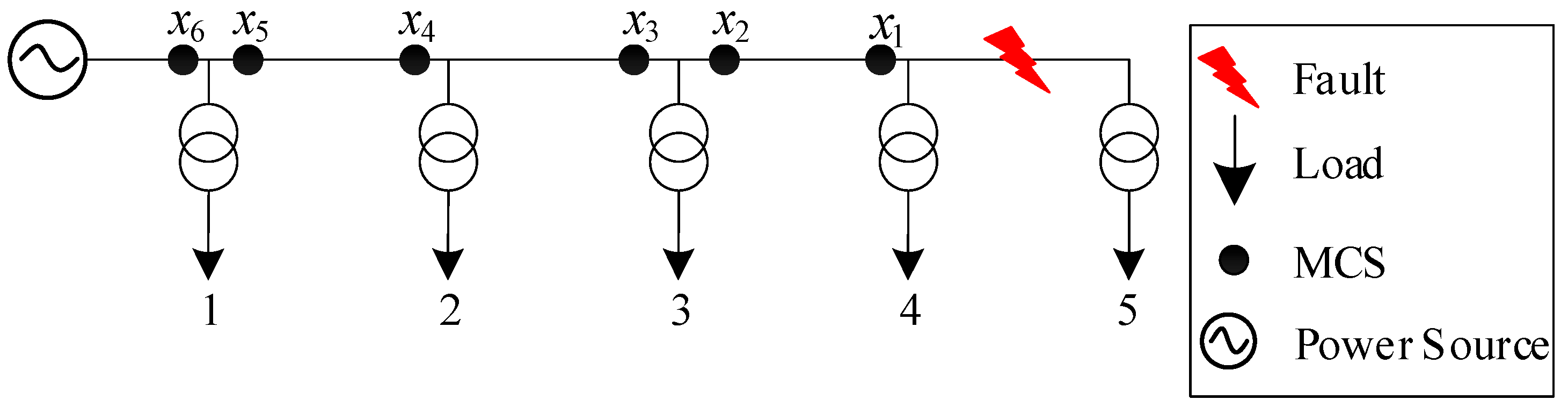
For the linearization of t_fk, it is sufficient to linearize the analytical expression of t_iso,fk. If n ≥ 2, we define auxiliary variables ${\tau }_{fk}^{(n)}=(1-x_1)(1-x_2)(1-x_3)\dots (1-x_n)$ and introduce a group of linear constraints. To illustrate this, a simple topology was designed, using the fault on line 4–5 in Figure 3 as an example:

(1)

If n = 2, the fault isolation time $t_{iso,4-5,3}(\mathit{x})$ of node 3 in Figure 3 can be expressed as $(m-r)(1-x_1)(1-x_2)+r$, thus ${\tau }_{fk}^{(2)}=(1-x_1)(1-x_2)$, and the following linear constraints are introduced:

$${\tau }_{fk}^{(2)}\le (1-x_1)$$

(22)

$${\tau }_{fk}^{(2)}\le (1-x_2)$$

(23)

$${\tau }_{fk}^{(2)}\ge (1-x_1)+(1-x_2)-1$$

(24)

(2)

If $n\ge 3$, the fault isolation time $t_{iso,4-5,2}(\mathit{x})$ of node 2 in Figure 3 can be expressed as $(m-r)(1-x_1)(1-x_2)(1-x_3)+r$, thus ${\tau }_{fk}^{\left(3\right)}={\tau }_{fk}^{\left(2\right)}(1-x_3)$; Similarly, ${\tau }_{fk}^{(n)}={\tau }_{fk}^{(n-1)}(1-x_n)$. Accordingly, the following linear constraints are introduced:

$${\tau }_{fk}^{(n)}\le {\tau }_{fk}^{(n-1)}$$

(25)

$${\tau }_{fk}^{(n)}\le (1-x_n)$$

(26)

$${\tau }_{fk}^{(n)}\ge {\tau }_{fk}^{(n-1)}+(1-x_n)-1$$

(27)

In a specific line fault scenario, by using recursion, the value of t_fk can be computed step by step:

$$t_{iso,fk}(\mathit{x})=(m-r){\tau }_{iso,fk}^{(n)}+r$$

(28)

Similarly, CDF_fk can be obtained:

$$CD{F}_{fk}(\mathit{x})=(CD{F}_{MCS}-CD{F}_{RCS}){\tau }_{iso,fk}^{(n)}+CD{F}_{RCS}$$

(29)

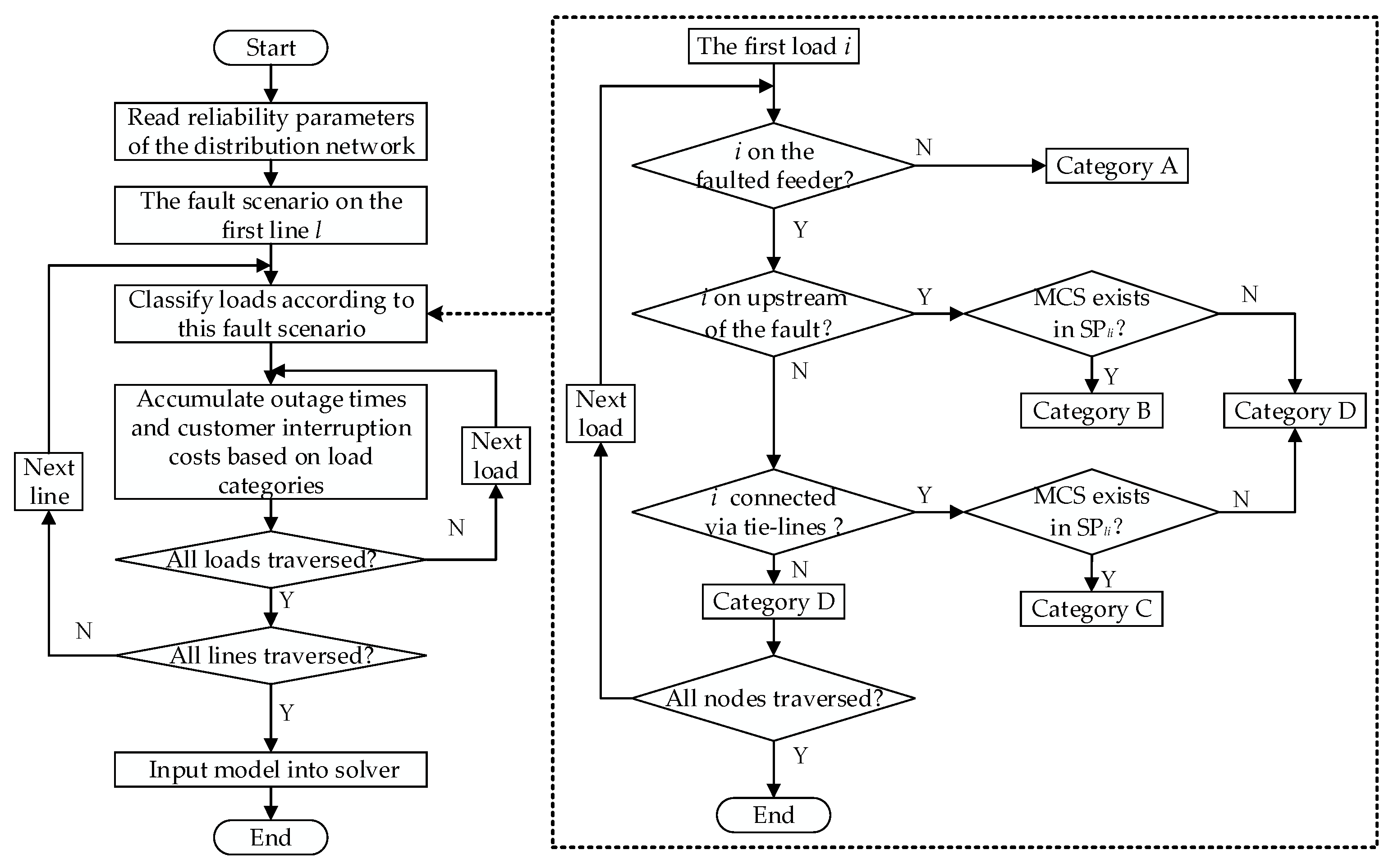
Therefore, the product of t_fk and CDF_fk in the CIC term of the objective function is replaced by Equation (16), and the corresponding constraints (17)–(20) are added to the model. Furthermore, the bilinear terms involving binary variables in t_fk or CDF_fk are linearized using Equations (22)–(27), thereby transforming the original model into a linear formulation. The detailed solution procedure is illustrated in Figure 4. Ultimately, the MILP model for optimal RCS configuration is formulated as follows:

$$\min LCC(\mathit{x})+CIC(\mathit{x})$$

(30)

$$LCC(x)=(1+h)c_{RCS}{K}_{RCS}{\displaystyle \frac{r_0{(1+r_0)}^{\tau }}{{(1+r_0)}^{\tau }-1}}$$

(31)

$$CIC(x)={\displaystyle \sum _{f\in {\Omega }_f}{\displaystyle \sum _{k\in {\Omega }_b}{\lambda }_f{P}_k^{LP}{z}_{fk}}}$$

(32)

$$s.t. \left(1\right)~(6),(16)~(20),(22)~(29)$$

(33)

In this study, we focus on distribution network scenarios with sufficient line capacities. In such cases, the large conductor cross-sections and low line resistance typically result in minimal voltage drops, and operational limits violation is unlikely to occur. Therefore, it is reasonable to neglect power flow and voltage constraints in the model formulation. It is worth noting that similar modeling assumptions and simplifications have been validated in [8,12].

4. Simulation Results

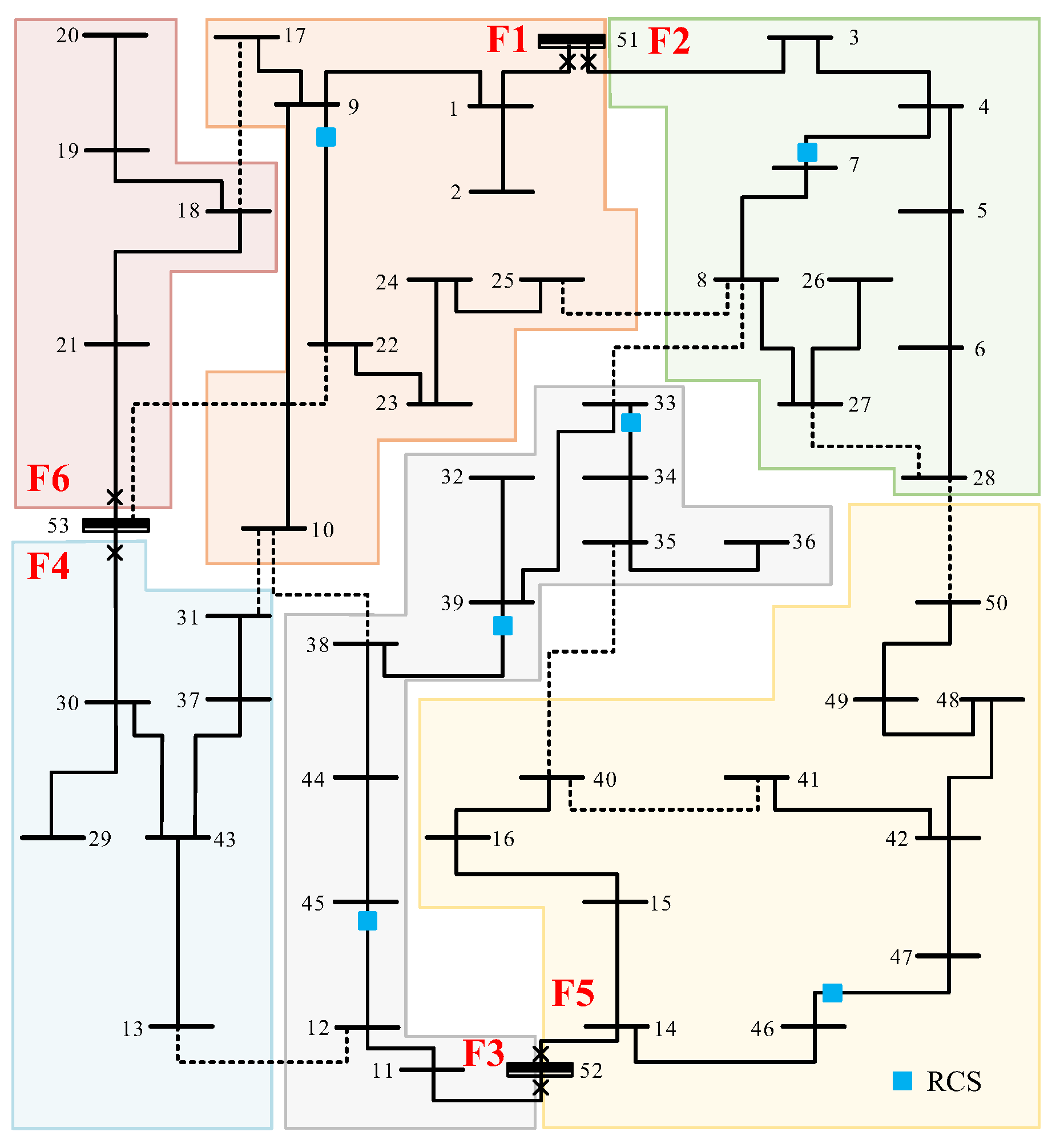
In this section, the proposed method is validated on a 53-node and a 33-bus test system. The 53-node test system consists of three substations, 50 load nodes, 50 normally closed lines, and 11 tie-lines [18]. The single-line diagram is shown in Figure 5. Under normal operating conditions, the total active and reactive power demands are 45.7 MW and 22.1 MVar, respectively. The rated capacities of the three substation nodes (nodes 51, 52, and 53) are 33.4 MVA, 30 MVA, and 22 MVA, respectively. The system operates at a voltage level of 13.8 kV, with the per-unit voltage constrained within the range of [0.95, 1.05].

It is assumed that all line segments are equipped with MCSs at both ends, except at the feeder outlets. The proposed model is implemented in MATLAB 2023a. The fault location time t_loc is set to 1.2 min. The operation times of RCS and MCS are set to 3 min and 48 min, respectively. The fault repair time t_rep is set to 4 h [19]. The unit energy interruption costs due to RCS operation, MCS operation, and fault repair are set to $0.04/kWh, $3.42/kWh, and $5.00/kWh, respectively. The failure rate of each line is set to 0.04 faults per year [20]. The unit investment cost and lifetime of each RCS are set to $20,000 and 20 years, respectively [21]. The discount rate is set to 0.1. The RCS operation and maintenance cost is assumed to be 3% of its capital investment annually. The model is solved using the Gurobi optimizer on a computer equipped with an Intel i5-13500HX processor. The stopping criteria are defined as either reaching an optimality gap of 0.01%.

4.1. Analysis of Planning Results

The proposed model is first tested under the constraint of a fixed total number of RCSs deployed in the system. This allows for evaluating the level of supply reliability that can be achieved under different RCS configuration quantities. The corresponding calculation results are illustrated in Figure 6 and Figure 7. The model achieves a single solution time of 0.6798 s, demonstrating good computational efficiency.

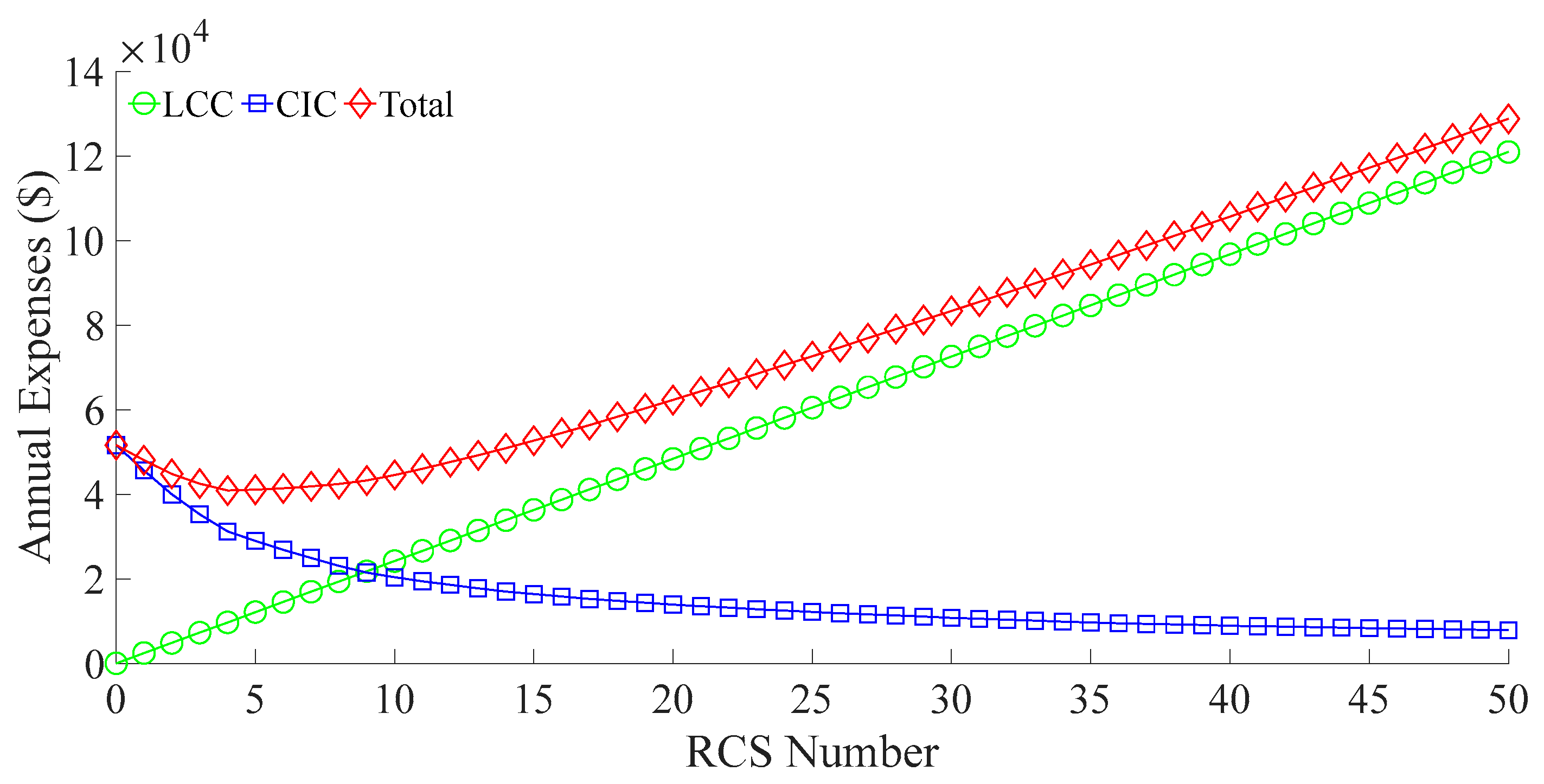
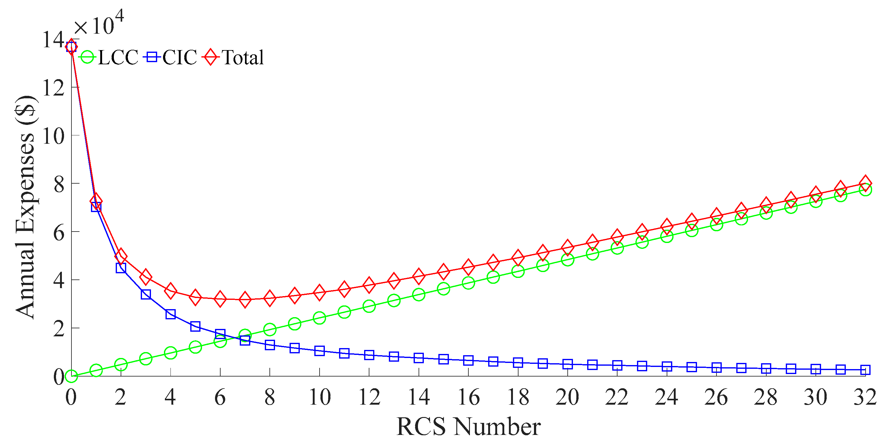
As shown in Figure 6, the CIC decreases consistently with the increase in the number of RCSs, while the LCC increases gradually. The total cost, defined as the sum of CIC and LCC, exhibits a convex trend—initially decreasing and then increasing. The minimum total cost of $40,864.3 is achieved when four RCSs are deployed. When the number of RCSs ranges from zero to four, the total cost decreases because the system’s reliability is initially low, and even a small number of RCSs can significantly improve supply restoration. In this stage, the reduction in CIC outweighs the increase in investment. However, beyond this point, although CIC continues to decline, the increase in equipment cost becomes more dominant. As a result, the total cost starts to increase approximately linearly with the number of RCSs.

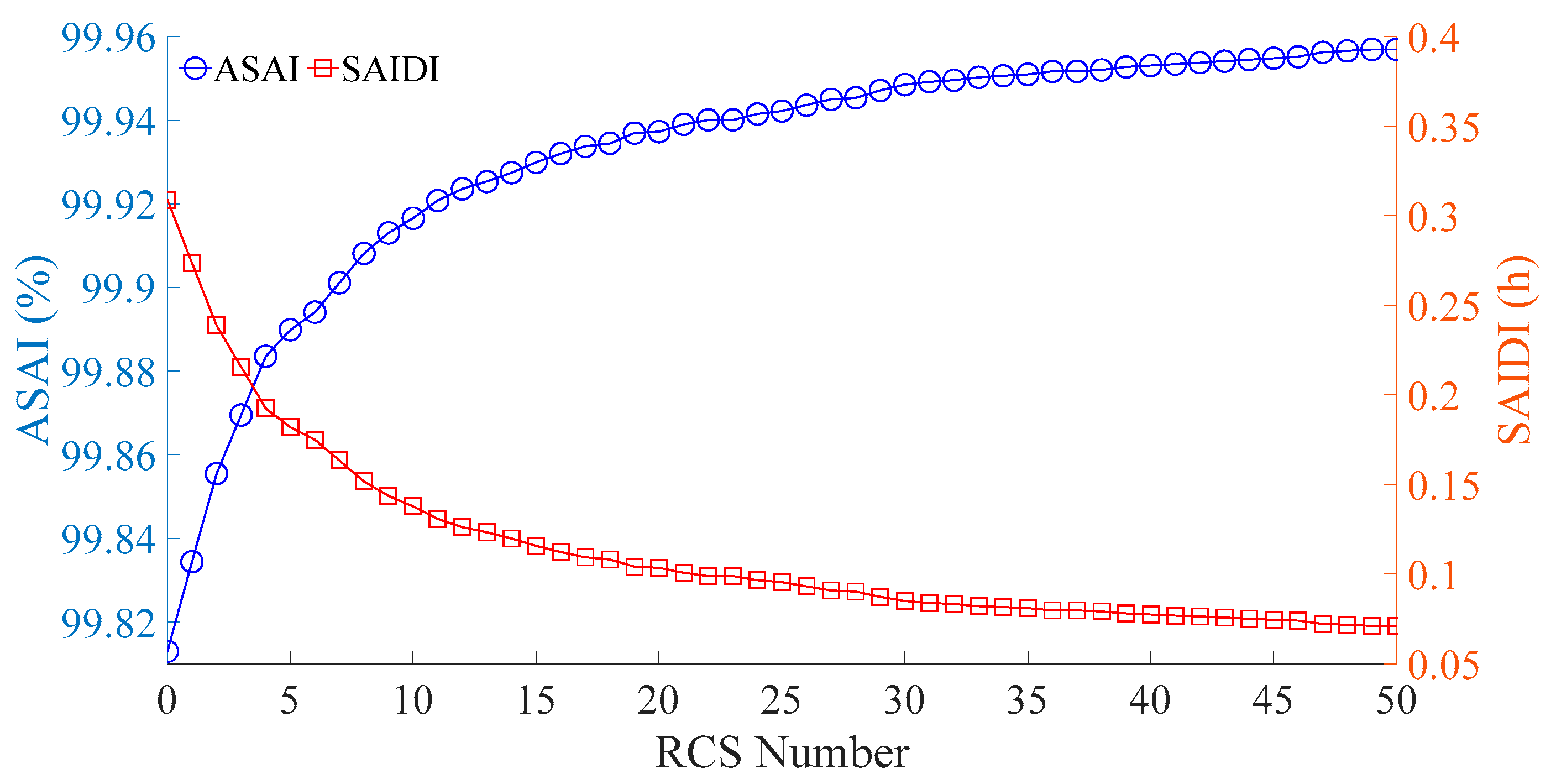
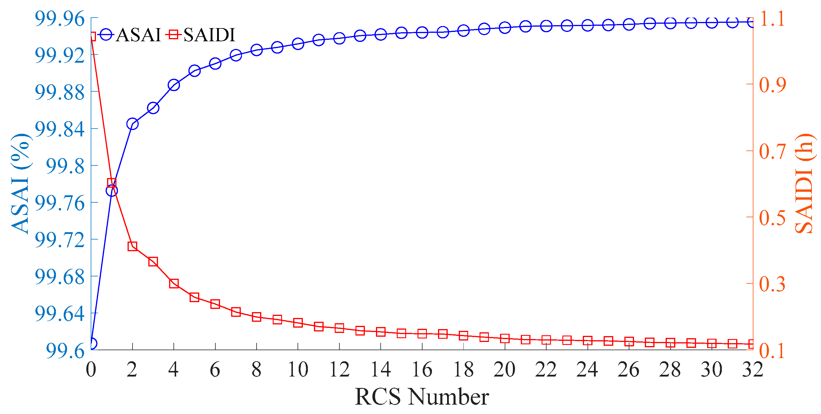
As shown in Figure 7, both ASAI and SAIDI improve with more RCS installations, though the rate of improvement slows over time. Initially, additional RCSs significantly enhance the system’s fault isolation and response capabilities, sharply reducing outage frequency and duration. However, after reaching a certain reliability level, further deployment results in only marginal gains, causing the reliability indices to approach a saturation point. Specifically, ASAI increases from 99.81% to about 99.96%, while SAIDI stabilizes near 0.07 h.

Combining Figure 6 and Figure 7, it can be concluded that deploying approximately 25 RCSs strikes a balance between economic efficiency and system reliability for the given network. The asymptotic behavior of the ASAI curve is primarily due to the nature of the objective function, which minimizes total annual cost. The cost-optimal solution does not necessarily coincide with the solution that maximizes reliability.

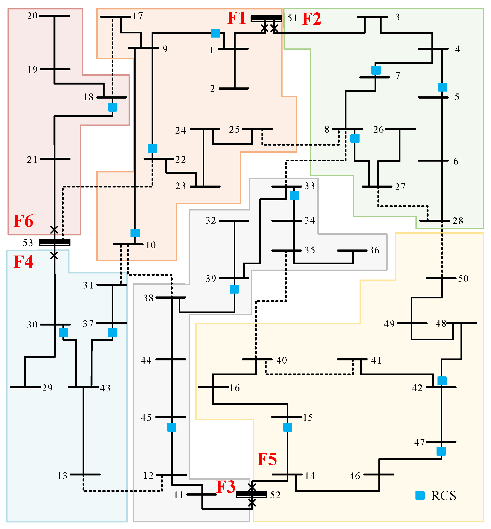
As an example, the optimal RCS allocation result under the constraint of 15 RCSs is analyzed. Figure 8 illustrates the optimal deployment configuration obtained when the total number of RCSs is limited to 15. It can be observed that when the number of available RCSs is limited, the model prioritizes placing RCSs at one end of each line to ensure basic fault isolation capability. Specifically, no RCSs are assigned to lines 23–22, 31–37, 38–44, 42–41, and 50–49. This is because, when these lines experience faults, the connected nodes can still be supplied through tie-lines. Therefore, to reduce the total annual cost, the model avoids assigning RCSs to these lines where redundancy can already be achieved via alternative paths.

4.2. Sensitivity Analysis

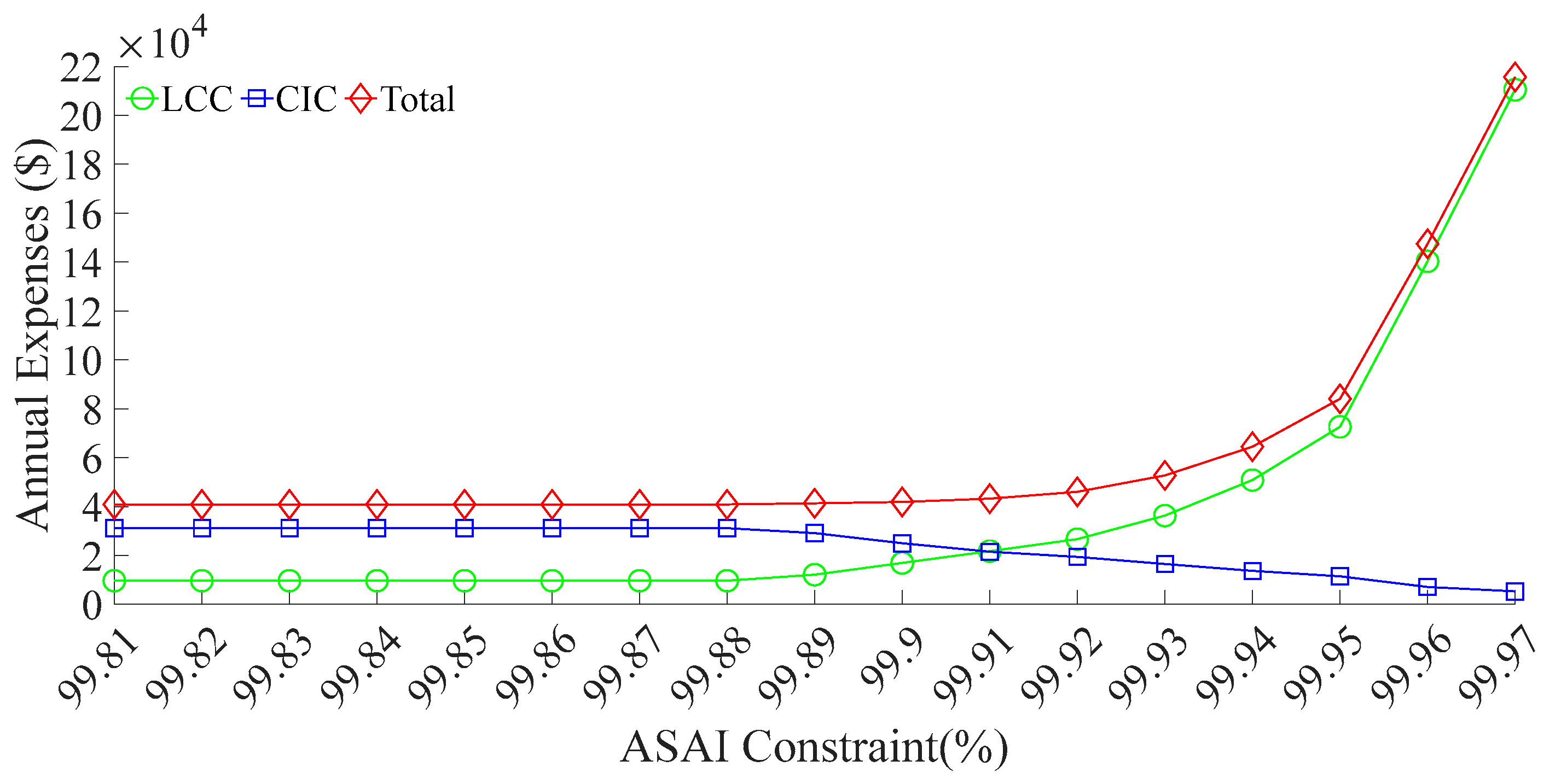
A sensitivity analysis is conducted using the ASAI as a constraint. The analysis begins by calculating the minimum and maximum achievable ASAI values for the system to assess the potential improvement in supply reliability through RCS deployment. When all switches except the circuit breakers and tie-switches are configured as MCSs, the minimum ASAI is 99.81%. Conversely, when all switches are configured as RCSs, the maximum ASAI reaches 99.97%. Based on this range, the ASAI constraint is incrementally set from 99.81% to 99.97%, with a step size of 0.01%, resulting in a total of 17 optimization runs. The corresponding results are presented in Figure 9 and Figure 10.

Based on Figure 9 and Figure 10, it can be observed that as the ASAI constraint increases, both the annual system cost and the number of deployed RCSs initially remain unchanged. This is because, under lower reliability requirements, minimizing annual cost takes precedence. In this stage, the reduction in customer interruption cost achieved by adding more RCSs is insufficient to compensate for the increased equipment investment. Therefore, deploying only a few RCSs can already raise the ASAI to a relatively high level, with four RCSs being the cost-optimal configuration. As the ASAI constraint continues to increase, the number of RCSs grows slowly at first and then accelerates rapidly. This behavior reflects the remaining potential for reliability improvement in the system. Initially, only a few RCSs are needed to meet the constraint. However, as the level of system automation improves and the ASAI approaches its upper bound, the marginal benefit of each additional RCS—measured by the reduction in average outage duration—becomes progressively smaller. To meet higher ASAI requirements, the solver begins to deploy a larger number of RCSs. When the ASAI approaches its theoretical maximum, even a small increment of 0.01% requires more than 20 additional RCSs to be installed. In this case, the annual cost becomes almost entirely dominated by RCS investment. This demonstrates the steep price required to achieve extremely high levels of reliability.

Figure 11 shows the impact of line failure rate on RCS numbers under different ASAI constraints. We set the line failure rate within the range of 0.01 to 0.05 for separate calculations [22]. It can be seen that the number of deployed RCSs increases with both the line failure rate and the tightening of the ASAI constraint. In high-failure-rate environments, more RCS devices are required to quickly isolate faults and restore power in order to meet higher ASAI targets. This indicates that increasing the number of RCSs is an effective strategy for enhancing reliability when the system is more prone to faults. At the same time, reducing the failure rate of distribution lines is also a viable and cost-effective method for improving overall system reliability. Prioritizing the installation of RCSs on lines with dense load distribution and significant fault impact can help avoid unnecessary equipment investment while achieving substantial reliability improvements.

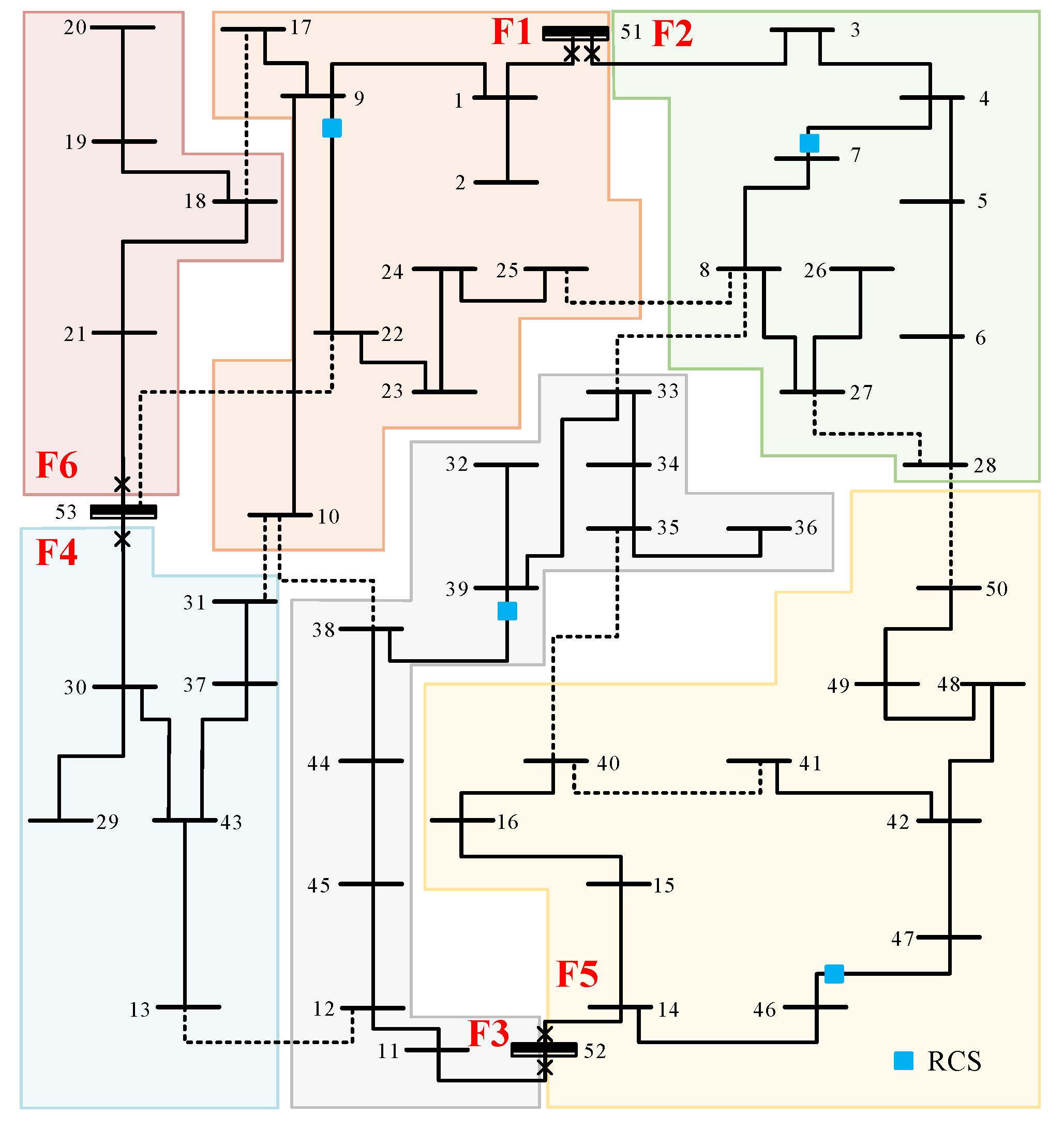
Figure 12 illustrates the optimal RCS deployment scheme when the ASAI constraint is set to 99.88%. As shown, RCSs are allocated to line 22–9 in feeder F1, line 7–4 in feeder F2, line 39–38 in feeder F3, and line 46–47 in feeder F5. Each of these feeders is equipped with one RCS. This configuration is selected because feeders F1 to F5 serve a large number of users. Allocating RCSs to these critical feeders ensures that the ASAI constraint is satisfied while maintaining cost-effectiveness. To achieve the highest reliability level of 99.97%, the model configures RCSs on all lines except tie-lines. In this scenario, RCSs are also placed at both ends of certain critical lines. This strategy ensures rapid fault isolation and power restoration, thereby satisfying strict reliability requirements at the cost of increased investment.

4.3. Robustness Test

Figure 13 illustrates the number of RCS required under varying ASAI constraints and load levels α. The results indicate that, under the same reliability constraint, higher load levels require more RCS installations to enhance system operability and supply restoration capability. However, when the ASAI constraint is below 99.93%, the number of installed RCSs remains constant. This is because the corresponding configuration yields the lowest total cost and represents the optimal solution under the given ASAI constraint. When the ASAI constraint exceeds 99.93%, the number of RCSs configured remains the same across different load levels, indicating that a certain number of RCSs must be installed to achieve high reliability.

While keeping the load levels in other areas unchanged, the load in Feeder 3 was increased to three times its original value (α = 3). The simulation results show that, in order to maintain a system reliability level of 99.88%, the required number of RCS units increased from four to six compared to the original scenario. The additional RCSs are primarily deployed on branches 12–45 and 33–44 within Feeder 3, as illustrated in Figure 14.

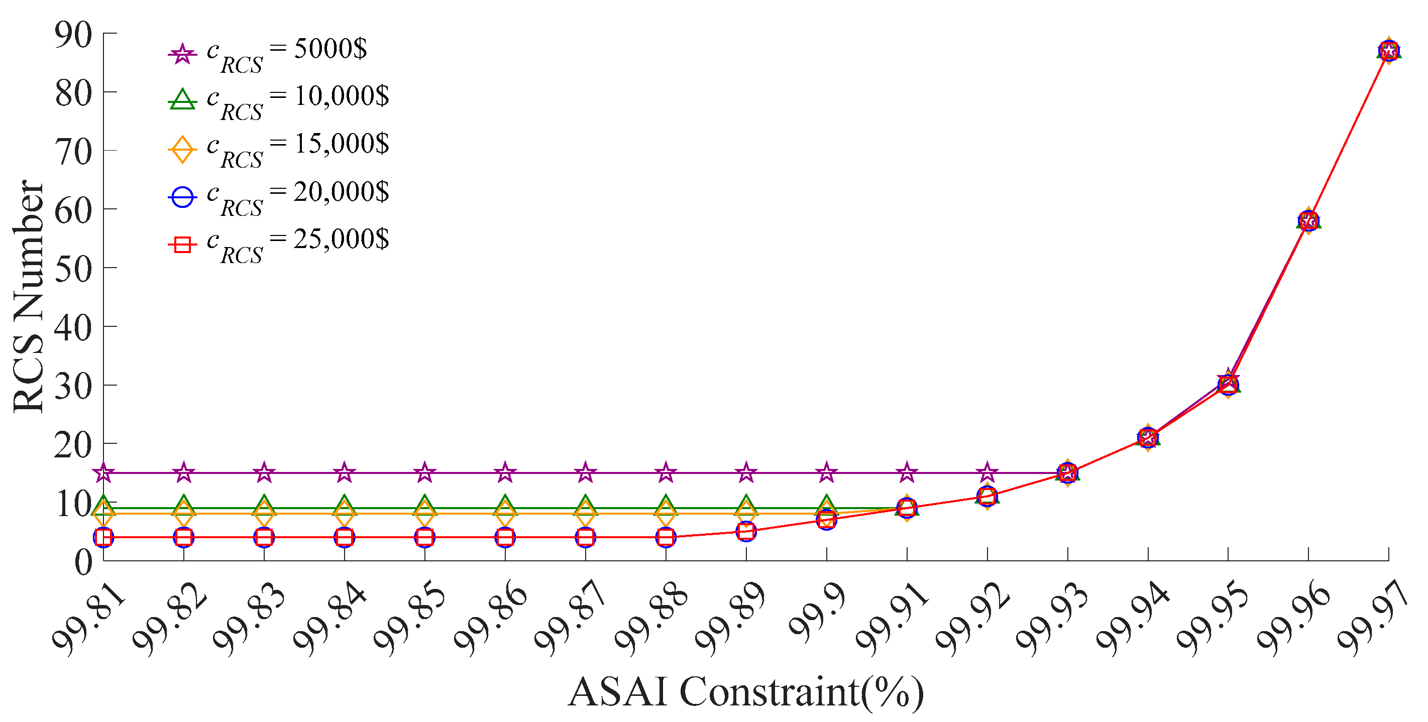
Figure 15 illustrates the number of RCSs required to satisfy various ASAI constraints under different RCS prices. The results indicate that each value of $c_{RCS}$ corresponds to a different ASAI threshold. Taking $c_{RCS}$ = 5000 $ as an example, when the ASAI constraint is below 99.93%, the number of RCSs remains fixed at 15. This is because the configuration with 15 RCSs yields the lowest total cost and thus represents the optimal solution under the given ASAI constraint. In this case, the actual ASAI value exceeds 99.93%, rendering the constraint non-binding. Increasing the number of RCSs beyond 15 results in excessive investment costs, while reducing the number leads to higher outage losses—both scenarios produce suboptimal solutions. As the ASAI constraint becomes more stringent, outage losses decrease while investment costs and total costs increase rapidly. At this point, the ASAI constraint becomes active and starts to affect the optimization outcome.

The configuration results of $c_{RCS}$ = 15,000 $ and an ASAI constraint of approximately 99.88% are presented in Figure 16.

To validate the effectiveness of the proposed model, a comparative analysis was conducted with the MINLP approach presented in [8].

Table 1. Comparison of the MILP and the MINLP method.

Constraint Type	Method	Average Solve Time	Speed-Up Factor
RCS Number	MILP	0.679 s	41.75×
	MINLP [8]	28.36 s	1× (baseline)
ASAI	MILP	1.031 s	32.61×
	MINLP [8]	33.62 s	1× (baseline)

summarizes the computational performance of both the MINLP and the proposed MILP methods under different constraint conditions. The results indicate that, while maintaining the same level of solution accuracy, the proposed MILP method significantly reduces computation time. This further confirms the correctness and practical applicability of the model.

4.4. The 33-Bus System Test

To further verify the effectiveness of the proposed model, the 33-bus test system, as shown in Figure 17, is selected for additional simulations. The corresponding results are presented in Figure 18, Figure 19, Figure 20 and Figure 21. The obtained results are consistent with those in Section 4.1 and Section 4.2 for the 53-node system, which further validates the correctness and applicability of the proposed model.

As shown in Figure 18 and Figure 19, the CIC decreases continuously as the number of installed RCSs increases, while the LCC gradually rises. The sum of these two components first decreases and then increases, yielding a minimum total cost when seven RCSs are installed. Furthermore, the system’s reliability indices improve, with ASAI increasing from 99.6% to 99.96% and SAIDI decreasing from 1.05 h to 0.12 h.

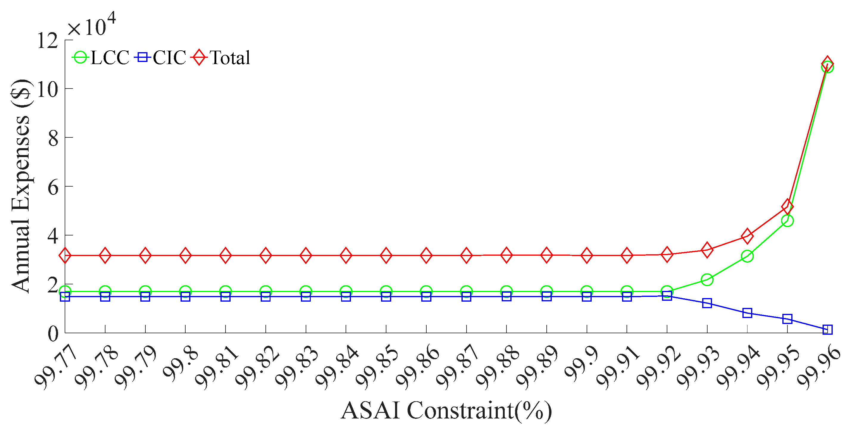
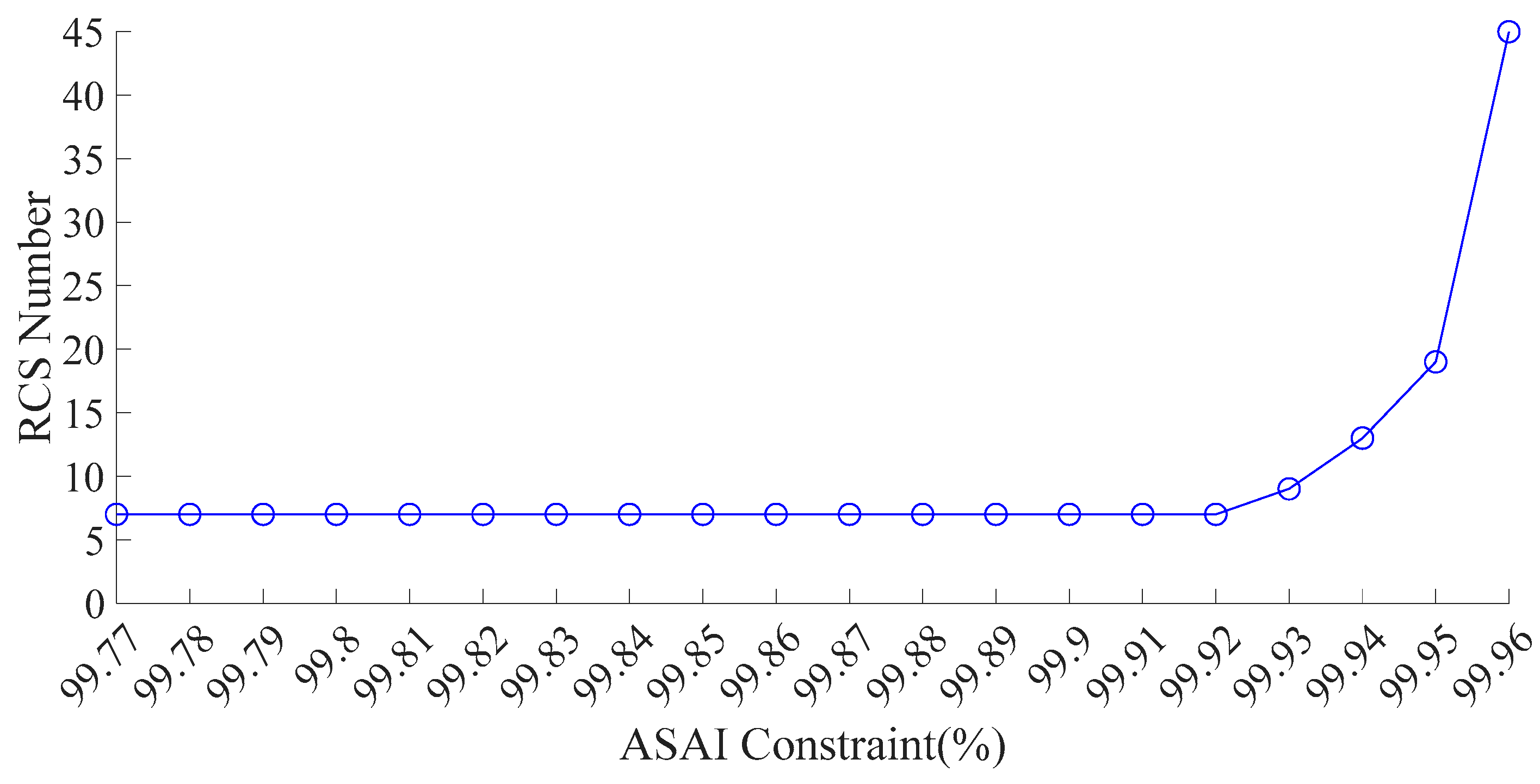
Similarly, a sensitivity analysis is conducted using ASAI as the constraint, with the ASAI constraint ranging from 99.77% to 99.96% in 0.001% increments, for a total of 20 cases. The corresponding results are shown in Figure 20 and Figure 21. The observed trends are consistent with those of the 53-node system and are, therefore, not repeated here.

Finally, we conduct a detailed comparison with Reference [16] and apply the method of [16] to the capacity-sufficient scenarios considered in this paper. In particular, considering only the impact of the number of RCSs on reliability, we tested the approaches on the 33-bus system, and the comparative results are shown in

Table 2. Comparison results of the proposed method with [16].

Method	RCS Number	Placement RCS Location	ASAI	Average Solve Time
Proposed	7	8-9U, 6-26U, 3-4D, 13-14D, 2-19D, 23-14D, 29-30D	99.919%	0.531 s
Ref. [16]	7	8-9U, 2-19U, 6-26U, 3-4D, 13-14D, 23-14D, 29-30D	99.915%	7.273 s

. “U” and “D” in the table indicate the upstream and downstream ends of a line section, respectively. It can be seen that, compared to Reference [16], the proposed method can produce better RCS allocation results within a shorter computation time.

5. Discussion

This paper proposes a MILP-based optimization model for RCS placement, aiming to minimize the total cost comprising the full lifecycle cost of RCS devices and the cost of power interruptions to users, thereby enhancing distribution network reliability. Testing with classical benchmark cases demonstrates that the model possesses strong scalability and fast computational efficiency. However, the current model employs a relatively simplified model by neglecting power flow constraints, which is the main limitation.

6. Conclusions

This paper establishes a MILP model for optimal RCS allocation under scenarios with sufficient line capacity and negligible power flow constraints. The model demonstrates strong scalability and fast solution speed. Compared to the MINLP model, the proposed approach achieves a computational speedup of approximately 30 to 40 times.

Future research should incorporate power flow constraints and multiple device constraints, such as the joint planning of RCSs, soft open points and energy storage systems, to further improve the reliability of distribution networks.