Article

Dynamic Evaluation of Forest Carbon Sink Efficiency and Its Driver Configurational Identification in China: A Sustainable Forestry Perspective

1
College of Economics and Management, Central South University of Forestry and Technology, Changsha 410004, China
2
Key Research Base of Philosophy and Social Sciences in Universities of Hunan Province “Research Center for High-Quality Development of Industrial Economy”, Changsha 410003, China
3
College of National Parks and Tourism, Central South University of Forestry and Technology, Changsha 410004, China
*
Authors to whom correspondence should be addressed.
Sustainability 2025, 17(13), 5931; https://doi.org/10.3390/su17135931
Submission received: 18 May 2025 / Revised: 22 June 2025 / Accepted: 24 June 2025 / Published: 27 June 2025

Abstract

Improving forest carbon sink efficiency (FCSE) is the key to mitigating climate change and achieving sustainable forest resource management in China. However, current research on FCSE remains predominantly focused on static perspectives and singular linear effects. Based on panel data from 30 provinces (autonomous regions and municipalities) in China from 2008 to 2022, this study integrated the super-efficiency Slack-Based Measure (SBM)-Malmquist–Luenberger (ML) model, spatial autocorrelation analysis, and dynamic fuzzy set qualitative comparative analysis (fsQCA) to reveal the spatiotemporal differentiation characteristics of FCSE and the multi-factor synergistic driving mechanism. The results showed that (1) the average value of the FCSE in China was 1.1. Technological progress (with an average technological change of 1.21) is the core growth driver, but the imbalance of technological efficiency change (EC) among regions restricts long-term sustainability. (2) The spatial distribution exhibited a U-shaped gradient pattern of “eastern—southwestern”, and the synergy effect between nature and economy is significant. (3) The dynamic fsQCA identified three sustainable improvement paths: the “precipitation–economy” collaborative type, the multi-factor co-creation type, and “precipitation–industry-driven” type; precipitation was the universal core condition. (4) Regional differences exist in path application; the eastern part depends on economic coordination, the central part is suitable for industry driving, and the western part requires multi-factor linkage. By introducing a dynamic configuration perspective, analyzing FCSE’s spatiotemporal drivers. We propose a sustainable ‘Nature–Society–Management’ interaction framework and region-specific policy strategies, offering both theoretical and practical tools for sustainable forestry policy design.

1. Introduction

As the largest carbon sink carrier in terrestrial ecosystems globally, the sustainable improvement of carbon sink efficiency (FCSE) in forests is one of the core paths to achieving the 13th and 15th United Nations Sustainable Development Goals. According to China’s Forestry and Grassland Administration, forests in China sequester over 200 million tons of carbon annually, representing 80% of the nation’s terrestrial carbon sinks. However, challenges such as unbalanced regional development, redundant resource input, and insufficient output have resulted in impediments in the sustainable improvement of FCSE [1]. With the intensification of the global climate crisis and China’s certified voluntary emission reduction (CCER) market restarting, accurately identifying the spatiotemporal driving mechanism of FCSE and developing differentiated promotion strategies has become a common concern in academic and policy circles.
FCSE is a gradual climate change mitigation method and an important approach to achieving sustainable forest resource management. Current forest efficiency research focuses on ecological efficiency [2], operational efficiency [3], production efficiency [4], carbon sink efficiency [5] and management efficiency [6]. The selection of indicators for measuring forest efficiency typically involves selecting input indicators based on the three production factors: land, capital, and labor, whereas output indicators are determined by research methods and content [7]. The land input includes forest area [8], or forest land area [9]. The capital input is the total amount of investment in fixed assets [10] or the capital stock of forestry [11]. The labor indicator is commonly measured by year-end employment in the forestry sector [12]. Output indicators include the desired output and undesired output, desired output including the carbon sequestration of forests [13], forest carbon sink efficiency [14], the gross value of forestry [15], and carbon sink value [16], and the undesired outputs are wastewater, waste gas emissions, and solid waste production [17]. The DEA [18], three-stage DEA-Malmquist [19], super-efficiency SBM [20], Stochastic Frontier Approach [21], SBM-Malmquist [22], Dagum Gini coefficient and Markov chain [23] methods have been used to measure city, province, forest region, and national forest efficiency, and analyze the characteristics of time and space. The focus of the spatiotemporal characteristics analysis is whether the FCSE has a spatial spillover effect. China’s FCSE has a positive spatial spillover effect and shows a significant spatial convergence trend [24].
The factors influencing forest carbon sink and efficiency have been classified into natural and non-natural factors [25]. The non-natural factors include two dimensions: social development [26,27] and forest management [28,29]. For natural factors, the average forest efficiency decreases after considering climatic factors [30]; however, the effects of precipitation and temperature on FCSE remain debatable. Precipitation is positively correlated with forest carbon sequestration, whereas temperature is negatively correlated with forest carbon sequestration [31]. Additionally, a study also revealed that the effects of temperature and precipitation on forest carbon sequestration are insignificant [25]. Regarding social development, carbon sink insurance, financial subsidies [32], GDP, and urbanization [33] are drivers of forest carbon sink. The primary factors influencing residents’ income distribution patterns on forest carbon sink have shifted from urbanization to urban–rural income inequality [33]. In addition, population growth, land-use policies, and technical changes are potential drivers of forest carbon sink [34]. From a management perspective, studies have been conducted to analyze the role and impact of various forest management measures on forest carbon sinks, including forest harvesting, deforestation, forest protection, and other forest management measures [35]. Several studies have comprehensively examined both natural and non-natural factors [14] and investigated the influencing factors of FCSE using Tobit [1] and the fixed effect least square (FGLS) method.
Sustainable FCSE must simultaneously fulfill three criteria: efficiency, stability, and equity. However, current studies have limitations. First, the static approaches dominate existing research. Most studies rely on cross-sectional data or traditional econometric models, which fail to capture the temporal dynamics of multi-factor interactions and overlook stability analysis. Second, owing to the lack of configurational perspective, the current analysis mainly focuses on the linear effect of a single factor while overlooking the asymmetric interaction effects of natural, socioeconomic, and forest management factors. Sustainable configurational pathways remain underexplored. These deficiencies result in homogeneous policy designs, which fail to address regional heterogeneity and ultimately undermine equitable inter-regional collaboration. The innovative aspects of this study are as follows: Firstly, the integration of the super-efficiency SBM-ML model with a dynamic fuzzy set qualitative comparative analysis (fsQCA), addressing the traditional “blind area” of QCA, spatiotemporal heterogeneity resolution multi-factor synergies. Secondly, a theoretical innovation is presented. We construct a sustainable ‘Nature–Society–Management’ interactive framework to identify region-specific sustainable pathways.

2. Methods

2.1. Super-Efficient SBM Model

The FCSE is an index used to evaluate the level of forest carbon sink in a region by considering the input of the forestry system and the output of the carbon sink. The SBM model is a DEA model that is non-radial and non-angular. It can directly handle the slack variables of input and output and avoid the defect of unreasonable input or output ratio that may exist in the radial model. The super-efficiency SBM model is developed on the basis of the combination of the SBM model and the traditional DEA model [36]. This model allows the efficiency value of the effective decision-making unit to be greater than 1 and further distinguishes the effective units. The super-efficiency SBM model takes into account the relaxation improvement of input–output, can distinguish and rank the effective decision-making units, and also avoids the proportional distortion problem of the radial model. It can flexibly handle the situations of variable return to scale (VRS) and constant return to scale (CRS), and is suitable for the complex multi-input and multi-output assessment scenarios of China’s forest carbon sink efficiency. Therefore, this paper takes the input-oriented super-efficiency SBM model as the research model [37], as shown in Formula (1)
ρ = m i n 1 1 m i = 1 m s i / x i 0 1 + 1 s 1 + s 2 ( r = 1 s 1 s r g / y r 0 g + r = 1 s 2 s r b / y r 0 b ) s .   t . x 0 = X λ + s y 0 g = Y g λ s g y 0 b = Y b λ + s b j = 1 n λ j = 1 , s 0 , s g 0 , s b 0 , λ 0
where ρ∗ is the efficiency value of DMU, n is the number of decision-making units (DMUs), m is the number of DMUS input items, x is the DMU input, 1 and s2 represent the ideal output and the unsatisfactory output, respectively, yg is the DMU desired output, yb is the DMU undesired output, s is the slack variable of DMU input, sg is the slack variable of DMU desired output, sb is the slack variable of DMU undesired output, and λ is the weight vector.

2.2. Malmquist–Luenberger Index

The essence of the Malmquist–Luenberger Index (ML) is a dynamic measurement of total factor productivity (TFP). In the “input–output” framework of forest carbon sink production, the calculation of FCSE is based on the multi-factor production function of the forestry system. Chung et al. [38] applied the directional distance function (DDF) of undesired output to the Malmquist model to obtain the Malmquist–Luenberger index and performed a dynamic efficiency evaluation that included the undesired output. It ensures that the efficiency assessment takes into account both carbon sink growth and emission reduction simultaneously. The Malmquist–Luenberger (ML) index uses the technical efficiency change (EC) and technological change (TC), as follows:
M L = E C × T C
In Formula (2), EC stands for change in technical efficiency, reflecting the changes in technical efficiency. EC > 1 indicates an improvement in technical efficiency, while EC < 1 indicates a decline in technical efficiency. TC represents technological progress and changes, reflecting the changes in technological levels. TC > 1 indicates technological progress or innovation, while TC < 1 indicates a decline in technological level. ML > 1 indicates that from the base period to the current period, the total factor productivity (TFP) has increased, that is, the carbon sink output per unit input has increased or the input per unit carbon sink has decreased. When ML > 1, it indicates that there is at least one improvement in technical efficiency or technological progress. The improvement of technical efficiency mainly lies in management optimization and the scale effect. Reduce labor redundancy to generate more carbon sinks with the same input. Reduce the cost per unit of carbon sink through intensive operation. Technological progress may involve innovations in carbon sequestration technologies and improvements in emission reduction technologies, such as planting carbon-sequestration tree species, promoting soil carbon storage technologies, and replacing diesel equipment with electric machinery. Therefore, ML > 1 indicates an increase in FCSE, and ML < 1 indicates a decrease in FCSE.

2.3. Spatial Autocorrelation Model

The spatial spillover effect is key to studying the spatial characteristics of the FCSE. The spatial autocorrelation model can effectively capture the dependence between FCSE owing to the proximity of spatial locations; that is, the observation value of one location may be affected by the observation values of its neighboring locations. Spatial autocorrelation analysis is the core content of the Geographic Information System (GIS) and spatial statistics, which can quantify the spatial dependence or spatial heterogeneity of China’s FCSE. The Global Moran’s I is the most classic and commonly used global spatial autocorrelation statistic, which is used to measure the aggregation, discreteness or randomness of spatial data within the entire study area. Therefore, the Global Moran’s I was used to investigate the spatial correlation of the FCSE, and Formula (3) is as follows:
M o r a n s I = i = 1 n j = 1 n w i j x i x ¯ x j x ¯ S 2 S 0
When I > 0, the spatial correlation is positive; when I < 0, the spatial correlation is negative; and when p > 0.05, there is significant spatial autocorrelation.
In the formula, x i is the value of the variable x i in region I, x ¯ = 1 n i = 1 n x i is the mean of the variable, s 2 = 1 n i = 1 n ( x i x ¯ ) is the variance of the variable, s 0 = i = 1 n j = 1 n w i j is the sum of all variables, w i j is the element of the spatial weight matrix w. The value range of Moran’s I is usually between [−1, 1]. I > 0, I < 0, and I ≈ 0 indicating a positive and negative correlation as well as random distribution in space. p-values beyond 0.05 indicate significant spatial autocorrelation. Otherwise, the spatial autocorrelation is not significant.

2.4. Dynamic fsQCA

FCSE is affected by numerous factors; however, limited studies have used set theory and configuration perspective to analyze it. fsQCA is a set analysis method, holding that the impact of FCSE-influencing factors on FCSE is not independent, and its significance and role depend on its combination with other influencing factors. The analysis of this configuration is achieved through set analysis. The difference between set analysis and correlation analysis techniques lies in that it analyzes sets rather than variables [39]. Therefore, after determining the results and preconditions and setting the threshold, the meas-urement variables require calibration to allow the original measurement to have an interpretable set meaning and determine the membership degree. Therefore, the fuzzy set is established, then the truth table is constructed. Calibration refers to taking into account both the category and degree differences among the cases, so that the measurement can be interpreted and meaningful [40]. Moreover, the necessary and sufficient conditions for a set analysis should be examined, comprising testing whether FCSE (Y) is a subset of a condition or combined conditions (X) (Y ≤ X), and whether a condition or combined conditions constitute an FCSE subset (X ≤ Y), respectively. However, all of this predicates that the condition configuration consistency is higher than the acceptable empirical standard (0.75). In the consistency analysis, paying attention to the case configuration frequency is also necessary, a basic requirement being that the selected case frequency should retain at least 75% of the observed cases. Finally, the configuration should be summarized and organized for analysis. Figure 1 presents the specific steps.
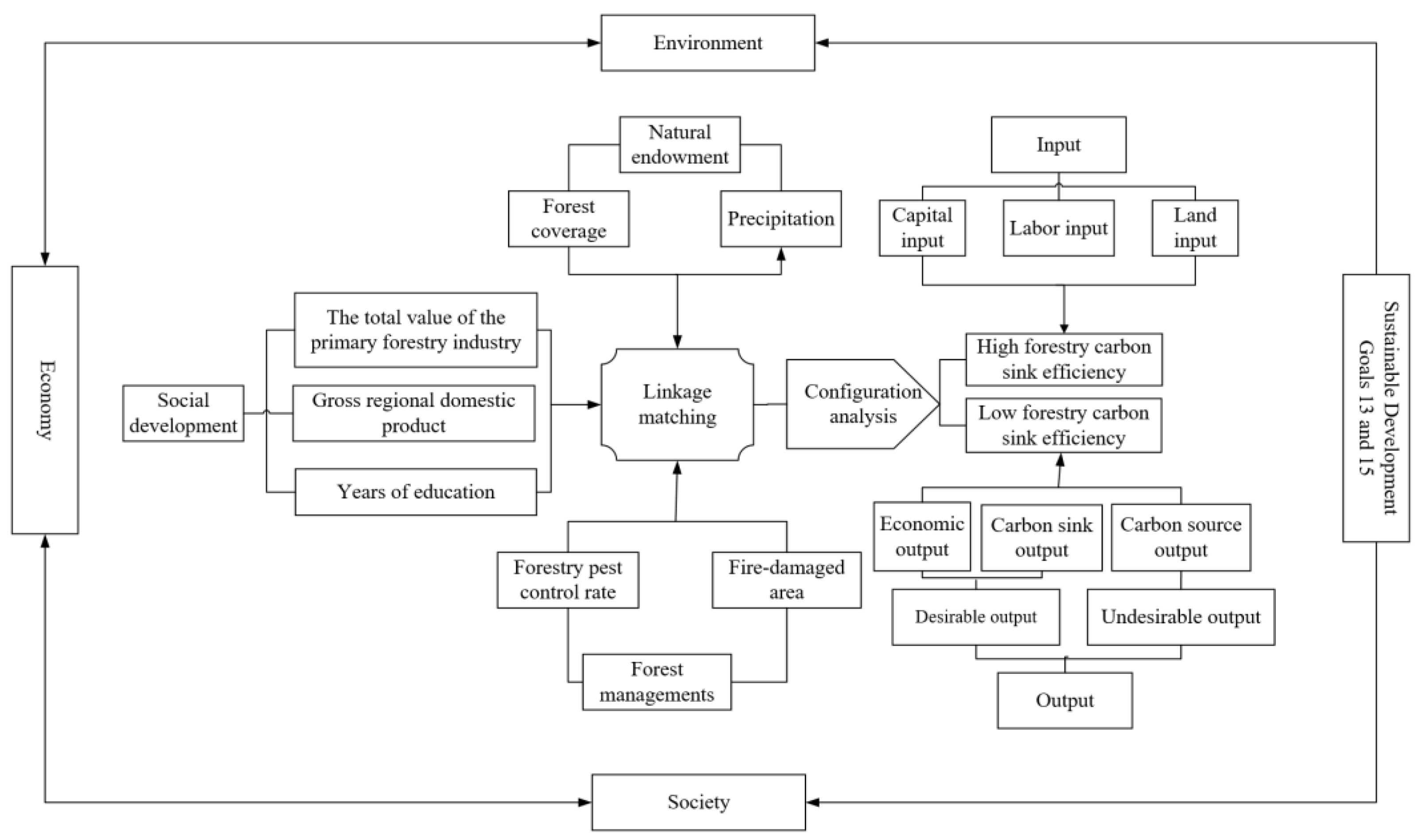
fsQCA aims to reveal the issue of causal complexity. Therefore, attention should be paid to the “time” dimension, an important source of causal complexity. However, the qualitative Comparative Analysis (QCA) method, widely used in current research, often exhibits the problem of the “time blind spot”, that is, the lack of examination of the time dimension, thereby ignoring the influence of time on a conditional configuration [41]. Dynamic fsQCA is suitable for exploring the causal relationship of “multiple concurrency” and the “joint effect” of the multi-factor interaction process on specific phenomena. Owing to the cyclical nature of tree growth and the continual improvement of FCSE, this study used the dynamic fsQCA method (Figure 2).

3. Indicators and Data

3.1. Indicator Selection

3.1.1. Evaluation Indicators Selection of FCSE

Input Indicators
In this study, the forest area of each province (autonomous region and municipality) was used to measure the land index [8], the completed investment amount of forestry fixed assets was used to measure the capital index [10], and the number of employees in the forestry system at the end of the year was used to measure the labor index [12].
Output Indicators
The forest carbon sink and the total [15] value of [13] the primary forestry industry were used as the desired output indicators, and the carbon dioxide emissions [42] generated by the energy input in the forestry production process were used as the undesired output indicators.
The forest carbon sink was calculated using an accumulation method. The accumulation method is a carbon estimation method that is based on forest stock and is an extension of the biomass method. Following the method by Zhang et al. [5], the model is expressed as follows:
C f = C b + C V + C s = V × δ × ρ × γ + α V × δ × ρ × γ + β V × δ × ρ × γ
where Cf is the total amount of forest carbon sink; Cb is the carbon sink of forest, Cv is the carbon sink of understory plants, and Cs is the carbon sink of forest land; V is the forest stock, δ is the biomass expansion coefficient, ρ is volume density, γ is the carbon content rate; and α and β are the carbon sink conversion coefficients of understory plants and forest land, respectively. Based on the definition by Xue et al. [43], α = 0.195, β = 1.244, γ = 0.500, δ = 1.900, and ρ = 0.500.
Energy is a key factor for measuring carbon dioxide emissions. Considering the availability of data and based on Lin [44] and Chen [45], this study used the emission factor method to calculate the carbon dioxide emissions from fossil energy combustion in forestry production, and the calculation formula is as follows:
C O 2 = i = 1 3 C O 2 i = i = 1 3 E i × N C V i × C E F i × C O F i × 44 12
where CO2 is the amount of carbon dioxide emissions; i = 1, 2, and 3 corresponding to the coal, oil, and gas consumed in the process of forestry production, respectively, and E is the energy consumption. NCV is the net calorific value, CEF is the carbon emission factor, and COF is the carbon oxidation factor. The carbon emission factor coefficients in this study were derived from the IPCC (2006 edition); the carbon oxidation of oil and gas was set to 1, and that of coal was set to 0.99. The selection of indicators and their descriptive statistics are shown in Table 1 and Table 2.

3.2. Influencing Factors and Theoretical Analysis of FCSE

According to current studies [46], antecedent variables were selected based on the following three aspects: natural endowment, social development, and forest management. The selection of influencing factor indicators and their descriptive statistics are shown in Table 3 and Table 4.
(1)
Natural endowment
Forest coverage (FC): Forest endowment is an important evaluation index [47] for measuring the potential of forest carbon sinks and is one of the factors affecting FCSE. The forest area and quality have considerable effects on forest carbon sinks [48]. The change in a forest area affects the total carbon storage and scale efficiency of the forest carbon sink, which, consequently, affects the overall efficiency of forest carbon sinks [1]. Forest coverage indicates the proportion of forest per unit area, and the level of forest coverage represents the number of forest plants directly involved in carbon sequestration.
Precipitation (PRE): The growth of forests is influenced by the natural environment, which is an essential factor that affects the amount of carbon sequestration in forest ecosystems. Carbon sequestration in forest plants essentially involves photosynthesis by green plants and is affected by temperature, precipitation, and other factors. Precipitation has a positive effect on FCSE, and forest carbon sequestration increases with an increase in precipitation [31]. Precipitation directly affects the humidity of combustible materials and the air, which contributes to reducing forest fires and improving forest survival rates.
(2)
Social development
The total value of the primary forestry industry (TPFI): A symbiotic relationship exists between forestry ecology and the forestry industry, and the improvement of the agglomeration level of the forestry industry promotes the improvement of ecological efficiency, specifically through externalities resulting from industrial agglomeration: the spillover of knowledge and technology, the scale effect of the industry [49], and the improvement and sharing of infrastructure. The primary role of the forestry industry is to protect and cultivate forest resources. Improving the development of the primary forestry industry contributes to protecting forest ecosystems and ensuring the stability of forest carbon sinks.
Gross regional domestic product (GDP): According to the theories of economic growth and resource dependence, the improvement of the domestic economy cannot be separated from energy consumption, which leads to an increase in carbon emissions and a reduction in carbon emission efficiency. However, economic development and ecological protection are intricately integrated, mutually beneficial, and exhibit a symbiotic relationship [50]. The level of local economic development influences the extent of investment in forestry construction, and economic growth can promote the optimization and upgrading of forestry structures and the advancement of forestry technology.
Years of education (YOS): According to the theory of planned behavior, behavioral intention is influenced by behavioral attitudes and subjective norms, which are direct factors that determine practical action, whereas people’s ecological cognition and ecological behavior are influenced by education level [51]. Farmers with high human capital levels are considerably affected by the policy of returning farmland to forests, which focuses on the ecological value and protection of forest resources [52]. The expansion of afforested areas and the sustainable management of forests are inseparable from labor force input. Education levels directly affect an individual’s knowledge and skill levels.
(3)
Forest management
Forestry pest control rate (FPCR): Insect pests change the community structure of forests, weaken forest growth, affect the absorption of water and nutrients, reduce the survival rate of forests, and lead to a decline in forest quality. Forestry pests are destructive to forest environments. Increasing the prevention and control rates of forestry pests can effectively prevent them from affecting ecological stability and reduce the output of forest carbon sinks [53].
Fire-damaged area (FDA): Frequent or large-scale forest fires can have detrimental effects on biodiversity, contributing to soil erosion and degradation, interfering with the ecological balance, releasing substantial amounts of CO2, and destroying the carbon sink function of forests. Forest fires can cause local temperature increases, resulting in forest growth retardation, and high-intensity fires may turn forest land into grassland or wasteland, causing irreversible damage to forest resources and negatively impacting FCSE.

3.3. Data Sources

We selected 30 provinces (autonomous regions and municipalities) in China from 2008 to 2022 as our research sample. The research data were obtained from the China Forestry Statistical Yearbook (http://202.99.63.178/c/www/tjnj.jhtml, accessed on 17 May 2025), China Statistical Yearbook (https://www.stats.gov.cn/sj/ndsj/, accessed on 17 May 2025), and China Energy Statistical Yearbook (https://www.macrodatas.cn/article/1147472331, accessed on 17 May 2025). Tibet was not included in the study area because of a lack of data from the Tibet Autonomous Region.
This study showed that economic development may be an important factor affecting forest carbon sinks [34]. In this study, 30 provinces (autonomous regions and municipalities) were divided into the eastern coastal region, the central inland region, and western remote region and analyzed.

3.4. Data Calibration

In this study, the entire membership, cross, and complete membership points were set to 75%, 50%, and 25% of the original data, respectively [54]. The calibration results are presented in Table 5.

4. Results

4.1. Efficiency Evaluation for Forest Carbon Sinks in China

4.1.1. Analysis of Forest Carbon Sink Efficiency in China

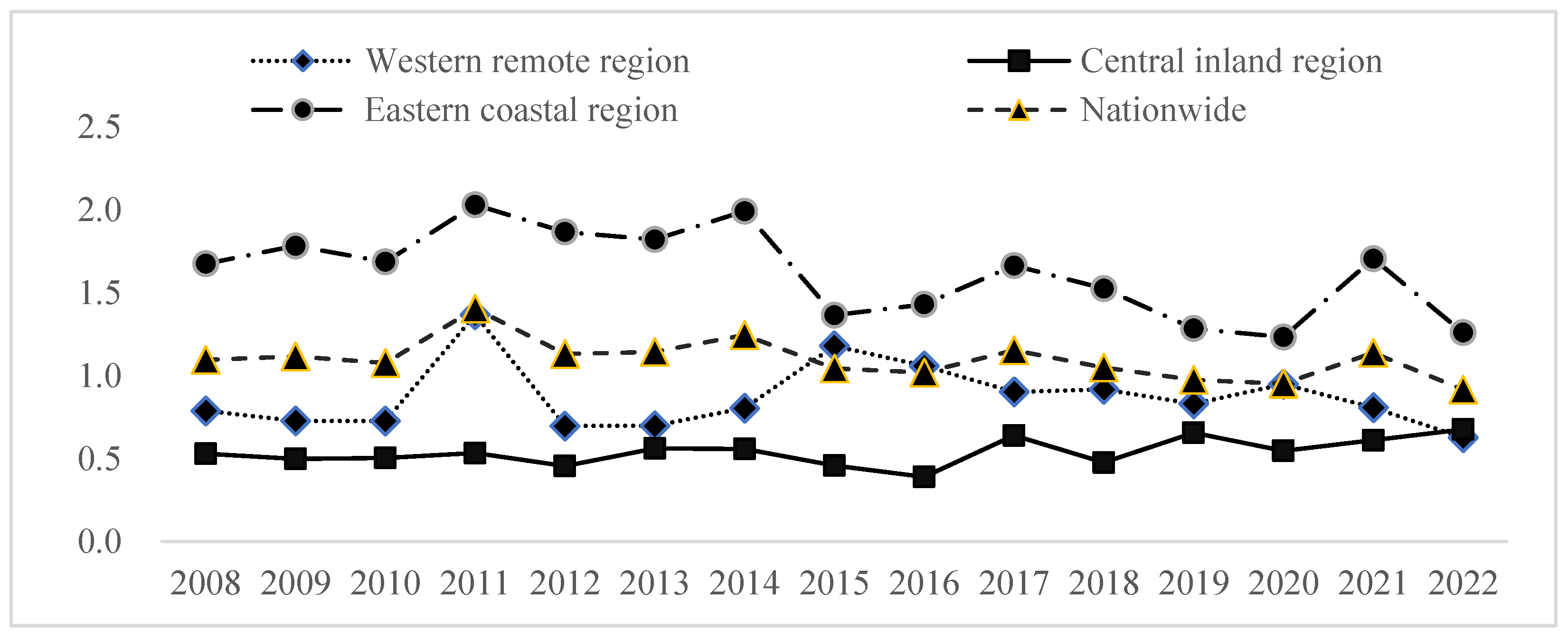
Formula (1) quantifies the FCSE through an environmentally extended productivity ratio that maximizes desirable outputs while minimizing undesirable outputs relative to resource inputs, as schematically represented in Figure 3. Figure 3 shows the time-series evolution of the FCSE. Overall, the national FCSE is basically greater than 1, showing the characteristics of “high and stable”, but regional differences are significant. During 2010–2011, the western remote region’s FCSE exhibited an upward trend, leading to an improvement in the national FCSE. This may be because China started a pilot reform of state-owned forest farms and state-owned forest areas and strengthened the cultivation of forest resources. State-owned forest areas are primarily located in the remote western region. After 2011, the FCSE in the western region experienced a brief decline, then gradually rebounded. Subsequently, it fluctuated within the normal range as the reform of state-owned forest farms and areas was still in the exploratory stage, with multiple superimposed problems such as the absence of systems, insufficient management capabilities, and limited experience. With the further reform work development, such problems have been improved, thereby driving FCSE recovery in the western region. The FCSE in the eastern coastal area is significantly higher than that in the central inland and western remote areas. A high level of economic development could bring about internal factor optimization such as forestry structure and external factors such as forestry technology, conducive to FCSE improvement. However, the central inland area is restricted by multiple natural geographical environments such as precipitation, temperature, soil, and altitude. The carbon sink function of forests remains limited.
In terms of regions, the FCSE of other provinces (autonomous regions and municipalities) showed a steadily increasing trend, except for Tianjin and Hainan (Figure 4). Under extreme high-temperature stress, the photosynthetic activity of vegetation is reduced or even stagnant, and respiration is increased. The increase in respiration exceeds the reduction in vegetation productivity, thereby aggravating the decline in the ecosystem’s carbon sink function [55]. Climate warming increases the risk of forest diseases, pests, and fires, which is a notable stress factor for the carbon sink function of forest ecosystems and significantly weakens the capacity of forest carbon sinks [56]. The Tianjin explosion accident in 2015 resulted in local climate warming as well as the direct reduction of forest resources. Owing to the growth cycle of trees, it is challenging for Tianjin to act as a maximum carbon sink in a short period. Hainan, an ecological province, is the experimental field of national tourism reform, and the overall carbon sequestration capacity of forest ecosystems has been enhanced through three measures: afforestation of Treasure Island, the establishment of scientific and technological support for forest carbon sinks, and carbon sink trading. The increase in the afforestation area is a direct factor in improving the FCSE of Hainan.

4.1.2. Spatial Variation Characteristics of Forest Carbon Sink Efficiency

The spatial distribution of FCSE is shown in Figure 5. The high-efficiency areas were mainly concentrated in the eastern coastal and southwest areas, and the low-efficiency areas were mainly concentrated in the central inland areas. The FCSE presented a Ushaped gradient pattern, with high levels from east to southwest (excluding Tibet). The southwest forest area is supported by natural endowments for high FCSE, but economic backwardness restricts long-term resilience. The Southwest forest area located in the remote western region is a major forest resource in China. Its forest area, density, and quality are all higher than those in the central inland area. The eastern coastal region has a typical forest resource endowment, but a positive two-way interaction exists between forest carbon sink and economic growth. The socioeconomic development level is an important reason for the high FCSE of the eastern coastal region [57]. In the east, economic levels and technological progress have compensated for the insufficiency of natural endowments. In the middle, due to fluctuations in precipitation and weak industries, efficiency has stagnated, forming an efficiency depression. Cross-regional ecological compensation is needed to break the lock-in effect.
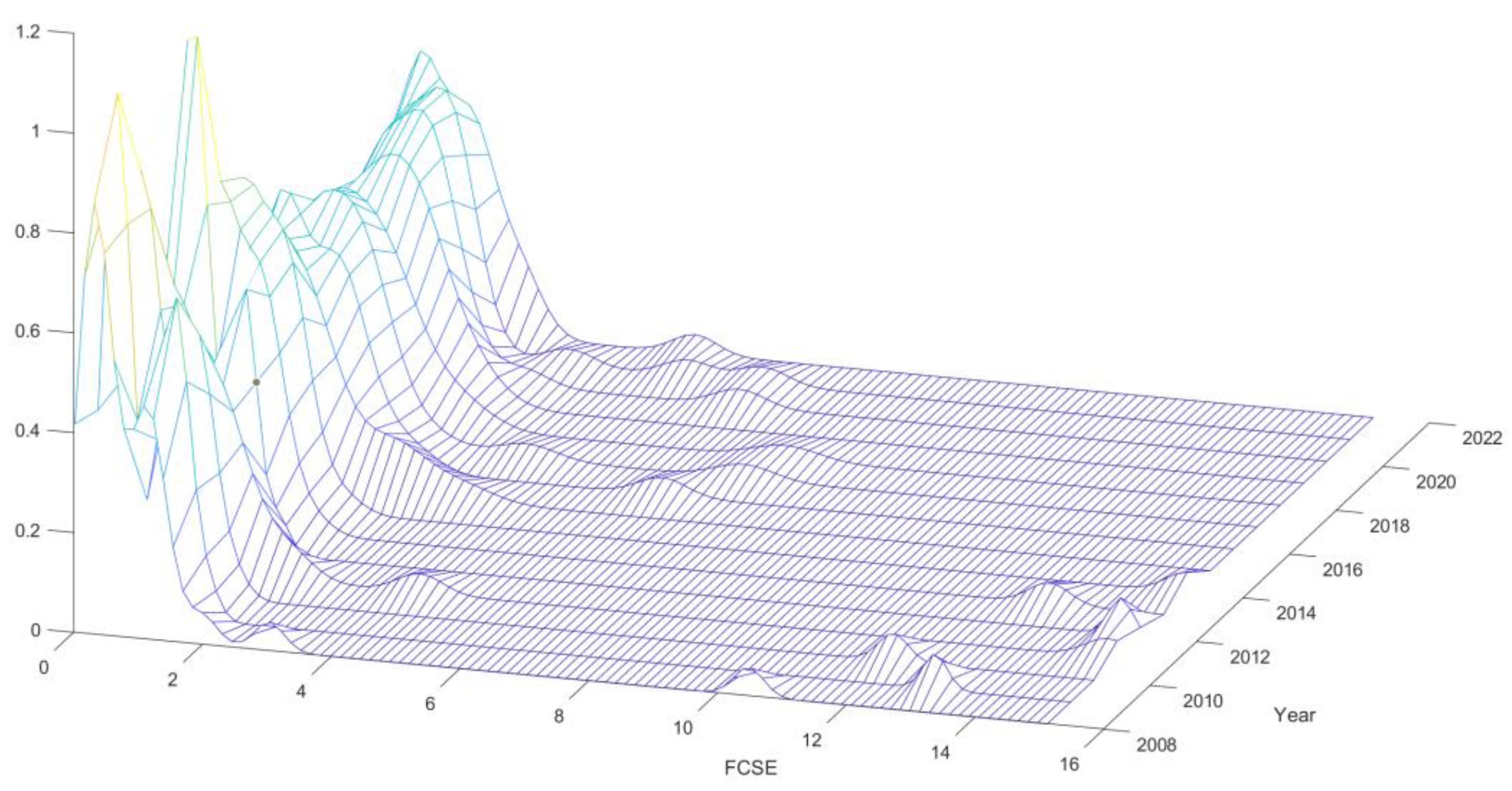
As shown in Figure 6, the trend of the kernel density curve moving to the right over time was not evident, indicating that the FCSE was relatively stable, which is consistent with the previous analysis. From the distribution pattern, the right tail was elongated, the right tail was reduced annually, and the spatial gap of the FCSE was gradually reduced. The multiple peaks changed to a single peak, and the polarization of the FCSE weakened. Inter-regional differences were the primary factors causing regional differences in forest carbon sinks in China [58].

4.1.3. Decomposition of Forest Carbon Sink Efficiency Factors

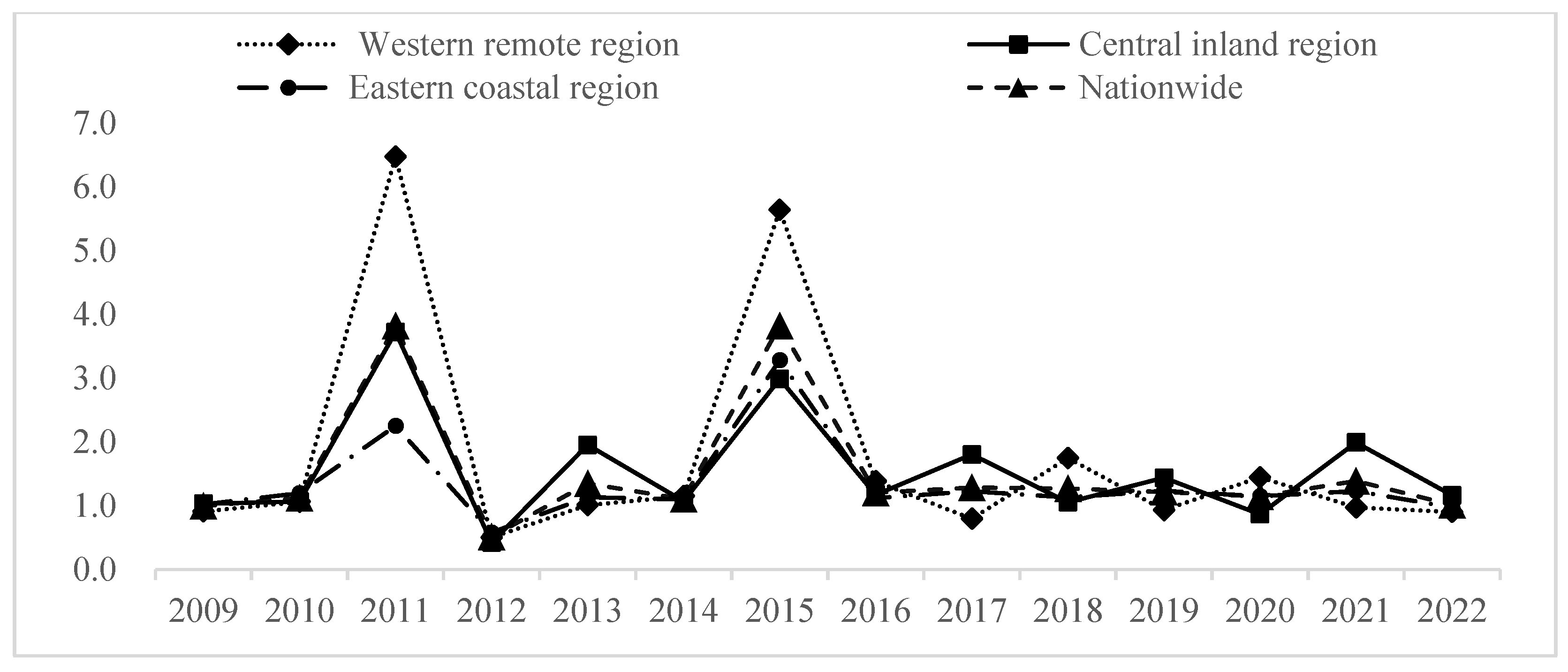
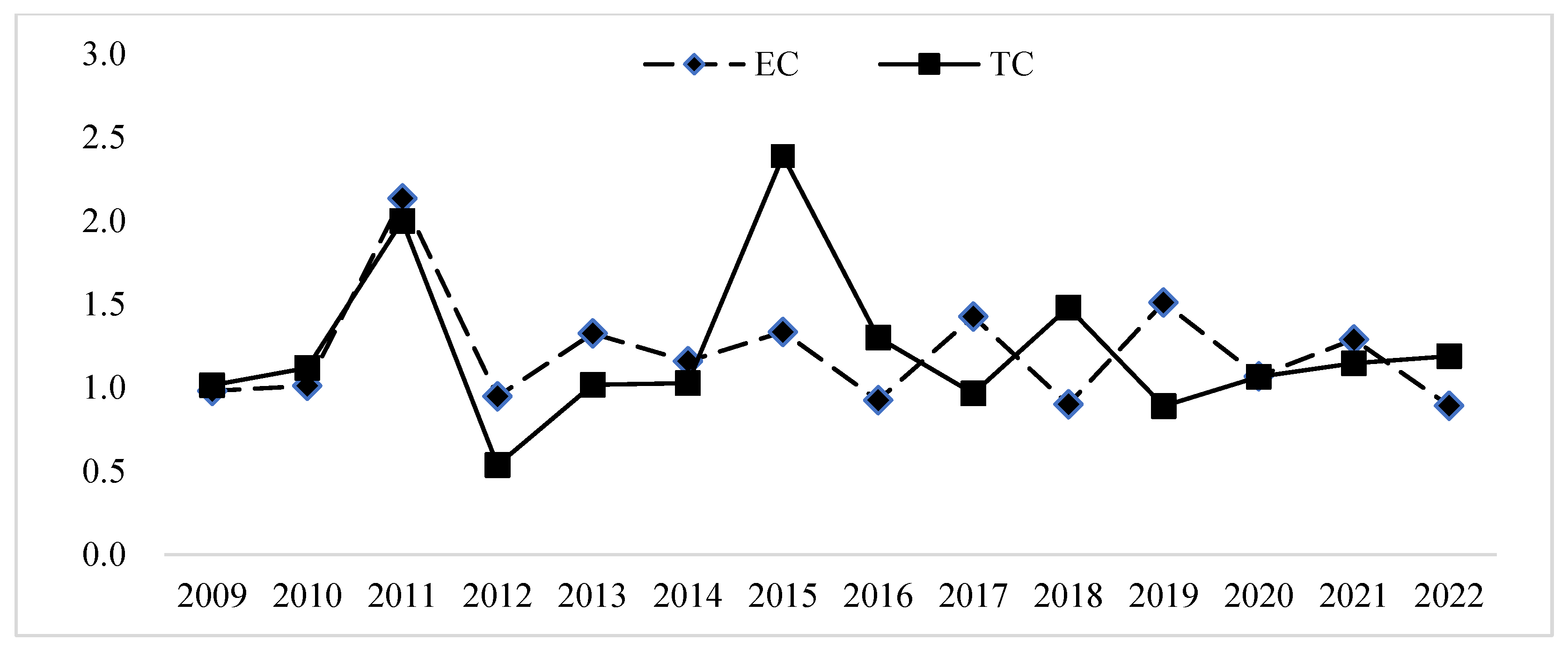
Formula (2) calculates the FCSE change index, with the results presented in Figure 7. Figure 7 shows that the change index of forest carbon sink efficiency was ˃1, indicating that the FCSE showed an overall growth trend. Except for 2011 and 2015, the trends in each region were relatively stable. The years 2011 and 2015 were in the policy-sensitive period after the end of the 11th Five-Year Plan and the imminent completion of the 12th Five-Year Plan. This indicates that institutional intervention can rapidly improve low-efficiency areas, but long-term capacity building needs to be accompanied. For further analysis, the Malmquist–Luenberger (ML) was decomposed into the efficiency change (EC) and technical change (TC), as shown in Figure 8 and Table 6. The mean value of the ML index was 1.04, the mean value of EC was 0.9, and the mean value of TC was 1.21. Technological progress leads to the improvement of FCSE, with TC being the main growth driver. However, EC has remained sluggish for a long time, reflecting the unsustainability of extensive management. The mean value of EC was lower than that of TC, indicating that technical efficiency was the main factor limiting the development of FCSE. The input–output efficiency of technology was not optimal, and there was technological progress or innovation. With the advancement of policy support and technological progress, the carbon sink potential of China’s urban agglomerations has continuously improved, and low-level areas have gradually decreased [59].

4.1.4. Spatial Autocorrelation Test of Forest Carbon Sink Efficiency

Formula (3) tests the spatial autocorrelation of China’s FCSE, with the results presented in Table 7. Table 7 indicates that most of Moran’s I index values for FCSE were negative, and from 2017 onwards, the index shifted to positive, indicating a transition from a negative to a positive correlation. No significant spatial autocorrelation was observed in FCSE, exhibiting discrete spatial patterns. This may be because both the carbon sink and carbon source influence the FCSE, and the connectivity direction or spillover size of the carbon sink and carbon source are inconsistent.

4.2. Analysis of Driving Factors of China’s Forest Carbon Sink Efficiency

4.2.1. Necessity Analysis

A variable is a necessary condition for the outcome variable when consistency is ˃0.9 and coverage is ˃0.5 [60]. In the fsQCA panel data analysis, the between consistency adjusted distance was ˃0.2, indicating a time effect. The within consistency adjusted distance was ˃0.2, indicating an individual effect. When the adjustment distance was ˂0.2, the accuracy of the summary consistency was high, and the support for the decision result was substantial [61]. The results are presented in Table 8. The consistency coefficients of all the variables were ˂0.9; therefore, there were no necessary conditions for these factors.
Further analysis of causal combinations with between consistency adjusted distance ˃ 0.2 was performed, as shown in the attached Table A1. The results showed that from 2008 to 2009, the consistency level between the Case 4 and Case 8 groups was 0.9%, with a coverage rate of 0.5; however, all failed the necessary condition test by the X-Y scatter plot test, as shown in Figure 9 [62].

4.2.2. Configuration Analysis

The core of the fsQCA method is the configuration analysis of the different antecedent conditions that affect the outcome variables. Because the threshold of case frequency should be at least 75% of the total number of cases, combined with the actual research situation [63,64,65], this study set the case frequency at four. The original consistency threshold was set to 0.8 [60]. To maintain the reliability of the results, we excluded data with a PRI consistency below 0.6 [66]. Because no necessary conditions of the study existed, all directions of the desired variables were set to “-,” indicating uncertainty.

4.2.3. Pooled Results

The overall consistency of the configuration was 0.822, and the consistencies of the three configurations were 0.824, 0.828, and 0.753, which were all greater than the standard value of 0.75 (Table 9). Therefore, the results had a strong explanatory power and were a sufficient condition for high FCSE. The between consistency adjusted distance was ˂0.2, and the within consistency adjusted distance was ˃0.2, indicating that there was no significant time effect of the variable, but a significant individual effect was present. The intermediate and simple solutions were all summed with no auxiliary conditions. The specific analysis is as follows.
Configuration 1: “Precipitation–economy” synergy: This path explained 17.5% of the high-level FCSE cases, of which 7.8% of the provinces could only be explained by this path. This path highlights abundant precipitation and a developed socioeconomic status. Despite the low output value of the primary forestry industry in the target region, improving water conditions and developing economies can still effectively improve the FCSE. A positive relationship was observed between precipitation, economic growth, and FCSE [34,57]. Therefore, under the condition that ensures humidity of the forest growth environment, the rapid development of the social economy can effectively improve FCSE.
Configuration 2: Multi-factor co-creation: This pathway explained 17.9% of the high-level FCSE cases, and 10.2% of the provinces could only be explained by this pathway. The configuration showed that FC, TPFI, and GDP were missing and were jointly affected by PRE, YOE, FPCR, and FDA. The absence of TPFI and GDP conditions indicated that the configuration was mainly affected by natural endowments and forest management.
Configuration 3: “Precipitation–industry-driven”: This path explained 9.1% of the high-level FCSE cases. This path showed that in areas with abundant precipitation and a high output value of the primary forestry industry, forest growth recovery and improvements in FCSE could be achieved through natural precipitation and industrial cultivation practices despite low forest coverage and large areas affected by forest fires. Forestry economic development and ecological protection are comprehensively integrated and mutually promote each other, which is consistent with the results of previous studies [50]. Therefore, under sufficient precipitation, the rapid development of the primary forestry industry can effectively improve FCSE.
A horizontal comparison indicated that precipitation is the core condition in all configurations and notably affects the FCSE, which is consistent with other studies that suggest that precipitation has a positive effect on the FCSE [41,58]. Among natural endowments, forest coverage is an important indicator for measuring the richness of forest resources, while the annual average precipitation is positively correlated with forest land quality [67], which indicates that forest quality plays a more critical role in FCSE than in forest areas. Ensuring the moisture required for forest growth and maintaining the moisture of the forest ecosystem is necessary to improve the FCSE. FC, GDP, YOE, FPCR, and FDA had no effect in some configurations but were critical in others, indicating that their effects on FCSE varied depending on their combination with other factors. In the three configurations, the TPFI exhibited the status of missing, no effect, and core, indicating that its influence on the development of FCSE differed with different combinations of factors. The antecedent variables in the configuration were all core conditions, and there was no complementary or substitution effect; therefore, any element in the configuration could not be ignored.

4.2.4. Between Result

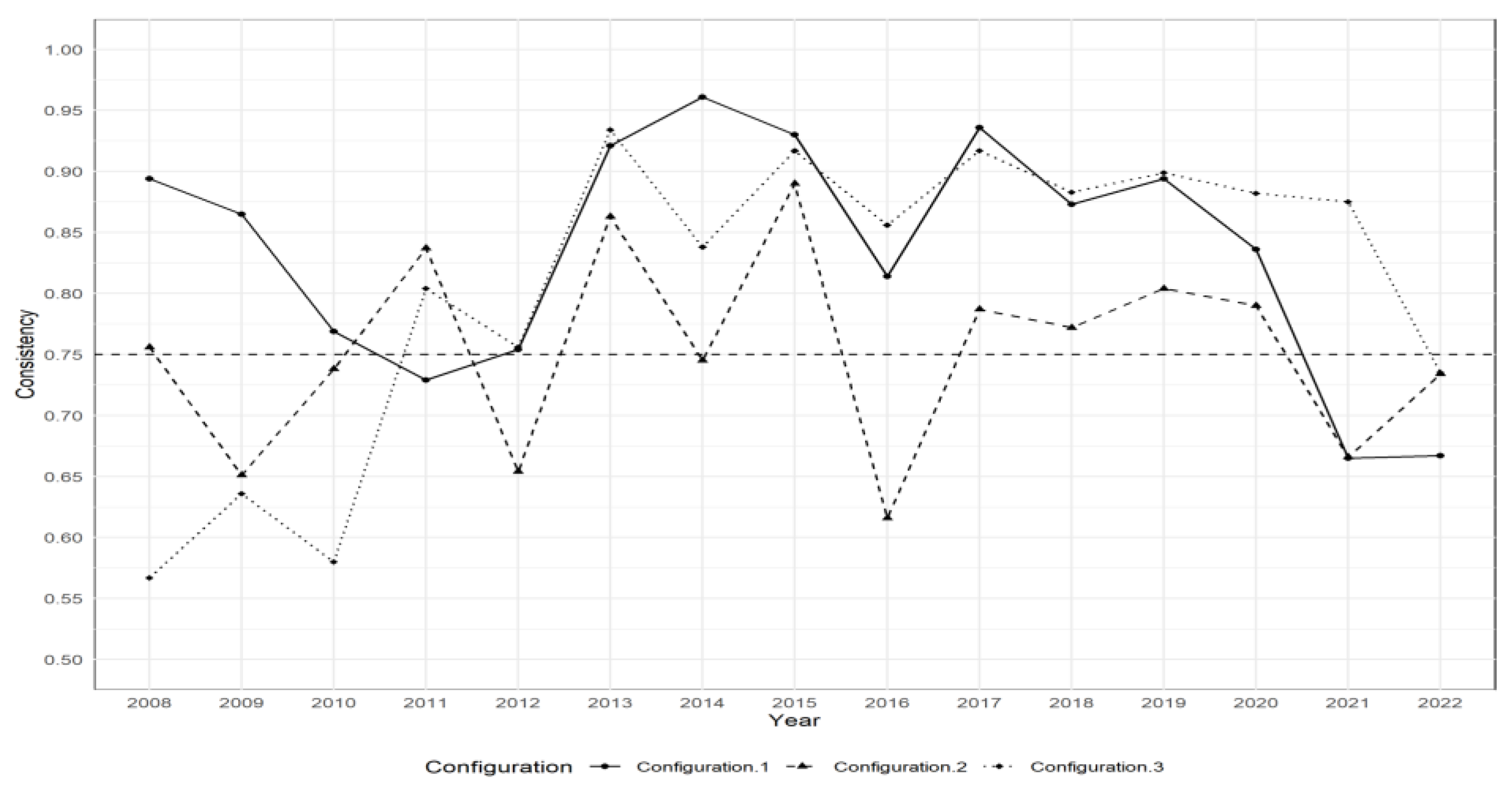
Traditional QCA has a time-blind zone; therefore, dynamic QCA was used to analyze the between consistency to explore the time effect of the configuration. According to Table 9, the between consistency adjusted distance of the three configurations was ˂0.2, indicating no significant effect of time on these configurations.
As shown in Figure 10, the between consistency of Configuration 1 was basically higher than 0.75, and the variation trend of consistency between Configurations 2 and 3 was approximately similar, but the consistency varied considerably, and the consistency between some groups was ˂0.75. Further observations showed that the between consistency below 0.75 was mainly concentrated during 2008–2010 and 2020–2022, and the between consistency of Configuration 2 was also lower than that of the standard value in 2012 and 2016. The specific reasons may include the following: First, the financial crisis began in 2008. Although the government has implemented various measures, restoring stability continues to require time. The impact of the financial crisis did not gradually weaken until approximately 2010. Second, from 2020 to 2022, the country experienced the severe impact of the epidemic and continuous adjustment of prevention and control measures, and the market environment was depressed, which affected social development. Third, the State of Climate 2012 report indicated that 2012 ranked among the ten hottest years on Earth, and excessive temperatures caused substantial water evaporation, which affected the survival of trees. Fourth, the reform of state-owned forest farms in 2015 remained in the exploratory stage in 2016, with challenges such as limited employment mechanisms, difficulties in employee management, and a lack of subsidies. However, this phenomenon did not affect the overall interpretative strength of the configuration, which remains a reference value for normal FCSE measurements.

4.2.5. Within Results

The within consistency adjusted distance for all configurations was ˃0.2, indicating that the explanatory power of each configuration differed significantly across provinces. In most provinces, at least one configuration had a strong consistency, but not all the configurations were applicable to individual provinces, such as Shanxi, Shaanxi, Liaoning, and Inner Mongolia, probably because most of the configurations were located in the Midwest, where the economy is relatively underdeveloped, natural endowments are limited, and forestry economy development conditions are lacking. By analyzing the effectiveness of each configuration case, we found that Configuration 1 covered Shanghai, Jiangsu, Guangdong, and Henan; Configuration 2 included Yunnan, Fujian, Zhejiang, Guizhou, and Guangxi; and Configuration 3 was distributed in Sichuan, Hubei, and Anhui. Most high-level cases were concentrated in economically developed areas, and the differential distribution of cases indicated the unbalanced development of FCSE in China.
The mean value of regional coverage presented in Table 10 indicates that the case coverage areas explained by Configuration 1 were predominantly located in the eastern and central inland regions. Owing to the limitations of social and economic conditions, the level of adaptation of the western remote region to Configuration 1 was not high. Configuration 2 showed no significant difference in the explanatory case coverage across the eastern, middle, and western remote regions, possibly owing to universal application beyond the economic development level. The cases explained by Configuration 3 were mainly distributed in the central inland region. This type of configuration is suitable mainly for areas with low forest coverage and a focus on forestry development.

4.2.6. Robustness Test

To enhance the scientific and rigorous results, we conducted a robustness test on the model by increasing the number of cases [68]. Table 11 presents the adjusted results.
The adjusted results were a subset of the pre-adjusted results with minimal change in consistency and coverage that passed the robustness test [69].

5. Discussion

5.1. Spatiotemporal Characteristics and Mechanism Explanation of China’s FCSE

5.1.1. Efficiency Level and Spatial Distribution

Figure 3 shows that the mean value of China’s FCSE from 2008 to 2022 remained stable at 0.92–1.4, exhibiting overall characteristics of being “high and stable.” The difference may be due to the following reasons: FCSE is influenced by input and output, and the accuracy and authenticity of FCSE may be affected by the selection of indicators, model setting conditions, and the calculation method of carbon sink carbon emissions. The regional division standards are different. Zhang’s regional classification (Northeast, Southwest, Southern, and Northern Forest Zones) primarily emphasizes the impact of forest resource endowments on FCSE. While such endowments do influence FCSE, this approach becomes problematic given established evidence that socioeconomic development significantly affects FCSE. By contrast, our economic-region framework (eastern, central, western) inherently incorporates forest endowment differences (e.g., the Southwest Forest Zone belongs to the western remote region) while preserving socioeconomic cohesiveness. Crucially, whereas natural endowments are immutable to policy interventions, socioeconomic factors can be macro-regulated. This alignment with China’s regional development policies makes our framework better suited for analyzing economy–ecology synergies.
Regarding spatial distribution, high-efficiency areas were predominantly located in the eastern coastal and southwestern provinces, indicating the positive synergistic effect of economic development and FCSE, further challenging the traditional perception of “decreasing efficiency gradient” and confirming the study results of Li (2013) and Yang (2021) [11,57]. The internal mechanism is the coupling difference between economy and ecology. The east optimizes the output of the carbon sink through capital and technology inputs, the southwest achieves efficient carbon sequestration by relying on ecological dividends, and the central inland region is limited by precipitation fluctuations and forest resource endowments. Regional differences exist in the FCSE in China, which are inevitable because of the regional differences in each district [58]. However, policy support and technological progress contribute to reducing polarization [59].

5.1.2. Mechanism Analysis of Insignificant Spatial Autocorrelation

Spatial autocorrelation does not exist in China’s FCSE (Table 7). In addition to the carbon sinks and sources mentioned above, this phenomenon can also be explained by the following four aspects. First, natural heterogeneity dominated. The differences in FCSE in adjacent areas were mainly determined by local geographical (topography) and climatic factors (precipitation, temperature, and light) rather than spatial interactions. Second, the forest areas were homogenized. In the same region, forests were highly similar in tree species composition and tree age, resulting in the masking of spatial autocorrelation. Third, natural spatial differences were reduced. Unified management policies and technological progress have reduced the natural spatial disparities. Fourth, there is natural process randomness. As an important driving factor affecting FCSE, natural processes such as precipitation and light do not have the characteristics of spatial spillover, and their distribution is random. These findings indicate that the applicability of the “spatial neighbor effect” in the field of FCSE is limited, and future policies need to focus on local characteristics.

5.2. Driving Path of FCSE: Multiple Concurrent Mechanisms from the Configuration Perspective

5.2.1. Core Variables and Path Heterogeneity

The dynamic fsQCA results showed that the promotion of FCSE depends on multi-factor nonlinear coordination rather than the dominance of a single condition. Among these, precipitation was the most common core variable. In previous studies, the most significant influencing factors of FCSE were GDP per capita [1] and the urbanization rate [14], indicating that socioeconomic development was an important factor affecting FCSE [34], consistent with the results of this study.
The mechanism differences between the three paths are indicated as follows: Configuration 1 highlights the synergistic effect of precipitation and the economic level, suggesting that a developed economic level can compensate for the lack of natural endowment through capital and technology investment. Configuration 2 proposed that a high FCSE was jointly driven by precipitation, the education level, the pest control rate, and fire disaster areas. Education years indirectly optimized management efficiency by improving employees’ ecological awareness, while the pest control rate maintained the stability of the carbon sink by reducing biomass loss. Configuration 3 depends on the scale effect caused by precipitation and the agglomeration of the primary forestry industry, which notably improves the output efficiency of the carbon sink.

5.2.2. Double-Edged Sword Effect of Disaster Management

Notably, the FDA showed a positive drive in the multi-factor co-creation and “precipitation–industry-driven” configuration, which is contrary to traditional cognition. Possible explanations include a moderate interference hypothesis. Small-scale fires remove leaf litter and promote nutrient cycling and forest regeneration. Second, there is a policy-response effect. Disasters force the government to increase investment in ecological compensation and monitoring, forming a positive feedback chain of “crisis–governance–efficiency enhancement.” [70] This indicates that natural succession and human intervention should be balanced in disaster management to avoid a “one-size-fits-all” prevention and control strategy.

5.2.3. Time Effect and Regional Adaptation

A configuration analysis showed that the intergroup consistency adjustment distance of the three paths was ˂0.2, indicating strong time stability. However, Configuration 1 and Configuration 2 fluctuated during 2008–2010 and 2020–2022, which may be related to the decline in the economic level or the reduction in forestry investment caused by the financial crisis and epidemic.
Regional adaptations vary by configuration type. Therefore, policymakers should choose policy directions according to local conditions. Configuration 1 and Configuration 2 are suitable for the eastern coastal region, Configuration 1 and Configuration 3 are suitable for the central inland region, and Configuration 2 is suitable for the western remote region. When policymakers need to formulate policies consistently, they can select Configuration 2, which is relatively universal and does not consider differences in regional adaptation.
In conclusion, the multiple regression analysis method is insufficient in explaining why the relationship between the dependent and independent variables is an asymmetric and nonlinear influencing factor. Additionally, studies on the interaction effects of the FCSE are limited. Future research should focus on the development of the “Nature–Society–Management” interactive driving framework of FCSE-influencing factors.

5.3. Policy Implications

Firstly, the primary goal is to improve the ecological environment and establish a foundation for the FCSE. Natural resource endowment is an essential factor that restricts the improvement of regional FCSE. The FCSE can be enhanced in three ways: optimizing forest structure and function, strengthening forest protection and management, and enhancing the soil carbon sink capacity. Tree species diversity should be increased, and tree species with high carbon sequestration should be selected to avoid the ecological risks caused by single plantations. Efforts should be made to strengthen the management and protection of undeveloped forests, improve the quality and efficiency of forested land, promote the renovation and upgrading of shrub forests, vigorously conduct forest cultivation and management, increase forest stock, enhance the function of forest carbon sinks, consolidate the achievements of afforestation, and prevent the reversal of forest resources. Soil health, litter retention, and leaf litter should be protected to promote organic matter decomposition and increase soil organic carbon storage.
Secondly, the critical role of precipitation in FCSE is highlighted. Our study showed that adequate precipitation is the core variable for high FCSE. Climate change is systematically altering global and regional precipitation patterns; however, site-specific precipitation changes remain strongly modulated by geographical location and local circulation patterns, creating inherent uncertainties. Therefore, we suggest that measures such as mountain cloud water projects and artificial rainfall enhancement be used to optimize the spatiotemporal pattern of precipitation. Terrafting, ecological channel networks, and organic matter addition should be promoted to improve the soil carbon storage and water-holding capacity. The forest utilization efficiency of precipitation should be improved by selecting suitable land and trees and optimizing stand structure. Finally, a sustainable carbon sink enhancement system of “sky precipitation—groundwater storage—tree water use” should be formed.
Thirdly, optimize regional differentiation policies and select FCSE upgrade configuration paths based on local conditions. Studies have confirmed that there is a problem of regional heterogeneity adaptation in China. There are significant differences in the FCSE driving mechanisms among the eastern, central, and western remote regions, and it is necessary to customize improvement paths for different regions differently. The “precipitation–economy” synergy and “precipitation–industry-driven” policies focus on improving the natural environment for forest growth and ensuring resource input with a developed economic level. Areas with insufficient precipitation can be improved through water diversion for irrigation, artificial rainfall, and land drainage excavation. We should increase investment support for forestry, optimize the industrial structure of forestry, and vigorously develop the understory economy of understory planting and breeding. Based on the first two types, multi-factor co-creation areas should employ various strategies for comprehensive development. Strengthening the professional knowledge training of forestry employees, innovating personnel training mechanisms, and improving the enthusiasm of forest farm workers are necessary. We should also strengthen the prevention and monitoring of insect pests and man-made deforestation activities, use unmanned aerial vehicles and other modern ‘Internet of Things’ equipment, identify hidden dangers promptly, and reduce forest risks.
Fourthly, references for institutional design and relevant policies at the national level are provided. The research finds that the economic level (GDP) is positively correlated with the FCSE, but it is necessary to avoid “emphasizing the economy over the ecology”. Improve the supporting policies for the carbon sink market, optimize the trading rules of carbon sinks, set regional differentiated routes, and consider including the “precipitation–economy” synergy indicator in the forestry CCER methodology. We implement a dynamic monitoring and evaluation system using the panel fsQCA framework developed in this study. This system establishes a provincial FCSE early-warning index, adopting both red-alert mechanisms for underperformance and green incentives for high efficiency. There should be cross-departmental collaborative governance, the expansion of the “Forest Chief System”, and the inclusion of FCSE as an assessment item for local officials. The meteorological bureau shares climate–forestry data and pushes precipitation data in real time to the Forestry and Grassland Bureau to guide drought-resistant afforestation.

5.4. Theoretical Contributions and Limitations

The theoretical contribution of this study is primarily evident in two aspects: in terms of theory, it exceeds the traditional static analysis framework by integrating the dynamic fsQCA with the super-efficiency SBM-ML model to address the modeling challenges of multi-factor nonlinear interaction and time effect coupling. Additionally, the distance index is adjusted by time consistency to quantify the configuration dynamics of panel data, which provides a methodological reference for the application of the QCA method to time series data. In terms of practice, based on the sustainable interaction perspective of Nature–Society–Management, this study reveals the regional heterogeneity adaptation logic of FCSE improvement and provides a theoretical basis for differentiated policy design.
However, there are some uncertainties and limitations in this study. Firstly, the uncertainties in this study mainly originate from the construction of input and output indicators, the setting conditions of the model, and the calculation methods of the carbon sink and carbon source. The calculated amounts of the carbon sink and carbon source under different conditions inevitably affect the efficiency of the carbon sink. Secondly, although this study selected the influencing factor index by considering both natural and unnatural factors and considering the number of fsQCA permutations and combinations, the selection of influencing factors was not comprehensive. Finally, trees of different ages have different carbon sequestration capabilities, and deforestation also affects forest coverage. The paper lacks future dynamic research on forest coverage.

6. Conclusions

This study employed the super-efficiency SBM-ML model and spatial autocorrelation analysis to measure the FCSE of 30 Chinese provinces from 2008 to 2022. Based on the three dimensions of Nature–Society–Management, a dynamic fsQCA was used to explore the multiple driving paths of FCSE. The conclusions are as follows:
(1)
From 2008 to 2022, the average value of China’s FCSE was 1.1, showing a “high and stable” feature. Technological progress (TC mean 1.21) was the core driving force of sustainable efficiency improvement, but the imbalance of EC among regions restricts long-term sustainability. In terms of spatial distribution, FCSE exhibits a U-shaped gradient pattern with dual peaks in eastern and southwestern regions, showing no significant spatial autocorrelation but demonstrating distinct spatial dispersion characteristics.
(2)
Three heterogeneous paths based on the dynamic fsQCA revealed that Configuration 1 involves the coupling of abundant precipitation with economic development, which is suitable for the eastern high urbanization region. Configuration 2 comprises a multi-factor linkage of precipitation, education, pest control, and fire area, demonstrating cross-regional adaptation. Configuration 3 is driven by the combined influence of precipitation and the total value of the primary forestry industry, facilitating the ecological and economic transformation of central China.
This study proposes a dynamic analytical framework to examine the spatiotemporal driving mechanisms of FCSE. We developed carbon neutrality-oriented forestry optimization strategies and regional policies. The proposed methodology is not only applicable to China’s context but can also be extended to forest ecosystem worldwide, providing universal theoretical and practical guidance for sustainable forestry policy design.

Author Contributions

Conceptualization, Y.D., J.Z. and C.L.; methodology, Y.D. and C.L.; software, Y.D.; validation, Y.D., J.Z. and C.L.; formal analysis, J.Z. and C.L.; investigation, Y.D.; resources, Y.D.; data curation, Y.D., J.Z. and C.L.; writing—original draft preparation, Y.D.; writing—review and editing, Y.D., J.Z. and C.L.; visualization, Y.D., J.Z. and C.L.; supervision, J.Z. and C.L.; project administration, J.Z. All authors have read and agreed to the published version of the manuscript.

Funding

This research received no external funding.

Institutional Review Board Statement

Not applicable.

Informed Consent Statement

Not applicable.

Data Availability Statement

The original contributions presented in this study are included in the article. Further inquiries can be directed to the corresponding author.

Conflicts of Interest

The authors declare no conflicts of interest.

Appendix A

Table A1. The causal combination situation where the intergroup consistency adjustment distance is greater than 0.2.
CaseCausal CombinationIndex20082009201020112012201320142015
case 1X3/YBetween to Pooled consistency0.1780.2190.3230.4110.590.6160.6020.567
Between to Pooled coverage0.7780.7170.6730.6650.5640.5720.550.528
case 2X3/~YBetween to Pooled consistency0.1110.1420.2240.3340.4560.5620.6360.725
Between to Pooled coverage0.5620.5650.4970.6170.5680.5520.5410.596
case 3~X3/YBetween to Pooled consistency0.9040.8660.7910.6890.60.5340.5090.508
Between to Pooled coverage0.4590.4550.4570.5290.4380.5280.5950.698
case 4~X3/~YBetween to Pooled consistency0.9580.9280.8710.7750.6780.5760.4810.368
Between to Pooled coverage0.5830.590.6090.5480.70.620.5350.405
case 5X4/YBetween to Pooled consistency0.3210.3530.4280.4880.5910.5610.5460.552
Between to Pooled coverage0.8380.7980.7260.7370.6240.6160.5890.611
case 6X4/~YBetween to Pooled consistency0.10.1230.1940.280.3560.4330.5130.521
Between to Pooled coverage0.3110.3350.3990.390.5310.5180.5270.462
case 7~X4/YBetween to Pooled consistency0.7360.7060.6460.5960.5560.5610.5620.515
Between to Pooled coverage0.4050.40.3980.4740.3790.4760.5480.573
case 8~X4/~YBetween to Pooled consistency0.9480.9260.8670.8110.7480.6790.60.561
Between to Pooled coverage0.6260.6340.6470.5930.7210.6270.5570.501
case 9X5/YBetween to Pooled consistency0.0540.3110.2070.2840.2970.3610.5480.629
Between to Pooled coverage0.3050.5250.3830.5620.3970.4730.5750.653
case 10X5/~YBetween to Pooled consistency0.1450.2780.3390.330.4180.4710.5490.525
Between to Pooled coverage0.9770.5680.7580.60.790.6720.5480.437
case 11~X5/YBetween to Pooled consistency0.9960.7440.8690.7980.8430.750.5690.458
Between to Pooled coverage0.4930.460.5210.5640.5060.5660.570.546
case 12~X5/~YBetween to Pooled consistency0.8970.7680.7240.7590.6810.630.5740.583
Between to Pooled coverage0.5320.5740.5250.4940.5780.5170.5470.557
case 13X6/~YBetween to Pooled consistency0.3930.4940.4820.3130.30.3230.4020.404
Between to Pooled coverage0.520.5030.5220.3890.5210.4380.4190.407
case 14~X6/~YBetween to Pooled consistency0.7090.5710.5930.7630.7830.7850.7120.709
Between to Pooled coverage0.6570.6750.6580.5940.6930.6660.6530.564
case 15X7/YBetween to Pooled consistency0.6490.6710.6250.6450.5470.5480.5910.544
Between to Pooled coverage0.4930.4790.5010.5120.4740.5170.5170.611
case 16X7/~YBetween to Pooled consistency0.6350.6630.6010.7510.5220.5840.70.514
Between to Pooled coverage0.5780.5720.5830.5490.6390.60.5820.462
case 17~X7/~YBetween to Pooled consistency0.4440.3950.4850.3320.5710.530.4190.567
Between to Pooled coverage0.6020.5920.610.4620.6410.560.4940.499
CaseCausal CombinationIndex2016201720182019202020212022
case 1X3/YBetween to Pooled consistency0.5510.6540.6180.6590.6670.6880.699
Between to Pooled coverage0.4540.5370.5190.6180.6040.5940.527
case 2X3/~YBetween to Pooled consistency0.7460.8120.6730.690.7120.6860.691
Between to Pooled coverage0.5040.5190.4130.4370.4430.5050.691
case 3~X3/YBetween to Pooled consistency0.5090.3970.4280.3750.3790.3540.343
Between to Pooled coverage0.6740.7350.5870.6550.660.6010.535
case 4~X3/~YBetween to Pooled consistency0.3160.2550.3780.3620.3560.370.352
Between to Pooled coverage0.4060.3590.4760.4030.420.470.531
case 5X4/YBetween to Pooled consistency0.5520.5560.5760.680.6330.6810.739
Between to Pooled coverage0.5220.5430.4810.6330.5640.5410.506
case 6X4/~YBetween to Pooled consistency0.5780.7170.7320.6980.7960.8360.797
Between to Pooled coverage0.530.530.5620.4150.4810.4970.528
case 7~X4/YBetween to Pooled consistency0.5020.5180.4760.3720.4180.3670.311
Between to Pooled coverage0.5510.7070.6580.6590.7510.750.613
case 8~X4/~YBetween to Pooled consistency0.4780.3820.3240.3820.2780.2280.255
Between to Pooled coverage0.5090.3940.4120.4320.340.3490.486
case 9X5/YBetween to Pooled consistency0.7390.7190.8980.7120.7970.8070.821
Between to Pooled coverage0.6320.6560.610.6650.6620.6160.546
case 10X5/~YBetween to Pooled consistency0.520.5720.6730.6470.6990.7610.76
Between to Pooled coverage0.4310.3950.420.3850.3940.4340.489
case 11~X5/YBetween to Pooled consistency0.3340.3360.1470.3420.2710.2590.232
Between to Pooled coverage0.4180.510.3280.6030.5710.5910.5
case 12~X5/~YBetween to Pooled consistency0.5560.5010.3760.4380.4010.3260.296
Between to Pooled coverage0.6740.5740.7720.4920.5720.5580.616
case 13X6/~YBetween to Pooled consistency0.3190.6340.6220.7120.710.7080.695
Between to Pooled coverage0.3950.4610.4810.4110.480.4810.5
case 14~X6/~YBetween to Pooled consistency0.7520.4620.430.3920.4220.3810.373
Between to Pooled coverage0.6150.4880.5420.470.4230.4410.578
case 15X7/YBetween to Pooled consistency0.3520.5090.4580.3780.4320.3520.408
Between to Pooled coverage0.4930.6170.5110.520.6490.7590.671
case 16X7/~YBetween to Pooled consistency0.4530.4960.5350.6170.4310.2140.305
Between to Pooled coverage0.6160.4550.5480.5410.4390.3450.485
case 17~X7/~YBetween to Pooled consistency0.6270.5830.5230.4520.6550.850.793
Between to Pooled coverage0.4840.4730.470.3170.4390.4950.565

References

  1. Wang, J.; Shi, K.; Hu, M. Measurement of Forest Carbon Sink Efficiency and Its Influencing Factors Empirical Evidence from China. Forests 2022, 13, 1909. [Google Scholar] [CrossRef]
  2. Wang, X.; Li, E.; Sun, Y. Study on the effect of development strategy on forestry ecological efficiency in western China. China For. Econ. 2024, 4, 11–22. [Google Scholar] [CrossRef]
  3. Lan, Y.; Chen, S.; Li, C. Research on management efficiency evaluation of provincial forestry system based on network DEA model. South. For. Sci. 2019, 48, 47–52, 78. [Google Scholar] [CrossRef]
  4. Cao, B.; Wang, Y. Effects of financial support and forest rights reform on forestry production efficiency in the background of ecological civilization construction. Issues For. Econ. 2019, 39, 307–315. [Google Scholar] [CrossRef]
  5. Zhang, Q.; Zhang, Y.; Tan, G.; Huang, C.; Yuan, B. Spatial and temporal evolution of forest carbon sink efficiency in China: Based on a three-stage superefficiency SBM-DEA model. Acta Ecol. Sin. 2024, 44, 6769–6782. [Google Scholar] [CrossRef]
  6. Lu, M.; Li, C.; Li, H. Evaluation of forest management efficiency and heterogeneity based on dynamic DEA. Mod. Agric. Sci. Technol. 2024, 4, 79–83. [Google Scholar] [CrossRef]
  7. Deng, Y.; Ning, Y.; Zhao, R.; Zhang, Y. Government forestry input and output efficiency comparison of China and the United States. For. Resour. Manag. 2013, 5, 41–46. [Google Scholar] [CrossRef]
  8. Huang, A.; Lin, Q.; Su, S.; Xu, J.; Zhang, C.; Wu, J. Chinese forestry technical efficiency under the multiple target and its convergence analysis. World For. Res. 2014, 27, 55–60. [Google Scholar]
  9. Tian, J.; Yao, S. Estimation and analysis of technical efficiency of forestry production in China. China Popul. Resour. Environ. 2013, 23, 66–72. [Google Scholar] [CrossRef]
  10. Huang, A.; Xu, J.; Su, S.; Liu, Z. After the collective forest right system reform in southern collective forest area output efficiency study. J. For. Econ. 2014, 4, 109–113, 124. [Google Scholar]
  11. Yang, X.; Qu, Z.; Deng, Y. Spatial convergence and differentiation of technical efficiency of forestry production at provincial level in China. Resour. Sci. 2021, 43, 1947–1960. [Google Scholar]
  12. Zhang, H.; Kang, Q. Study on the spatiotemporal heterogeneity and influencing factors of forestry production efficiency in China. J. Northwest For. Coll. 2017, 32, 301–305. [Google Scholar] [CrossRef]
  13. Mlynarski, W.; Prędki, A.; Kaliszewski, A. Efficiency and factors influencing it in forest districts in southern Poland: Application of Data Envelopment Analysis. For. Policy Econ. 2021, 130, 102530. [Google Scholar] [CrossRef]
  14. Wei, J.; Man, H. Analysis of the Efficiency of Forest Carbon Sinks and Its Influencing Factors—Evidence the from China. Sustainability 2022, 14, 11155. [Google Scholar] [CrossRef]
  15. Shi, Q.; Wang, Y. Based on super efficiency of SBM model of performance evaluation of Chinese forestry industry research. J. Chin. For. Econ. 2022, 1, 17–23. [Google Scholar] [CrossRef]
  16. Luo, X.; Xue, L.; Li, Z. Forestry carbon sequestration economic benefit evaluation and regional coordination analysis. J. Stat. Decis. 2017, 2, 121–125. [Google Scholar] [CrossRef]
  17. Zheng, Y.; Yin, S. Empirical study on ecological efficiency of forestry industry: Based on panel data analysis of 15 provinces. For. Econ. 2016, 38, 36–40. [Google Scholar] [CrossRef]
  18. Wan, Z.; Shi, Y. Heilongjiang state-owned forest forestry ecological construction efficiency analysis. J. For. Econ. Probl. 2022, 42, 363–370. [Google Scholar] [CrossRef]
  19. Xu, L.; Di, F. Input and output efficiency of the Yangtze river economic belt wisdom forestry construction research. China For. Econ. 2023, 41–45. [Google Scholar] [CrossRef]
  20. Lv, J.; Sun, J.; Cai, X. China forestry green total factor productivity of space-time evolution analysis. J. Agric. For. Econ. Manag. 2022, 21, 320–330. [Google Scholar]
  21. Xu, W.; Bai, J.; Bao, Q. An empirical study on forestry production technical efficiency and its influencing factors in Inner Mongolia: Based on stochastic frontier production function. For. Econ. 2017, 39, 89–94, 112. [Google Scholar] [CrossRef]
  22. Wu, Y.; Zhang, Z. Analysis of SBM-Malmquist measure and temporal and spatial characteristics of ecological security efficiency in forestry industry. Res. Sci. Technol. Manag. 2019, 39, 259–267. [Google Scholar] [CrossRef]
  23. Xu, D.; Lin, Z.; Wang, Y.; Wang, L. Spatial and temporal distribution, regional differences and dynamic evolution of forest green total factor productivity in the Yellow River Basin. Stat. Theory Pract. 2024, 3–11. [Google Scholar] [CrossRef]
  24. Zhang, X.; Yao, S. Spatial convergence and differentiation characteristics of ecological efficiency of forestry carbon sink: Evidence from China. Geosyst. Geoenviron. 2024, 3, 100241. [Google Scholar] [CrossRef]
  25. Wu, S.; Li, Y.; Yu, D.; Zhou, L.; Zhou, W.; Guo, Y.; Wang, X.; Dai, L. Analysis of factors that influence forest vegetation carbon storage by using the VAR model: A case study in Shanxi Province. Acta Ecol. Sin. 2015, 35, 196–203. [Google Scholar] [CrossRef]
  26. Quan, Y.; Wen, Y.; Cui, X. Study on the impact and path of digital economy on forestry carbon sink increment: Based on the moderated intermediary effect model. For. Econ. 2023, 23–38. [Google Scholar] [CrossRef]
  27. Yuan, T.; Huo, L.; Wang, F.; Guo, J.; Ke, Y. Analysis of forest carbon sequestration and its influencing factors in Hainan Province under the “two mountains” concept. For. Econ. Issues 2024, 44, 51–58. [Google Scholar] [CrossRef]
  28. Fang, J.; Chen, A.; Peng, C.; Zhao, S.; Ci, L. Changes in forest biomass carbon storage in China between 1949 and 1998. Science 2001, 292, 2320–2322. [Google Scholar] [CrossRef]
  29. Keeling, R.; Piper, S.; Heimann, M. Global and hemispheric CO2 sinks deduced from changes in atmospheric O2 Concentration. Nature 1996, 381, 218–221. [Google Scholar] [CrossRef]
  30. Shah, W.; Hao, G.; Yan, H.; Lu, Y.; Yasmeen, R. The Impact of Climate Change on China’s Forestry Efficiency and Total Factor Productivity Change. Forests 2023, 14, 2464. [Google Scholar] [CrossRef]
  31. Zhao, M.; Zhou, G. Analysis of plant carbon storage in Chinese forest ecosystems and its influencing factors. Geoscience 2004, 24, 50–54. [Google Scholar]
  32. He, Y.; Ren, Y. Can carbon sink insurance and financial subsidies improve the carbon sequestration capacity of forestry? J. Clean. Prod. 2023, 397, 136618. [Google Scholar] [CrossRef]
  33. Xu, C.; Wang, B.; Chen, J. Forest carbon sink in China: Linked drivers and long short-term memory network-based prediction. J. Clean. Prod. 2022, 359, 132085. [Google Scholar] [CrossRef]
  34. Daigneault, A.; Favero, A. Global forest management, carbon sequestration and bioenergy supply under alternative shared socioeconomic pathways. Land Use Policy 2021, 103, 105302. [Google Scholar] [CrossRef]
  35. Zhang, Z.; Peng, D. The role of forest management on forest carbon sinks and impact analysis. J. Anhui Agric. Sci. 2008, 3654–3656. [Google Scholar] [CrossRef]
  36. Tone, K. A slacks-based measure of super-efficiency in data envelopment analysis. Eur. J. Oper. Res. 2002, 143, 32–41. [Google Scholar] [CrossRef]
  37. Wu, J.; Wang, S.; Zhang, R.; Zhao, M.; Sun, X.; Qie, X.; Wang, Y. Measurement of green innovation efficiency in Chinese listed energy-intensive enterprises based on the three stage Super-SBM model. Int. Rev. Econ. Financ. 2025, 97, 103819. [Google Scholar] [CrossRef]
  38. Chuag, Y.; Fare, R. Productivity and Undesirable Outputs: A Directional Distance Function Approach. Microeconomics 1997, 51, 29–240. [Google Scholar] [CrossRef]
  39. Mahoney, J. What Is a Concept? Two Definitions and Their Research Implications; Mimeo, Northwestern University: Evanston, IL, USA, 2010. [Google Scholar]
  40. Ragin, C.C.; Strand, S.I. Using Qualitative Comparative Analysis to Study Causal Order Comment on Caren and Panofsky (2005). Sociol. Methods Res. 2008, 36, 431–441. [Google Scholar] [CrossRef]
  41. Munch, W. Rethinking the “time blind Zone” of QCA method: Finding “time” for public management research. Chin. Adm. Manag. 2023, 33, 96–104. [Google Scholar] [CrossRef]
  42. Zhang, L.; Liu, H.; Deng, L.; Li, Q. Spatio-temporal evolution and influencing factors of carbon emission efficiency in agriculture and forestry in China under the “dual carbon” target. For. Econ. 2024, 46–48, 59–83. [Google Scholar] [CrossRef]
  43. Xue, L.; Luo, X.; Wu, X. Efficiency of China’s four big forest carbon sequestration: Measuring, driving factors and convergence. J. Nat. Resour. 2016, 31, 1351–1363. [Google Scholar] [CrossRef]
  44. Lin, B.; Ge, J. Carbon sinks and output of China’s forestry sector:an ecological economic development perspective. Sci. Total Environ. 2019, 655, 1169–1180. [Google Scholar] [CrossRef]
  45. Chen, S. The evaluation indicator of ecological development transition in China’s regional economy. Ecol. Indic. 2015, 51, 42–52. [Google Scholar] [CrossRef]
  46. Chen, S.; Huang, Y.; He, X. China forestry carbon sequestration potential analysis. China For. Econ. 2022, 68–72. [Google Scholar] [CrossRef]
  47. Ling, X.; Chen, Z. Analyses the role of forest management on forest carbon sink and influence. Low Carbon World 2019, 9, 298–300. [Google Scholar] [CrossRef]
  48. Sun, Y.; Lin, J.; Zhang, Z.; Cui, S. Evaluation of forest carbon sink potential and forest health status in Lishui City based on second-class forest resources survey data. J. Northeast. For. Univ. 2024, 52, 101–110. [Google Scholar] [CrossRef]
  49. Zheng, Y.; GAO, C.; Lei, G. Empirical analyses of forestry industry agglomeration and eco-efficiency: Based on panel data test on 15 Provinces in China. Econ. Geogr. 2017, 37, 136–142. [Google Scholar] [CrossRef]
  50. Yu, Q.; Zhu, Z.; Han, W. Evaluation and prediction of synergistic relationship between high-level protection of forestry ecology and high-quality development of forestry economy. For. Econ. Issues 2024, 44, 284–294. [Google Scholar]
  51. Qiao, H.; Cheng, W.; Liu, X. Assessment of agricultural ecological compensation intention and payment level based on conditional value assessment method: A case study of Yongdeng County, Gansu Province. Bull. Soil Water Conserv. 2016, 4, 291–297. [Google Scholar] [CrossRef]
  52. Chen, J.; Dai, J.; Zhou, W. Effect of heterogeneous human capital on farmers’ economic forest management behavior: An analysis based on the adjustment effect of the policy of returning farmland to forest. For. Econ. 2023, 20–41. [Google Scholar] [CrossRef]
  53. Yuan, S. Forest management and improve the function of forest carbon sequestration strategy. J. Chin. For. Econ. 2019, 139–140. [Google Scholar] [CrossRef]
  54. Sheng, Y.; Feng, Y.; Shi, Y. Government research institutions of science and technology resources allocation efficiency factors affecting Configuration analysis. Sci. Technol. Prog. Countermeas. 2022, 33, 1–9. [Google Scholar] [CrossRef]
  55. Piao, S.; Zhang, X.; Chen, A.; Liu, Q.; Lian, X.; Wang, X.; Peng, S.; Wu, X. The impacts of climate extremes on the terrestrial carbon cycle: A review. Sci. China Earth Sci. 2019, 62, 1551–1563. [Google Scholar] [CrossRef]
  56. Wang, X.; Zhao, C.; Jia, Q. Impacts of climate change on forest ecosystems in Northeast China. Adv. Clim. Change Res. 2013, 4, 230–241. [Google Scholar] [CrossRef]
  57. Li, P.; Zhang, J. Long-term equilibrium and short-term dynamic relationship between forest carbon sequestration and economic growth: Based on China’s provincial panel data from 1998 to 2010. J. Nat. Resour. 2013, 28, 1835–1845. [Google Scholar] [CrossRef]
  58. Xue, L.; Luo, X.; Li, R.; Yu, Z. Region differences and dynamic evolution of forest carbon sink in China. J. CAU 2018, 23, 197–206. [Google Scholar]
  59. Zeng, P.; Liang, L.; Zeng, F. Differences in carbon sink potential between urban agglomerations are decreasing: Evidence from China. Ecol. Indic. 2024, 163, 112062. [Google Scholar] [CrossRef]
  60. Schneider, C.; Wagemann, C. Set-Theoretic Methods for the Social Sciences: A Guide to Qualitative Comparative Analysis; Cambridge University Press: Cambridge, UK, 2012. [Google Scholar]
  61. Garcia, R.; Arino, A. A general approach to panel data set-theoretic research. J. Adv. Manag. Sci. Inf. Syst. 2016, 1, 63–76. [Google Scholar] [CrossRef]
  62. Tan, H.; Fan, Z.; Du, Y. Technical management capability, attention allocation and local government website construction: A Configuration analysis based on TOE framework. Manag. World 2019, 35, 81–94. [Google Scholar] [CrossRef]
  63. Rihoux, B.; Ragin, C. Configurational Comparative Methods: Qualitative Comparative Analysis (QCA) and Related Techniques; Sage: Thousand Oaks, CA, USA, 2009. [Google Scholar]
  64. Du, Y.; Jia, L. Configuration perspective and Qualitative Comparative Analysis (QCA): A New approach to management research. Manag. World 2017, 155–167. [Google Scholar] [CrossRef]
  65. Zhang, M.; Du, Y. Organization and management research in QCA method of application: Orientation, strategy and direction. J. Manag. 2019, 1312–1323. [Google Scholar] [CrossRef]
  66. Lu, R.; Zhang, L.; Chen, X.; Zhou, D. The Configuration and Path of Factors Affecting the Development of Science-based Industries: A QCA Analysis Based on the Pharmaceutical Manufacturing Industry in 31 Provinces of Mainland China. Sci. Technol. Prog. Countermeas. 2022, 33, 20–28. [Google Scholar] [CrossRef]
  67. Gu, L.; Gong, Z.; Bu, Y. Forest Quality Dynamic Change and Its Driving Factors Accompanied by Forest Transition in China. Forests 2021, 6, 733. [Google Scholar] [CrossRef]
  68. Huang, M.; Zhang, M.; Pi, S.; Lu, S. Research on the relationship between reverse transnational M&A integration Configuration and M&A integration performance of Chinese enterprises. J. Manag. 2019, 656–664. [Google Scholar] [CrossRef]
  69. Oana, I.; Schneider, C. A robustness test protocol for applied QCA: Going to the and R software application. Sociol. Methods Res. 2021, 53, 1030476263. [Google Scholar] [CrossRef]
  70. Zhang, K.; Song, C.; Zhang, Y.; Zhang, Q. Natural disasters and economic development drive forest dynamics and transition in China. For. Policy Econ. 2017, 76, 56–64. [Google Scholar] [CrossRef]
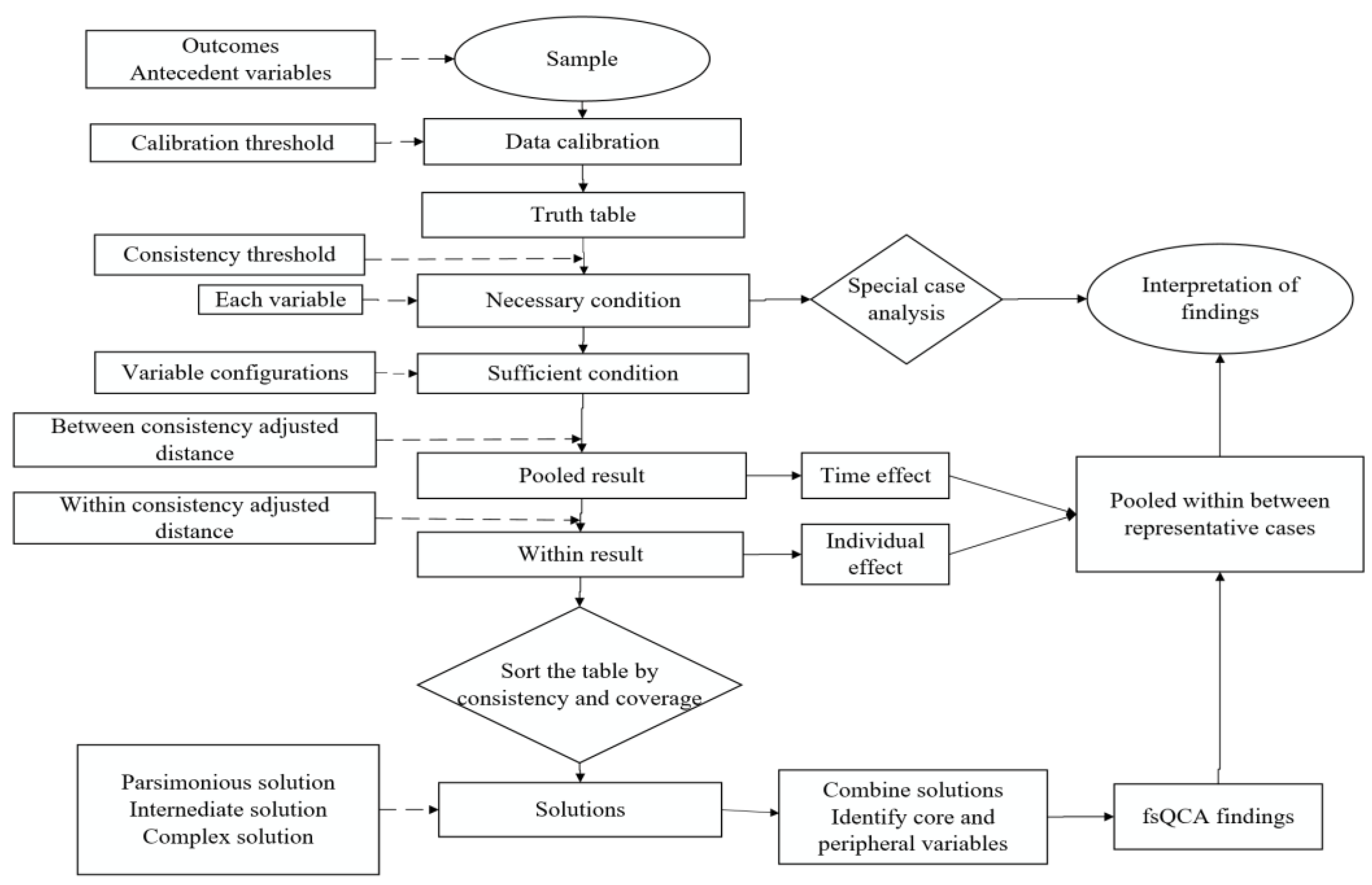
Figure 1. Steps in the dynamic fsQCA method.
Sustainability 17 05931 g001
Figure 2. Research framework.
Sustainability 17 05931 g002
Figure 3. Efficiency of forest carbon sink in China from 2008 to 2022.
Sustainability 17 05931 g003
Figure 4. Temporal trends in forest carbon sink efficiency across Chinese provinces.
Sustainability 17 05931 g004
Figure 5. Spatial distribution of forest carbon sink efficiency in China.
Sustainability 17 05931 g005
Figure 6. Three-dimensional kernel density map of forest carbon sink efficiency in China.
Sustainability 17 05931 g006
Figure 7. Index change of forest carbon sink efficiency in China.
Sustainability 17 05931 g007
Figure 8. Decomposition of forest carbon sink efficiency index change in China.
Sustainability 17 05931 g008
Figure 9. Scatter plot group diagram of necessity condition test.
Sustainability 17 05931 g009
Figure 10. Trends in “between consistency”.
Sustainability 17 05931 g010
Table 1. Forest carbon sink efficiency.
VariableIndexIndicator Interpretation (Units)Unit
Input LaborYear-end employment in the forestry sectorPeople
LandForest area103 hm2
CapitalTotal amount of investment in fixed assets103 CNY
Desirable
output
EconomyTotal value of the primary forestry industry103 CNY
Carbon sinkForest carbon sinkTon
Undesirable outputCarbon source Carbon dioxide emissionsTon
Table 2. Descriptive statistics of indicators.
VariableMeanS.DMinMax
Input Year-end employment in the forestry sector 39,273.3555,711.91496234,181
Forest area706.89615.111.892614.85
Total amount of investment in fixed assets600,253.981,196,293.7451810,861,358
Desirable output Total value of the primary forestry industry19,313,982.5327,734,177.8223,999374,085,252
Forest carbon sink49,11259,618.3438.51228,537.41
Undesirable outputCarbon dioxide emissions153.24110.365.33777.16
Table 3. Indicators of influencing factors of forest carbon sink.
CategoryIndex
(Abbreviation)
Indicator Description (Units)Indicator
Direction
Natural
endowment
Forest coverage (FC)
Precipitation (PRE)
Ratio of forest area to total land area (%)+
+
Total annual precipitation (mm)
Social
development
Total value of the primary forestry industry (TPFI)Total forestry primary industry
(104 CNY)
+
Gross regional domestic product (GDP)108 CNY+
Year of education (YOE)Years of education for forestry practitioners (years)+
Forest
management
Forestry pest control rate (FPCR)%+
Fire-damaged area (FDA)Area of forest destroyed by fire (ha)-
Table 4. Descriptive statistics of influencing factors.
VariableDescriptive Statistics
MeanS.DMinMax
Result variableFCSE1.101.780.0215.12
Condition variableFC32.7117.892.9766.84
PRE916.76514.6455.902432.6
TPFI6,233,096.325,369,863.452328424,215,489
GDP24,171.5121,873.23 896.9129,118.6
YOE14.210.7110.5615.67
FPCR76.66 21.878.45100
FDA695.961799.630.1517780.99
Table 5. Calibration results of variables.
Variable CategoryVariableFull MemberCrossover PointFull Non-Member
Outcome variableFCSE1.2020.6530.339
Antecedent variableFC46.06835.15516.723
PRE1279.1822.625491.725
TPFI9,061,2034,771,5432,018,558
GDP31,460.7517,569.29937.6
YOE14.7614.32813.729
FPCR93.84882.89566.67
FDA578.708133.9729.222
Table 6. Index and its decomposition.
RegionFCSE Change Index
MLECTC
Beijing0.820.711.15
Tianjin0.540.371.45
Hebei1.151.011.14
Shanxi0.940.591.59
Inner Mongolia1.040.651.6
Liaoning0.810.761.07
Jilin1.461.121.3
Heilongjiang1.270.991.28
Shanghai1.291.11.17
Jiangsu1.531.560.98
Chekiang0.380.40.94
Anhui1.080.791.37
Fujian1.080.971.12
Jiangxi1.31.690.77
Shandong0.90.81.12
Henan0.820.661.24
Hubei1.441.161.24
Hunan1.111.051.06
Guangdong1.201.001.20
Guangxi1.181.001.18
Hainan0.740.760.98
Chongqing1.041.011.03
Sichuan1.070.961.11
Guizhou1.341.261.06
Yunnan1.010.931.09
Shanxi1.141.011.13
Gansu0.810.312.60
Qinghai1.030.971.06
Ningxia0.350.750.46
Xinjiang0.520.451.16
Western remote region1.000.831.21
Central inland region1.230.971.27
Eastern coastal region0.990.881.12
Mean value1.090.901.21
Table 7. Moran’s I of China’s forest carbon sink efficiency.
YearMoran’s IpZ
2008−0.070.27−0.61
2009−0.070.21−0.8
2010−0.080.15−1.06
2011−0.080.2−0.85
2012−0.070.17−0.95
2013−0.070.15−1.05
2014−0.070.12−1.16
2015−0.050.45−0.13
2016−0.090.25−0.68
20170.030.230.75
20180.040.170.96
2019−0.040.49−0.03
20200.050.250.68
2021−0.010.410.23
20220.130.051.61
Table 8. Necessity of each variable.
VariableHigh FCSE
Pooled ConPooled CovBetween Con Adjusted DistanceWithin Con Adjusted Distance
FC0.560.5840.0850.679
~FC0.5160.5250.1060.69
PRE0.5750.6010.0890.644
~PRE0.4930.5010.1150.69
TPFI0.5470.5660.3360.529
~TPFI0.5310.5450.3660.61
GDP0.5570.5880.2260.633
~GDP0.5140.5170.2470.621
YOE0.5660.5890.5240.5
~YOE0.5080.5180.5580.575
FPCR0.6160.6210.1190.529
~FPCR0.4680.4930.1870.569
PDA0.5070.5410.230.575
~PDA0.5720.5690.1920.581
Note: Con stands for consistency, Cov stands for coverage.
Table 9. Configuration analysis results.
VariableConfiguration Analysis—High
Configuration 1Configuration 2Configuration 3
Forest coverage
Precipitation
Total value of the primary forestry industry
Gross regional domestic product
Year of education
Forestry pest control rate
Fire-damaged area
Consistency0.8240.8280.753
PRI0.7550.7680.534
Coverage0.1750.1790.091
Unique coverage0.0780.1020.000
Between consistency adjusted distance0.1230.1620.115
Within consistency adjusted distance0.3740.3280.311
Overall consistency0.822
Overall PRI0.771
Overall coverage0.318
Note: ● and ⮾ represent the core condition, and the space indicates that this condition does not affect this configuration.
Table 10. Average regional coverage.
RegionConfiguration 1Configuration 2Configuration 3
Eastern coastal region0.310.2720.164
Central inland region0.3270.2030.363
Western remote region0.1170.2490.198
Table 11. Comparison of original consistency results before and after adjustment.
VariableThe Frequency Is 4The Frequency Is 5
Configuration 1Configuration 2Configuration 3Configuration 1Configuration 2
FC
PRE
TPFI
GDP
YOE
FPCR
FDA
Consistency0.8240.8280.7530.8240.828
PRI0.7550.7680.5340.7550.768
Coverage0.1750.1790.0910.1750.179
Unique coverage0.0780.10200.0380.126
Between consistency adjusted distance0.8220.827
Within consistency adjusted distance0.7710.776
Overall consistency0.3180.3
Note: ● and ⮾ represent the core condition, and the space indicates that this condition does not affect this configuration.
Disclaimer/Publisher’s Note: The statements, opinions and data contained in all publications are solely those of the individual author(s) and contributor(s) and not of MDPI and/or the editor(s). MDPI and/or the editor(s) disclaim responsibility for any injury to people or property resulting from any ideas, methods, instructions or products referred to in the content.