Nomogram-Based Rainwater Harvesting Design for a Sustainable Residential Water Supply

Abstract

Water scarcity is a critical issue exacerbated by climate change, urbanization, and population growth, particularly in regions with insufficient water infrastructure. Rainwater harvesting (RWH) systems offer a sustainable solution to mitigate water shortages by collecting and storing rainwater for non-potable uses. This study focuses on the design, efficiency, and reliability of RWH systems in residential environments, with an emphasis on optimizing the sizing of storage volumes and collection areas. Using a behavioural simulation model, we generate nomograms that facilitate the design of RWH systems by analyzing the interactions among storage capacity, collection area, rainfall patterns, and water demand. Specifically, this paper evaluates the effectiveness of RWH systems through efficiency and reliability metrics such as water savings, mains reliance, overflow discharge, and system reliability. The proposed procedure integrates stochastic rainfall and water demand data, including a detailed analysis of toilet usage, in order to simulate the performance of RWH systems across different time scales. Case studies in Italy and Denmark are used to assess the influence of climatic differences on system performance. The findings provide a comprehensive methodology for RWH system design, and offer valuable insights into improving a sustainable water management strategy.

1. Introduction

As indicated in a report by the United Nations’ WWAP [1], global water demand is increasing by about 1% per year due to various factors such as population growth, economic development, and changing consumption patterns. This trend is expected to continue over the next two decades. According to the same document, although agricultural use remains the largest, industrial and domestic water demand is increasing more rapidly, particularly in developing and emerging economies. At the same time, climate change is affecting the hydrological cycle on a global scale, enlarging disparities between wet and dry regions.

This pressing issue has spurred interest in sustainable water management practices, including rainwater harvesting (RWH) systems, which provide a practical alternative to traditional potable water supplies. RWH systems capture and store rainwater for non-potable uses such as irrigation, toilet flushing, and laundry.

The performance of these systems depends on several key factors, including reservoir capacity, collection area, local rainfall patterns, and user demand. Data from the Statistical Office of the European Commission (EUROSTAT) [2] indicate that an increasing number of countries experience water scarcity during the spring, with even more pronounced shortages in the summer.

The Italian National Institute of Statistics (ISTAT) report [3,4], released annually on World Water Day, carries out water statistics from various surveys to present a detailed overview of the country’s water dynamics. The goal is to provide users with an integrated view of water-related statistics, with a particular focus on territory, population, and economic activities. Latest reports based on data up to 2024 show some fragilities. Drinking water supply in Italy comes mainly from withdrawals from aquifers through springs and wells. Over 50% of drinking water sources come from springs, contributing to 36.2% of total water withdrawal, with a volume of 3.3 billion cubic metres [4]. Italy is one of the European countries with the highest withdrawal of fresh water for drinking use [3]. In recent years, drinking water restrictions have impacted parts of southern Italy, occasionally leading to daily supply suspensions or reductions. Water distribution followed a weekly rotation based on the area. Substitute water truck services were frequently employed to mitigate these shortages. The crisis worsened in 2024, affecting more towns and extending the duration and severity of emergency measures. Consequently, restrictions became even stricter and more frequent. The main factors contributing to the low or insufficient availability of water resources in these regions include the severe obsolescence of the water infrastructure networks, significant deficits in precipitation compared to the past climatological average, higher-than-average temperatures, and reduced reservoir inflows [4]. Additionally, climate change is also negatively impacting other parts of Italy, leading to the depletion of aquifers and a reduction in available water flows [5,6].

This highlights the potential of effective water management and conservation strategies in addressing these challenges. By utilizing rainwater, an often-underappreciated resource in modern buildings, RWH systems can reduce reliance on potable water and create reserves for drought periods. In many water-stressed regions, the issue is not necessarily insufficient rainfall but rather the lack of adequate systems and technologies for its capture and storage [7].

Rainwater collection tanks can be easily sized by using specific technical standards. In Italy, the UNI/TS 11445:2012 standards [8] are available, while the German E DIN 1989-1:2000-12 standards [9] are also commonly applied. Both rely on rainfall data and average annual water requirements but do not account for the temporal distribution of rainfall and water consumption. These standards are mainly used for the preliminary sizing of tanks, whose efficiency and reliability can be validated by subsequent simulation models, among which behavioural models are the most commonly used [10].

Behavioural models simulate the performance of a water collection tank over time by routing inflows and outflows through algorithms that represent the tank’s operational behaviour. The RHW’s operation can be simulated over several years, using the input data of rain and consumption in time series form. These data are based on time intervals such as hours, days, or months to model the mass flow through the system.

Jenkins et al. [11] introduced the Yield After Spillage (YAS) model, which is a simple behavioural approach that accounts for rainfall inputs and water withdrawals based on demand at each time step. In the same study, Jenkins et al. [11] also introduced the Yield Before Spillage (YBS) model as a modification of the YAS model.

Fewkes [10] also evaluated the efficiency of rainwater harvesting (RWH) systems at five UK sites using the YAS and YBS behavioural models. The study examined how model performance varies considering the monthly or daily time scales for rain and demand series.

A behavioural model was also implemented by Campisano et al. [12,13] to assess the inflow, outflow, and change in storage volume of a rainwater harvesting system using daily mass balance simulations based on historical rainfall observations. The performance of the RWH system under various climate and operational conditions was examined as a function of non-dimensional parameters, one of which was introduced by these authors to allow an improved description of the rainfall patterns.

Liuzzo et al. [14] evaluated the performance of a proposed RWH tank for a single household in a residential area using rain data from over 100 sites in Sicily. Annual reliability curves for the system as a function of Mean Annual Precipitation were derived using the YAS behavioural model. With a resampling method, model uncertainty was assessed, and a cost–benefit analysis estimated the payback time.

Overall, many studies on RWH focus on developing design criteria that optimize system performance. These results are heavily influenced by the geographic and climatic conditions of each site, and many authors also address the economic aspect by aiming to minimize the overall cost of the water supply [15]. The economic benefits of these systems have been evaluated more comprehensively by also incorporating environmental impact assessments through life cycle analysis (LCA). Through this approach, the environmental effects of producing drinking water via conventional urban supply systems have been compared with those of centralized systems that integrate rainwater harvesting [16].

More recently, Piazza et al. [17] present an updated analytical–probabilistic approach to predict the probability of rainwater reuse for toilet flushing. The method incorporates water demand as a random variable, simplifies the representation of antecedent rainfall contributions, and exploits a cloud streaming platform for the statistical analysis and forecasting of users’ consumption. The proposed equations have been applied to a case study in a residential neighbourhood of Palermo (Sicily) and have been supported by a field campaign.

This study focuses on the design, efficiency, and reliability of rainwater tanks in residential environments. It aims to propose a user-friendly methodology for the sizing of the storage volume and the collection area, ensuring pre-established efficiency and reliability values. Specifically, the application of a ‘hybrid stochastic–deterministic simulation model’ allows nomograms to be obtained, through which it is possible to simultaneously determine storage volumes and collection areas. Moreover, our proposed approach represents a descriptive model, i.e., we model and interpret observed data and data from the literature in order to support RWHS design. Three different time scales, monthly, daily, and hourly, are used for the rainfall and water demand time series. The water demand series is related to toilet use only and is generated with a stochastic model. The rainfall series derives from both rainfall measurements and data generated through a properly calibrated model. The effects of rainfall patterns are examined considering rainfall data from two areas with very different climatic characteristics.

The following is a summary of the structure of this work: Section 2 describes the behavioural model, stochastic input models for water demand and rainfall depth, and the dimensionless parameters through which the input and output data are generalized. In Section 3, the selected case studies in Italy and Denmark are shown, while the obtained results are discussed in Section 4. Finally, Section 5 provides concluding remarks.

2. Methods

2.1. Simulation Model for Rainwater Harvesting (RWH) Systems

Numerous models have been developed to analyze the performance of rainwater harvesting (RWH) systems [10]. An important contribution to this topic was made by Jenkins et al. (1978) [11], who introduced a behavioural modelling approach along with two key algorithms for characterizing the performance of rainwater storage tanks: Yield After Spillage (YAS) and Yield Before Spillage (YBS). The following outlines the equations that govern these algorithms, based on discrete time intervals Δt (e.g., hourly, daily, or monthly):

$$\begin{gathered} Y\left({∆t}_i\right)=\mathit{min}\left\{\begin{array}{c}D\left({∆t}_i\right)∆t\\ V\left({∆t}_{i-1}\right)\end{array}\right. \\ V\left({∆t}_i\right)=\mathit{min}\left\{\begin{array}{c}V\left({∆t}_{i-1}\right)+A\ast I\left({∆t}_i\right)∆t-Y\left({∆t}_i\right)\\ S-Y\left({∆t}_i\right)\end{array}\right. \end{gathered}$$

(1a)

$$\begin{gathered} Y\left({∆t}_i\right)=\mathit{min}\left\{\begin{array}{c}D\left({∆t}_i\right)∆t\\ V\left({∆t}_{i-1}\right)+A\ast I\left({∆t}_i\right)∆t\end{array}\right. \\ V\left({∆t}_i\right)=\mathit{min}\left\{\begin{array}{c}V\left({∆t}_{i-1}\right)+A\ast I\left({∆t}_i\right)∆t-Y\left(t\right)\\ S\end{array}\right. \end{gathered}$$

(1b)

where

$Y(∆t)$: Yield from store ([L³]) during time interval $∆t$;

$D(∆t)$: Water demand ([L³/T]) during time interval $∆t$;

$V\left(∆t\right)$: Volume in store ([L³]) during time interval $∆t$;

$I\left(∆t\right)$: Rainfall intensity ([L/T]) during time interval $∆t$;

A: Catchment area ([L²]);

S: Storage capacity ([L³]).

The main distinction between these models lies in the different initial conditions they consider. The following can be determined, as already mentioned into the introduction:

• In the YAS model, the water yield at the i-th time step is derived only from the stored volume from the preceding time step.
• In the YBS model, the water yield at the i-th time step depends on the residual storage from the previous step integrated with the rainfall input at the current time.

Therefore, under dry or low-rainfall conditions, the maximum volume that can be retained in the reservoir using the YAS algorithm does not reach the full storage capacity S, unlike the YBS approach. The YAS algorithm is intentionally designed to yield conservative performance estimates that are independent of the model’s temporal resolution, making it more appropriate for design applications compared to the YBS algorithm [18].

The YAS system, defined by Equation (1a), involves four unknowns in the design phase: S, A, V($∆t$), and Y($∆t$). The demand $D\left(∆t\right)$ and rainfall intensity $I\left(∆t\right)$ values are either obtained from field measurements or calculated through suitable simulation models.

Behavioural simulations are carried out by investigating different combinations of catchment area A and storage capacity S, which are synthetized with two key ratios frequently cited in the literature: the storage fraction $sf={\displaystyle \frac{S}{\left(A\ast \tilde{I}\right)}}$ and the demand fraction $df={\displaystyle \frac{(\tilde{D}\ast t_{sim})}{\left(A\ast \tilde{I}\ast t_{sim}\right)}}$, with $\tilde{D}$ and $\tilde{I}$, respectively, representing mean water demand and mean rain intensity over the simulation period $t_{sim}$. The storage period $sp={\displaystyle \frac{S}{\tilde{D}=sf/df}}$ is also considered.

The storage fraction $sf$, expressed as a time measure, represents the duration required to fill the volume S, based on the catchment area A and the average rainfall intensity $\tilde{I}$. The storage period $sp$, also expressed as a time measure, represents the duration required to deplete the volume S under average water demand conditions $\tilde{D}.$ The demand fraction $df$, a dimensionless parameter, represents the ratio of the volume of water required by the user to the total volume of rainfall over the simulation period $t_{sim}$.

To constrain the behavioural simulation within specific design conditions, the order of magnitude for the storage volume (S) and collection area (A) is estimated based on relevant technical standards, such as UNI/TS 11445:2012, and the spatial constraints of the project site. Subsequently, using user demand and rainfall data, the simulation model is employed to calculate the two remaining unknowns, V(Δt) and Y(Δt), across different combinations of S and A, which vary around their initially estimated values.

A further review of the results identifies four critical parameters essential for evaluating the system’s performance. Three of these parameters pertain to the system’s efficiency, while the fourth one relates to its reliability. These parameters are as follows: water saving ($W_S$), mains ($M$), overflowing discharge ($O_D$), and reliability ($Re$).

Water saving efficiency serves as a metric for quantifying the extent of mains water conserved relative to the overall demand, as articulated in Equation (2).

$$W_S(\%)={\displaystyle \frac{{\sum }_{t=1}^{t_{sim}}Y(∆t)}{{\sum }_{t=1}^{t_{sim}}\left(D\right(∆t)\ast ∆t)}}\ast 100$$

(2)

Mains is a measure of the volume supplied by the mains and is given by Equation (3):

$$M(\%)={\displaystyle \frac{{\sum }_{t=1}^{t_{sim}}\left(D\right(∆t)\ast ∆t)-Y\left(t\right)}{{\sum }_{t=1}^{t_{sim}}\left(D\right(∆t)\ast ∆t)}}\ast 100$$

(3)

Overflow discharge represents a quantifiable assessment of the volume of surplus rainwater that can be redirected for alternative applications, as delineated by Equation (4):

$$O_D(\%)={\displaystyle \frac{{\sum }_{t=1}^{t_{sim}}{Q}_D}{{\sum }_{t=1}^{t_{sim}}(A\ast I\left({∆t}_i\right)∆t)}}\ast 100$$

(4)

where $Q_D$ is the volume discharged as overflow from the storage tank [11].

Reliability is estimated by using Equation (5):

$$\mathit{Re}(\%)={\displaystyle \frac{n}{N}}\ast 100$$

(5)

where $n$ is the number of days when demand is fully met while $N$ is the total number of days in the simulation [7].

Demand and rainfall data can originate from field measurements or be generated using appropriate simulation models. In the latter case, this study employs two distinct stochastic models based on rectangular pulses: the Poisson Rectangular Pulse (PRP) model for simulating water demand (Section 2.2), and the Neyman–Scott Rectangular Pulse (NSRP) model for simulating precipitation (Section 2.3).

2.2. Water Demand Model

Over the last few decades, instantaneous water demand models have become increasingly widespread: they represent consumption as a stochastic process defined by the parameters that physically characterize individual usage events. In particular, the stochastic Poisson with Rectangular Pulses (PRP) model [19,20] introduces three key parameters, intensity, duration, and frequency, for each elementary consumption pulse. Furthermore, PRP must preserve the distinctive features of the phenomenon across different spatial and temporal aggregation scales, with particular attention given to total delivered volumes and peak consumption factors.

As described by Buchberger et al. [21], home occupants in each residence can be modelled as customers, while water fixtures and appliances are represented as servers. Customer arrivals are modelled as a Poisson process with a rate parameter λ. Each instance of server usage is represented by a rectangular pulse characterized by a specific duration and intensity. Since these pulses have finite durations, events that begin at different times may briefly overlap. During these overlapping intervals, the total water demand intensity is the sum of the individual pulse intensities. Generally, durations and intensities are mutually independent and drawn from predefined probability distributions.

However, in this context, we focus solely on toilet usage, which is assumed to have a constant duration and intensity whose values were selected to reflect an average among contemporary flushing systems, including those with flush cut-off mechanisms or dual-flush buttons. These systems typically offer two modes: a short flush (4–6 L) and a full flush (9–12 L). For simplicity and conservatism, a constant flush volume of 9 L was adopted, disregarding mode variability. This assumption errs on the side of safety by overestimating water usage. Additionally, a fixed flush duration of 3 min was assumed. The frequency of toilet flushing was modelled by segmenting the day into four discrete time intervals, each corresponding to a distinct flushing frequency, as reported in

Table 1. Per capita toilet flush number and corresponding PRP frequency.

Time Interval	Number of Hours	Number of Flushes per Day	Mean Frequency λ (1/s)
00:00–06:00	6	4	4.63 × 10−5
06:00–10:00	4	12	1.39 × 10−4
10:00–18:00	8	6	6.94 × 10−5
18:00–24:00	6	9	1.04 × 10−4
00:00–24:00	24	7.25	8.39 × 10−5

. The delineation of these intervals was derived from the daily domestic water demand distribution curve presented by Alam Imteaz and Boulomytis [18]. Then, based on the weighted average, each person flushed the toilet approximately 7.25 times per day.

Liuzzo et al. [14], based on a statistical analysis of water consumption data collected from seven families in Palermo (Sicily) over a three-year monitoring period, reported an average number of toilet flushes of 5.32, with a root mean square error (RMSE) of 2.927. The value used in this study, therefore, falls within the upper range of the variability interval identified by those authors.

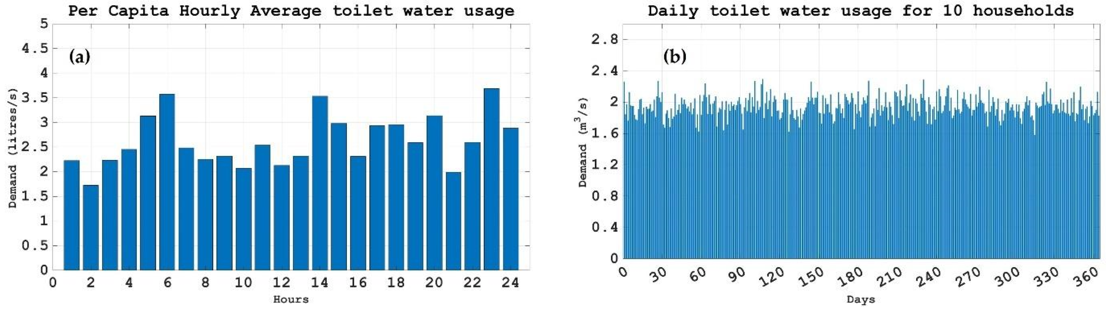
In the case studies analyzed in this research, which are distinguished by varying geographical locations and climatic conditions, the water demand associated with toilet (WC) usage was consistently evaluated based on a scenario involving 10 residential units, each comprising three inhabitants.

The demand simulation was implemented in MATLAB, (version R2024a Update4) yielding the total hourly water consumption over the whole simulation period (Section 4.3). In Figure 1 we represent a generic day and a generic year. The model estimates an average daily water demand of 1.9 m³ for the ten users, equivalent to approximately 65 L per capita per day. According to published data, the flushing of toilets accounts for more than 30% of domestic water use [22]. Assuming this proportion holds, the implied total domestic water use in this case would be approximately 217 L per capita per day.

2.3. Rainfall Model

The availability of long high-resolution rainfall depth series is crucial for accurately estimating rainfall features, which are essential for designing urban infrastructures. However, in many regions worldwide, observed hourly or sub-hourly rainfall data from rain gauges often lack long sample sizes (see, for instance, Figure 1 in [23]). Recent studies highlight the effectiveness of Stochastic Rainfall Generators (SRGs) in accurately simulating long rainfall series that are suitable for hydrological spatial and temporal scales [24]. Many SRGs model the clustering structure of rainfall fields [25,26,27] and can generate storm events that are randomly distributed in both space and time. Classical SRGs include models such as Poisson White Noise (PWN), Poisson Rectangular Pulse (PRP), Neyman–Scott White Noise (NSWN), Neyman–Scott Rectangular Pulse (NSRP), Bartlett–Lewis Rectangular Pulses (BLRP), and Bartlett–Lewis Instantaneous Pulse (BLIP) [28,29,30,31,32,33,34,35,36]. In particular, De Luca and Petroselli [34] emphasized the possibility of calibrating SRGs using summary statistics derived from annual maxima series (i.e., parameters of Intensity–Duration–Frequency (IDF) curves), annual and seasonal cumulative rainfall totals, and the annual number of wet days (i.e., days with at least 1 mm of cumulative depth), which are generally more accessible than high-resolution rainfall data typically used for calibrating SRG models.

Then, in the master’s thesis of the second author in this work, a classical NSRP model [37] was implemented in MATLAB (version R2024a Update4 similarly to the other modules briefly described in the previous Section 2.1 and Section 2.2), in which the following occurred:

• All the NSRP parameters [31,32] presented a seasonal variability which was modelled by using goniometric series.
• For the selected case studies (see Section 3), the calibration was carried out by minimizing the differences among the observed and simulated (from a 500-year generated stationary series) summary statistics (Mean Annual and Seasonal Precipitation, Mean Annual Number of Wet Days, parameters of IDF curves).

Moreover, an important key aspect must be highlighted before the results discussion in Section 4. As reported in the following Section 3 (Materials), sample sizes of less than 15 years characterize the observed rainfall data for the investigated areas, but this length is not sufficient to assess possible effects due to climate changes [38], and so a cyclo-stationary version of the NSRP model (i.e., with parameters having only a seasonal variability) is adopted.

Clearly, a transient version of the NSRP model can be taken into account for the further development of the proposed methodology, as also mentioned in Section 5 (Conclusions).

3. Materials

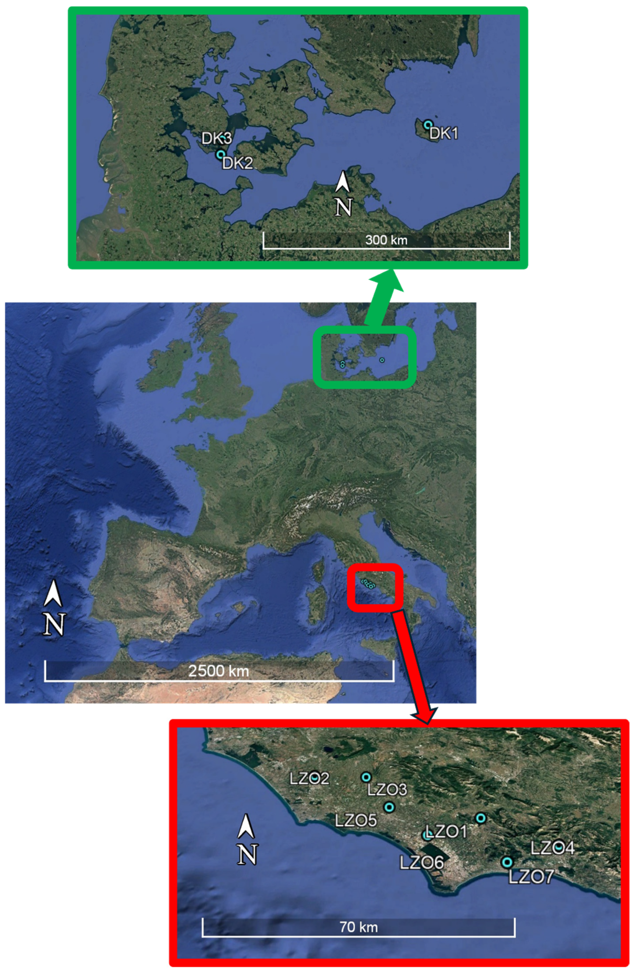
Two distinct areas were analyzed in this study (Figure 2):

• Pontino zone, located in the Lazio region (Central Italy);
• Two islands in Denmark, namely Langeland and Bornholm.

The Pontino zone is characterized by altitudes slightly above sea level, ranging from a few metres to about 70 m. Rainfall daily data were provided upon request by the Civil Protection Agency of the Lazio Region . They cover the 13-year period from 1 January 2011 to 31 December 2023.

Table 2. Geographical features of the investigated rain gauges in the Lazio region (central Italy).

ID	Rain Gauge Name	Municipality	Longitude (°)	Latitude (°)	Elevation (m a.s.l.)
LZO1	Amaseno a Fossanova	Sonnino	13.1944	41.4333	16
LZO2	Aprilia	Aprilia	12.6483	41.5939	75
LZO3	Cisterna di Latina	Cisterna di Latina	12.8233	41.5894	69
LZO4	Fondi	Fondi	13.4189	41.3422	1
LZO5	Latina	Latina	12.9058	41.4714	17
LZO6	Rio Cassano	Sabaudia	13.0264	41.3728	20
LZO7	Terracina	Terracina	13.2558	41.2867	18

and

Table 3. Pluviometric features of the investigated rain gauges in the Lazio region (central Italy).

ID	MAP (mm)	MANWD (Days)	DJF (mm)	MAM (mm)	JJA (mm)	SON (mm)
LZO1	957	84	277	158	148	374
LZO2	855	81	254	138	111	351
LZO3	931	77	272	164	128	367
LZO4	936	76	272	158	131	375
LZO5	844	76	259	124	107	355
LZO6	920	81	264	133	132	391
LZO7	844	80	245	122	115	360
Mean Values	898.1	79.3	263.3	142.4	124.6	367.6

summarize, respectively, the geographical and pluviometric features of the seven investigated rain gauges, in terms of latitude, longitude, and elevation, and of the Mean Annual Precipitation (MAP); Mean Annual Number of Wet Days (MANWD); and mean seasonal precipitation for December–January–February (DJF), March–April–May (MAM), June–July–August (JJA), and September–October–November (SON). Concerning the parameters of the Intensity–Duration–Frequency (IDF) curves for sub-daily scales, authors considered the values derived from the methodology of the Flood Evaluation project [39].

Similarly, Danish rainfall series were extracted by using a QGIS plugin created by the Danish Meteorological Institute (DMI). The data cover a 14-year period, i.e., from 1 January 2011 to 31 December 2024, for three rain gauges indicated in

Table 4. Geographical features of the investigated rain gauges in Denmark.

ID	Rain Gauge Name	Municipality	Longitude (°)	Latitude (°)	Elevation (m a.s.l.)
DK1	Østerlars	Bornholm	14.9683	55.1630	94
DK2	Søndenbro	Langeland	10.7094	54.7567	7
DK3	Rudkøbing	Langeland	10.7234	54.9463	8

and

Table 5. Pluviometric features of the investigated rain gauges in Denmark.

ID	MAP (mm)	MANWD (Days)	DJF (mm)	MAM (mm)	JJA (mm)	SON (mm)
DK1	679	110	225	189	92	171
DK2	604	103	148	162	154	139
DK3	561	99	157	157	112	126
Mean Values	614.7	104.0	176.7	169.3	119.3	145.3

. With regards to the parameters of the IDF curves for sub-daily scales, the authors adopted the regional curves proposed in Madsen et al. [40,41]. The Danish islands of Langeland and Bornholm, located in the Baltic Sea, present a gently undulating terrain (with elevations generally below 200 m a.s.l.) and a temperate maritime climate, characterized by mild winters and cool summers.

From the analysis of Table 3 and Table 5, it is clear that (for the investigated periods), the Pontino zone in the Lazio region presents larger values of MAP (898.1 mm as mean areal value) with respect to the Danish area (614.7 mm as mean areal value).

On the contrary, greater MANWD and a more uniform seasonal distribution of rainfall depths are associated with Denmark. The seasonal rainfall distribution in Pontino shows peaks during the autumn and winter months, with average areal accumulated values which are more than double with respect to the summer months; this disparity is not observed in the Danish climate, where there is an average areal difference of less than 60 mm (i.e., 10% of the correspondent MAP areal value) between the wettest and dryest seasons (winter and summer, respectively).

The mean areal summary statistics from each of the two station groups (see the last row of Table 3 and Table 5 for annual and seasonal indicators) were used for the calibration of the adopted NSRP model; two synthetic rain datasets, representative of the corresponding climatically homogeneous regions, were generated and used as climatic input for the YAS model (Section 4).

4. Results and Discussion

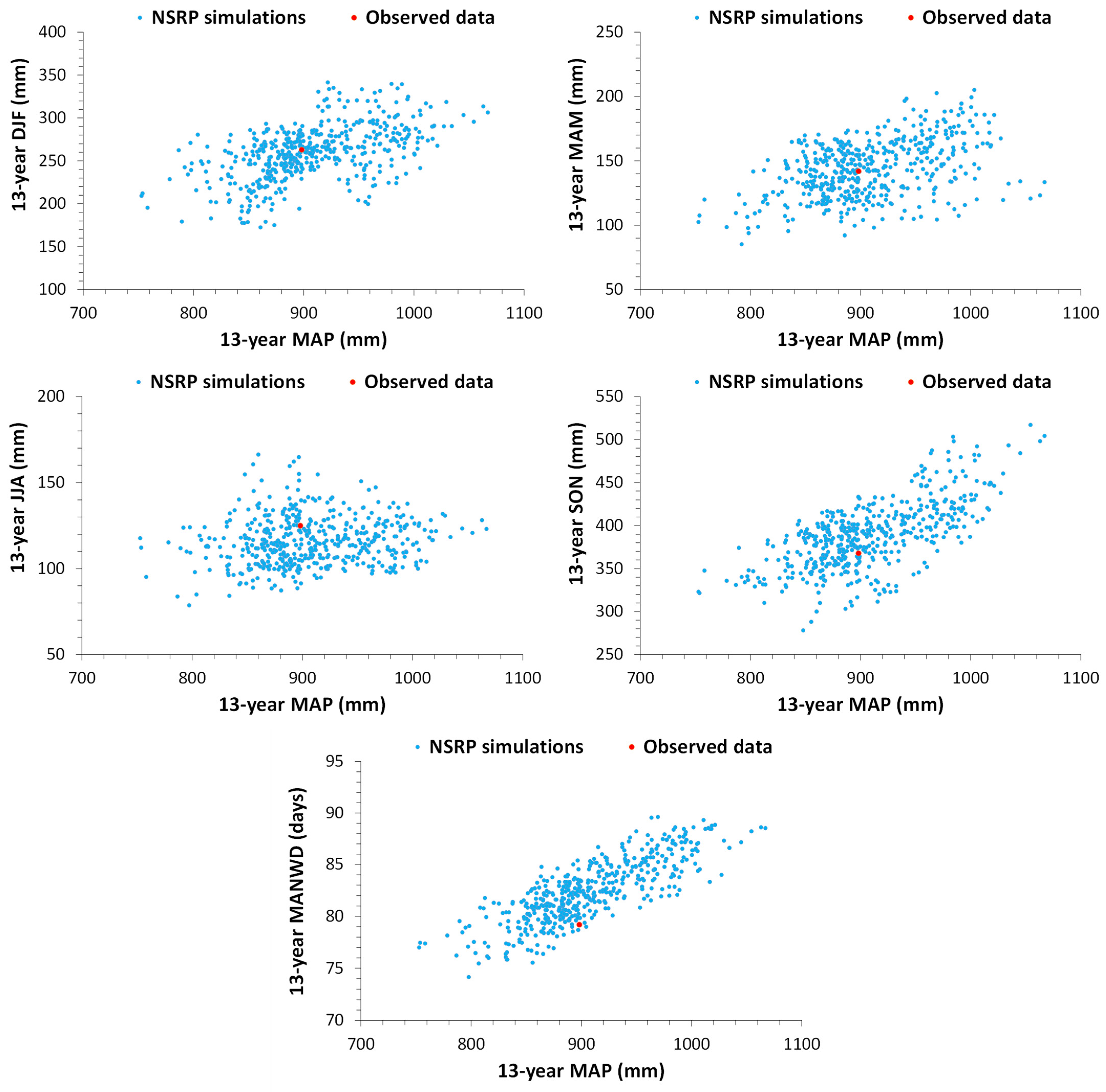
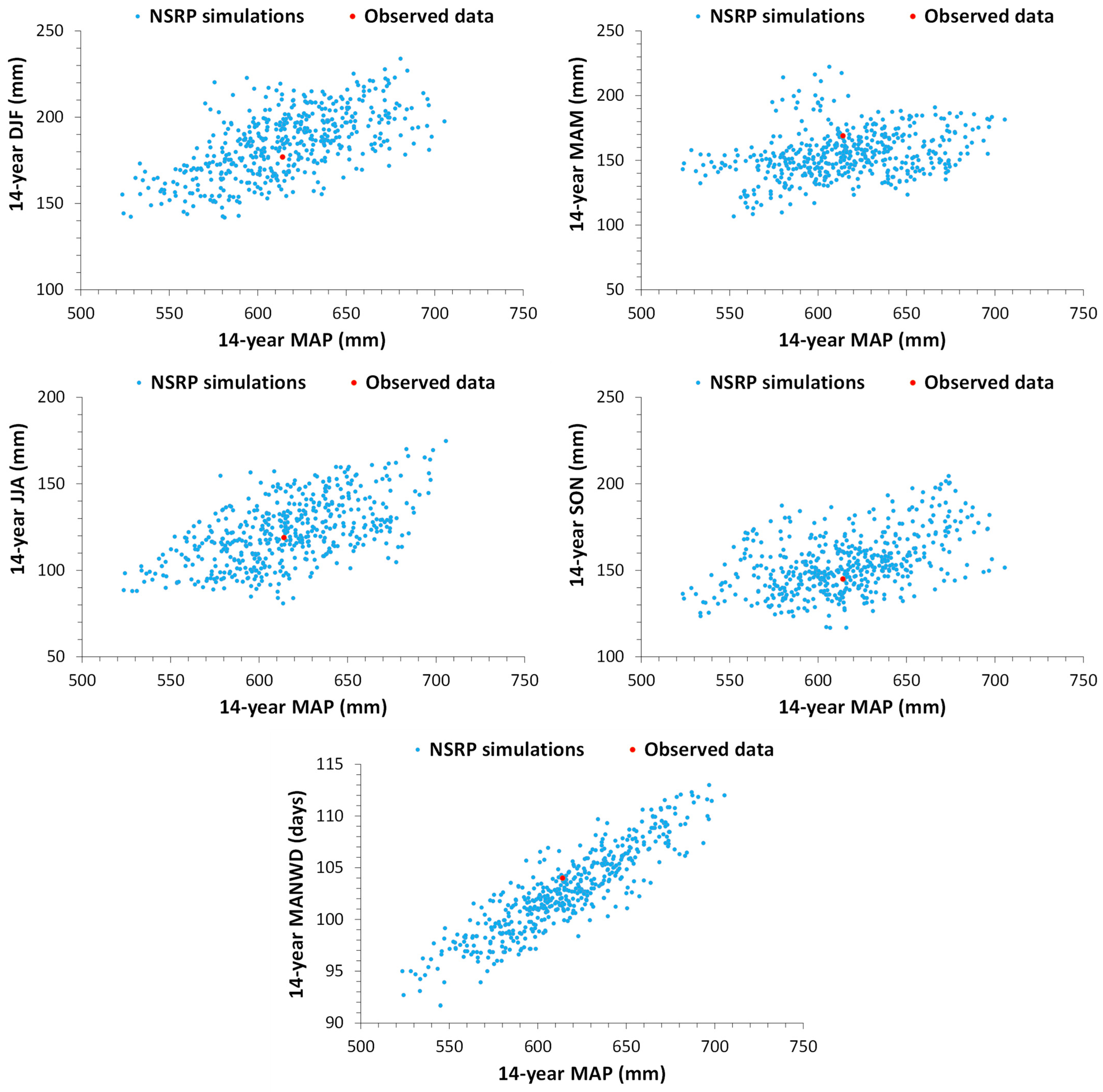
4.1. Performances of NSRP Model

For the investigated areas (Section 3), the performances of the calibrated NSRP model were analyzed by considering 500 simulations of hourly time series, each one with a length of 13 years (for Lazio area) and 14 years (for Danish area), respectively.

In detail, we compared 13 (14)-year summary statistics from the whole set of simulations with the observed ones, in terms of MAP, MANWD, and mean seasonal precipitation for DJF, MAM, JJA, and SON.

Figure 3 and Figure 4 highlight that the “clouds” of the NSRP summary statistics undoubtedly comprise the observed rainfall features for both study cases, and then the adopted SRG model can clearly be used for the successive analyses, in which a 500-year synthetic rainfall hourly series for each investigated zone is generated and adopted as climatic input for the YAS model (Section 4.2 and Section 4.3).

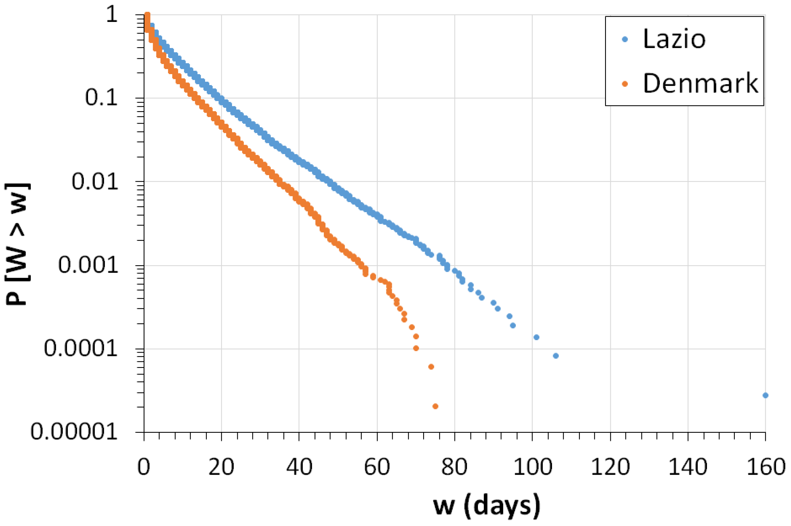
Moreover, from both the 500-year synthetic series for Lazio and Denmark it is possible to derive the probability distribution of the waiting time $W$ (expressed in days) between two consecutive rainy events, where a rainy event is defined as a set of consecutive wet days. Figure 5 represents the exceedance probability $P[W>w]$ on the vertical axis; for any w value of the random variable W, $P[W>w]$ is always greater for the investigated Lazio area. In details,

Table 6. Percentiles of waiting time W between two consecutive rainy periods, derived from NSRP simulations.

$\mathit{P}\left[\mathit{W}>\mathit{w}\right]$	$\mathit{w}$ (Days)
	Lazio	Denmark
0.01	48	35
0.05	27	20
0.10	19	14

reports the percentiles for $P\left[W>w\right]=0.01, 0.05, 0.10$.

For the successive analyses with the nomograms (Section 4.3), the authors will consider the percentiles associated with $P\left[W>w\right]=0.05$.

4.2. Simulation Time Resolution

To evaluate the impact of temporal resolution on model behaviour, 500-year simulations were conducted using synthetic inputs of rain and water demand aggregated at hourly, daily, and monthly intervals.

The use of the highest resolution, e.g., hourly scale, allows for a more accurate representation of storage tank efficiency and offers a more realistic depiction of system dynamics. However, it is essential to evaluate whether this increased temporal detail significantly influences the simulation outcomes. High-resolution data typically come with increased resource demands—not only due to limited data availability but also because of the larger file sizes and higher computational requirements.

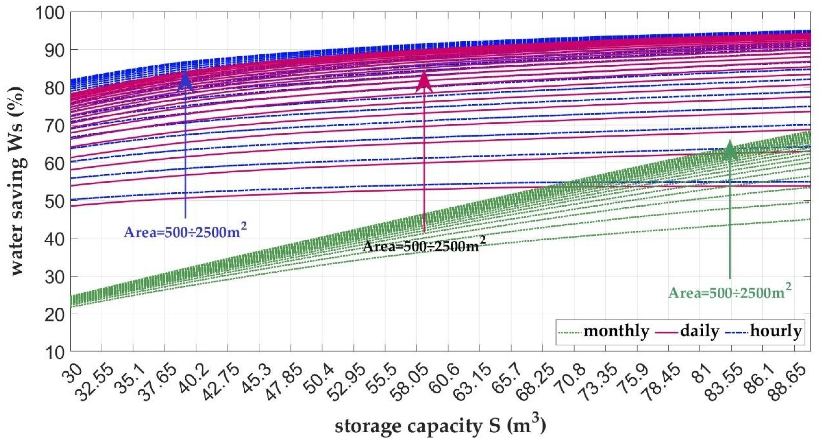
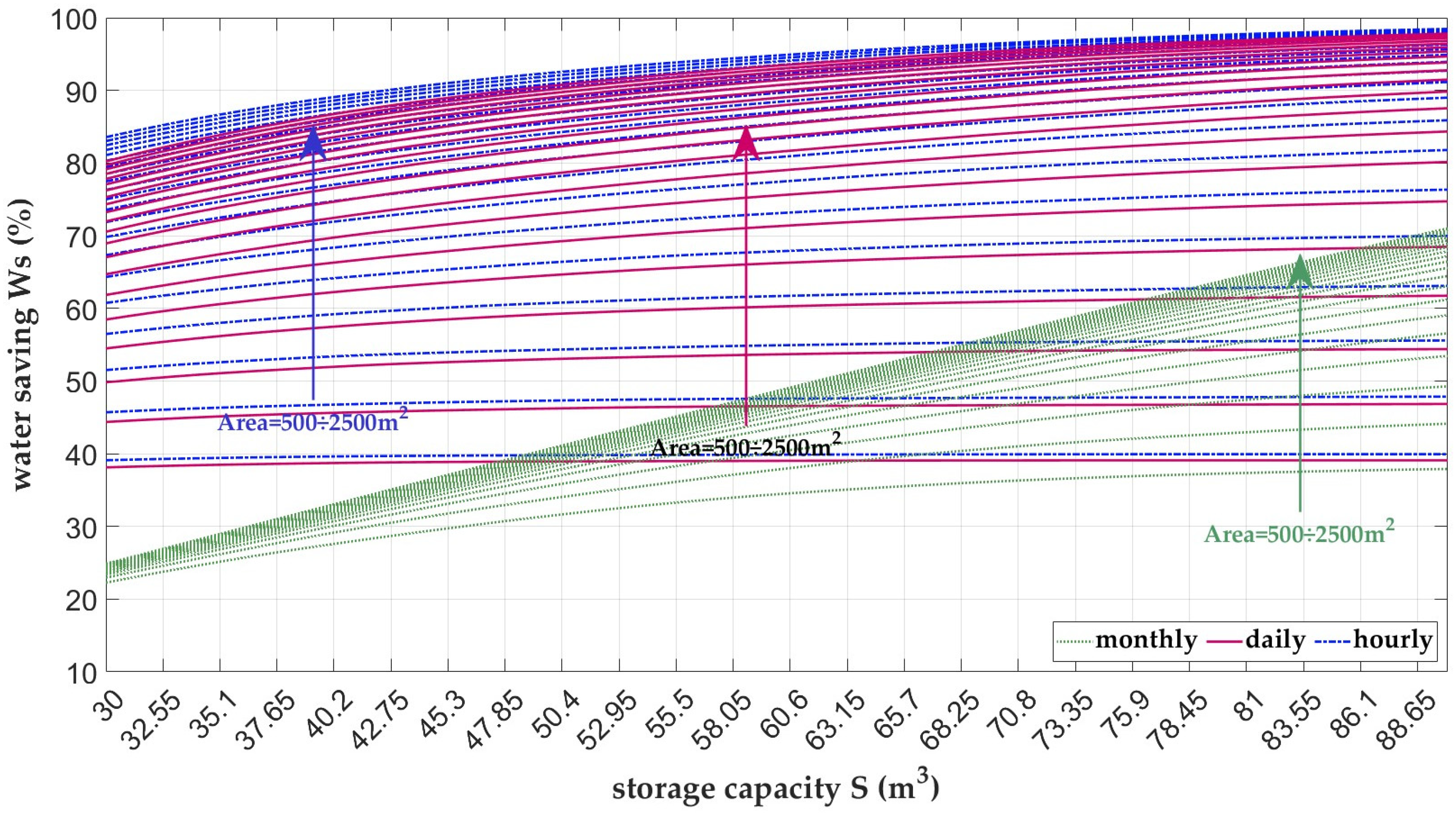
A comparative analysis of the simulation results is presented in Figure 6 for Lazio and Figure 7 for Denmark. Each figure illustrates variations in water savings as a function of both storage capacity and rainwater collection area. The results are based on simulations using three temporal resolutions—hourly, daily, and monthly—across 21 values for catchment area (A), ranging from 500 m² to 2500 m² in 100 m² increments, and 61 values for storage capacity (S), ranging from 30 m³ to 90 m³ in 1 m³ increments.

The results indicate that simulations using a monthly time step consistently underestimate system performance. In contrast, outputs from the hourly and daily simulations closely align, validating the reliability of the daily resolution. Consequently, a daily time step will be used in subsequent analyses to balance model accuracy with computational efficiency.

4.3. Nomograms

The extensive results from 500-year simulations, carried out by using various combinations of storage capacity S and catchment area A, along with synthetically generated demand and precipitation time series, have been synthesized using three key ratios introduced in this study (Section 2.1) and which are widely recognized in the literature [7,9]: storage fraction $sf$, demand fraction $df$, and storage period $sp$. 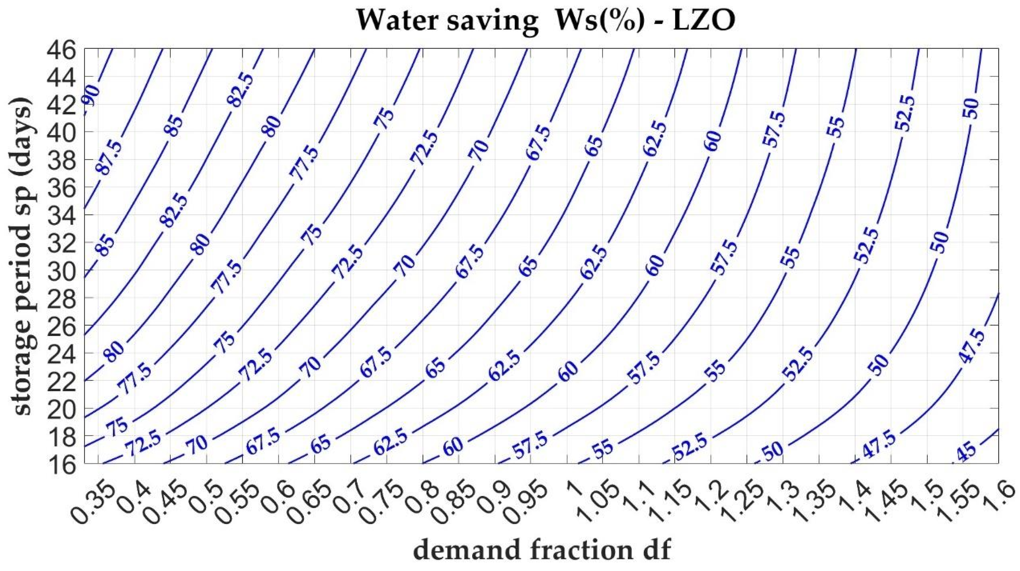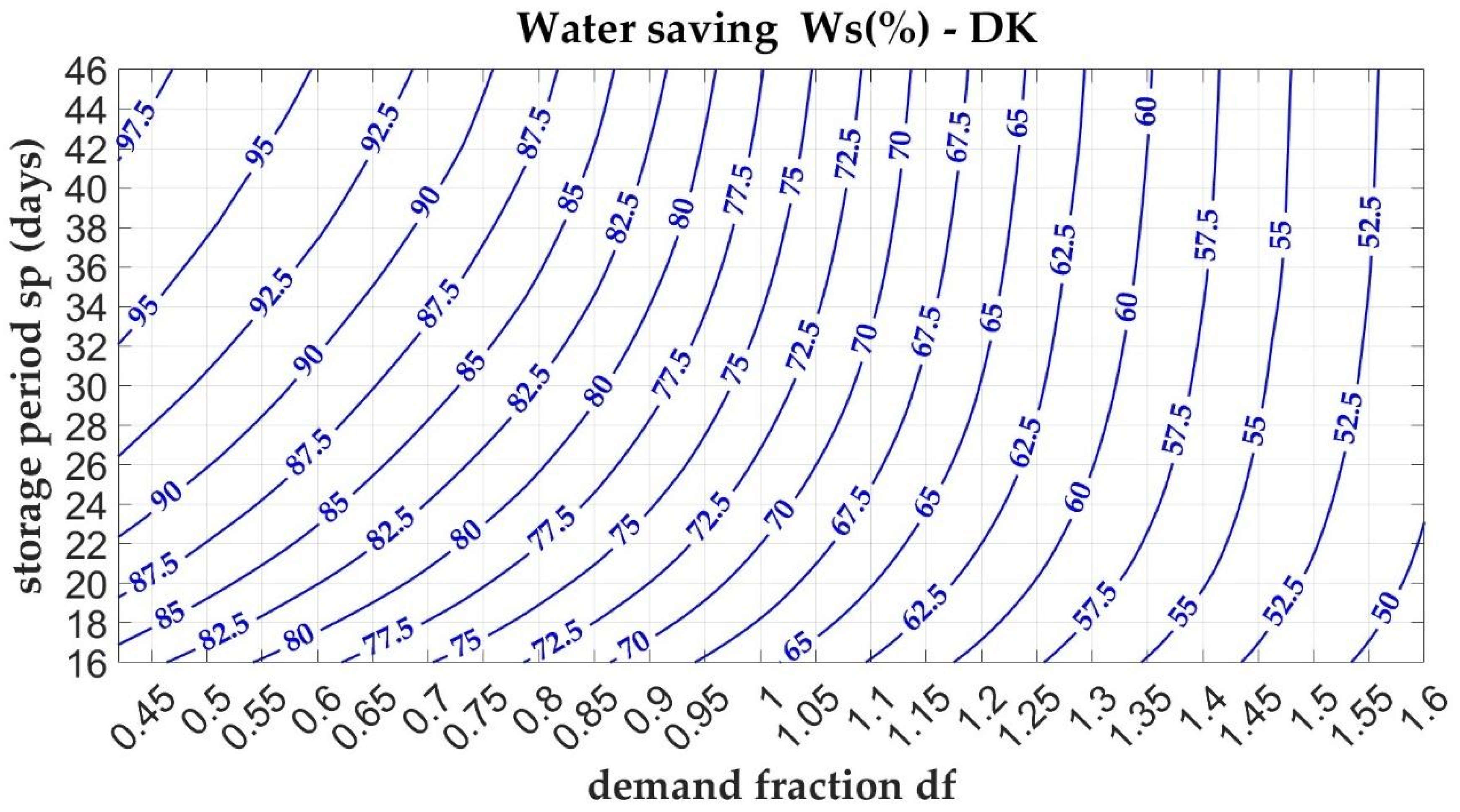For each of the four primary performance metrics of the rainwater harvesting (RWH) systems (Section 2.1), i.e., the water-saving efficiency ($W_S$), mean monthly savings ($M$), overflow discharge ($O_D$), and reliability ($Re$), nomograms can be derived. These graphical tools support system sizing by enabling users to identify suitable storage volumes and catchment areas corresponding to target values of the selected metric. Here, only the nomograms of the performance parameters $W_S$ and $Re$ are reported. 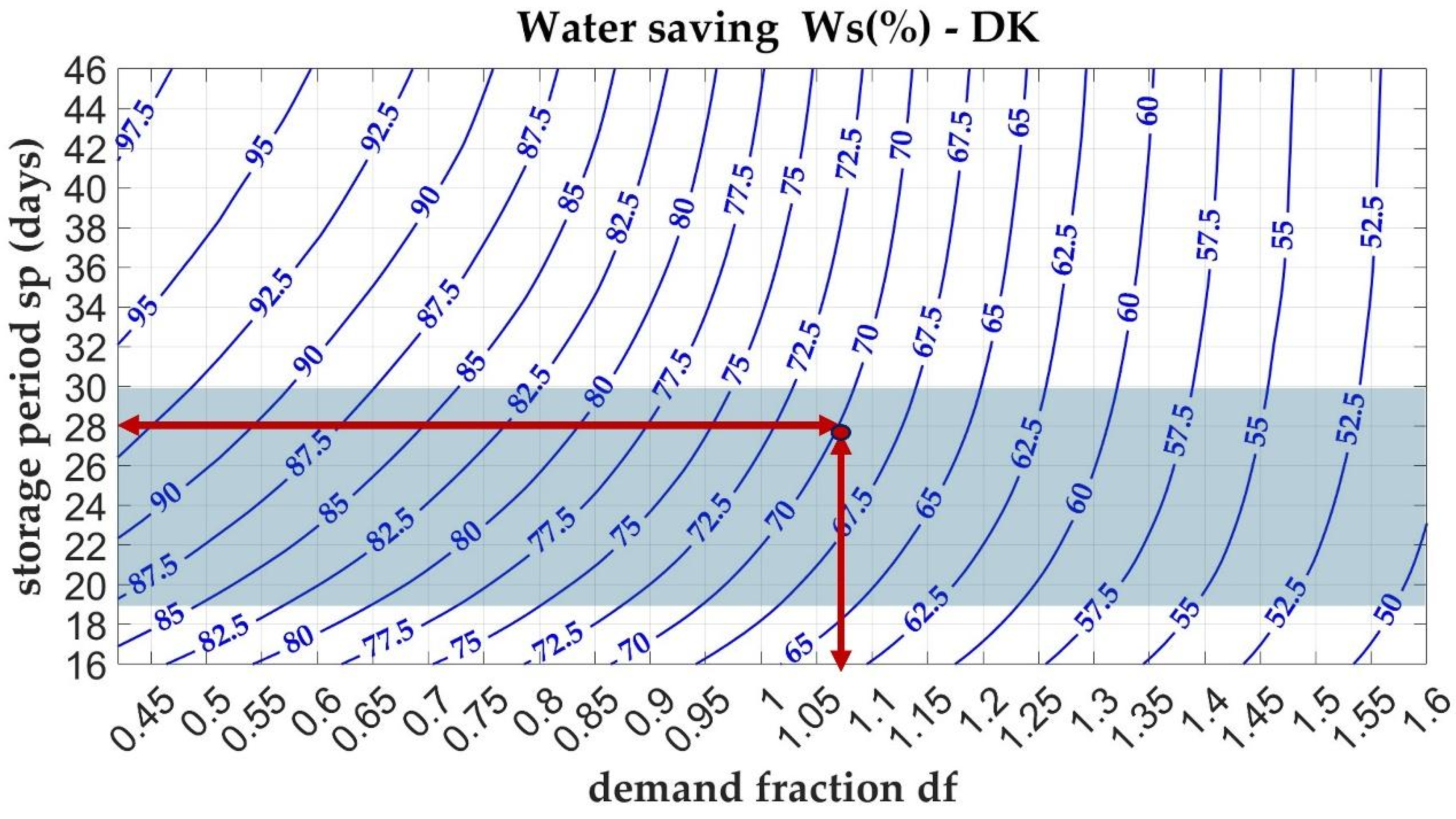Specifically, Figure 8 and Figure 9 display the nomograms for the water-saving efficiency parameter ($W_S$) for the Lazio (central Italy) and Denmark case studies, respectively. 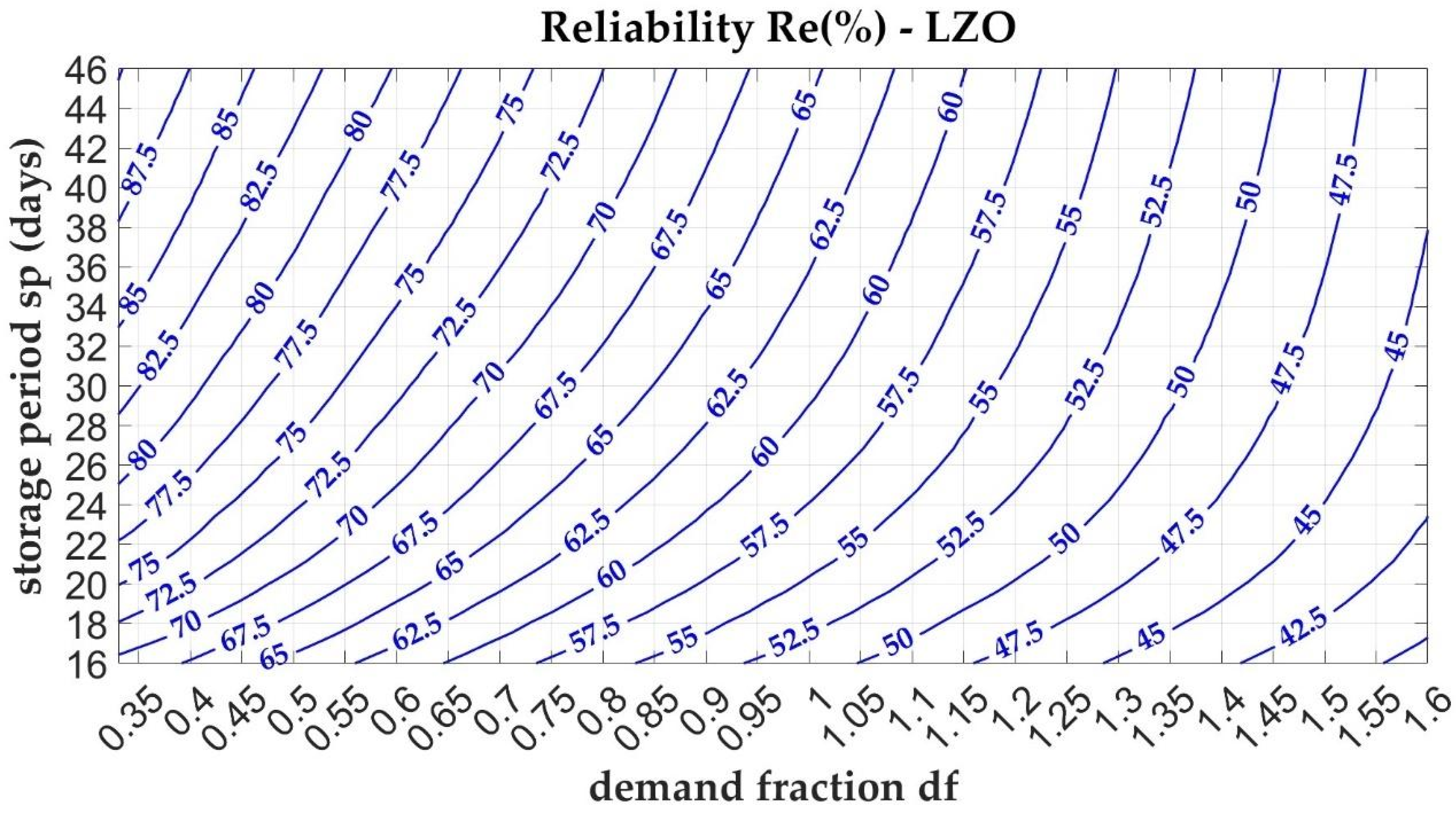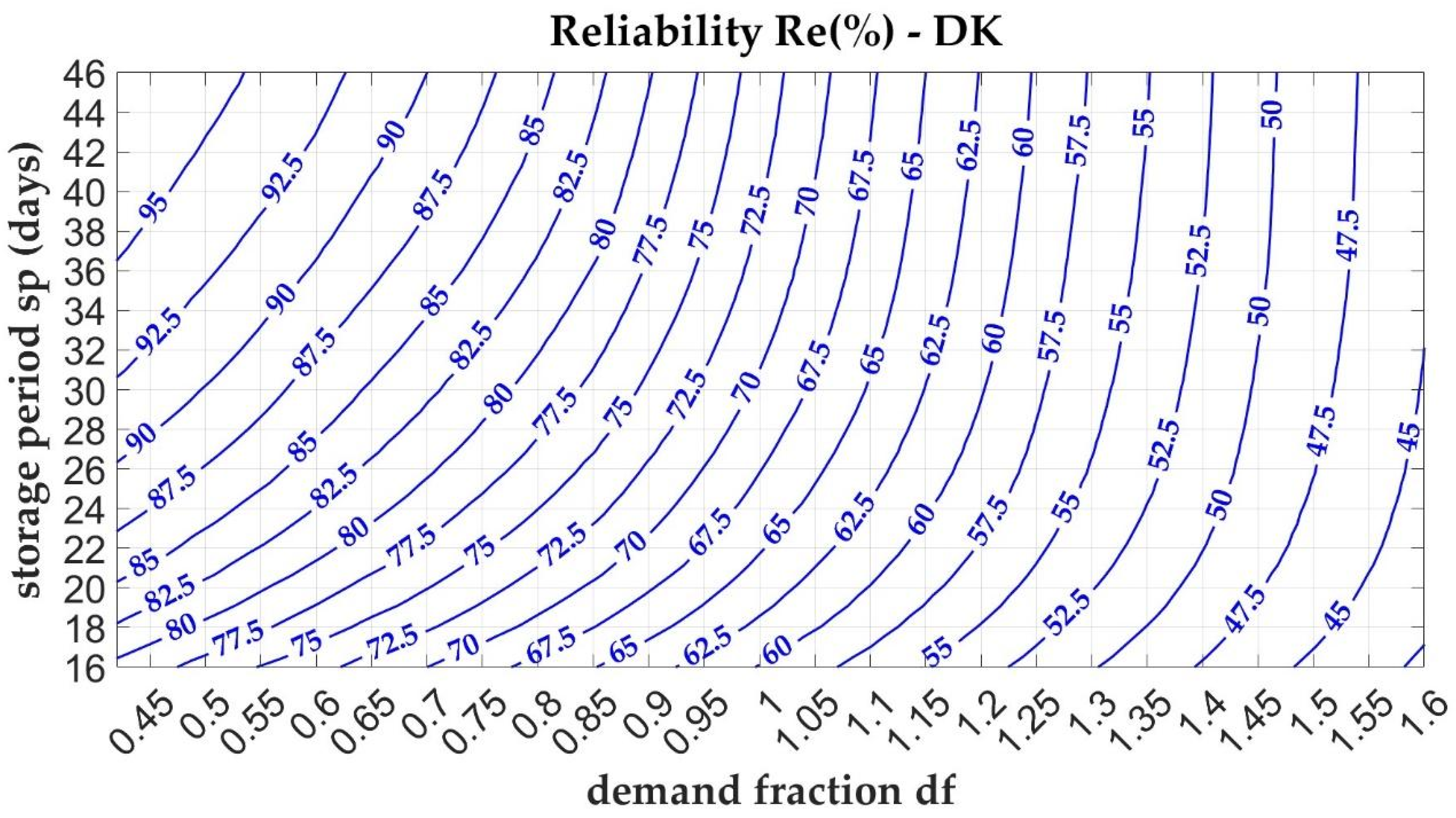Figure 10 and Figure 11 present the corresponding nomograms for the reliability parameter ($Re$). In each graph, solid curves illustrate the relationship between the respective parameter ($W_S$ or $Re$) and two key variables: the demand fraction $df$(dimensionless) and the storage period $sp$ (expressed as a time measure).

Along the horizontal axis, the demand fraction $df$ increases, reaching values greater than one ($df$ > 1), which correspond to scenarios where water demand exceeds the available collected volume. This imbalance can result from either excessive water demand or insufficient water collection, typically due to low rainfall or a small catchment area. As the $df$ ratio increases, the water savings $W_S$ provided by the storage tank diminish. Conversely, reducing the $df$ ratio, either by expanding the effective catchment area or decreasing water demand, enhances the water saving performance. At the same $df$ level, the Danish case study exhibits a higher $W_S$ compared to other cases. Furthermore, in the Danish context, $W_S$ shows a noticeably lower sensitivity to variations in the storage period $sp$, indicating more consistent performance across different storage durations.

The vertical axis represents the storage period $sp$ that can be interpreted as the emptying time, i.e., the tank volume to average water demand ratio. For a fixed demand, sp increases with tank volume. $W_S$ improves with longer emptying times $sp$ and lower values of the demand fraction $df$. The behaviour of the $Re$ performance parameter parallels that of $W_S$: it increases with greater storage durations (i.e., higher $sp$) and decreases with higher $df$. In the Danish case study, for a given $df$, $Re$ values are generally higher and less sensitive to variations in storage duration.

The nomogram should be used with the understanding that the emptying time $sp$ can be assumed either as the reference dry period (DP), defined as specified percentile of the waiting time between two consecutive rainfall events (Section 4.1), or as the maximum allowable storage duration (SD) for water in the tank, following similar parameters defined in the technical standards. In fact, from a design optimization standpoint, the tank volume should be able to meet water demand for at least the duration of the reference dry period in the absence of rainfall. But, due to reasons related to water quality, it should not remain in the tank for too long.

In summary, the following inputs are required to utilize the nomogram:

• $\tilde{I}$: Average daily rainfall intensity;
• DP: Reference duration of dry periods;
• $\tilde{D}:$ Average daily water demand;
• SD: Maximum allowable storage duration;
• W_S, M, O_D, Re: Target efficiency/reliability parameter.

The procedure can follow two alternative approaches, explained below.

First approach:

(a)

Selection of an emptying time (sp) value: Choose an emptying time (sp) that lies between the reference dry period (DP) and the maximum allowable storage duration (SD).

(b)

Computation of the storage capacity (S): Calculate the storage volume (S) corresponding to the selected emptying time (sp) value.

(c)

Performance metric intersection: Identify the point where the selected emptying time (sp) intersects with the target value for the desired performance metric, ensuring alignment with the system’s operational goals.

(d)

Determination of the required catchment area (A): Using the demand fraction (df) corresponding to the intersection point in step c, compute the required catchment area (A) necessary to achieve the desired performance outcomes.

Second approach:

(a)

Selection of collecting area: Identify a catchment area (A) that aligns with the established design.

(b)

Computation of demand fraction (df): Calculate the corresponding demand fraction (df) based on the selected catchment area.

(c)

Performance metric intersection: Determine the intersection point where the computed demand fraction (df) aligns with the target value for the chosen performance metric.

(d)

Determination of the required storage capacity (S): Using the storage period (sp) derived from the intersection point in step c, compute the necessary storage volume to meet the desired performance outcomes. Ensure that the storage period (sp) falls between the reference dry period (DP) and the storage duration (SD), balancing both constraints to optimize system performance.

In the first approach, different catchment areas are obtained for the same storage volume depending on the performance metric. In the second approach, different storage volumes are obtained for the same catchment area and performance metric.

To evaluate whether the rate of change in area (first case) or volume (second case) is affected by climatic conditions (e.g., Lazio vs. Denmark), a numerical example is provided for both case studies, considering the performance parameter Ws.

4.4. Numerical Example

For both case studies, a daily average flow rate of 1.9 m³/day for toilet flushing is assumed. As previously detailed, this corresponds to the water consumption of 10 households, each comprising an average of three inhabitants. The average annual rainfall is estimated at 898.1 mm for Lazio and 614.7 mm for Denmark. The storage period, defined as the time required to empty the storage tank, must lie between the reference dry period (DP) and the maximum permissible water retention time in the tank, as outlined in Section 4.3. The maximum storage duration is assumed to be the same for both regions, set at 30 days. Conversely, the reference dry period, derived from the rainfall time series presented in Section 4.1, is assumed as 27 days for Lazio and 20 days for Denmark. This indicates that the likelihood of dry periods is lower in Denmark, as also shown in Figure 5. Consequently, in the Danish case, there is a higher probability of selecting a favourable initial storage period (sp) value.

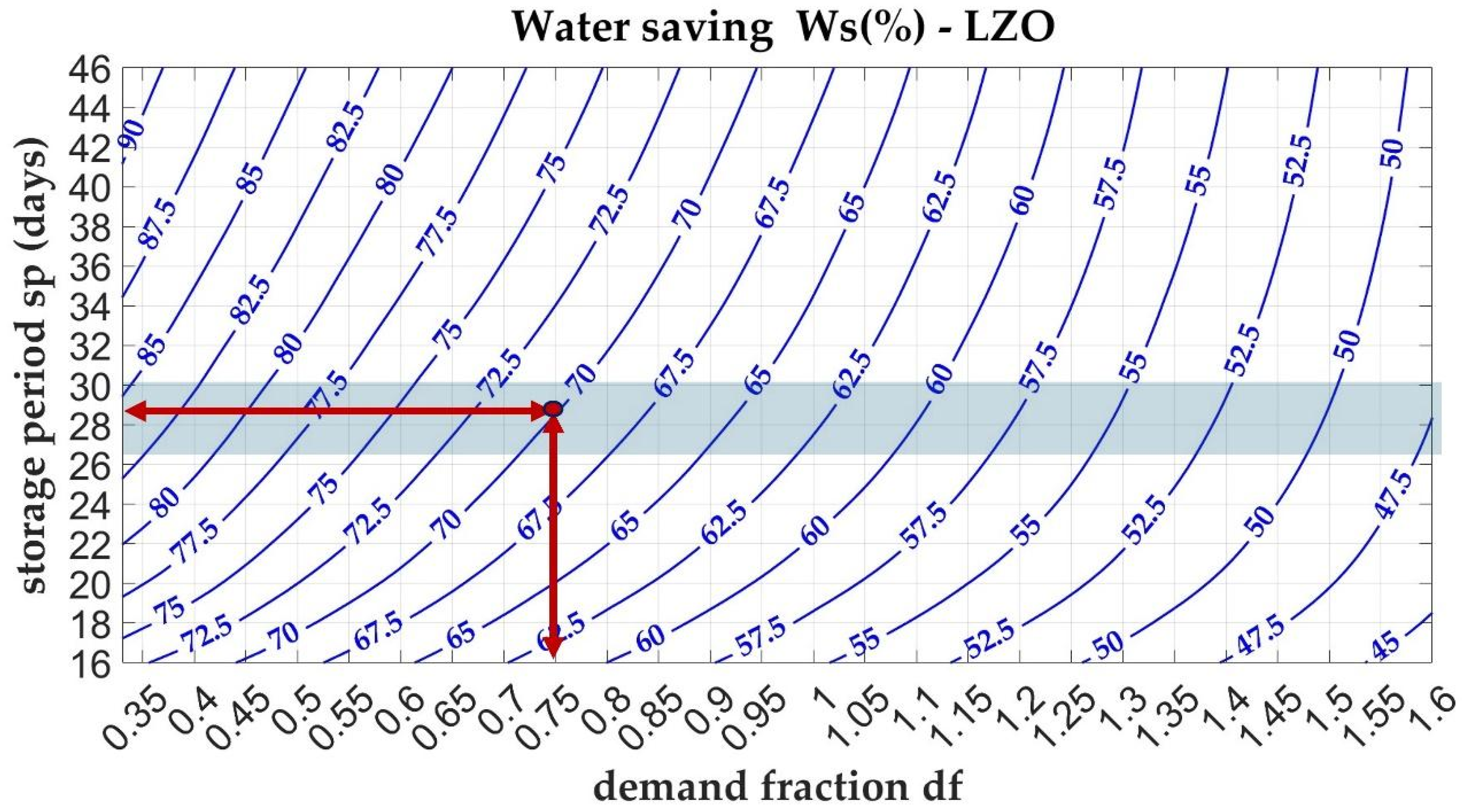
Following the first approach in the use of the nomogram (Figure 12 and Figure 13), a storage period of 28 days is selected, which is suitable for both case studies. Based on this value, the required tank volume is determined to be 53.2 m³ for both cases. By setting the design objective to achieve a performance index $W_S$ = 70%, the resulting demand fraction for the Lazio case is $df$ = 0.75, corresponding to a required catchment area A of about 318.31 m². For the Danish case, the demand fraction is $df$ = 1.07, which corresponds to a catchment area A of about 396.16 m². Alternatively, by selecting the minimum emptying times, 27 days for Lazio and 20 days for Denmark, a storage volume of S = 51.3 m³ would be required for a collection area of A = 305.6 m² in the former case, while a volume of S = 38 m³ would suffice for an area of A = 507 m² in the latter.

If the design constraints impose a maximum allowable collection area, the nomogram can be applied using the second approach. Let us assume a catchment area A = 1000 m². Based on this value, the corresponding demand factors $df$ are approximately 0.81 for Lazio and 1.0 for Denmark. Using these demand factors, the required tank volume for Lazio can range between 49.4 m³ and 57.0 m³, resulting in a performance index $W_S$ between 67.5% and 69%, consistently below the 70% threshold. In contrast, for Denmark, the storage volume may vary between 38.0 m³ and 57.0 m³, yielding a performance index between 68% and 74%.

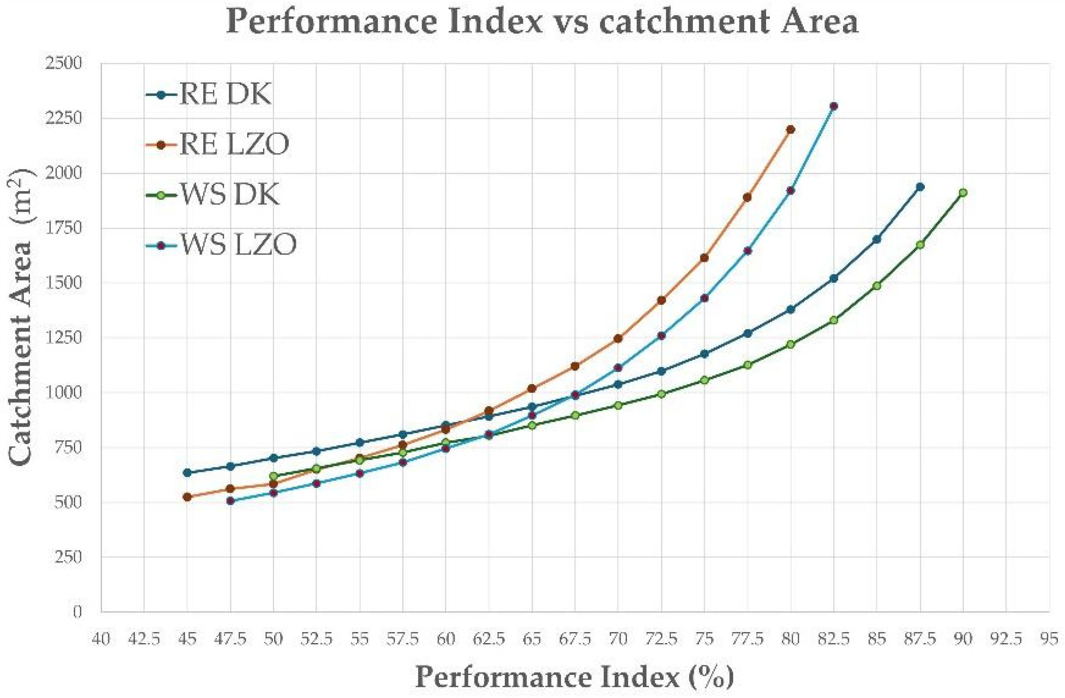
Following the second method of nomogram analysis, Figure 14 illustrates the catchment area corresponding to various values of the performance indices (Ws and Re) for a fixed storage period sp = 27 days, which implies a constant storage volume. It can be observed that, for performance index values exceeding 60%, both curves representing the Lazio region (Italy) exhibit higher area values (A) compared to the Danish case. For lower performance index values, the behaviour of both case studies appears similar.

5. Conclusions

This study proposes a comprehensive, simulation-based methodology for the design of rainwater harvesting (RWH) systems in residential settings, integrating the stochastic modelling of both precipitation and water demand. By employing a behavioural model—specifically the Yield After Spillage (YAS) algorithm—this work enables the derivation of performance-based nomograms that support the simultaneous and flexible determination of storage volumes and catchment areas. The methodology is designed to achieve predefined thresholds of efficiency and reliability while accounting for local climatic characteristics. Notably, the analysis across two climatically contrasting regions, Lazio (central Italy) and Denmark, demonstrates the method’s adaptability and highlights the significant role played by local rainfall dynamics and dry period characteristics in influencing system performance. The dimensionless parameters introduced, such as demand fraction and storage period, allow for the generalization of the results and comparative assessments across case studies. Moreover, the results confirm that higher temporal resolutions (e.g., daily over monthly) lead to more accurate performance evaluations, although the marginal gains must be weighed against computational effort. The nomogram-based approach offers both flexibility and clarity for practitioners, enabling tailored system design based on available space, water demand, and climatic constraints. Future developments will include the following:

• Definition of ad hoc nomograms for other different climatic zones and other water demand schemes (by also including gardening or other residential uses, such as showering or laundry). Specifically for rainfall input, any other climatic pattern can be easily reproduced by modifying the parameter values of the stochastic rainfall generator.
• Making the model a predictive methodology, i.e., by taking into account the possible effects of climate change on the rainfall input, which is mainly useful for synthetic time series with a size greater than 30 years.
• Quantifying the parameter uncertainty and analyzing its effects. This is mainly important when summary statistics (used for the calibration of the considered input stochastic models PRP and NSRP) are estimated from observed series with a small sample size (e.g., less than 10–15 years).

Overall, the proposed framework stands as a practical, scalable tool that aligns with sustainable water management goals and supports the widespread implementation of RWH systems in urban and peri-urban contexts.