1. Introduction
Recently, reducing greenhouse gas emissions has become a major focus in automotive and transportation research. According to estimates by the Environmental Protection Agency, the transportation sector was responsible for 28% of total greenhouse gas emissions in the United States in 2022, making it the largest single contributor [
1]. Therefore, improving the energy efficiency of vehicles has emerged as a key strategy for reducing transportation-related emissions. One promising approach to enhancing passenger vehicle energy efficiency involves developing connected and automated vehicles (CAVs). Unlike human operators, CAVs can process a much larger dataset in real time without suffering from distraction or fatigue, thereby offering significant potential for increasing energy efficiency.
This study introduces a novel approach to improving passenger vehicle energy efficiency by automating route selection using the capabilities of CAVs. Traditional routing algorithms typically focus on distance, travel time, or ease of navigation for human operators. Taking a route with a similar travel time but a shorter distance than another route may lead to significant fuel savings [
2]. However, this is not always the case, as factors such as speed, acceleration, and the number of stops also have significant impacts on fuel consumption [
3]. Therefore, while shorter routes are generally more efficient, they do not always guarantee optimal energy usage. Our findings demonstrate that routes selected by an autonomous agent can achieve better energy efficiency than those chosen solely based on the shortest distance or travel time.
The development of an autonomous routing agent requires integrating a traffic network simulation software package, a vehicle model, and an optimization algorithm. In this study, the Simulation of Urban MObility (SUMO) traffic simulator, a widely-used tool for constructing and testing traffic networks, is employed [
4]. SUMO interfaces with both an internal vehicle model and an optimizing agent via the Traffic Control Interface (TraCI) Python module (version 1.3.1) in this study.
Recent studies show the growing importance of machine learning (ML) methods in advancing transportation sustainability. In particular, deep reinforcement learning (DRL) has shown considerable promise in intelligent routing, vehicle control, and adaptive traffic signal optimization. ML-driven decision making frameworks enable real-time adaptation to dynamic environments, offering a significant advantage over traditional rule-based or heuristic methods [
5]. The routing algorithm employed in this study is a modified version of AlphaGo Zero, which is a model-based deep reinforcement learning (MB-DRL) algorithm originally designed to play board games at a superhuman level [
6].
Recent advancements in MB-DRL algorithms, exemplified by AlphaGo Zero, have shown great potential in providing near-optimal solutions for complex systems with large state and control spaces. AlphaGo Zero learns to optimize the game of Go by constructing a decision tree that operates in conjunction with a deep residual neural network (ResNet). The decision tree and ResNet recommend moves with a high probability of leading to a victory in the game. The decision tree models the game dynamics, provides move recommendations at each node, and calculates a final score for the game. Concurrently, the ResNet predicts the final score for each node explored and estimates the probability of selecting legal moves from a parent node to its children. These predictions and estimates from the ResNet are then backpropagated through the decision tree to update the decision tree parameters. The differences between the ResNet’s final score predictions and the actual scores of the decision tree are calculated, as well as the differences between the ResNet’s move predictions and the decision tree’s move recommendations. These two difference calculations are combined to form the loss function that optimizes the learning parameters of the ResNet. The result is a self-improving algorithm that simulates games of Go, with the decision tree and ResNet collaboratively refining strategies for optimal moves. No human knowledge is required to find the optimal moves, and thus the algorithm is not limited by human-level performance. AlphaGo Zero has notably outperformed its predecessor, AlphaGo, with a record of 100 victories to 0 in their matchups. As a point of comparison, AlphaGo had previously defeated the human world champion in four out of five matches. In this work, the authors make the first successful attempt to use a modified version of AlphaGo Zero to find the optimal routes for a passenger vehicle with respect to energy efficiency.
2. Related Research
Several studies have been conducted to increase fuel efficiency with varying degrees of autonomy and vehicle connectivity. One approach focuses on increasing traffic throughput as a means of improving the network-level fuel efficiency [
7,
8]. While effective, increasing the throughput alone does not consider vehicle powertrain efficiencies, the impact of improved traffic flow in one area on the wider traffic network, or the benefits of taking alternative routes for some vehicles. Including these factors should provide opportunities for further improvement.
One such alternative approach that includes a powertrain model is eco-routing, where efficient routes are determined based on the average energy cost to traverse each road segment [
9,
10,
11,
12,
13]. Eco-routing has been previously achieved using several methods. For example, a brute force method has been studied for a single vehicle in a traffic network [
14]. Although this method provides efficient routes under varying traffic signal conditions, congestion, which is a significant contributor to the network-level energy consumption, is not considered. Another eco-routing method utilizes GPS data obtained from connected vehicles, which inherently accounts for congestion [
15]. However, the routing scheme is not dependent on real-time traffic signal timing, which contributes significantly to the energy consumption of any selected route. A stochastic model has also been implemented to allow for variability in the edge eco-weights at different times of day [
16]. Eco-weights are the average energy cost for each road or road segment. This method offers a higher level of flexibility but still lacks the traffic signal timing for each intersection. Knowledge of the traffic timing in the network through vehicle connectivity could reduce the number of stops, which may have a significant impact on the efficiency of a route.
In addition to these methods, global optimization methods have been applied to fuel-efficient routing. Dynamic programming (DP) can find an optimal solution for a system of any size and complexity, given enough computational capacity, whether the system is deterministic, stochastic, or a combination of both. DP has been implemented to find the optimal routes with respect to fuel efficiency for individual vehicles in traffic networks [
17,
18,
19,
20]. DP guarantees an optimal solution, but only if full knowledge of the dynamics for the remainder of the driving episode is provided to the algorithm. This includes knowing the position of every vehicle in the network for the duration of the trip before optimization begins. This is not possible for a realistic traffic scenario, where all or most vehicles are driven in an unpredictable manner. In addition, given that the DP solution for one vehicle is computed to the order of seconds, it is a computationally expensive approach if the entire traffic network should be considered. For this reason, calculating the global optimal solution for city-scale traffic networks with multiple vehicles using DP is not feasible.
Although DP and heuristic eco-routing can achieve comparable energy efficiency with greater transparency and interpretability, both have significant drawbacks. DP requires a complete Markov model, which limits its scalability to large traffic networks. Heuristic eco-routing offers better computational efficiency than both DP and the proposed method; however, it relies heavily on expert-crafted rules that may not generalize well across different networks. In contrast, the proposed AlphaGo Zero-inspired DRL approach learns optimal routing policies without requiring prior domain knowledge. While this comes at the expense of some interpretability, DRL enables the discovery of novel traffic management strategies that traditional methods may overlook. DRL is a branch of machine learning that uses deep neural networks to find near-optimal solutions to complex systems, ranging from video and board games to mobile robot navigation [
21,
22,
23,
24]. While DP explores all allowed actions in each system state, DRL algorithms estimate the actions that are most likely to produce desirable results. Also, while DP and other optimal solution methods require complete knowledge of the system, DRL algorithms discover abstract features of the system autonomously. Although DRL does not guarantee global optimal solutions, the solutions are calculated to the order of milliseconds after training on a desktop computer.
Combining DRL and CAVs has provided promising results in optimizing the fuel efficiency of individual vehicle powertrains in simplified traffic networks [
25,
26]. These works utilize Deep Q-Learning, a family of model-free DRL algorithms that estimate the value of state-action pairs for a given environment. Although possessing many advantages of DRL, Deep Q-Learning is limited by the discrete state space and control space. A more complete solution to the traffic network-level fuel efficiency optimization problem requires an algorithm that can explore much larger state and control spaces than Deep Q-Learning for the same computational power. One study showed that a Deep Deterministic Policy Gradient (DDPG) algorithm can resolve this issue by employing the actor-critic approach [
27]. As another model-free DRL method, DDPG is particularly suited for solving problems with continuous action spaces but also tends to be inefficient with respect to the sample count.
To address the issue of the low sampling efficiency of model-free DRL algorithms, this study utilizes a model-based method that incorporates an environment model with a discrete action space. Knowledge of the environment model allows for more efficient exploration by focusing on promising states and avoiding those known to yield poor outcomes. This is achieved by analyzing and learning from optimal sample sequences instead of evaluating each sample in isolation. Additionally, the model-based methods’ ability to learn from sequences of samples enhances their capability to generalize to new, unseen states, which is an advantage over model-free algorithms. This aspect of sample efficiency and generalization is particularly important in optimizing traffic networks, as generating all possible states in each traffic network is prohibitively expensive, and traffic data tends to be difficult to acquire. An effective optimization method for traffic networks should be able to find a solution with a limited dataset and handle states never encountered during the training process. This research demonstrates that model-based deep reinforcement learning effectively meets these requirements.
3. Simulation Environment
3.1. Traffic Network Simulation Environment
For this study, a traffic network with a controlled vehicle was simulated in Simulation of Urban MObility (SUMO) software (version 1.3.1). SUMO is a powerful open-source tool for simulating urban traffic without the logistical and financial constraints of real-world experimentation. However, it has inherent limitations in replicating the dynamic and unpredictable nature of real-world traffic conditions. For example, it may not fully capture the complexities of human driving behavior, including spontaneous decisions and reactions to unforeseen events, or the varied impacts of environmental factors such as weather and road surface conditions. Despite these limitations, SUMO remains an invaluable tool for traffic simulation, offering significant advantages in terms of flexibility, scalability, and the ability to model a broad range of traffic scenarios and policies. For these reasons, numerous researchers and urban planners use SUMO to analyze traffic behavior, evaluate the impact of various transportation policies, and plan infrastructure developments before implementing them in the real world [
28,
29].
While SUMO provides a flexible and scalable platform for simulating traffic scenarios, it does not explicitly model stochastic state transitions or phase transitions in traffic flow. Real-world traffic exhibits emergent behaviors such as abrupt transitions from free flow to congestion due to small perturbations [
30,
31]. These effects are described in macroscopic traffic flow theory. In the current simulation set-up, vehicle behavior was deterministic once initialized, and signal timing remained fixed across all scenarios. Although some variability was introduced through randomized vehicle routes and departure times, these simplifications limited the model’s ability to fully capture dynamic phenomena such as congestion shockwaves or spillback effects. To address this limitation, future work will incorporate stochastic traffic models and variable signal timing plans to better reflect real-world uncertainty and phase behavior. This enhancement will enable more robust training and evaluation of reinforcement learning agents under conditions that more accurately mirror operational traffic systems.
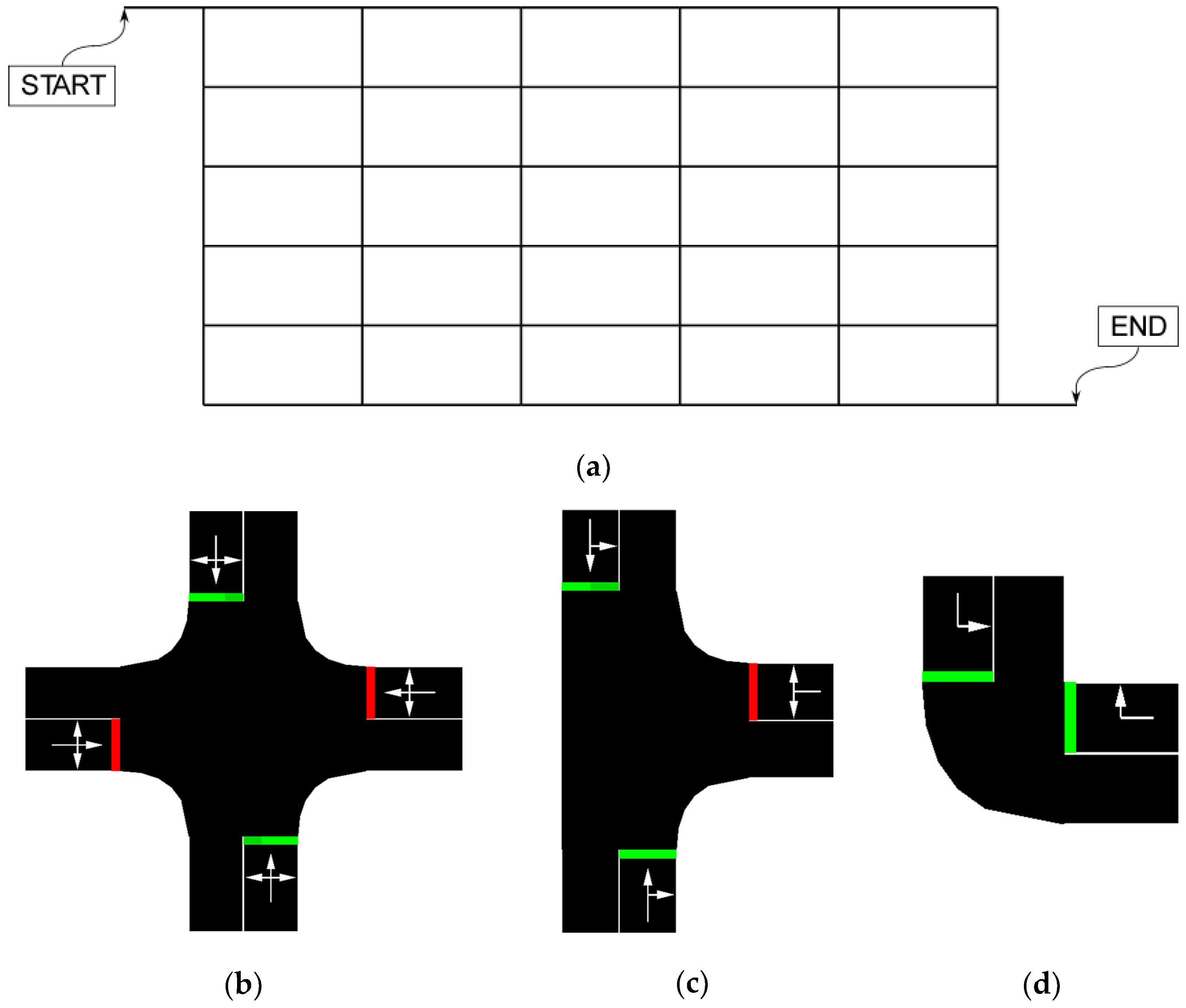
The studied network consisted of 36 intersections arranged in a rectangular grid, with six roads running longitudinally and six roads running laterally, as shown in
Figure 1a. Two additional road segments represented the start and end points of the controlled vehicle as labeled in the figure. Each road segment in the network contained two lanes, with one for each direction of travel. The east-west road segments were 200 m in length, and the north-south road segments were 100 m in length. This is similar to the standard grid size for residential streets in the city of Chicago and other major cities in North America. Additionally, the start and end road segments were 100 m each in length. This simple traffic network serves as an effective platform for the proof of concept in this study. Depending on the location, three different types of intersections were formed in the network, as shown in
Figure 1b–d.
Traffic signals controlled each intersection in the network. A detailed description of each traffic signal program used in the simulation is shown in
Table 1. In the network, the traffic signals in both the uppermost and lowermost horizontal rows were controlled by Program 1, those in the second and fifth rows were controlled by Program 2, and those in the middle two rows were controlled by Program 3.
During the simulation, a total of 50 vehicles were used to represent the traffic load. Each vehicle originated at the beginning of a random road and had a random destination road. The beginning of a road was defined as the furthest point from the next intersection along the direction of travel. Vehicles were removed from the simulation when they completed driving across the full length of the destination road in their routes. The routes for each vehicle were computed automatically using the SUMO routing function.
Each vehicle followed the rules defined by SUMO at the beginning of the simulation. The vehicle model used was based on SUMO’s default passenger vehicle. Each vehicle was 5.0 m long and weighed 1500 kg. A minimum gap of 2.5 m was maintained from the vehicle ahead, and the reaction time was set to 1.0 s. The maximum speed and acceleration were set to 55.55 m/s (124.4 mph) and 2.6 m/s2, respectively. The simulation ran for a maximum of 240 s, advancing in one-second time steps.
In addition to the 50 vehicles managed by SUMO, there was a special vehicle called the ego vehicle. The ego vehicle, typically an autonomous vehicle, serves as the primary test subject for validating the performance of new control strategies and behavior models in various simulated traffic environments. In this study, the route of the ego vehicle was optimized by the DRL algorithm as explained in
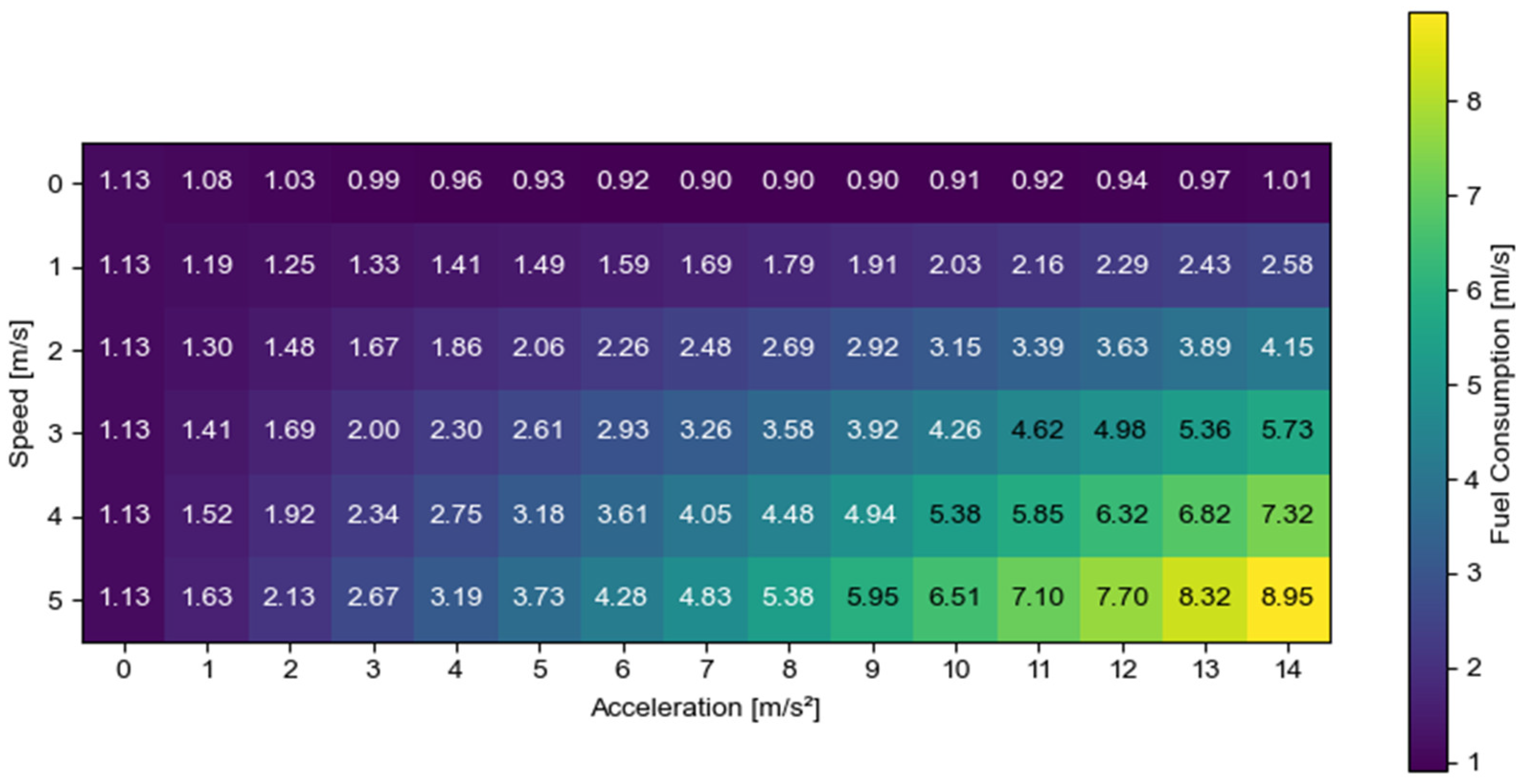
Section 4. All aspects of vehicle behavior, including fuel consumption, speed, acceleration, collision avoidance, and adherence to traffic signals, were handled by SUMO. This management encompassed the traffic load of 50 vehicles as well as the ego vehicle. An estimate of the fuel consumption of the ego vehicle was obtained at every simulation time step using the SUMO fuel efficiency model. This model is a tabularized estimate of fuel consumption based on the ego vehicle’s speed and acceleration, as shown in
Figure 2.
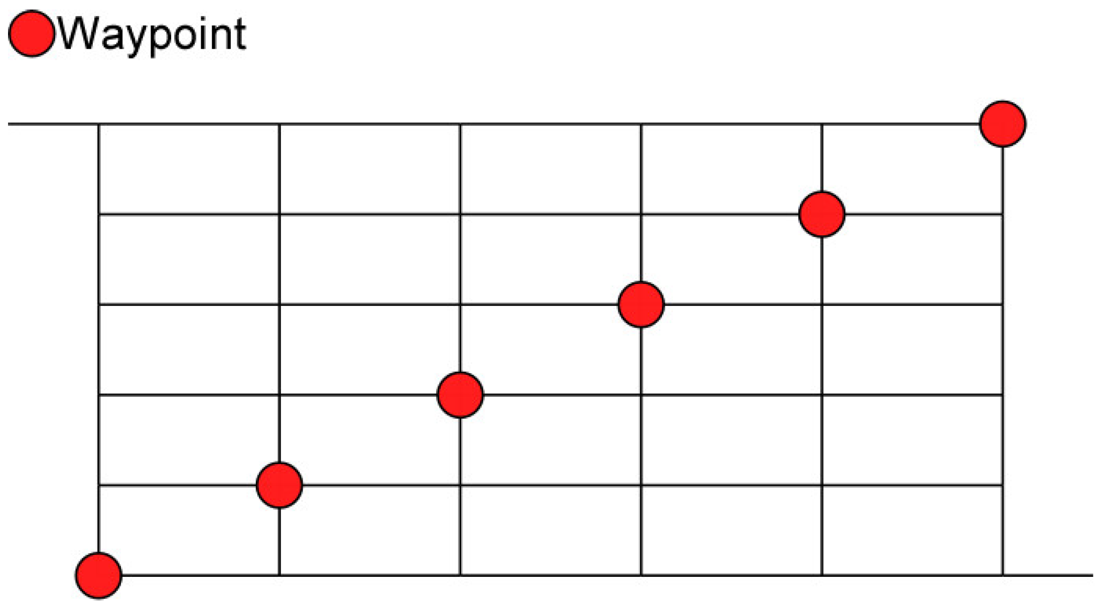
The route for the ego vehicle was constructed using a set of six user-defined waypoints placed along the major southwest-to-northeast diagonal of the traffic network, as shown in
Figure 3. Each waypoint was equidistant from the start point to the end point, both in terms of Cartesian distance and the number of road segments. This configuration encouraged the DRL algorithm to consider the impact of traffic signal states and congestion on fuel consumption, rather than simply opting for the shortest route. Additionally, each waypoint was positioned such that it could be reached from the start point without intersecting any other waypoint, thereby promoting exploration of the network. While other approaches may be possible, selecting routes based on a small set of predefined discrete waypoints provides a simple and consistent framework for evaluating different routes using interpretable, repeatable metrics. This structure also ensured manageable computational complexity, which is especially important in studying early-stage model-based reinforcement learning approaches. As explained in
Section 4, the DRL algorithm selects one of these waypoints, thereby making the action space discrete and mitigating the issue of low sampling efficiency. Once a waypoint is chosen, SUMO calculates the shortest path from the ego vehicle’s current location to this waypoint. SUMO also calculates a second route from the selected waypoint to the end point. These two routes are then merged into a single comprehensive path, which is assigned as the ego vehicle’s route. This route selection is the only control input that the learning agent provides to the ego vehicle.
3.2. Image Construction for Ego Vehicle and Traffic Network Data
To train the DRL algorithm effectively, both the ego vehicle data and other important traffic network data must be converted into a format suitable for the training process. In this study, the ego vehicle data and the SUMO simulation data were converted into grayscale images, with intensity values ranging from 0 (black) to 255 (white), as shown in
Figure 4. A two-dimensional image of 32 × 32 pixels was generated for each traffic network state defined by six state variables: the road layout, traffic load on each road segment, traffic light timings, location of the ego vehicle, route of the ego vehicle, and efficiency of the ego vehicle. To represent temporal variations in the traffic network state, the two-dimensional images were stacked to form three-dimensional images of 32 × 32 × 10 pixels. The third dimension of the images represents 10 sequential samples of the traffic state taken at 6-s intervals for a total of 60 s of traffic data. Including several sequential snapshots of traffic conditions facilitated the DRL agent to learn the dynamics of traffic flows, traffic light changes, and their combined effect on route efficiency. This multidimensional imaging approach provides a comprehensive view of the traffic system, which is essential for effective training of the DRL algorithm.
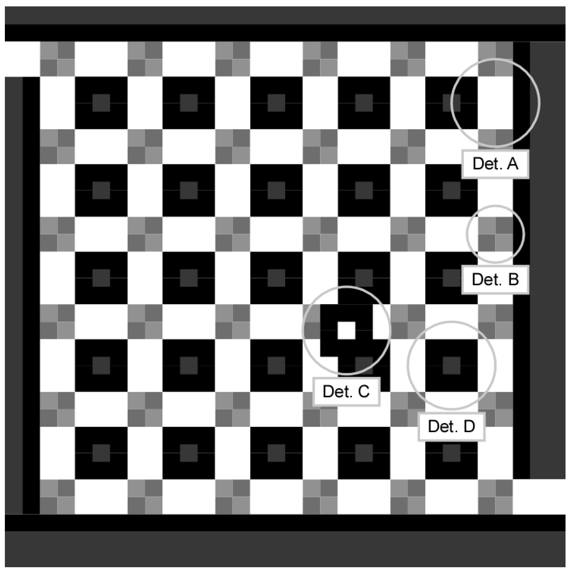
The state variables of the traffic network were represented by the geospatial image as shown in
Figure 5. However, this geospatial representation was not to scale, meaning that the length of each road segment in the image did not match the actual physical length of the corresponding road segment in the network. This is because a scaled geospatial representation would minimize the visibility of traffic loads and road locations in relation to the other state variables. This would diminish the ability of the DRL agent to learn the dynamics of the traffic network, which is a critical component in estimating the fuel efficiency of a given route.
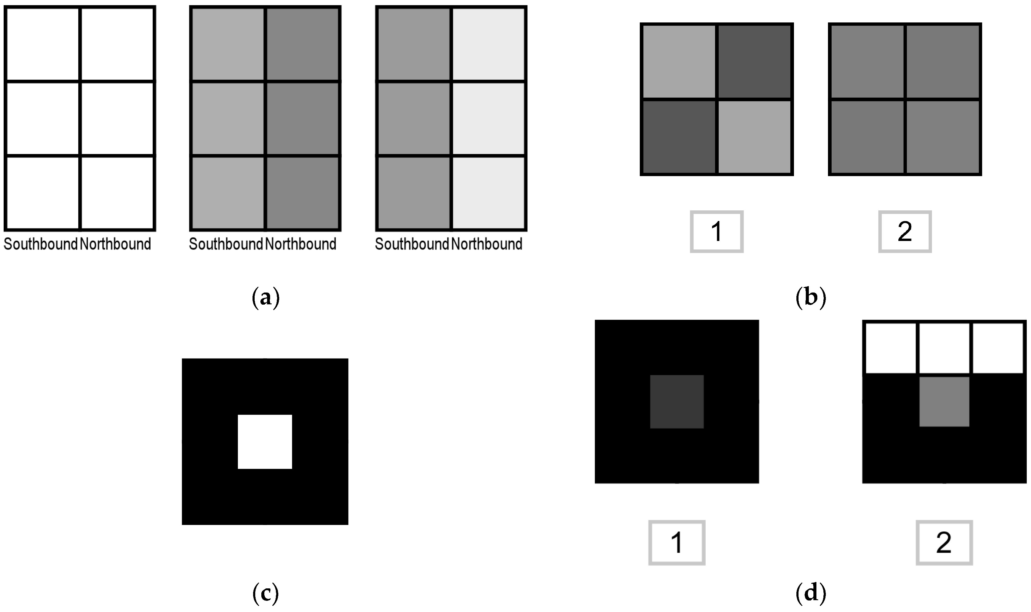
A road segment and its traffic load are denoted by a grayscale value of 135–255, with high traffic loads represented by low grayscale values. A maximum of 12 vehicles could be present on any given road segment, and each road segment in the image was two pixels wide to represent traffic loads for both travel directions (
Figure 6a).
The traffic light state with embedded timing information was also displayed using geospatial representation. Each of the 36 traffic lights is represented by a square area of 2 × 2 pixels in the 32 × 32 image layer, as shown in
Figure 5. The location of the light in the two-dimensional image layer corresponded to the physical location of the intersection controlled by the corresponding traffic light. The traffic light at each intersection controlled traffic flow in both the longitudinal (north-south) and lateral (east-west) directions. The upper right and lower left pixels in each traffic light square represent the lateral signal, while the upper left and lower right pixels in the traffic light square represent the longitudinal signal. Each of the four directional signals in each intersection was adjacent to the road segment controlled by the signal, maximizing the association between the dynamics of the road traffic and the state of the traffic light signal.
The grayscale values in the intersection area represent the traffic light signal timing information (
Figure 6b). A low grayscale value indicates a light that has recently turned red, while a high grayscale value represents a light that has recently turned green. This results in a high contrast within the intersection square whenever the traffic light phase has recently changed (
Figure 6b-1). On the other hand, as a traffic light nears a phase change, the grayscale value of the corresponding pixel gradually shifts toward a midpoint value of 127, leading to reduced contrast (
Figure 6b-2). Thus, both the pixel values and the contrast between the neighboring pixels provide information on both the current and upcoming states of each intersection. This set-up for the traffic light representation allows the DRL algorithm to learn the complex interplay between the signal states, intersection locations, and traffic flow dynamics.
For the ego vehicle location, a grayscale value of 255 (white) was assigned to the spatially associated pixel in the first two-dimensional layer. The pixel corresponding to the ego vehicle’s location was surrounded by a one-pixel border with a grayscale value of zero (
Figure 6c). The ego vehicle route is represented by the pixels adjacent to each road segment and travel direction. The default grayscale value for each set of pixels was zero (
Figure 6d-1), and the grayscale value was set to 255 if the associated road segment and travel direction were included in the selected route for the ego vehicle (
Figure 6d-2). The energy efficiency of the ego vehicle is represented in the image for all remaining pixels. One efficiency pixel was located at each center of the space between parallel roads (
Figure 6d-1). The remaining efficiency pixels were located along the outer borders of the entire image (
Figure 5). A high pixel value represents low energy efficiency, and a low value represents high energy efficiency.
4. Model-Based Deep Reinforcement Learning Algorithm
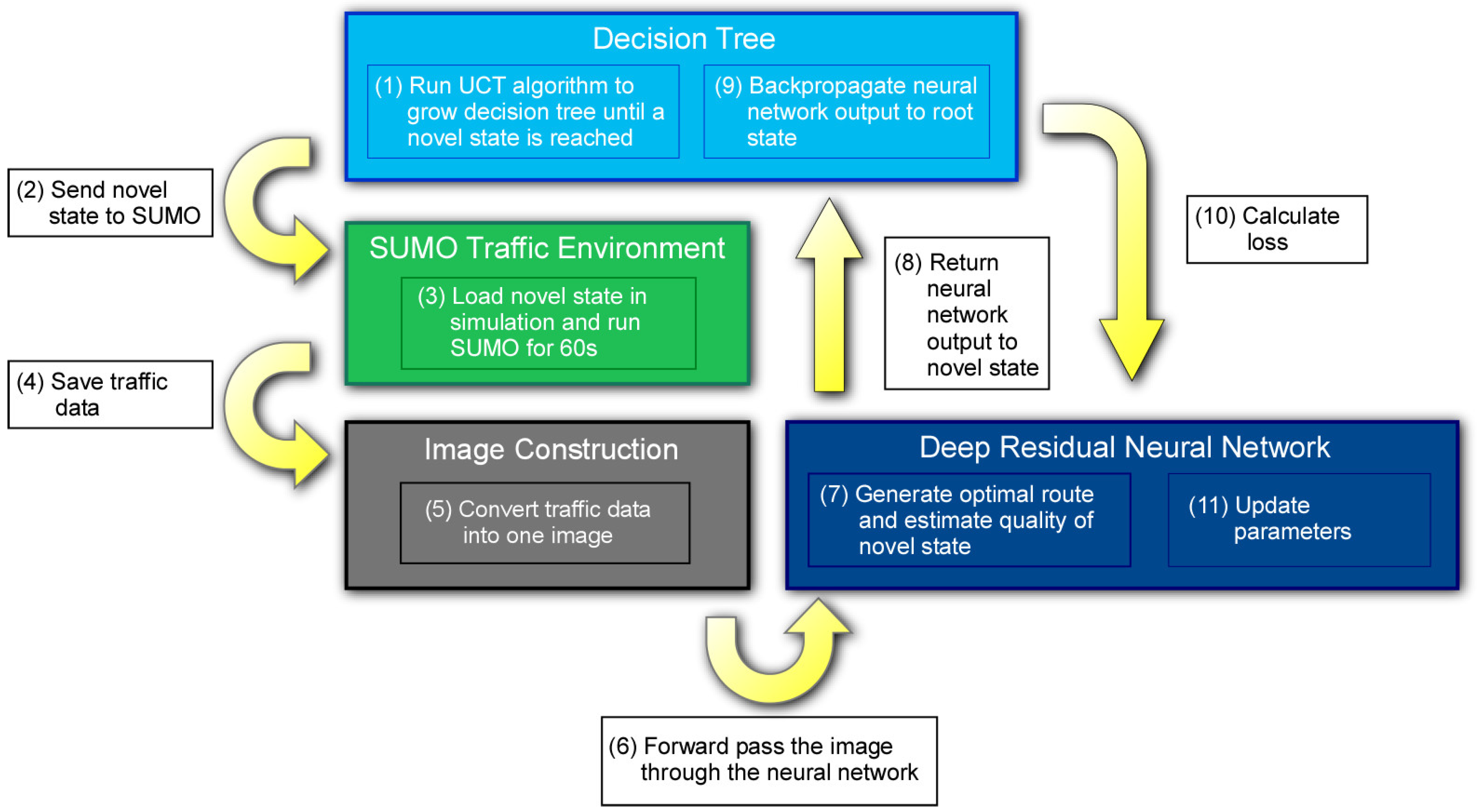
The model-based deep reinforcement learning algorithm in this study trained a deep residual neural network (ResNet) to select the most energy efficient route of the ego vehicle as it navigated a SUMO simulated traffic scenario. A decision tree defined by the Upper Confidence Bounds for Trees (UCT) algorithm acted as the environment model in the model-based deep reinforcement learning algorithm. The overall architecture of the model-based deep reinforcement learning algorithm utilized in this study is presented in
Figure 7. First, the decision tree searches for new traffic states from the current state. When a new state is reached, the state is sent to SUMO, which moves the simulation forward by 60 s. Key data from the simulation is then saved and converted into an image, and the image is passed forward through the neural network. The residual neural network processes the image during the forward pass, generating a route selection for the ego vehicle and an estimate of the quality of the new state corresponding to the image. The neural network outputs are returned to the new state in the decision tree and backpropagated from the new state to the root. The algorithm governing the decision tree collects information used in the loss calculation, and the loss is used to update the neural network parameters. Overall, the decision tree and neural network, in effect, train each other to find the ego vehicle route that maximizes energy efficiency. In this section, the decision tree and ResNet are discussed in detail, along with their interactions with the SUMO environment and images generated with the SUMO traffic data.
4.1. Upper Confidence Bounds for Trees Algorithm
A search tree consists of nodes and branches. Each node in the tree corresponds to a discrete and unique traffic state represented by a three-dimensional image of 32 × 32 × 10 pixels, which is constructed using 60 s worth of traffic network data and ego vehicle data. Each branch represents one route choice made by the ego vehicle. In the current traffic routing problem, there are six routes that may be selected from any state in which the ego vehicle has not yet reached the destination. The root node represents the traffic network state when the ego vehicle first enters the SUMO simulation. Traversing the tree from the root to a terminal node represents sequences of observing traffic states at each node and choosing a route for the ego vehicle by following a branch to a child node until the destination is reached at a terminal node.
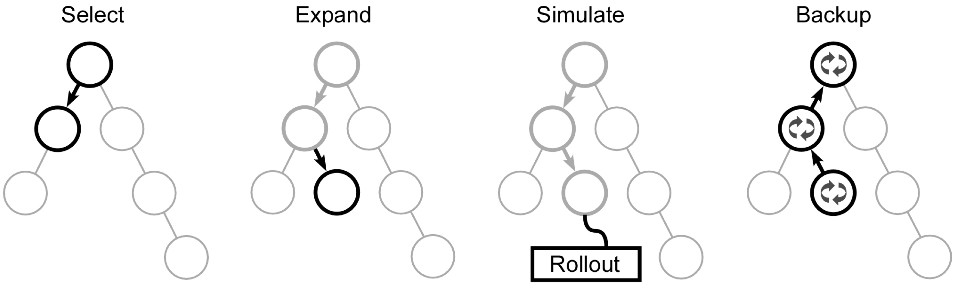
Although traffic network environments are complex, the UCT algorithm can find a solution without requiring specific domain knowledge. The algorithm can build decision trees that efficaciously balance exploration of new states with the exploitation of high performing states. UCT is composed of four primary operations: Select, Expand, Simulate, and Backup. A visual representation of the primary operations is provided in
Figure 8. Note that the
Simulate operation in
Figure 8 is performed on Line 23 of Algorithm 1. The other operations presented in
Figure 8 are performed by their counterparts in the pseudocode functions in Algorithm 1.
The Select function traverses the tree, using a modified UCB1 value as a guiding policy. Each progression step through the tree corresponds to a single action, with each action representing a potential route for the ego vehicle. To introduce variability, the action with the highest UCB1 value is selected for 85% of the decisions, while the remainder are chosen at random. The modified UCB1 formula prioritizes nodes with higher returns at first but gradually favors nodes with high visit count ratios in later iterations. Each node’s UCB1 value is initialized to 106, which is a deliberately high value, to facilitate initial exploration. After a node’s first visit, its UCB1 value diverges from the initial high value, encouraging exploitation in subsequent iterations of the UCT algorithm.
The Expand function increases the size of the decision tree. If the selected leaf node has not been visited, then new children are created underneath it, and a new state is assigned to the newly formed node. This state assigned to the new node is processed through the DRL algorithm, which is explained in the subsequent section. The Backup function updates the nodes traversed in the current round of UCT search. It increases the visit count of the current node , denoted as , and that of its parent node by one each. The total value return accumulates the output of the DRL algorithm over the life of the decision tree.
| Algorithm 1. UCT search algorithm. |
| 1 | |
| 2 | |
| 3 | |
| 4 | |
| 5 | |
| 6 | |
| 7 | |
| 8 | |
| 9 | |
| 10 | |
| 11 | |
| 12 | |
| 13 | |
| 14 | |
| 15 | |
| 16 | |
| 17 | |
| 18 | |
| 19 | |
| 20 | |
| 21 | |
| 22 | |
| 23 | |
| 24 | |
| 25 | |
| 26 | |
| 27 | |
| 28 | |
| 29 | |
| 30 | |
The UCTSearch function is called 8192 times in succession to expand the tree structure for each route recommendation, which is provided to the ego vehicle once per minute of simulation time. Then, a move is selected based on the ratio of the visit count of each child node
to the visit count of its parent node
as shown in Equation (1). The selected child node
c is set as the new root node, and the process is repeated until a move selects a terminal node as the new root node:
A reward is returned after reaching a terminal node, and the value is stored in each node selected as a move in the decision tree. The reward is determined by calculating the fuel efficiency of the ego vehicle for the full simulation and comparing the result to a reference fuel efficiency. If the states recommended by UCT improve on the reference efficiency, then a reward of 1 is returned; otherwise, the reward is set to .
To calculate the simulation’s fuel efficiency, which is the fuel efficiency of the ego vehicle from the root node to the terminal node, the traffic data is retrieved from each node selected as a move in the decision tree. Since the grayscale images are integer-based approximations of the raw data, a history of the raw fuel efficiency data collected at every time step is also saved in each node. This raw data is accumulated and normalized by the total driving time to calculate the overall fuel efficiency for the simulation.
4.2. Deep Reinforcement Learning Algorithm
In this study, a DRL algorithm is utilized to estimate the value of the current traffic state and which route to choose next, as shown in
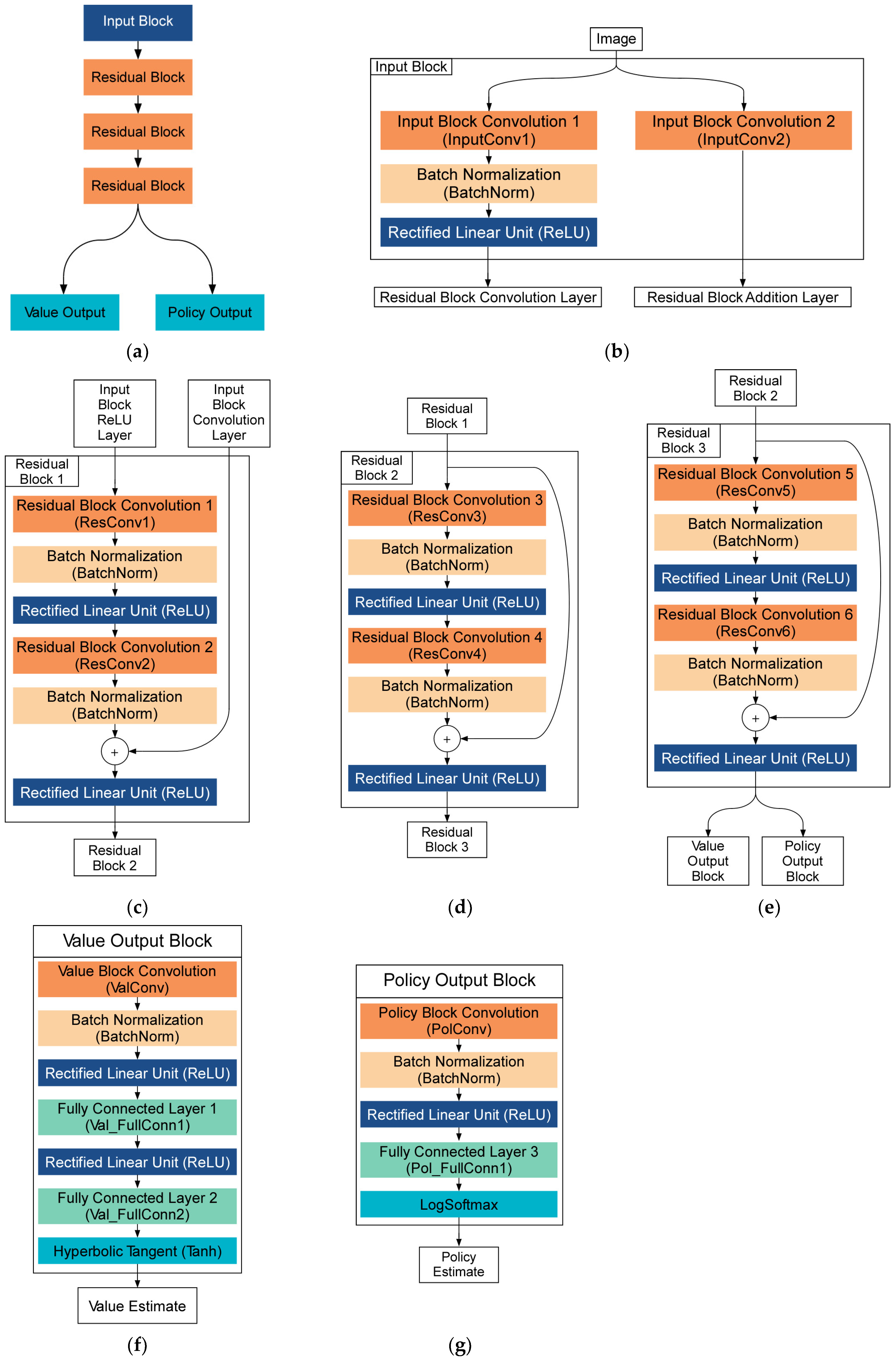
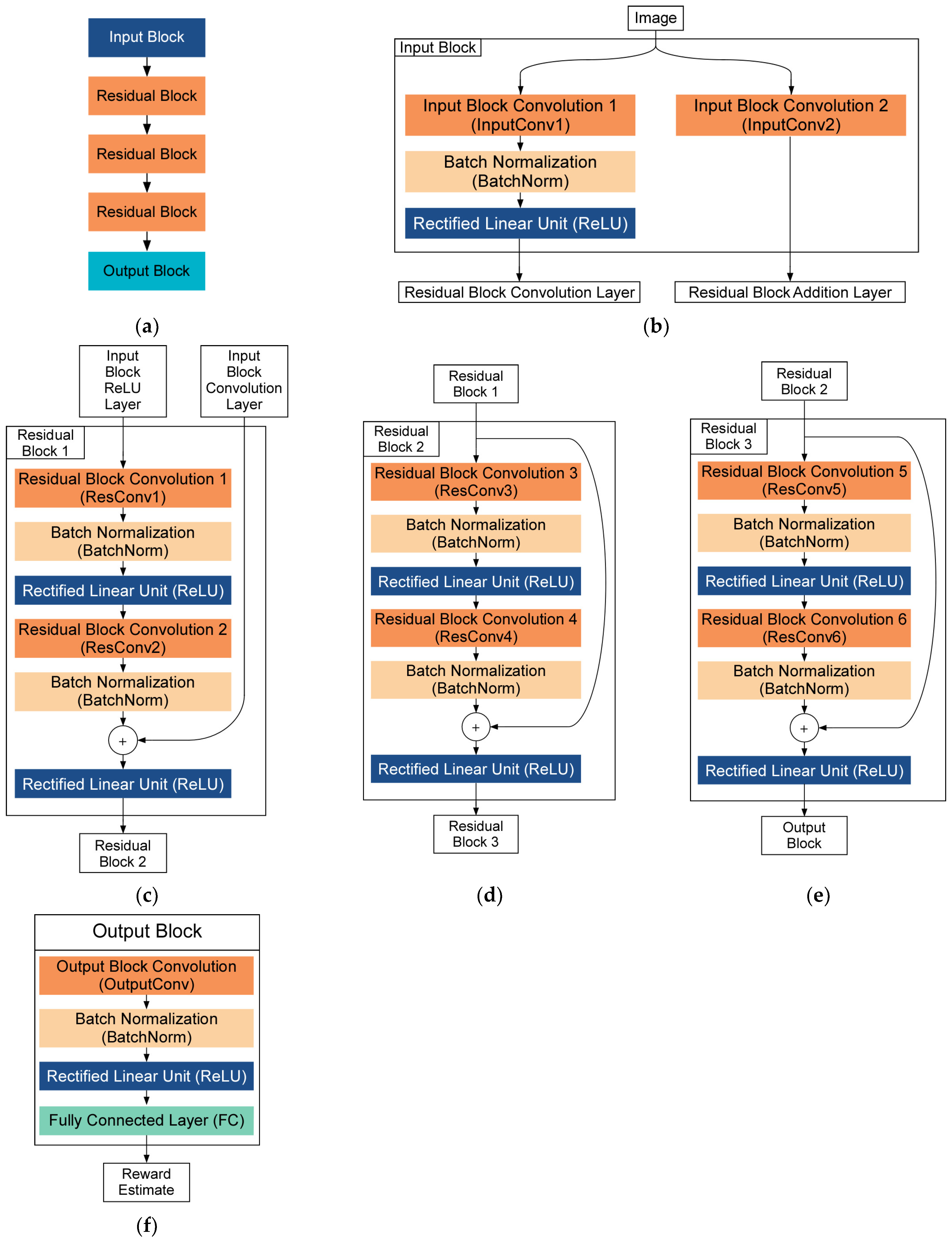
Figure 7. For the DRL algorithm, a deep residual neural network (ResNet) is employed with one input block, three residual blocks, a value output block, and a policy output block, as shown in
Figure 9a. The input block consists of two parallel convolutional layers as shown in
Figure 9b. The output of the first convolutional layer (InputConv1) is normalized and fed to a nonlinear function called the Rectified Linear Unit (ReLU) and becomes the input to the first residual block. The output of the second convolutional layer (InputConv2) is sent to the addition layer of the first residual block. The first residual block consists of two convolutional layers (ResConv1 and ResConv2), two batch normalizations (BatchNorm), and two ReLU functions, as shown in
Figure 9c. The input to the first residual block from the second convolutional layer in the input block is fed directly to the addition layer. This residual signal directly added to the addition layer alleviates information loss during the convolution process. The second and third residual blocks (
Figure 9d,e) feature the same layers as the first residual block but only accept a single input signal from the preceding residual block.
Similar to the ResNet in AlphaGo Zero, the ResNet in this study has two output blocks. The policy block predicts the probability distribution of six possible waypoints to choose from the current position of the ego vehicle. A higher probability output for a given route corresponds to the estimated probability of the route to provide higher efficiency than a user-defined reference efficiency. The value block predicts the expected reward of the simulation based on the current state of the traffic network in the range .
The value output block consists of a single convolution (ValConv), normalization, and nonlinearity stack, followed by a fully connected layer (Val_FullConn1), another nonlinearity, a fully connected layer (Val_FullConn2), and a hyperbolic tangent function (Tanh), as shown in
Figure 9f. The policy output block consists of a single convolution (PolConv), normalization, and nonlinearity stack of layers, followed by one fully connected layer (Pol_FullConn1) and a softmax function, as shown in
Figure 9g. The hyperparameters of each layer in the blocks are listed in
Table 2 for the convolution layers and
Table 3 for the fully connected layers.
Stochastic gradient descent (SGD) is employed to minimize the difference between the predictions of the ResNet and the outputs from the decision tree by updating the ResNet via backpropagation of the results of a loss function. The two types of outputs, the value and policy estimates, require their own loss terms. For the value estimate of the ResNet, the loss term utilizes the mean squared error
between the reward returned by the simulation terminal state
and the value estimate
as shown in Equation (2). The policy estimate loss is determined by a cross-entropy loss equation as shown in Equation (3), where
is the cross-entropy loss,
is the transition probability for each route estimated by the decision tree, and
is the array of probabilities for taking each of the six possible routes estimated by the ResNet:
In this study, the total loss for the ResNet was calculated as the sum of the mean squared error and cross-entropy losses as shown in Equation (4). Optimizing the ResNet learning parameters for both the value and policy estimates allowed for more efficient decision tree searches. This improvement in search efficiency led to higher quality data to train the ResNet. The decision tree generated by UCT iterations and the ResNet synergistically collaborated to discover the most optimal route for the ego vehicle.
The total number of generated images is proportional to the number of states in the decision tree, which is determined by two factors. The first is the number of route choices per node, which is equivalent to the number of branches from each node. Since there were six waypoints in the current traffic network, this number was six in this study. The second factor is the tree depth or number of route selections made before the simulation terminates. The simulation terminated when exceeding the allowed runtime or upon the ego vehicle arriving at the destination. The maximum depth was set to four nodes, including the root node. Considering that each node could have a maximum of six children, a maximum tree size of 259 nodes could be created for each traffic simulation. With one node per state and one state per image, 50 training simulations produced a total of 12,950 images. Overall, 80% of the simulations and their images (10,360) were used for training, and the remaining simulations and images (2590) were reserved for testing.
The DRL algorithm was initiated with random ResNet parameters and an empty decision tree. The number of ResNet learning epochs was set to 256. Also, four moves were selected per learning epoch, and the number of UCT algorithm iterations per move selection was set to 8192. While the number of moves was determined by the maximum tree depth, both the number of learning epochs and the number of UCT iterations per move were selected heuristically by the user. Also, the probability of selecting the best child in the UCT selection function was set to 85%, as shown in Algorithm 1. The DRL algorithm was trained on a Windows 10 Dell G5 computer with an Nvidia RTX 2070 GPU, Intel i9 processor, 64 GB of memory, and 1 TB SSD. The code was written in Python 3.9.13, and Pytorch (version 1.13.1) was used to construct the neural network and handle training.
5. Simulation Results
In the simulation study of the proposed algorithm, a consistent traffic network was used, maintaining the same traffic light control sequence and timing. However, to introduce variability, the traffic conditions in each simulation were altered by incorporating a randomly generated traffic load of 50 vehicles. The initial reference efficiency used in this study was based on the average fuel efficiency observed from 1000 simulations where the ego vehicle followed the shortest route calculated by SUMO. This figure turned out to be 379 mL of fuel. Though the average fuel efficiency over many trips is a strong candidate as a reference, the algorithm can be trained with any reference value selected by the user. Through various simulations, it was determined that the best fuel efficiency results could be obtained when the reference was set to 346 mL.
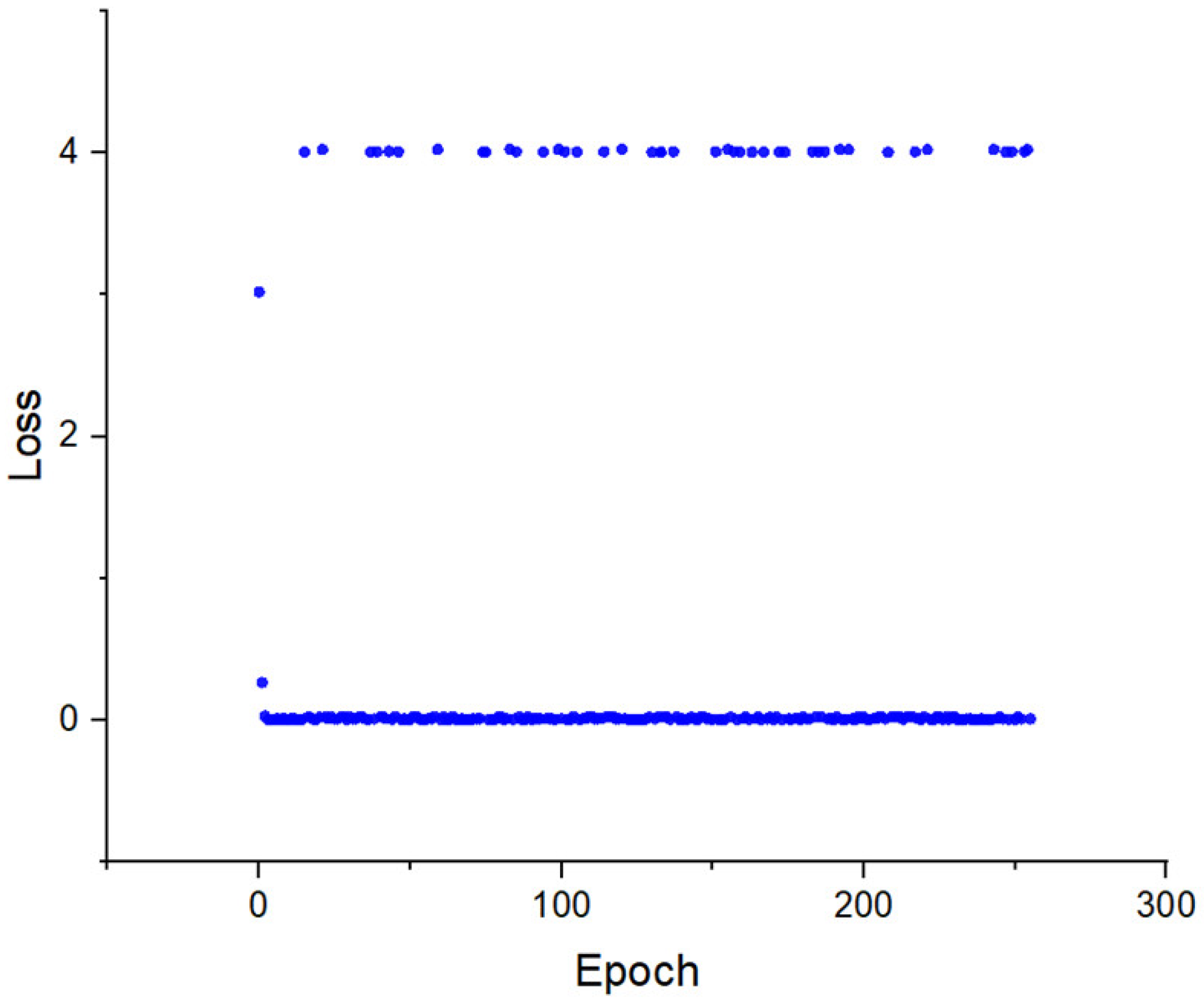
Over four days and nine hours of training, it was observed that the loss curve rapidly approached zero, as shown in
Figure 10. The trained algorithm consistently chose routes with an average fuel consumption of 349.96 mL per trip. This represents a 7.66% improvement in energy efficiency over the baseline fuel consumption of 379 mL over 1000 simulated trips determined by SUMO.
It is important to note that in some simulations, the fuel consumption for the optimal route exceeded the 346 mL reference set for training. According to the definition of the UCT reward function , the reward was when the selected route consumed more fuel than the reference value. The ResNet predicted a value close to one in these cases since the true fuel consumption was still close to the training reference. This resulted in an value of about 4.00 for these scenarios based on Equation (2). The remainder of the error was just above zero, meaning the policy was generally correct, and an optimal route was selected. A small difference in total fuel consumption resulted in high losses for a few scenarios, but the trained ResNet showed a significant improvement in optimal route selection over the shortest path for all scenarios tested.
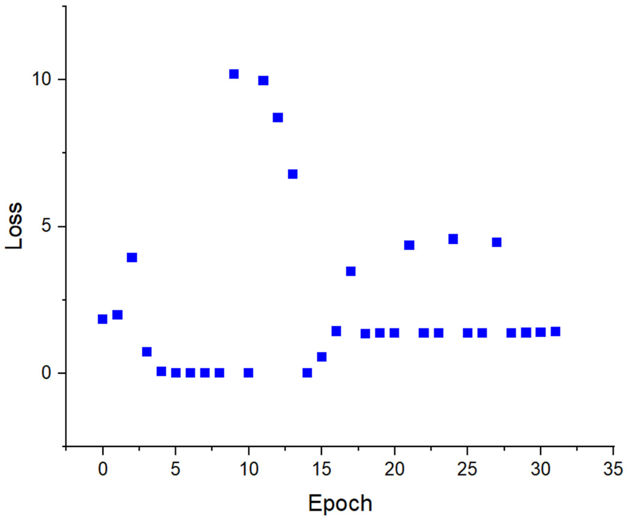
To show the effects of a different reference, the result of a short training session with the 379 mL reference is shown in
Figure 11. The loss also approached zero within a couple of epochs but later destabilized. This behavior may be fixed with some combination of a larger training set, a larger decision tree, and a larger ResNet. As shown in
Figure 10, however, restricting the reference to achieve a positive reward was effective without increasing the required computing power.
The training and test accuracies were calculated by the outcome of the simulation, namely whether the route taken by the ego vehicle saved energy compared with taking the shortest route. While not every selected route between the origin and destination might be the most efficient one, the overall result indicated improved efficiency. In the training phase, the algorithm improved the ego vehicle’s fuel efficiency in all 40 training simulations utilizing 10,360 images. The algorithm also improved the ego vehicle’s fuel efficiency for all 10 remaining testing simulations with 2590 images.
The DRL agent paired with the UCT algorithm selected routes that used 7.66% less fuel on average than the shortest route recommended by SUMO. This amount of saving includes scenarios from both training and test data. The learned parameters were therefore robust to previously unseen traffic states since the ResNet parameters remained unchanged when exposed to the test data, indicating its adaptability and effectiveness in varied scenarios. In addition to fuel consumption, it was observed that nearly all optimized routes remained within a comparable time window and network region as the shortest-path baseline, as enforced by the simulation constraints. A quantitative analysis of route length and travel time will be conducted in future work to provide a more comprehensive evaluation of the trade-offs between fuel efficiency, travel time, and distance.
6. Performance Comparison
To further evaluate the performance of the proposed model-based deep reinforcement learning algorithm, the robustness of the model-based agent was compared with that of an agent trained using a conventional model-free algorithm.
6.1. Model-Free Deep Reinforcement Learning Algorithm
The model-free Deep Q-Network (DQN) algorithm was selected as a baseline for the results obtained from the proposed model-based method. The DQN is well known for its simplicity, stability, and common use as a benchmark algorithm. The DQN is also frequently applied to similar traffic optimization problems. The input provided to the model-free DQN agent was the same as that for the model-based approach. The traffic state was formatted into an image, which was processed by the agent to select a route for the ego vehicle. The traffic light and random traffic parameters were also held constant in the training data to minimize the difference between the results of the two methods.
The model-free agent also has a neural network architecture similar to that of the model-based agent. A ResNet is employed as the neural network for the DQN algorithm. The DQN ResNet consists of one input block, three residual blocks, and an output block, as shown in
Figure 12a. The input block contains two parallel convolutional layers, InputConv1 and InputConv2, as shown in
Figure 12b. The output of InputConv1 is normalized and then transformed by an ReLU function. This ReLU output serves as the input to the first residual block. The output of InputConv2 is directly connected to the addition layer of the first residual block. The first residual block consists of convolutional layers ResConv1 and ResConv2, two BatchNorm functions, and two ReLU functions, as shown in
Figure 12c. The remaining two residual blocks (
Figure 12d,e) accept only a single input signal from the preceding residual block but otherwise share the identical structure with the first residual block.
Unlike the model-based algorithm, the DQN ResNet has only one output block. The output block consists of a single convolution (OutputConv), normalization, and nonlinearity layers, followed by one fully connected layer (FC), as shown in
Figure 12f. The hyperparameters of each layer in the blocks are listed in
Table 4.
The DQN ResNet output block predicts the estimated reward for the current state. Based on the standard DQN algorithm, the difference between the calculated reward and neural network estimated reward are minimized with a mean squared error loss function. The calculated reward function in this case consists of user-defined tuning parameters, simulation data, and a noise parameter. Two user-defined tuning parameters
α and
β are set to −1 × 10
−3 and −1 × 10
−4, respectively. Simulation data is represented in the reward function by the fuel consumed by the ego vehicle since the last route selection in milliliters (
ft) and the total fuel consumed since the start of the simulation in milliliters (
fs). To encourage exploration of the state space, a Gaussian noise parameter
η ∼ N(0, 10
−4) is also included in the reward function. The reward function is shown in Equation (5):
The training and testing of the model-free agent were conducted using 50 traffic scenarios. Forty scenarios were used for training, and the remaining 10 were reserved for testing the trained agent. Each training and testing scenario was defined by a fixed traffic-light program and randomly generated traffic flows, which is consistent with the training and testing methodology for the model-based agent.
The trained model-free agent could find routes that significantly improved the energy efficiency of the ego vehicle compared with selecting the shortest route. The trained agent achieved an average of 7.97% improvement in energy efficiency over the shortest route in the testing dataset. This represents a slight improvement compared with the model-based agent, which achieved a 7.66% improvement. In addition, while the model-based method is computationally expensive to train, performing only 256 parameter updates over a four-day period, the model-free agent completed 10,000 parameter updates in less than an hour. Additional updates beyond these numbers did not yield significant improvements in either agent.
6.2. Robustness Test
The similarity in performance between the two agents suggests the importance of evaluating them under diverse simulation conditions. Both algorithms identified efficient routes in the testing cases. However, each agent encountered certain states multiple times during training because the number of parameter updates far exceeded the number of training scenarios. Specifically, the model-based method updated its parameters 256 times, while the model-free method performed 10,000 updates. This discrepancy arose from the higher computational cost of the UCT algorithm used in the model-based approach. Additionally, traffic signal programs remained identical across all scenarios, including those reserved for testing. Consequently, strong performance in scenarios featuring different traffic signal programs cannot be guaranteed. Traffic optimization agents rarely experience repeated traffic states in real-world settings, and a variety of traffic signal programs are typically employed in both simulations and practical applications. Therefore, agents developed in this work must demonstrate robustness under previously unseen traffic conditions.
The robustness test consisted of 30 traffic simulations. Each simulation combined a unique random seed defining the congestion levels for each road segment with one of three distinct traffic signal programs. Ten random seeds generated the traffic flows across all simulations. Fifty vehicles with randomly assigned origins, destinations, and departure times represented varying traffic congestion. Each traffic signal program maintained a fixed 90-second cycle but differed in phase length, as detailed in
Table 5. The chosen program was applied to 34 intersections within the network, where more than two roads intersected. The remaining two-way intersections, located at the upper-right and lower-left corners, maintained continuous green signals. The three traffic signal programs included two scenarios where one phase dominated the cycle (P1 and P3) and one balanced configuration (P2). These scenarios introduced variability into the traffic environment while maintaining consistent cycle lengths across all simulations.
The model-free and model-based agents calculated the optimal energy-efficient routes for all 30 simulations. The ego vehicle followed these routes in each simulation, and the total fuel consumption was recorded, as shown in
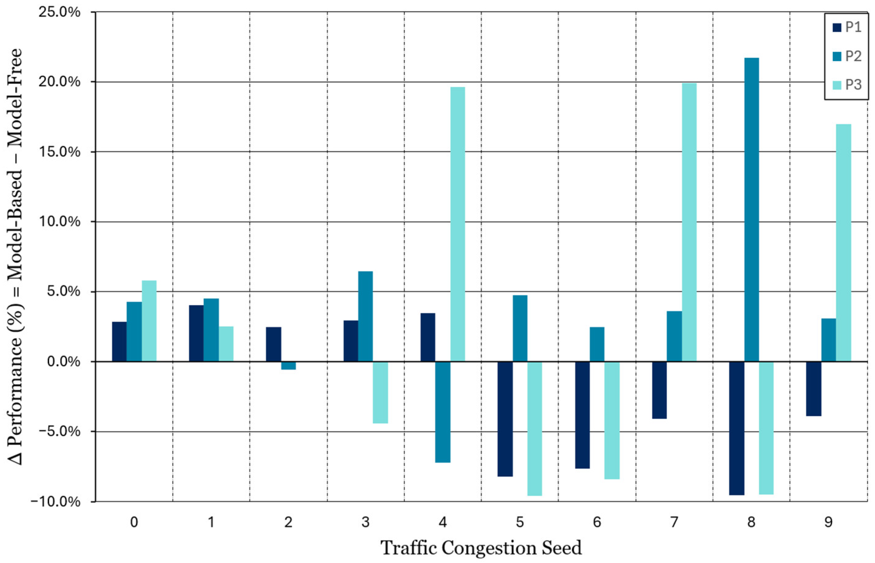
Table 6. The performance differences between the two methods are summarized in
Figure 13, where a positive performance difference indicates superior performance by the model-based algorithm. A review of the total fuel consumption reveals that the routes determined by the model-based agent achieved 1.95% higher energy efficiency on average than the model-free agent across all 30 simulations. Considering that both algorithms improved the energy efficiency by less than 8% over the shortest route in the training dataset, the 1.95% average margin observed in the robustness test is regarded as a significant improvement in agent performance. The savings figure of 1.95%, relative to an average improvement of 7.66%, represents a 25.5% relative improvement on average. These results confirm that the model-based method outperformed the model-free methods in medium-scale problems. Given that model-free approaches often struggle with complex traffic scenarios in large-scale networks, the model-based method was expected to be even more effective, similar to its success in solving large-scale challenges in Go.
The model-free DQN-trained agent could find routes with higher efficiency than the model-based agent in 14 out of the 30 simulations. However, the model-based agent discovered substantially better routes in several scenarios, achieving energy efficiency improvements exceeding 15% in four cases. Given that the robustness test introduced entirely new traffic conditions not present in the training data, the results indicate that the model-based agent retained a consistent performance advantage and demonstrated superior generalization capabilities.
Real-world traffic networks are typically larger and more complex than the grid scenario presented in this work. The model-based method is recognized for its superhuman performance in complex decision-making problems, such as Go, whereas the DQN method often struggles when facing large state and action spaces. Since generalization and optimal solution discovery in large state spaces are critical for traffic optimization problems, the proposed model-based approach is considered more advantageous for scaled-up, real-world traffic environments.
7. Conclusions and Future Works
This study demonstrated the effectiveness of a model-based deep reinforcement learning (MB-DRL) algorithm for optimizing the route of a connected and automated vehicle in a traffic network to improve energy efficiency. By combining a decision tree and a deep reinforcement learning algorithm with a traffic simulation model, the proposed approach successfully trained an agent to minimize energy consumption while navigating the traffic network. The optimized routes generated by the MB-DRL agent achieved an average reduction of 7.66% in vehicle energy consumption. Additionally, the agent’s learned behavior was robust to variations in traffic load without requiring further training, demonstrating superior performance compared with conventional methods. Based on the proven capability of the model-based algorithm in other complex tasks, it is anticipated that its performance advantage will further increase in larger-scale traffic environments.
These improvements align with reported gains in other energy-optimization strategies for connected and automated vehicles (CAVs), such as eco-driving and powertrain-aware routing [
15,
32]. Unlike methods that rely on static energy cost maps or brute-force optimization, the proposed approach enables dynamic route adaptation in response to changing traffic conditions while retaining its generalization capability for unseen scenarios. This flexibility is particularly valuable in urban networks where real-time traffic variability significantly impacts vehicle energy consumption. By integrating learning-based decision making with traffic-aware simulation, these results demonstrate the potential for intelligent routing systems to play a key role in future sustainable transportation infrastructure. A practical deployment of the proposed approach would require a centralized server equipped with a trained model to collect real-time data from vehicles and traffic signals, compute optimal routes, and transmit routing decisions to individual vehicles. Although substantial infrastructure would be needed, such a system is expected to enable coordinated, city-scale traffic optimization.
In future work, additional control strategies will be explored to further improve energy efficiency at the system level. First, the optimal control of traffic signal phases will be investigated using MB-DRL to achieve network-wide reductions in fuel consumption. This follow-up research will involve significantly larger, city-scale traffic networks, where the complexity of both the traffic network topology and traffic flow models will be increased. The learning agent will also need to be updated to effectively handle these expanded challenges. Next, an integrated approach that combines the route optimization developed in this study with traffic signal control will be examined. While this work focused on optimizing the route of a single vehicle, future studies must address the more complex problem of multi-vehicle route optimization. For instance, optimal routes for multiple vehicles may overlap on the same road segment, potentially causing congestion in unexpected locations. To avoid this, future agents should be designed with awareness of all desired routes and interactions among vehicles. Finally, optimization of vehicle powertrains using DRL will also be considered. In parallel, multiagent approaches, particularly those focused on controlling individual vehicles or localized traffic signals, will be explored. These decentralized agents, operating with smaller sets of localized traffic information, are expected to offer additional energy savings. A comprehensive strategy that simultaneously manages traffic signals, route selection, and vehicle powertrains using MB-DRL, potentially in a multi-agent framework, is expected to enable effective, network-wide energy optimization under dynamic traffic conditions.
Author Contributions
Conceptualization, D.R.L.; methodology, D.R.L.; software, D.R.L.; validation, D.R.L. and H.-S.Y.; formal analysis, D.R.L.; investigation, D.R.L.; resources, H.-S.Y.; data curation, D.R.L.; writing—original draft preparation, D.R.L.; writing—review and editing, H.-S.Y.; visualization, D.R.L.; supervision, H.-S.Y.; project administration, H.-S.Y. All authors have read and agreed to the published version of the manuscript.
Funding
This research received no external funding.
Institutional Review Board Statement
Not applicable.
Informed Consent Statement
Not applicable.
Data Availability Statement
The data presented in this study are available on request from the corresponding author.
Conflicts of Interest
The authors declare no conflicts of interest.
References
- EPA. Inventory of U.S. Greenhouse Gas Emissions and Sinks: 1990–2022 U.S. Environmental Protection Agency, EPA 430R-24004. 2024. Available online: https://www.epa.gov/ghgemissions/inventory-us-greenhouse-gas-emissions-and-sinks-1990-2022 (accessed on 10 June 2025).
- Ahn, K.; Rakha, H. The effects of route choice decisions on vehicle energy consumption and emissions. Transp. Res. Part D Transp. Environ. 2008, 13, 151–167. [Google Scholar] [CrossRef]
- Ericsson, E. Independent driving pattern factors and their influence on fuel-use and exhaust emission factors. Transp. Res. Part D Transp. Environ. 2001, 6, 325–345. [Google Scholar] [CrossRef]
- Lopez, P.A.; Behrisch, M.; Bieker-Walz, L.; Erdmann, J.; Flötteröd, Y.P.; Hilbrich, R.; Lücken, L.; Rummel, J.; Wagner, P.; Wießner, E. Microscopic Traffic Simulation using SUMO. In Proceedings of the 2018 21st International Conference on Intelligent Transportation Systems (ITSC), Maui, HI, USA, 4–7 November 2018. [Google Scholar]
- Marinković, D.; Dezső, G.; Milojević, S. Application of machine learning during maintenance and exploitation of electric vehicles. Adv. Eng. Lett. 2024. [Google Scholar] [CrossRef]
- Silver, D.; Schrittwieser, J.; Simonyan, K.; Antonoglou, I.; Huang, A.; Guez, A.; Hubert, T.; Baker, L.; Lai, M.; Bolton, A.; et al. Mastering the game of go without human knowledge. Nature 2017, 550, 354–359. [Google Scholar] [CrossRef]
- Anda, J.; LeBrun, J.; Ghosal, D.; Chuah, C.N.; Zhang, M. VGrid: Vehicular adhoc networking and computing grid for intelligent traffic control. In Proceedings of the 2005 IEEE 61st Vehicular Technology Conference, Stockholm, Sweden, 30 May–1 June 2005. [Google Scholar]
- Talebpour, A.; Mahmassani, H.S. Influence of connected and autonomous vehicles on traffic flow stability and throughput. Transp. Res. Part C Emerg. Technol. 2016, 71, 143–163. [Google Scholar] [CrossRef]
- Aguiar, A.; Fernandes, P.; Guerreiro, A.P.; Tomas, R.; Agnelo, J.; Santos, J.L.; Araujo, F.; Coelho, M.C.; Fonseca, C.M.; d’Orey, P.M.; et al. MobiWise: Eco-routing decision support leveraging the Internet of Things. Sustain. Cities Soc. 2022, 87, 104180. [Google Scholar] [CrossRef]
- Caspari, A.; Fahr, S.; Mitsos, A. Optimal Eco-Routing for Hybrid Vehicles with Powertrain Model Embedded. IEEE Trans. Intell. Transp. Syst. 2022, 23, 14632–14648. [Google Scholar] [CrossRef]
- Chen, J.; Hu, M.; Shi, C. Development of eco-routing guidance for connected electric vehicles in urban traffic systems. Phys. A Stat. Mech. Its Appl. 2023, 618, 128718. [Google Scholar] [CrossRef]
- Chen, X.; Xue, J.; Lei, Z.; Qian, X.; Ukkusuri, S.V. Online eco-routing for electric vehicles using combinatorial multi-armed bandit with estimated covariance. Transp. Res. Part D Transp. Environ. 2022, 111, 103447. [Google Scholar] [CrossRef]
- Dehkordi, S.G.; Larue, G.S.; Cholette, M.E.; Rakotonirainy, A.; Glaser, S. Including network level safety measures in eco-routing. J. Intell. Transp. Syst. 2024, 28, 283–296. [Google Scholar] [CrossRef]
- Kosmanos, D.; Maglaras, L.A.; Mavrovouniotis, M.; Moschoyiannis, S.; Argyriou, A.; Maglaras, A.; Janicke, H. Route Optimization of Electric Vehicles Based on Dynamic Wireless Charging. IEEE Access 2018, 6, 42551–42564. [Google Scholar] [CrossRef]
- Boriboonsomsin, K.; Barth, M.J.; Zhu, W.; Vu, A. Eco-Routing Navigation System Based on Multisource Historical and Real-Time Traffic Information. IEEE Trans. Intell. Transp. Syst. 2012, 13, 1694–1704. [Google Scholar] [CrossRef]
- Guo, Q.; Li, L.; Ban, X.J. Urban traffic signal control with connected and automated vehicles: A survey. Transp. Res. Part C Emerg. Technol. 2019, 101, 313–334. [Google Scholar] [CrossRef]
- Yazdi, M.A.A. A Web-Based Personal Driving Assistant Using Real-Time Data and a Dynamic Programming Model; ProQuest LLC.: Auburn, AL, USA, 2018. [Google Scholar]
- Pulvirenti, L.; Tresca, L.; Rolando, L.; Millo, F. Eco-Driving Optimization Based on Variable Grid Dynamic Programming and Vehicle Connectivity in a Real-World Scenario. Energies 2023, 16, 4121. [Google Scholar] [CrossRef]
- Peng, N.; Xi, Y.; Rao, J.; Ma, X.; Ren, F. Urban Multiple Route Planning Model Using Dynamic Programming in Reinforcement Learning. IEEE Trans. Intell. Transp. Syst. 2022, 23, 8037–8047. [Google Scholar] [CrossRef]
- Abdul-Hak, M.; Bazzi, Y.; Cordes, O.; Alholou, N. Dynamic eco-routing methodology using petri net. In Proceedings of the SAE 2013 World Congress and Exhibition, Detroit, MI, USA, 16–18 April 2013; SAE International: London, UK, 2013. [Google Scholar]
- Arulkumaran, K.; Deisenroth, M.P.; Brundage, M.; Bharath, A.A. Deep reinforcement learning: A brief survey. IEEE Signal Process. Mag. 2017, 34, 26–38. [Google Scholar] [CrossRef]
- Mnih, V.; Kavukcuoglu, K.; Silver, D.; Graves, A.; Antonoglou, I.; Wierstra, D.; Riedmiller, M. Playing atari with deep reinforcement learning. arXiv 2013, arXiv:1312.5602. [Google Scholar]
- Ruan, X.; Ren, D.; Zhu, X.; Huang, J. Mobile robot navigation based on deep reinforcement learning. In Proceedings of the 2019 Chinese Control and Decision Conference (CCDC), IEEE, Nanchang, China, 3–5 June 2019. [Google Scholar]
- Silver, D.; Hubert, T.; Schrittwieser, J.; Antonoglou, I.; Lai, M.; Guez, A.; Lanctot, M.; Sifre, L.; Kumaran, D.; Graepel, T.; et al. A general reinforcement learning algorithm that masters chess, shogi, and Go through self-play. Science 2018, 362, 1140–1144. [Google Scholar] [CrossRef]
- Boukerche, A.; Zhong, D.; Sun, P. FECO: An Efficient Deep Reinforcement Learning-Based Fuel-Economic Traffic Signal Control Scheme. IEEE Trans. Sustain. Comput. 2022, 7, 144–156. [Google Scholar] [CrossRef]
- Yeom, K. Model predictive control and deep reinforcement learning based energy efficient eco-driving for battery electric vehicles. Energy Rep. 2022, 8, 34–42. [Google Scholar] [CrossRef]
- Zheng, X.; Huang, W.; Wang, S.; Zhang, J.; Zhang, H. Research on Energy-Saving Routing Technology Based on Deep Reinforcement Learning. Electronics 2022, 11, 2035. [Google Scholar] [CrossRef]
- Kim, M.; Schrader, M.; Yoon, H.S.; Bittle, J.A. Optimal traffic signal control using priority metric based on real-time measured traffic information. Sustainability 2023, 15, 7637. [Google Scholar] [CrossRef]
- Schrader, M.; Bittle, J. A Global Sensitivity Analysis of Traffic Microsimulation Input Parameters on Performance Metrics. IEEE Trans. Intell. Transp. Syst. 2024. [Google Scholar] [CrossRef]
- Lee, E.H.; Lee, E. Congestion boundary approach for phase transitions in traffic flow. Transp. B Transp. Dyn. 2024, 12, 2379377. [Google Scholar] [CrossRef]
- Huang, L.; Zhang, S.N.; Li, S.B.; Cui, F.Y.; Zhang, J.; Wang, T. Phase transition of traffic congestion in lattice hydrodynamic model: Modeling, calibration and validation. Mod. Phys. Lett. B 2024, 38, 2450012. [Google Scholar] [CrossRef]
- Gonder, J.; Earleywine, M.; Sparks, W. Analyzing vehicle fuel saving opportunities through intelligent driver feedback. SAE Int. J. Passeng. Cars-Electron. Electr. Syst. 2012, 5, 450–461. [Google Scholar] [CrossRef]
Figure 1.
Studied road network in SUMO. (a) Network overview with start and end positions of controlled vehicle. (b) Detailed view of four-way intersection. (c) Detailed view of three-way intersection. (d) Detailed view of two-way intersection.
Figure 1.
Studied road network in SUMO. (a) Network overview with start and end positions of controlled vehicle. (b) Detailed view of four-way intersection. (c) Detailed view of three-way intersection. (d) Detailed view of two-way intersection.
Figure 2.
Lookup table for vehicle fuel consumption rate as a function of acceleration and velocity.
Figure 2.
Lookup table for vehicle fuel consumption rate as a function of acceleration and velocity.
Figure 3.
User-defined waypoints in the SUMO road network.
Figure 3.
User-defined waypoints in the SUMO road network.
Figure 4.
Three-dimensional image representing a traffic state.
Figure 4.
Three-dimensional image representing a traffic state.
Figure 5.
Two-dimensional image representing a traffic state: (Det. A) congestion for one road, (Det. B) traffic signal condition, (Det. C) ego vehicle position, and (Det. D) the current route and fuel consumption.
Figure 5.
Two-dimensional image representing a traffic state: (Det. A) congestion for one road, (Det. B) traffic signal condition, (Det. C) ego vehicle position, and (Det. D) the current route and fuel consumption.
Figure 6.
Graphical components in traffic state representation: (a) example road conditions, (b) traffic light conditions, (c) controlled ego vehicle, and (d) energy efficiency and route conditions.
Figure 6.
Graphical components in traffic state representation: (a) example road conditions, (b) traffic light conditions, (c) controlled ego vehicle, and (d) energy efficiency and route conditions.
Figure 7.
Overview of data flow between the decision tree, SUMO, image generator, and neural network in the model-based deep reinforcement learning algorithm.
Figure 7.
Overview of data flow between the decision tree, SUMO, image generator, and neural network in the model-based deep reinforcement learning algorithm.
Figure 8.
Four primary operations of the UCT algorithm.
Figure 8.
Four primary operations of the UCT algorithm.
Figure 9.
Architecture of ResNet used in this study: (a) overall ResNet architecture, (b) input block structure, (c) first residual block structure, (d) second residual block structure, (e) third residual block structure, (f) value output block structure, and (g) policy output block structure.
Figure 9.
Architecture of ResNet used in this study: (a) overall ResNet architecture, (b) input block structure, (c) first residual block structure, (d) second residual block structure, (e) third residual block structure, (f) value output block structure, and (g) policy output block structure.
Figure 10.
Training loss vs. epoch with the 346 mL reference.
Figure 10.
Training loss vs. epoch with the 346 mL reference.
Figure 11.
Training loss vs. epoch with the 379 mL reference.
Figure 11.
Training loss vs. epoch with the 379 mL reference.
Figure 12.
Architecture of the DQN ResNet: (a) overall ResNet architecture, (b) input block structure, (c) first residual block structure, (d) second residual block structure, (e) third residual block structure, and (f) output block structure.
Figure 12.
Architecture of the DQN ResNet: (a) overall ResNet architecture, (b) input block structure, (c) first residual block structure, (d) second residual block structure, (e) third residual block structure, and (f) output block structure.
Figure 13.
Percent difference in total fuel consumption between the model-based and model-free algorithms for each simulation in the robustness test.
Figure 13.
Percent difference in total fuel consumption between the model-based and model-free algorithms for each simulation in the robustness test.
Table 1.
Traffic light control programs for each set of intersections in the traffic network.
Table 1.
Traffic light control programs for each set of intersections in the traffic network.
| Program | Phase 1 Duration [s]
NS = Green
EW = Red | Phase 2 Duration [s]
NS = Yellow
EW = Red | Phase 3 Duration [s]
NS = Red
EW = Green | Phase 4 Duration [s]
NS = Red
EW = Yellow |
|---|
| Program 1 | 40 | 5 | 10 | 5 |
| Program 2 | 25 | 5 | 25 | 5 |
| Program 3 | 10 | 5 | 40 | 5 |
Table 2.
Hyperparameters of convolutional layers in ResNet.
Table 2.
Hyperparameters of convolutional layers in ResNet.
| Conv Layer ID | Input Channels | Output Channels | Kernel Size | Stride | Padding |
|---|
| InputConv1 | 10 | 16 | 1 × 1 | 1 | 0 |
| InputConv2 | 10 | 16 | 3 × 3 | 1 | 1 |
| ResConv1 | 16 | 16 | 3 × 3 | 1 | 1 |
| ResConv2 | 16 | 16 | 3 × 3 | 1 | 1 |
| ResConv3 | 16 | 16 | 3 × 3 | 1 | 1 |
| ResConv4 | 16 | 16 | 3 × 3 | 1 | 1 |
| ResConv5 | 16 | 16 | 3 × 3 | 1 | 1 |
| ResConv6 | 16 | 16 | 3 × 3 | 1 | 1 |
| ValConv | 16 | 64 | 1 × 1 | 1 | 0 |
| PolConv | 16 | 64 | 1 × 1 | 1 | 0 |
Table 3.
Hyperparameters of fully connected layers in ResNet.
Table 3.
Hyperparameters of fully connected layers in ResNet.
| Fully Connected Layer ID | Input Channels | Neuron Count |
|---|
| Val_FullConn1 | 65,536 | 4096 |
| Val_FullConn2 | 4096 | 1 |
| Pol_FullConn1 | 65,536 | 6 |
Table 4.
Hyperparameters of convolutional layers in ResNet trained with DQN.
Table 4.
Hyperparameters of convolutional layers in ResNet trained with DQN.
| Conv Layer ID | Input Channels | Output Channels | Kernel Size | Stride | Padding |
|---|
| InputConv1 | 10 | 16 | 1 × 1 | 1 | 0 |
| InputConv2 | 10 | 16 | 3 × 3 | 1 | 1 |
| ResConv1 | 16 | 16 | 3 × 3 | 1 | 1 |
| ResConv2 | 16 | 16 | 3 × 3 | 1 | 1 |
| ResConv3 | 16 | 16 | 3 × 3 | 1 | 1 |
| ResConv4 | 16 | 16 | 3 × 3 | 1 | 1 |
| ResConv5 | 16 | 16 | 3 × 3 | 1 | 1 |
| ResConv6 | 16 | 16 | 3 × 3 | 1 | 1 |
| OutputConv | 16 | 64 | 1 × 1 | 1 | 0 |
Table 5.
Details of three varied traffic signal programs.
Table 5.
Details of three varied traffic signal programs.
| Program | Phase 1 (s) | Phase 2 (s) | Phase 3 (s) | Phase 4 (s) | Total Cycle (s) |
|---|
| P1 | 72 | 3 | 12 | 3 | 90 |
| P2 | 42 | 3 | 42 | 3 | 90 |
| P3 | 12 | 3 | 72 | 3 | 90 |
Table 6.
Fuel consumed along the routes determined by model-based and model-free agents.
Table 6.
Fuel consumed along the routes determined by model-based and model-free agents.
| Random Traffic Seed | Traffic Signal Program | Fuel Consumption with Model-Free Route [mL] | Fuel Consumption with Model-Based Route [mL] | Difference (%) |
|---|
| 0 | P1 | 340.18 | 330.58 | 2.82% |
| 0 | P2 | 343.02 | 328.43 | 4.25% |
| 0 | P3 | 340.82 | 321.14 | 5.77% |
| 1 | P1 | 341.76 | 328.01 | 4.02% |
| 1 | P2 | 342.34 | 326.86 | 4.52% |
| 1 | P3 | 340.44 | 331.95 | 2.49% |
| 2 | P1 | 338.90 | 330.49 | 2.48% |
| 2 | P2 | 322.50 | 324.31 | −0.56% |
| 2 | P3 | 326.28 | 326.33 | −0.01% |
| 3 | P1 | 334.96 | 325.06 | 2.95% |
| 3 | P2 | 343.28 | 321.14 | 6.45% |
| 3 | P3 | 320.22 | 334.33 | −4.40% |
| 4 | P1 | 340.50 | 328.76 | 3.45% |
| 4 | P2 | 310.39 | 332.70 | −7.19% |
| 4 | P3 | 414.34 | 333.00 | 19.63% |
| 5 | P1 | 297.78 | 322.20 | −8.20% |
| 5 | P2 | 342.61 | 326.33 | 4.75% |
| 5 | P3 | 299.65 | 328.29 | −9.56% |
| 6 | P1 | 305.48 | 328.79 | −7.63% |
| 6 | P2 | 337.10 | 328.79 | 2.46% |
| 6 | P3 | 299.91 | 325.06 | −8.38% |
| 7 | P1 | 317.68 | 330.59 | −4.07% |
| 7 | P2 | 350.96 | 338.28 | 3.62% |
| 7 | P3 | 401.07 | 321.14 | 19.93% |
| 8 | P1 | 306.29 | 335.55 | −9.55% |
| 8 | P2 | 425.39 | 333.00 | 21.72% |
| 8 | P3 | 299.56 | 328.01 | −9.50% |
| 9 | P1 | 309.09 | 321.14 | −3.90% |
| 9 | P2 | 343.21 | 332.67 | 3.07% |
| 9 | P3 | 400.87 | 332.86 | 16.96% |
| Disclaimer/Publisher’s Note: The statements, opinions and data contained in all publications are solely those of the individual author(s) and contributor(s) and not of MDPI and/or the editor(s). MDPI and/or the editor(s) disclaim responsibility for any injury to people or property resulting from any ideas, methods, instructions or products referred to in the content. |
© 2025 by the authors. Licensee MDPI, Basel, Switzerland. This article is an open access article distributed under the terms and conditions of the Creative Commons Attribution (CC BY) license (https://creativecommons.org/licenses/by/4.0/).


