Abstract
Global climate change has altered precipitation patterns, leading to an increased frequency and intensity of extreme rainfall events and introducing greater uncertainty to flood risk in river basins. Traditional assessments often rely on static indicators and single-design scenarios, failing to reflect the dynamic evolution of floods under varying intensities. Additionally, oversimplified topographic representations compromise the accuracy of high-risk-zone identification, limiting the effectiveness of precision flood management. To address these limitations, this study constructs multi-return-period flood scenarios and applies a coupled 1D/2D hydrodynamic model to analyze the spatial evolution of flood hazards and extract refined hazard indicators. A multi-source weighting framework is proposed by integrating the triangular fuzzy analytic hierarchy process (TFAHP) and the entropy weight method–criteria importance through intercriteria correlation (EWM-CRITIC), with game-theoretic strategies employed to achieve optimal balance among different weighting sources. These are combined with the technique for order preference by similarity to an ideal solution (TOPSIS) to develop a continuous flood risk assessment model. The approach is applied to the Georges River Basin in Australia. The findings support data-driven flood risk management strategies that benefit policymakers, urban planners, and emergency services, while also empowering local communities to better prepare for and respond to flood risks. By promoting resilient, inclusive, and sustainable urban development, this research directly contributes to the achievement of United Nations Sustainable Development Goal 11 (Sustainable Cities and Communities).
1. Introduction
Global climate change has induced variations in tropical cyclones and hydrological cycles, leading to an increased frequency and intensity of extreme rainfall events worldwide [1]. Coupled with accelerating urbanization, urban flood disasters have emerged as a global concern [2,3,4]. Basin floodplains and coastal cities, in particular, have become highly susceptible to flooding, posing significant threats to human life, safety, property, and urban stability [5,6]. In July 2023, China’s Haihe River basin faced the most severe rainfall since 1963, triggering widespread catastrophic flooding that affected 8.269 million people and caused direct economic losses of RMB 35.25 billion. In December 2024, the Barron River basin in Australia was severely impacted by heavy rainfall induced by a tropical cyclone, resulting in a 1-in-100-year flood event. The flood reached a peak water level of 14.09 m—the highest since 1913—and caused damages exceeding AUD 1 billion. The accurate assessment of flood risks in basin floodplains helps improve cities’ comprehensive capacities for disaster prevention and mitigation, thereby offering significant practical implications for sustainable urban economic and social development [7]. Consequently, assessing flood risks under multi-scenario contexts can be considered the initial step toward effective flood management [8].
Existing studies on flood risk assessment under multiple scenarios mostly consider variations in land use and future climate scenarios, whereas research addressing multi-return-period flood scenarios remains relatively limited. For instance, Lin et al. [9] applied the future land use simulation (FLUS) model to investigate changes in urban delta flood risk under RCP 2.6 and RCP 8.5 scenarios, revealing a significant future increase in flooded areas in Guangzhou City within China’s Pearl River Delta. Karami et al. [10] combined the AHP and TOPSIS methods to generate flood risk maps and identify flood-prone areas in the Kashkan Basin, Lorestan Province, Iran, based on simulated future runoff from 2049 to 2073. Assessing floods under multi-return-period scenarios can reveal variations in inundation characteristics and risk profiles across different probabilistic flood events, providing scientific guidance for establishing flood control engineering standards, the graded zoning management of floodplains, and developing emergency response plans. Huthoff et al. [11] calculated flood risk buffers along both sides of the middle Mississippi River, USA, under 5-year, 10-year, and 20-year flood conditions using an integrated 1D/2D modeling approach. Farooq et al. [12] employed MIKE 11 (1D) for dynamic flood simulations in China’s Huaihe River and MIKE 21 (2D) for modeling flood protection areas. They integrated these results through a 1D-2D coupled MIKE Flood model to analyze inundation depths and losses under 50-year and 100-year flood scenarios. A comparison between the simulated and observed water levels validated the effectiveness and accuracy of this coupled model. Therefore, integrating flood simulation results with multi-criteria decision-making methods represents an effective approach for measuring flood risks under multi-return-period scenarios in river basins.
Previous studies have often employed single weighting methods to determine indicator weights, such as subjective weighting methods (e.g., the analytic hierarchy process (AHP) and Delphi Method) [13] and objective weighting methods (e.g., criteria importance through intercriteria correlation (CRITIC) and the entropy weight method (EWM)) [14]. Subjective methods heavily rely on expert knowledge and experience, thus introducing significant subjectivity. Conversely, objective weighting methods, which solely depend on data-driven characteristics, mitigate subjective biases but often neglect the physical significance of indicators in practical flood risk management and decision-makers’ subjective preferences, potentially causing discrepancies between the assessment results and actual risk conditions [15].
Under a multi-return-period flood scenario design, this study employs a coupled 1D-2D hydrodynamic model to simulate flood spatial evolution and extract hazard indicators. Subsequently, a game-theory method is adopted to integrate subjective weights derived from the triangular fuzzy analytic hierarchy process (TFAHP) with objective weights obtained by the EWM and CRITIC. Finally, TOPSIS is applied to measure flood risks within the basin floodplain, with the Georges River Basin in Australia selected for a case study. The innovations of this study are as follows: Firstly, flood hydrographs are designed for multi-return-period scenarios, distinguishing hazard indicator weights across different return periods; secondly, hazard indicators are dynamically and accurately extracted using a coupled 1D-2D flood simulation model, enhancing the precision of multi-indicator evaluation; thirdly, an improved integrated game-theoretic weighting and TOPSIS framework is proposed, ensuring the accuracy and effectiveness of the flood risk assessment results.
2. Literature Review
In recent years, extensive research has been conducted on flood risk assessment methodologies, resulting in three commonly used approaches: the identification of flood-prone areas using historical data combined with statistical methods or machine learning; scenario-based flood inundation analyses using radar remote sensing data or hydrological–hydrodynamic models; and multi-criteria decision-making (MCDM) methods for flood risk evaluation. Statistical methods, which rely on abundant historical flood data, can predict flood events over relatively long forecast periods and are thus suitable for areas with rich historical datasets. However, these methods are less flexible for regions experiencing rapid changes in natural and social conditions [16]. Machine learning methods automatically establish relationships between flood-influencing factors and correspondingly labeled historical flood or non-flood sites, allowing the prediction of flood susceptibility in unlabeled locations based on influencing factors. However, machine learning approaches currently do not fully incorporate the physical mechanisms underlying flood formation, and their predictive accuracy typically reaches only around 70% [17]. However, the availability of official historical data enables the identification of previously flooded areas, which can, in turn, support the prediction of rivers’ hydraulic behavior [18]. Scenario-based flood modeling methods effectively address these issues by reconstructing flood-generating mechanisms and inundation processes using numerical models such as MIKE and TELEMAC. This approach fulfills the research demands in data-scarce regions and enables flood prediction under future scenarios. Consequently, recent studies have increasingly prioritized this methodology [19]. Nevertheless, numerical modeling methods depend heavily on high-precision input data, and their computational complexity and long runtimes limit their ability to provide timely warnings for sudden flood events [20]. Moreover, such simulation approaches mainly consider flood hazard characteristics but neglect the vulnerability of exposure elements in risk assessments. In contrast, multi-criteria decision-making methods assess regional flood risks by constructing indicator-based evaluation systems. These methods feature straightforward modeling concepts, relatively low data requirements, and modest computational burdens, offering practical solutions for risk assessment in data-limited regions while simultaneously considering hazard factors, disaster-forming environments, and the vulnerability of exposure elements [21].
The application of multi-criteria decision-making methods in flood risk assessment mainly involves two parts: the calculation of indicator weights and the computation of integrated risk values. To overcome the shortcomings associated with single weighting approaches, combined subjective–objective weighting methods have been increasingly applied to disaster risk assessment. However, traditional combined weighting methods typically use simple arithmetic or multiplicative combinations of subjective and objective weights, disregarding the potential conflicts between these weight sets [22]. Game theory-based combined weighting models, in contrast, can identify equilibrium points among different weight vectors through a strategic balance, thereby obtaining weighting results more aligned with reality [23]. Guo et al. [24] applied a game-theoretic approach for the combined AHP-EWM and demonstrated that the derived comprehensive weights yielded flood risk levels more consistent with the actual flood severity distribution than the weights obtained using the EWM or fuzzy AHP alone, confirming the effectiveness of combined weighting methods for flood risk assessment in China’s Yangtze River Basin.
Furthermore, the methods for calculating integrated flood risk scores continue to evolve. Compared to the traditional weighted linear combination (WLC) method, the technique for order preference by similarity to ideal solution (TOPSIS), which calculates risk by measuring the relative proximity between assessment objects and ideal solutions, better captures the comprehensive influence of multiple indicators, providing more objective and impartial results [25]. Therefore, TOPSIS has been widely adopted for flood risk assessment [26]. Yuan et al. [27] constructed an evaluation framework from three dimensions, social recovery, ecological recovery, and infrastructure recovery, employing FAHP-EWM-TOPSIS as a measurement method for urban flood resilience to analyze the changes in flood resilience levels in Yingtan City, China. Similarly, Xu et al. [28] developed an integrated ANP-EWM-TOPSIS evaluation model to investigate flood resilience characteristics in Nanjing, China, from 2010 to 2021, confirming the model’s effectiveness.
In flood risk assessment, determining indicator weights and spatially classifying risk levels are two persistent challenges, particularly when integrating heterogeneous datasets such as topography, land use, and socio-economic conditions. Subjective weighting methods, though capable of capturing expert knowledge, often suffer from consistency bias, strong subjectivity, and limited generalizability. Conversely, objective approaches are data-driven but tend to overlook the semantic context and can become unstable under multicollinearity. While prior studies have attempted to linearly combine subjective and objective weights, most rely on manual parameter tuning or averaging strategies, lacking a systematic mechanism for resolving conflicts between methods. This compromises both theoretical coherence and interpretability.
More critically, conventional flood risk assessments have often relied on static hazard indicators, overlooking the dynamic processes of flood evolution and overbank inundation. For example, Giacon Jr and da Silva [29], in their mapping of flood susceptibility in the Sorocaba–Medio Tiete River Basin in Brazil, and Pathan et al. [30], in their flood risk assessment of Navsari City, Gujarat, India, considered only static factors such as elevation, slope, the distance to river channels, and drainage density as hazard indicators. However, such static evaluations under single-design flood scenarios fail to capture the nonlinear risk transitions that occur in response to increasing flood intensity, which leads to an underestimation of the amplification effect of “threshold-sensitive zones” during extreme events.
To address these limitations, this study proposes a multi-source weighting framework integrating the TFAHP, EWM, and CRITIC and applies a game-theoretic strategy to achieve optimal equilibrium among differing weight sources. Based on this, a continuous flood risk assessment system is developed by coupling multi-return-period hydrodynamic simulations with the TOPSIS-based spatial classification method. This integrated framework not only reconciles the respective limitations of the subjective and objective approaches but also identifies previously overlooked “risk transition-sensitive areas” through dynamic flood response modeling.
3. Study Area
The Georges River, located in New South Wales, Australia, is a major urban river in the Sydney metropolitan area. It has a total length of approximately 96 km and a catchment area of around 960 km2, as shown in Figure 1. The basin is home to nearly 1.4 million people and supports 454 species of aquatic and terrestrial fauna, including 29 endangered ecological communities. The region experiences a humid subtropical monsoonal climate, characterized by hot and rainy summers, with precipitation mainly occurring between January and April. Under the influence of La Niña events, extreme rainfall frequently occurs. The western upstream area is characterized by elevated terrain, while the eastern downstream area is a low-lying floodplain. Some river sections are relatively narrow, especially in urbanized zones, where water flow is easily obstructed during flood events, forming floodplains and intensifying flood impacts. Major floods occurred in the Georges River Basin in 1975, 1976, 1978, 1986, 1988, and 2021, causing severe damage to local communities and infrastructure. In August 1986, the basin recorded its highest single-day rainfall in history, exceeding 320 mm within 24 h, resulting in six fatalities and an estimated economic loss of USD 35 million. From 2020 to 2022, the region experienced three consecutive years of severe flooding, leading to road closures, property damage, and large-scale evacuations.
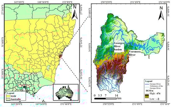
Figure 1.
The geographical location of the study area.
The digital elevation model (DEM) data for the basin were obtained from the Alaska Satellite Facility (ASF) Synthetic Aperture Radar database (https://search.asf.alaska.edu/, accessed on 10 May 2024), with a spatial resolution of 12.5 m × 12.5 m. Rainfall data (http://www.bom.gov.au/climate/data/, accessed on 10 May 2024), water level data (https://mhl.nsw.gov.au/, accessed on 10 May 2024), runoff discharge data (http://www.bom.gov.au/waterdata/, accessed on 10 May 2024), and river network data (http://www.bom.gov.au/water/geofabric, accessed on 10 May 2024) were used to develop the dynamic flood simulation model. This study utilized the latest 2021 Census data at the Statistical Area Level 1 (SA1) from the Australian Bureau of Statistics (https://www.abs.gov.au/census, accessed on 10 May 2024). Land use and land cover data were derived from 10 m resolution Sentinel-2 imagery (2023) available on the ESRI Living Atlas platform (https://livingatlas.arcgis.com/landcoverexplorer, accessed on 10 May 2024) to extract relevant indicator variables. Road network data were obtained from the New South Wales Government Spatial Portal (https://portal.spatial.nsw.gov.au/, accessed on 10 May 2024), and road density was calculated using a 50 m grid via line density analysis. These datasets were collectively employed to construct the integrated flood risk assessment model.
4. Materials and Methods
In this study, a flood risk assessment framework is constructed in the context of multi-return-period design floods. A coupled one-dimensional and two-dimensional (1D/2D) simulation model is used to analyze the spatial evolution of flood hazards and to extract high-resolution hazard indicators, as illustrated in Figure 2. The methodology comprises three main components: (1) the simulation of flood spatial evolution under multiple return-period scenarios within the basin; (2) the construction of an evaluation indicator system, which includes two primary categories—hazard intensity (disaster-inducing factors) and exposure vulnerability (disaster-bearing elements)—and ten secondary indicators, such as maximum inundation depth and maximum flood velocity; (3) flood risk assessment based on integrated weighting and TOPSIS, where subjective weights obtained via the TFAHP and objective weights derived from the EWM-CRITIC methods are integrated using a game-theoretic weighting model. The final flood risk levels for the floodplain areas in the Georges River Basin are evaluated using TOPSIS.
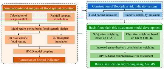
Figure 2.
Overall assessment system. The proposed framework enables dynamic and spatially explicit risk evaluation in support of sustainable floodplain management.
4.1. Flood Simulation Model for Basin Floodplains Under Multi-Return-Period Scenarios
During short-duration, high-intensity rainfall events, flood simulation in the basin involves three main components: one-dimensional flood routing in river channels driven by rainfall runoff, two-dimensional floodplain inundation caused by overbank flow, and a coupled 1D-2D simulation method. The simulation steps are as follows.
Step 1: Design of flood hydrographs under multi-return-period scenarios.
The historical annual maximum 24 h rainfall data recorded at the Glenfield Rainfall Station (33°98′ S, 150°91′ E) from 1984 to 2023 were compiled. The empirical frequency of rainfall was calculated, and a Pearson Type III distribution curve was fitted to derive the maximum 24 h rainfall corresponding to the 5-, 10-, 20-, 50-, and 100-year return periods. Based on the observed rainfall-runoff data from typical flood events, the unit hydrograph for the Georges River Basin was derived. Combined with the distributed rainfall after temporal allocation, the design flood hydrographs were subsequently developed.
Step 2: Simulation of one-dimensional river flood routing.
The hydrodynamic module of MIKE 11 was employed to conduct 1D flood routing simulations within the river channels, reproducing the temporal and spatial evolution of river floods and the corresponding water level rises. This process was used to identify overbank flow volumes and overflow locations. The simulation was governed by the Saint-Venant equations [31].
where A is the cross-sectional flow area (m2); Q is the discharge (m3/s); t and x represent the time (s) and distance (m), respectively; α is the momentum correction coefficient; g is the gravitational acceleration (m/s2); C is the Chezy coefficient; R is the hydraulic radius (m).
Step 3: Simulation of two-dimensional floodplain inundation.
When the river water level exceeds the left and right embankments, an unstructured triangular mesh, generated by terrain interpolation, is used as the computational grid. The overbank flow volumes calculated in Step 1 are applied as boundary conditions. MIKE 21 FM is then employed to simulate the 2D evolution of floodplain inundation. The simulation is governed by the Navier–Stokes equations [32].
where and are the depth-averaged velocity components in the x and y directions (m/s); t is the time (s); x and y are spatial coordinates (m); S is the source term; f is the Coriolis parameter; η is the bed elevation (m); d is the still water depth (m); h = η + d is the total water depth (m); ρ is the fluid density; ρ₀ is the reference density of the fluid (g/mL); g is the gravitational acceleration (m/s2); Sxx, Sxy, Syx, and Syy are the radiation stress components; us and vs are the flow velocities associated with the source term (m/s); Tᵢⱼ denotes the horizontal viscous stress; and Pa is the atmospheric pressure (Pa).
Step 4: Coupled 1D-2D flood simulation using MIKE FLOOD.
MIKE FLOOD was employed to perform the coupled simulation between the 1D river channel and the 2D floodplain. In this study, the 1D river channel crosses the 2D model domain, and flooding within the floodplain is primarily caused by river overbank flows. Therefore, lateral links were used to achieve the coupling between the 1D and 2D models. In the lateral link setup, the riverbanks in MIKE 11 are treated as weirs, and the lateral overflow discharge is calculated using the weir flow equation, as shown in Equation (6) [33].
where Q is the overflow discharge (m3/s); W is the weir width (m); Hw is the crest elevation of the weir (m); Hus and Hds are the upstream and downstream water levels, respectively (m); C is the weir flow coefficient; and k is the weir flow exponent, typically taken as 1.5.
4.2. Evaluation Indicator System
Based on the actual characteristics of the flood hazards reflected by the flood simulation results, and considering the operational feasibility of the study, ten evaluation indicators were ultimately selected, covering two main aspects: flood hazard intensity and exposure vulnerability. Among them, three indicators represent the intrinsic hazard intensity of flood events, while the actual flood risk is further influenced by seven indicators related to the vulnerability of the exposed elements, as shown in Table 1. The Australian Census data used in this study are based on Statistical Area Level 1 (SA1) units, which represent the smallest census division, each comprising between 200 and 800 people. A total of 584 SA1 units are located within the study area. Indicator data were calculated and spatially linked to the SA1 vector layer using the “join data” function in GIS, enabling the geographic distribution of socioeconomic data to be obtained.

Table 1.
Evaluation indicator system for flood risk in the floodplain areas of the Georges River Basin.
4.3. Flood Risk Assessment Based on Game Theory-Based Combined Weighting and TOPSIS
Since a single weighting model cannot simultaneously account for both the effective experience of decision-makers and the objective rationality of decisions, this study proposes an integrated subjective–objective combined weighting model. TFAHP is applied to calculate the subjective weights of indicators, and the improved EWM-CRITIC method is used to derive the objective weights. The optimal combination strategy of weights is then determined using an improved game-theoretic weighting model. TFAHP effectively integrates both data and expert judgments but heavily relies on the subjective experience of decision-makers [41]. The EWM, based on the information content carried by the data, avoids human subjectivity but is highly dependent on the availability and quality of the measurement data [42]. Game theory considers the differences and balance between subjective and objective weights, and the game-theoretic combined weighting model optimizes the integration of the two types of weights, thereby avoiding the bias that may arise from relying solely on a single weighting source [23].
4.3.1. Subjective Weight Calculation Based on the TFAHP
The FAHP retains the hierarchical structure and weighting calculation procedure of the traditional AHP but replaces the conventional 1–9 scale method with fuzzy numbers during pairwise comparisons of indicators. This substitution more effectively captures the uncertainty inherent in decision-making for complex problems. In this study, the TFAHP is adopted, where triangular fuzzy numbers, defined by three vertex values (minimum, maximum, and modal), are used to represent the degree of fuzziness in judgments. The TFAHP calculation procedure is detailed as follows.
Step 1: Pairwise comparison of indicators and the construction of the fuzzy matrix.
In a decision-making process involving n indicators, a triangular fuzzy decision matrix is constructed using triangular fuzzy numbers based on the pairwise comparisons among indicators at the same hierarchical level, as shown in Equation (7) [35]. Here, p represents the relative importance between indicators, consistent with the judgment values used in the traditional AHP method, while l and u represent the degree of fuzziness in the judgments.
Step 2: Calculation of the comprehensive evaluation index .
The importance of each indicator j is measured by calculating its comprehensive evaluation index [43].
Step 3: Pairwise comparison of comprehensive evaluation indices.
To obtain the indicator weights, pairwise comparisons of the comprehensive evaluation indices are performed. This process is based on the rules for the pairwise comparison of triangular fuzzy numbers. If and are triangular fuzzy numbers, the pairwise comparison between these two vectors is conducted according to Equation (9).
According to the rules for the pairwise comparison of fuzzy numbers, each comprehensive evaluation index is compared with the other n − 1 indices. The relative importance w′j of indicator j at the current hierarchical level is defined by Equation (10).
Step 4: Calculation of the subjective weights of indicators.
The fuzzy weight vector and the normalized weight vector of the indicators are obtained by calculating Equations (11) and (12).
4.3.2. Objective Weight Calculation Based on the Improved EWM-CRITIC Method
The CRITIC method calculates objective weights based on the amount of information an indicator carries, as determined by its variability and independence, using the objective values of each indicator. However, the traditional CRITIC method has several limitations. First, standard deviation is a dimensional quantity, which can lead to inconsistency when measuring data variability and thereby affect the accuracy of weight calculation. To address this, the coefficient of variation is introduced in this study to replace standard deviation as a measure of variability. Second, correlation coefficients contain positive or negative signs, yet the independence of indicators should reflect only the degree of correlation, regardless of direction. Therefore, the absolute values of the correlation coefficients are used to evaluate indicator independence. Third, standard deviation has a limited ability to describe data dispersion, especially when the data distribution is non-convex, and it performs poorly in representing uncertainty. In contrast, information entropy is more effective in measuring information uncertainty and dispersion. Hence, the entropy weight method (EWM) is integrated with the CRITIC method to improve the objectivity of weight determination. These three improvements compensate for the limitations of the original CRITIC method. The improved EWM-CRITIC method evaluates indicators from three dimensions—variability, independence, and dispersion—thus enabling a more rational and comprehensive objective weighting process. The steps for calculating indicator weights using the improved EWM-CRITIC method are as follows.
Step 1: Construction of the original decision matrix D and the normalized matrix .
In a decision-making problem involving m evaluation objects and n indicators, the original decision matrix D is first constructed. After performing dimensionless processing separately for positive and negative indicators, the normalized matrix is obtained [44].
Step 2: Calculation of information entropy ej to measure the dispersion of indicator j.
The normalized matrix is used to calculate the characteristic weight fij, based on which the information entropy ej of indicator j is determined using the EWM [45].
Step 3: Calculation of the coefficient of variation uj to measure the variability of indicator j.
where denotes the mean value of the attribute values for indicator j.
Step 4: Calculation of the quantitative coefficient ηj to measure the independence of criterion j.
Using the normalized matrix , the Pearson correlation coefficient is employed to quantify the correlation between indicator j and indicator k. The absolute values of the correlation coefficients are then used to calculate the independence coefficient ηj.
Step 5: Calculation of the information content Aj of indicator j.
Step 6: Calculation of the normalized objective weights Wo.
4.3.3. Indicator Weight Integration Based on the Improved Game-Theory Approach
Traditional game theory-based weighting methods lack a consistency verification process for identifying and adjusting the potential conflicts between weight vectors. Moreover, due to limitations in the objective function, the resulting combination coefficients may not always be positive. To address these issues, this study adopts an improved game-theoretic weighting approach to calculate the integrated weights. The specific computational steps are as follows.
Step 1: Consistency check of weight vectors derived from multiple weighting methods.
In the integration of l individual weighting methods for n indicators, the corresponding weight vectors are represented as shown in Equation (21). Taking l = 2 as an example, the consistency check is conducted by computing the distance function according to Equation (22).
where ws and wo represent the subjective and objective weights, respectively. When , the weights derived from the two methods are considered to meet the distance threshold and thus pass the consistency check. If , the individual weight results must be adjusted until the consistency condition is satisfied.
Step 2: Construction of the linear combination weighting function.
where αc denotes the combination coefficient for the weight vector.
Step 3: Construction of the optimized game-theoretic weighting model.
To determine the optimal combination coefficients, it is first necessary to establish an objective function for the model. The goal of the combination process is to minimize the deviation between the combined weight vector w and each individual weight vector wₖ [46].
To ensure that the combination coefficients are positive, a constraint is added to improve the objective function of the traditional game-theoretic model, resulting in an optimized formulation for calculating the combination coefficients.
The Lagrangian function is constructed to solve the above optimization model for the combination coefficients.
Assuming the existence of an extremum, partial derivatives are taken with respect to αc and λ, resulting in a system of partial differential equations.
By solving the system of partial differential equations, the optimal combination coefficient αc for the weight vector can be obtained.
Step 4: Calculation of optimal combined weights.
The normalized optimal combination coefficients αc* and the optimal integrated indicator weights W* are then obtained through calculation.
4.4. Integrated Floodplain Risk Assessment Under Multi-Return-Period Scenarios Based on TOPSIS
TOPSIS evaluates each alternative by calculating its relative distance to the ideal and anti-ideal solutions, thereby deriving a comprehensive score for each evaluation object. As a widely used method in multi-attribute decision-making (MADM), TOPSIS is favored for its simplicity and its ability to handle an unlimited number of alternatives and criteria [25]. Owing to its advantages in the MADM domain, TOPSIS has been extensively applied to flood risk assessment [47]. The calculation procedure is as follows.
Step 1: Construction of a game theory-based weighted decision matrix.
Step 2: Determination of the positive ideal solution S+ and negative ideal solution S− [48].
Step 3: Calculation of the Euclidean distances from each evaluation object to the positive and negative ideal solutions.
Step 4: Calculation of the relative closeness Ci of each evaluation object.
The value of Ci ranges from 0 to 1, with higher values indicating a closer proximity to the ideal solution.
5. Results and Discussion
5.1. Flood Inundation Under Multi-Return-Period Scenarios
The maximum inundation depths under multi-return-period flood scenarios are shown in Figure 3. The analysis reveals that water depth variations are most significant in the midstream Fairfield area and the downstream suburbs of Condell Park and Padstow. Among the five flood scenarios, the upstream riparian zones exhibit relatively minor changes in maximum inundation depth, while the midstream river bends show slight increases based on already inundated areas. In contrast, the downstream floodplain exhibits the most pronounced variation in maximum inundation depth across return periods. As the flood return period increases, the proportion of high-depth areas in the downstream region expands, and some locations experience a clear shift between inundated and non-inundated states. Therefore, greater attention should be given to the disaster impact and risk evolution in the downstream floodplain under extreme flood events.
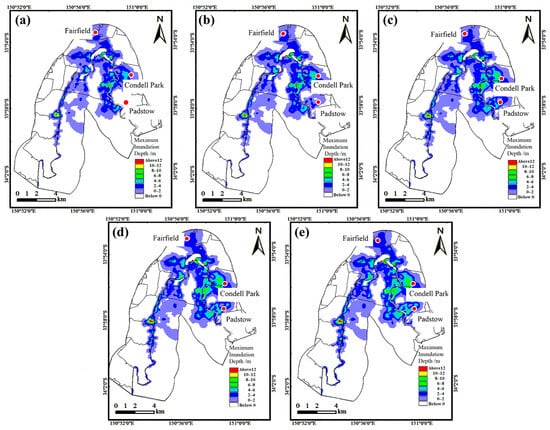
Figure 3.
Maximum inundation depth under multi-return-period flood scenarios: (a) 5-year return period; (b) 10-year return period; (c) 20-year return period; (d) 50-year return period; (e) 100-year return period.
The maximum inundation areas under the five designed flood scenarios are summarized in Table 2. Among them, the largest difference in inundation area is observed between the 5-year and 10-year return-period scenarios. As the return period increases, the additional inundated area gradually decreases. This indicates that once the flood magnitude reaches a certain threshold, further increases have a limited impact on the spatial extent of inundation. Instead, the severity of flood disasters becomes more prominently reflected in the depth of inundation.
Table 2.
Maximum inundation area under different design flood scenarios.
To ensure the spatial consistency and complete coverage of multi-source data within floodplain assessment units, all the socio-economic and surface-related indicators in this study were rasterized. For continuous variables, such as population density, road density, and per capita income, the inverse distance weighting (IDW) interpolation method was employed to convert point-based census data or statistical area data into continuous raster surfaces at a 30 m resolution. For categorical variables such as land use, the nearest neighbor interpolation method was used to preserve the spatial distribution characteristics of the original category attributes. The spatial extent of the interpolation covered the maximum inundation zone derived from all the return-period scenarios, ensuring that indicator data were complete and resolution-consistent for all grid cells within the flood risk assessment domain. This preprocessing step was essential for implementing a grid-based multi-indicator risk assessment and helped avoid spatial discontinuities caused by data heterogeneity.
5.2. Determination of Indicator Weights
The TFAHP is employed to determine the subjective weights of the evaluation indicators, while the EWM-CRITIC is used to calculate the objective weights. These two types of weights are then integrated using Equation (30) under the game-theoretic framework to obtain the comprehensive weights of each indicator, as shown in Table 3. Appendix A provides a detailed description of the calculation procedures for subjective weights, objective weights, and combined weights. With the increase in the flood return period, the objective weights of H1 (maximum inundation depth) and H2 (maximum flow velocity) exhibit a decreasing trend. This is attributed to the fact that both the maximum inundation depth and flow velocity generally increase with higher flood magnitudes in the study area, leading to a reduction in the variability of attribute values among the flood hazard indicators. Consequently, the amount of information carried by these indicators declines, resulting in lower objective weights. Across the five return-period scenarios, the indicators with the highest combined weights are the maximum inundation depth, maximum flood flow velocity, and population density. For instance, in the 5-year return-period scenario, the sum of their weights reaches 0.552, indicating that these three indicators play a dominant role in determining the overall flood risk. The remaining indicators, in descending order of weight, are the maximum inundation onset time, land use type, dependency ratio, and unemployment rate. Indicators with relatively low weights include the education level, per capita income, and road network density.
Table 3.
Weight results calculated by each assignment method.
5.3. Integrated Flood Risk Assessment Results for Basin Floodplains
Flood risk in this study was assessed using 50 m × 50 m grid cells as evaluation units; the relative closeness coefficient Ci to the ideal solution was calculated for all 57,163 spatial units within the study area. These values were then used to classify the flood hazard, vulnerability, and overall risk under five different return-period scenarios. The Jenks natural breaks classification method was employed to divide hazard, vulnerability, and integrated risk into five categories: low, moderate, moderate to high, high, and very high [49].
An analysis of flood hazard maps across multi-return periods indicates that the most notable difference between the 5-year and 10-year scenarios lies in the spatial extent of the hazard zones. For instance, areas such as northern Padstow, which are classified as non-hazardous under the 5-year scenario, fall within hazard zones under the 10-year scenario. As flood magnitude increases, the overall spatial extent of hazard zones tends to stabilize; however, the severity levels within these zones exhibit significant variation (Figure 4). These results suggest that under lower-magnitude flood events, priority should be given to monitoring and managing potentially at-risk areas that remain unaffected under mild conditions. In contrast, under high-magnitude floods, greater focus should be placed on existing inundated areas with intensifying hazard severity. This underscores the importance of strengthening flood protection standards to enhance disaster prevention and mitigation capacity.
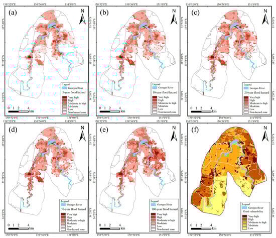
Figure 4.
Flood hazard and vulnerability maps under multi-return-period scenarios: (a) 5-year flood hazard; (b) 10-year flood hazard; (c) 20-year flood hazard; (d) 50-year flood hazard; (e) 100-year flood hazard; (f) flood vulnerability. The expansion of high-hazard zones in downstream areas as the flood return period increases.
Since flood vulnerability is solely related to the natural environmental characteristics and socio-economic attributes of a region, it is considered an inherent property of the study area, independent of the occurrence or severity of flood events. In this study, the computed weights of the vulnerability indicators differ only at a magnitude of 0.001, suggesting that flood vulnerability across the study area remains consistent under multi-return-period scenarios. Among the vulnerability indicators, population density and land use type have the highest weight proportions and play a decisive role in determining social vulnerability. The right bank areas of the upstream and downstream rivers, such as Holsworthy–Wattle Grove, are predominantly covered by vegetation, which enhances their disaster resilience and results in lower social vulnerability. In contrast, the left bank and midstream right bank regions, characterized by dense residential and built-up areas, exhibit generally higher levels of social vulnerability, although variations still exist among specific zones due to differences in other indicators. The analysis confirms that the flood vulnerability map generated using the integrated weighting–TOPSIS method is reasonable and reliable.
The flood risk maps of the basin under multiple return-period scenarios are shown in Figure 5, and Table 4 presents the corresponding proportions of each risk level. As the return period increases, the proportion of areas classified as moderate-to-high risk or above shows a clear upward trend. Compared to the 5-year return-period scenario, the 100-year scenario exhibits an increase in the proportion of moderate-to-high risk areas from 26.3% to 37.0%, high-risk areas from 9.9% to 15.8%, and very-high-risk areas from 0.9% to 2.7%. Conversely, the proportion of moderate- and low-risk areas decreases, with moderate-risk areas declining from 47.2% to 39.5%, and low-risk areas declining from 15.6% to 5.0%. These results reflect a consistent increase in the overall flood risk levels across the floodplain under longer return-period scenarios.
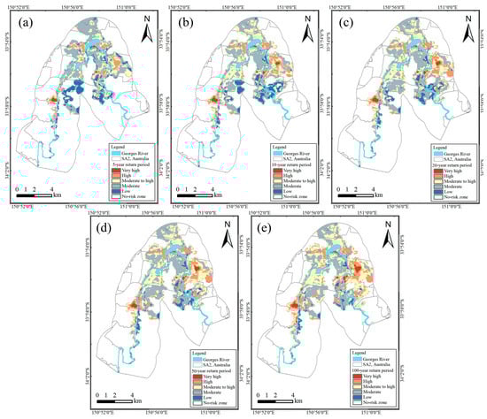
Figure 5.
Flood risk maps under multi-return-period scenarios: (a) 5-year; (b) 10-year; (c) 20-year; (d) 50-year; (e) 100-year. The maps illustrate a clear expansion of high and very high flood risk zones, particularly in the downstream floodplain as the return period increases. This highlights the importance of incorporating multi-scenario analysis in flood risk management and adaptive urban planning.
Table 4.
Area proportions of different flood risk levels under multi-return-period scenarios.
Since conventional flood risk maps do not intuitively capture the variations in risk across different flood scenarios, ArcGIS was employed to conduct cross-mapping for a comparative analysis of flood risk classifications under multiple return periods. Taking the 5-year design flood scenario as the baseline, cross-maps were generated with the 10-, 20-, 50-, and 100-year return-period scenarios. Risk levels are categorized from 1 to 5, representing low, moderate, moderate to high, high, and very high, respectively. For instance, a code such as “12” indicates that an area classified as low risk under the 5-year scenario is assessed as moderate risk under another scenario. The cross-mapping results are presented in Figure 6.
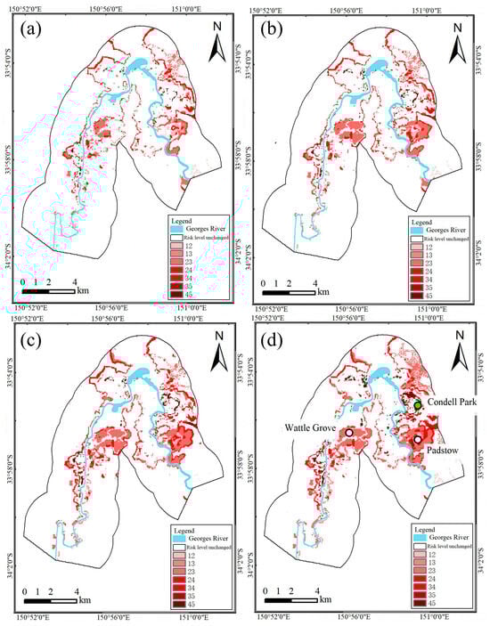
Figure 6.
Cross-mapping of flood risk under multi-return-period scenarios: (a) 5- and 10-year; (b) 5- and 20-year; (c) 5- and 50-year; (d) 5- and 100-year.
The analysis of the cross-mapping results indicates that flood risk levels across the floodplain generally increase with longer flood return periods. Significant changes in risk classification are observed in the middle and lower reaches of the river, particularly in areas such as Wattle Grove in the midstream and Condell Park and Padstow in the downstream. The area-based statistics of regions with rising risk levels show that, compared to the 5-year design flood, the proportions of areas experiencing risk level increases under the 10-, 20-, 50-, and 100-year scenarios are 8.82%, 11.47%, 13.65%, and 16.55%, respectively.
5.4. Flood Risk Validation
Obtaining accurate and high-resolution ground-truth data for flood disasters remains a persistent challenge in flood risk studies. This difficulty is particularly pronounced in non-prioritized monitoring basins or regions, where systematic records such as historical inundation maps or observed water depths are often unavailable, thereby limiting the validation of the simulation models. Consequently, event-driven data sources such as social media and official announcements have emerged as practical and cost-effective alternatives [50,51]. To verify the accuracy of the proposed flood risk assessment model, descriptive information on flood inundation characteristics within the study area was collected from government websites, news media, and social media platforms. According to the official Georges River website (https://georgesriver.org.au/, accessed on 15 June 2024), the flood events that occurred in February 2020, March 2022, and June 2022 were equivalent in magnitude to a 1-in-20-year return-period flood. Therefore, social media data from these three events were compiled to construct a historical flood impact validation dataset for the Georges River Basin, as summarized in Table 5.
Table 5.
Disaster information network validation dataset for the Georges River Basin based on social media data.
When compared with the risk levels indicated on the 1-in-20-year flood risk map, the actual disaster events closely correspond to the assessed risk levels. This demonstrates that the proposed game-theoretic combination weighting–TOPSIS risk assessment model is capable of effectively identifying the major flood-prone risk areas in the Georges River Basin, thereby validating the model’s effectiveness and reliability.
5.5. Uncertainties in MIKE Model Applications
Although the MIKE model is a well-established physics-based simulation tool widely applied in flood modeling studies, its outputs are still subject to uncertainties arising from model structural simplifications, the spatial resolution of terrain data, and parameter settings such as uniform surface roughness. First, the spatial resolution of the digital elevation model (DEM) directly influences the delineation of the inundation boundaries in low-lying areas; inaccuracies can result in significant errors in flood extent. Second, parameters such as Manning’s roughness coefficient greatly affect flood propagation velocity and water depth distribution; improper local settings may distort simulation results. Third, the temporal distribution of rainfall intensity plays a critical role in determining inflow volume, and variations in peak timing within rainfall design assumptions can result in significant differences in inundation patterns.
These uncertainties primarily stem from external factors such as topographic data accuracy, parameter calibration, and future climate variability. In this study, model parameters were calibrated using observed water levels and inundation extents from a representative historical flood event. Key parameters, including Manning’s roughness coefficients, were assigned based on land use types and adjusted locally to ensure simulation reliability. Therefore, under the current data conditions, the uncertainties related to model structure and parameterization have been effectively controlled.
However, this study did not incorporate future climate scenarios or account for changes in hydraulic infrastructure systems (e.g., levee breaches and gate operations), which could significantly influence flood dynamics and risk distribution under extreme conditions. These aspects remain beyond the scope of quantification given the current data limitations. Future research could extend the existing framework by integrating land surface changes, extreme rainfall forecasts, and dynamic engineering system responses to enhance model adaptability and early warning capabilities.
5.6. Floodplain Risk Management Strategies
Incorporating multiple return-period scenarios not only enables a more comprehensive understanding of how flood risk evolves with event magnitude but also supports graded floodplain zoning and the development of adaptive management strategies. Nandam and Patel [52], for instance, compared floods with 50-, 100-, and 250-year return periods and found that as the return period increases, high-risk areas tend to expand while low-risk areas shrink, highlighting the significant influence of flood magnitude on risk management. The findings of this study similarly reveal that under lower return-period scenarios, flood-prone areas experience frequent events but generally exhibit lower risk levels, with manageable impacts. Based on the floodplain risk assessment under multiple return-period scenarios, three targeted and practically applicable management strategies are proposed.
First, structural flood control measures should be prioritized in densely populated downstream areas. Integrated river management should be implemented to enhance flood conveyance capacity through channel dredging, thereby preventing an abnormal water level rise caused by local sedimentation. Reinforcing riverbanks in critical zones can help mitigate flood overtopping. Flood protection standards in key floodplain areas should be upgraded by introducing floodwalls and temporary or mobile barriers to enhance the resilience of communities and buildings. In addition, greater emphasis should be placed on nature-based solutions, such as establishing flood retention zones and storage basins to balance retention and discharge, promoting ecological restoration, and increasing vegetation coverage to support ecosystem-based disaster mitigation.
Second, non-structural approaches that preserve natural buffers are more suitable for upstream areas to reduce floodplain vulnerability. For newly affected zones under high return-period flood scenarios, limited resident exposure may impair risk perception; thus, flood awareness and public education should be strengthened to improve preparedness and enhance public trust in flood management. In regions with low per capita income and high unemployment rates, additional financial support is needed to enhance disaster resilience through government-provided flood protection supplies and emergency reserves. Evacuation priority should be determined based on the difficulty of evacuation and rescue operations. Areas with high dependency ratios (e.g., high densities of elderly or children) and limited road accessibility should be prioritized. Evacuation strategies should be clearly defined, including evacuation modes, phased implementation, and route planning, to ensure an orderly emergency response. Moreover, early warning and response systems for floods should account for the nonlinear spatial expansion of risk and adopt dynamic alert levels accordingly.
Finally, it is essential to control development and population expansion within floodplains in order to reduce the risks associated with land use and population density. A comprehensive floodplain safety management plan should be developed, incorporating hierarchical and zoned flood control strategies. In high-risk areas that are inundated across all return-period scenarios, residents should be relocated through organized measures such as property acquisition and resettlement programs to restore floodplain space to the natural flow. In moderate- and low-risk areas with potential inundation, population and asset growth should be regulated. Infrastructure unrelated to flood control and riverbank development should be restricted, and the layout of urban, rural, and residential settlements should be planned to avoid flood-prone zones as much as possible.
5.7. Limitations
Firstly, under the backdrop of global climate change, there is increasing uncertainty associated with extreme rainfall and flood hazards. As noted by Zhu et al. [53], depending on the climate model used, the 20-year return-period daily rainfall in the mid-to-low latitudes of southeastern coastal Australia may increase by approximately 10–37%, potentially resulting in proportional increases in runoff. This study designs flood scenarios based on historical rainfall and runoff data but lacks an analysis of flood risk changes under future climate extremes, which should be further explored in future research. Secondly, the flood risk assessment in this study is based on five return-period scenarios, but the simulations did not incorporate additional hydraulic elements. Future work should consider complex conditions such as levee breaches and dam overtopping, as well as variable riverbank heights and the operational states of hydraulic structures, to enable more diverse and refined scenario analysis. Thirdly, although the use of event-driven data sources such as social media and government reports provides a practical and cost-effective alternative for model validation in non-prioritized monitoring basins or regions, this approach still has certain limitations. On the one hand, social media data are often unevenly distributed, subjective, and lack quantitative standards. On the other hand, official and media sources may overlook mildly affected or peripheral areas, introducing bias in the validation dataset. Looking ahead, the validation framework can be further enhanced by incorporating water extent maps derived from synthetic aperture radar (SAR) data (e.g., Sentinel-1), crowdsourced disaster platforms (e.g., FloodMap), insurance claims data, and in situ hydrological observations. These sources can improve the resolution, objectivity, and spatial completeness of the validation dataset, thereby increasing the robustness of the proposed model framework. Lastly, another important aspect that warrants further discussion is the treatment of vulnerability as a static component. While the flood hazard is dynamically simulated across multiple return periods, the vulnerability assessment relies solely on current socio-economic conditions. This approach overlooks the potential evolution of social vulnerability over time due to factors such as population growth, urban development, and changes in infrastructure or land use. Incorporating dynamic vulnerability projections would provide a more realistic and forward-looking assessment of flood risk. It is recommended that future studies explore methods for integrating temporal changes in exposure and adaptive capacity to enhance the robustness of risk evaluations.
6. Conclusions
This study addresses the limitations in conventional multi-criteria flood risk assessment methods, including the narrow focus on single-scenario analysis, the lack of refined hazard indicators, and the challenge of balancing subjective expert judgment with objective data-driven insights. A comprehensive flood risk assessment framework was proposed based on multi-return-period flood scenarios, refined hydrodynamic hazard simulation, and a game-theoretic combination weighting–TOPSIS model. The Georges River Basin in Australia was selected as the case study to demonstrate the applicability and validity of the proposed approach.
(1) The study first established five design flood scenarios corresponding to 5-, 10-, 20-, 50-, and 100-year return periods using 39 years of historical rainfall data from the Glenfield station. A synthetic flood hydrograph was generated using the unit hydrograph method derived from a typical flood event in February 2020, enabling scenario-based modeling even in regions lacking empirical runoff parameters.
(2) To overcome the static limitations of traditional hazard indicators, a coupled 1D/2D hydrodynamic model was developed using MIKE11 and MIKE21, which effectively simulated the flood evolution process, inundation extent, and dynamics across the basin. Key hazard indicators (maximum inundation depth, maximum flow velocity, and maximum time to peak inundation) were extracted, providing a dynamic and spatially explicit characterization of flood hazards under multiple scenarios. The analysis revealed that while the flood extent varies significantly under lower-magnitude events, differences in the flood depth dominate as the return period increases.
(3) The study further constructed a comprehensive risk assessment index system incorporating three hazard indicators and seven vulnerability indicators, covering exposure characteristics, socio-economic resilience, and evacuation difficulty. Subjective weights were derived via the TFAHP and objective weights via the EWM-CRITIC, which were then integrated using a game-theoretic optimization model to determine the final combined weights. TOPSIS was applied for a multi-criteria risk synthesis across 50 m × 50 m grid cells. The results show a clear trend of increasing high-risk zones with an increasing return period: compared to the 5-year scenario, the proportion of regions with elevated risk levels increased by 8.82%, 11.47%, 13.65%, and 16.55% under the 10-, 20-, 50-, and 100-year scenarios, respectively.
Validation using historical disaster records confirmed the spatial consistency between modeled high-risk zones and actual flood-affected areas, supporting the reliability and applicability of the proposed framework. Based on the floodplain risk assessment results under multiple return-period scenarios, targeted and practically valuable risk management strategies are proposed for graded and zoned flood control.
In addition to further advancing methodological development, the proposed framework offers valuable insights for a wide range of stakeholders. Specifically, the findings can support data-driven flood risk management strategies that benefit policymakers, urban planners, and emergency services, while also empowering local communities to better prepare for and respond to disaster risks. By promoting more inclusive, resilient, and sustainable urban development, this work directly contributes to the achievement of SDG 11: Sustainable Cities and Communities.
Author Contributions
Conceptualization, X.R. and H.S.; methodology, Q.Y., W.S. and J.W.; visualization, X.R. and H.S.; formal analysis, X.R. and W.S.; writing—original draft preparation, X.R., Q.Y. and H.S.; writing—review and editing, W.S. and J.W.; data curation, H.S. and J.W.; supervision, X.R., H.S. and W.S.; project administration, X.R. All authors have read and agreed to the published version of the manuscript.
Funding
This research was funded by the Natural Science Foundation of Qingdao Municipality, grant number 23-2-1-61-zyyd-jch, National Natural Science Foundation of China, grant number 52071307, and the Key R & D projects of Shandong Province, grant number 2020CXGC010702.
Institutional Review Board Statement
Not applicable.
Informed Consent Statement
Not applicable.
Data Availability Statement
The original contributions presented in this study are included in the article. Further inquiries can be directed to the corresponding author(s).
Conflicts of Interest
The authors declare no conflicts of interest.
Appendix A
Table A1.
Subjective weights of flood hazard indicators calculated using the TFAHP.
Table A1.
Subjective weights of flood hazard indicators calculated using the TFAHP.
| H | H1 | H2 | H3 | wH | w | ||
|---|---|---|---|---|---|---|---|
| H1 | (1, 1, 1) | (1.2, 1.8, 2.5) | (1.5, 3, 4) | (0.25, 0.52, 0.99) | 0.53 | 0.33 | |
| H2 | (0.4, 0.56, 0.83) | (1, 1, 1) | (0.8, 2, 2.5) | (0.15, 0.32, 0.57) | 0.33 | 0.19 | |
| H3 | (0.25, 0.33, 0.67) | (0.4, 0.5, 1.25) | (1, 1, 1) | (0.11, 0.16, 0.39) | 0.15 | 0.09 | |
Table A2.
Objective weights of indicators under the 5-year return-period flood scenario.
Table A2.
Objective weights of indicators under the 5-year return-period flood scenario.
| Risk Indicators | H1 | H2 | H3 | V1 | V2 | V3 | V4 | V5 | V6 | V7 |
|---|---|---|---|---|---|---|---|---|---|---|
| Information entropy ej | 1.13 | 2.20 | 0.95 | 1.18 | 1.70 | 1.01 | 1.18 | 1.21 | 1.02 | 1.01 |
| Coefficient of variation uj | 2.34 | 3.16 | 1.53 | 0.60 | 1.68 | 0.42 | 0.64 | 2.20 | 0.90 | 0.13 |
| Independence coefficient ηj | 6.57 | 6.75 | 6.85 | 6.49 | 6.59 | 6.61 | 7.39 | 7.14 | 6.70 | 7.58 |
| Information content Aj | 0.53 | 0.79 | 0.36 | 0.27 | 0.51 | 0.22 | 0.25 | 0.48 | 0.29 | 0.15 |
| Objective weight wj | 0.14 | 0.21 | 0.09 | 0.07 | 0.13 | 0.06 | 0.06 | 0.12 | 0.08 | 0.04 |
Table A3.
Optimal combined weights of indicators calculated based on the improved game-theoretic approach.
Table A3.
Optimal combined weights of indicators calculated based on the improved game-theoretic approach.
| Multi-Return-Period Scenarios | d(ws,wo) | wswsT | wowsT | wswoT | wowoT | αs | αo | α*s | α*o |
|---|---|---|---|---|---|---|---|---|---|
| 5-year return period | 0.154 | 0.180 | 0.128 | 0.128 | 0.123 | 1.953 | 1.595 | 0.551 | 0.449 |
| 10-year return period | 0.157 | 0.180 | 0.126 | 0.126 | 0.122 | 1.975 | 1.601 | 0.552 | 0.448 |
| 20-year return period | 0.164 | 0.180 | 0.124 | 0.124 | 0.122 | 1.994 | 1.613 | 0.553 | 0.447 |
| 50-year return period | 0.164 | 0.180 | 0.124 | 0.124 | 0.122 | 1.994 | 1.613 | 0.553 | 0.447 |
| 100-year return period | 0.171 | 0.180 | 0.121 | 0.121 | 0.120 | 2.025 | 1.626 | 0.555 | 0.445 |
References
- IPCC Sixth Assessment Report. Available online: https://www.ipcc.ch/report/ar6/wg2/ (accessed on 15 June 2025).
- Isia, I.; Hadibarata, T.; Hapsari, R.I.; Jusoh, M.N.H.; Bhattacharjya, R.K.; Shahedan, N.F. Assessing Social Vulnerability to Flood Hazards: A Case Study of Sarawak’ s Divisions. Int. J. Disast. Risk Re. 2023, 97, 104052. [Google Scholar] [CrossRef]
- Herold, N.; Downes, S.M.; Gross, M.H.; Ji, F.; Nishant, N.; Macadam, I.; Ridder, N.N.; Beyer, K. Projected Changes in the Frequency of Climate Extremes over Southeast Australia. Environ. Res. Commun. 2021, 3, 011001. [Google Scholar] [CrossRef]
- Alabbad, Y.; Demir, I. Comprehensive Flood Vulnerability Analysis in Urban Communities: Iowa Case Study. Int. J. Disaster Risk Reduct. 2022, 74, 102955. [Google Scholar] [CrossRef]
- Solaimani, K.; Shokrian, F.; Darvishi, S. An Assessment of the Integrated Multi-Criteria and New Models Efficiency in Watershed Flood Mapping. Water Resour. 2023, 37, 403–425. [Google Scholar] [CrossRef]
- Mishra, A.; Mukherjee, S.; Merz, B.; Singh, V.P.; Wright, D.B.; Villarini, G.; Paul, S.; Kumar, D.N.; Khedun, C.P.; Niyogi, D.; et al. An Overview of Flood Concepts, Challenges, and Future Directions. J. Hydrol. Eng. 2022, 27, 03122001. [Google Scholar] [CrossRef]
- Wu, M.; Chen, M.; Chen, G.; Zheng, D.; Zhao, Y.; Wei, X.; Xin, Y. Research on Methodology for Assessing Social Vulnerability to Urban Flooding: A Case Study in China. J. Hydrol. 2024, 645, 132177. [Google Scholar] [CrossRef]
- Luo, Z.; Tian, J.; Zeng, J.; Pilla, F. Flood Risk Evaluation of the Coastal City by the EWM-TOPSIS and Machine Learning Hybrid Method. Int. J. Disaster Risk Reduct. 2024, 106, 104435. [Google Scholar] [CrossRef]
- Lin, W.; Sun, Y.; Nijhuis, S.; Wang, Z. Scenario-Based Flood Risk Assessment for Urbanizing Deltas Using Future Land-Use Simulation (FLUS): Guangzhou Metropolitan Area as a Case Study. Sci. Total Environ. 2020, 739, 139899. [Google Scholar] [CrossRef]
- Karami, M.; Abedi Koupai, J.; Gohari, S.A. Integration of SWAT, SDSM, AHP, and TOPSIS to Detect Flood-Prone Areas. Nat. Hazards. 2024, 120, 6307–6325. [Google Scholar] [CrossRef]
- Huthoff, F.; Remo, J.W.F.; Pinter, N. Improving Flood Preparedness Using Hydrodynamic Levee-breach and Inundation Modelling: Middle Mississippi River, USA. J. Flood Risk Manag. 2015, 8, 2–18. [Google Scholar] [CrossRef]
- Farooq, U.; Taha Bakheit Taha, A.; Tian, F.; Yuan, X.; Ajmal, M.; Ullah, I.; Ahmad, M. Flood Modelling and Risk Analysis of Cinan Feizuo Flood Protection Area, Huaihe River Basin. Atmosphere. 2023, 14, 678. [Google Scholar] [CrossRef]
- Mudashiru, R.B.; Sabtu, N.; Abdullah, R.; Saleh, A.; Abustan, I. Optimality of Flood Influencing Factors for Flood Hazard Mapping: An Evaluation of Two Multi-Criteria Decision-Making Methods. J. Hydrol. 2022, 612, 128055. [Google Scholar] [CrossRef]
- Xu, H.; Ma, C.; Lian, J.; Xu, K.; Chaima, E. Urban Flooding Risk Assessment Based on an Integrated k-Means Cluster Algorithm and Improved Entropy Weight Method in the Region of Haikou, China. J. Hydrol. 2018, 563, 975–986. [Google Scholar] [CrossRef]
- Wu, J.; Chen, X.; Lu, J. Assessment of Long and Short-Term Flood Risk Using the Multi-Criteria Analysis Model with the AHP-Entropy Method in Poyang Lake Basin. Int. J. Disaster Risk Reduct. 2022, 75, 102968. [Google Scholar] [CrossRef]
- Ajjur, S.B.; Al-Ghamdi, S.G. Exploring Urban Growth-Climate Change-Flood Risk Nexus in Fast Growing Cities. Sci. Rep. 2022, 12, 12265. [Google Scholar] [CrossRef]
- Zhang, T.; Wang, D.; Lu, Y. Machine Learning-Enabled Regional Multi-Hazards Risk Assessment Considering Social Vulnerability. Sci. Rep. 2023, 13, 13405. [Google Scholar] [CrossRef]
- Gizzi, F.T.; Bovolin, V.; Villani, P.; Potenza, M.R.; Voria, S.; Amodio, A.M. Rewinding the Tape: Documentary Heritage to (Re)Discover “Lost” Natural Hazards—Evidence and Inferences from Southern Italy. Sustainability 2024, 16, 2789. [Google Scholar] [CrossRef]
- Li, W.; Jiang, R.; Wu, H.; Xie, J.; Zhao, Y.; Song, Y.; Li, F. A System Dynamics Model of Urban Rainstorm and Flood Resilience to Achieve the Sustainable Development Goals. Sustain. Cities Soc. 2023, 96, 104631. [Google Scholar] [CrossRef]
- Ruan, X.; Sun, H.; Shou, W.; Wang, J. The Impact of Climate Change and Urbanization on Compound Flood Risks in Coastal Areas: A Comprehensive Review of Methods. Appl. Sci. 2024, 14, 10019. [Google Scholar] [CrossRef]
- Chen, X.; Zhang, H.; Chen, W.; Huang, G. Urbanization and Climate Change Impacts on Future Flood Risk in the Pearl River Delta under Shared Socioeconomic Pathways. Sci. Total Environ. 2021, 762, 143144. [Google Scholar] [CrossRef]
- Vanolya, N.M.; Jelokhani-Niaraki, M. The Use of Subjective-Objective Weights in GIS-Based Multi-Criteria Decision Analysis for Flood Hazard Assessment: A Case Study in Mazandaran, Iran. GeoJournal. 2021, 86, 379–398. [Google Scholar] [CrossRef]
- Peng, J.; Zhang, J. Urban Flooding Risk Assessment Based on GIS-Game Theory Combination Weight: A Case Study of Zhengzhou City. Int. J. Disaster Risk Reduct. 2022, 77, 103080. [Google Scholar] [CrossRef]
- Guo, G.; Gao, Y.; Sun, K. Whether Higher Risk Indicates Severe Loss in the Flood Disaster Assessment: A Comparative Analysis in the Hubei Province of Central China. J. Hydrol. Reg. Stud. 2024, 56, 102002. [Google Scholar] [CrossRef]
- Lu, P.; Sun, Y.; Steffen, N. Scenario-Based Performance Assessment of Green-Grey-Blue Infrastructure for Flood-Resilient Spatial Solution: A Case Study of Pazhou, Guangzhou, Greater Bay Area. Landsc. Urban Plan. 2023, 238, 104804. [Google Scholar] [CrossRef]
- Ji, J.; Chen, J. Urban Flood Resilience Assessment Using RAGA-PP and KL-TOPSIS Model Based on PSR Framework: A Case Study of Jiangsu Province, China. Water Sci. Technol. 2022, 86, 3264–3280. [Google Scholar] [CrossRef] [PubMed]
- Yuan, D.; Wang, H.; Wang, C.; Yan, C.; Xu, L.; Zhang, C.; Wang, J.; Kou, Y. Characteristics of Urban Flood Resilience Evolution and Analysis of Influencing Factors: A Case Study of Yingtan City, China. Water 2024, 16, 834. [Google Scholar] [CrossRef]
- Xu, W.; Cai, X.; Yu, Q.; Proverbs, D.; Xia, T. Modelling Trends in Urban Flood Resilience towards Improving the Adaptability of Cities. Water 2024, 16, 1614. [Google Scholar] [CrossRef]
- Giacon, A.J.; Da Silva, A.M. Flood Susceptibility Mapping in River Basins: A Risk Analysis Using AHP-TOPISIS-2 N Support and Vector Machine. Nat. Hazards. 2025, 121, 3239–3266. [Google Scholar] [CrossRef]
- Pathan, A.I.; Girish Agnihotri, P.; Said, S.; Patel, D. AHP and TOPSIS Based Flood Risk Assessment-a Case Study of the Navsari City, Gujarat, India. Environ. Monit. Assess. 2022, 194, 509. [Google Scholar] [CrossRef]
- Cea, L.; Costabile, P. Flood Risk in Urban Areas: Modelling, Management and Adaptation to Climate Change. A Review. Hydrology 2022, 9, 50. [Google Scholar] [CrossRef]
- Zhang, W.; Zhang, X.; Liu, Y.; Tang, W.; Xu, J.; Fu, Z. Assessment of Flood Inundation by Coupled 1d/2d Hydrodynamic Modeling: A Case Study in Mountainous Watersheds along the Coast of Southeast China. Water 2020, 12, 822. [Google Scholar] [CrossRef]
- DHI. Available online: https://www.dhigroup.com/ (accessed on 1 March 2025).
- Chakraborty, S.; Mukhopadhyay, S. Assessing Flood Risk Using Analytical Hierarchy Process (AHP) and Geographical Information System (GIS): Application in Coochbehar District of West Bengal, India. Nat. Hazards. 2019, 99, 247–274. [Google Scholar] [CrossRef]
- Sun, H.; Yu, Q.; Wang, X.; Zhang, X.; Ruan, X. Exploring Sustainable Watershed Flood Risks Management: An Innovative TFAHP-TOPSIS Methodology in the Georges River Basin, Australia. Int. J. Disaster Risk Reduct. 2024, 110, 104626. [Google Scholar] [CrossRef]
- Hsiao, S.C.; Chiang, W.S.; Jang, J.H.; Wu, H.L.; Lu, W.S.; Chen, W.B.; Wu, Y.T. Flood Risk Influenced by the Compound Effect of Storm Surge and Rainfall under Climate Change for Low-Lying Coastal Areas. Sci. Total Environ. 2021, 764, 144439. [Google Scholar] [CrossRef] [PubMed]
- Hinojos, S.; McPhillips, L.; Stempel, P.; Grady, C. Social and Environmental Vulnerability to Flooding: Investigating Cross-Scale Hypotheses. Appl. Geogr. 2023, 157, 103017. [Google Scholar] [CrossRef]
- Mruksirisuk, P.; Thanvisitthpon, N.; Pholkern, K.; Garshasbi, D.; Saguansap, P. Flood Vulnerability Assessment of Thailand’s Flood-Prone Pathum Thani Province and Vulnerability Mitigation Strategies. J. Environ. Manag. 2023, 347, 119276. [Google Scholar] [CrossRef]
- Asbridge, E.F.; Low Choy, D.; Mackey, B.; Serrao-Neumann, S.; Taygfeld, P.; Rogers, K. Coastal Flood Risk within a Peri-Urban Area: SUSSEX Inlet District, SE Australia. Nat. Hazards. 2021, 109, 999–1026. [Google Scholar] [CrossRef]
- Sun, R.; Gong, Z.; Gao, G.; Shah, A.A. Comparative Analysis of Multi-Criteria Decision-Making Methods for Flood Disaster Risk in the Yangtze River Delta. Int. J. Disaster Risk Reduc. 2020, 51, 101768. [Google Scholar] [CrossRef]
- Xie, W.; Meng, Q. An Integrated PCA-AHP Method to Assess Urban Social Vulnerability to Sea Level Rise Risks in Tampa. Florida. Sustainability 2023, 15, 2400. [Google Scholar] [CrossRef]
- Cao, F.; Wang, H.; Zhang, C.; Kong, W. Social Vulnerability Evaluation of Natural Disasters and Its Spatiotemporal Evolution in Zhejiang Province. China. Sustainability 2023, 15, 6400. [Google Scholar] [CrossRef]
- Ma, Z.; Liu, J.; Chien, S.I.J.; Hu, X.; Shao, Y. Identifying Critical Stations Affecting Vulnerability of a Metro Network Considering Passenger Flow and Cascading Failure: Case of Xi’an Metro in China. ASCE-ASME J. Risk Uncertain. Eng. Syst. Part A: Civ. Eng. 2023, 9, 04023014. [Google Scholar] [CrossRef]
- Zhao, H.; Zhong, M.; Li, L.; Safdar, M.; Zhang, Z. A Comprehensive Evaluation Method for Planning and Design of Self-Sufficient Wind Power Energy Systems at Ports. Sustainability 2023, 15, 16189. [Google Scholar] [CrossRef]
- Lu, X.; Ren, S.; Cui, Y.; Yin, X.; Chen, X.; Zhang, Y.; Moghtaderi, B. A Novel Site Selection Approach for Co-Location of Petrol-Hydrogen Fueling Stations Using a Game Theory-Based Multi-Criteria Decision-Making Model. Int. J. Hydrog. Energy. 2025, 106, 1443–1461. [Google Scholar] [CrossRef]
- Zheng, W.; Xu, S.; Wang, Z. Fuzzy Comprehensive Evaluation of Collapse Risk in Mountain Tunnels Based on Game Theory. Appl. Sci. 2024, 14, 5163. [Google Scholar] [CrossRef]
- Rafiei-Sardooi, E.; Azareh, A.; Choubin, B.; Mosavi, A.H.; Clague, J.J. Evaluating Urban Flood Risk Using Hybrid Method of TOPSIS and Machine Learning. Int. J. Disaster Risk Reduct. 2021, 66, 102614. [Google Scholar] [CrossRef]
- Kang, H.Y.; Chae, S.T.; Chung, E.S. Quantifying Medium-Sized City Flood Vulnerability Due to Climate Change Using Multi-Criteria Decision-Making Techniques: Case of Republic of Korea. Sustainability 2023, 15, 16061. [Google Scholar] [CrossRef]
- Jenks, G.F.; Caspalla, F.C. Error on Choroplethic Maps: Definition, Measurement, Reduction. Ann. Assoc. Am. Geogr. 1971, 61, 217–244. [Google Scholar] [CrossRef]
- Smith, L.; Liang, Q.; James, P.; Lin, W. Assessing the Utility of Social Media as a Data Source for Flood Risk Management Using a Real-Time Modelling Framework. J. Flood Risk Manag. 2017, 10, 370–380. [Google Scholar] [CrossRef]
- Joyce, J.; Arthur, R.; Fu, G.; Bialkowski, A.; Williams, H. Using Social Sensing to Validate Flood Risk Modelling in England. In AI 2023: Advances in Artificial Intelligence; Liu, T., Webb, G., Yue, L., Wang, D., Eds.; AI 2023. Lecture Notes in Computer Science; Springer: Singapore, 2024; Volume 14472. [Google Scholar] [CrossRef]
- Nandam, V.; Patel, P.L. Comprehensive Analysis of Data Aggregation Techniques for Flood Vulnerability and Bivariate Flood Risk Mapping of a Coastal Urban Floodplain. Int. J. Disaster Risk Reduct. 2025, 119, 105330. [Google Scholar] [CrossRef]
- Zhu, W.; Wang, X.H.; Peirson, W.; Salcedo-Castro, J. Assessment of Model Projections of Climate-change Induced Extreme Storms on the South-east Coast of Australia. Int. J. Climatol. 2024, 44, 2139–2159. [Google Scholar] [CrossRef]
Disclaimer/Publisher’s Note: The statements, opinions and data contained in all publications are solely those of the individual author(s) and contributor(s) and not of MDPI and/or the editor(s). MDPI and/or the editor(s) disclaim responsibility for any injury to people or property resulting from any ideas, methods, instructions or products referred to in the content. |
© 2025 by the authors. Licensee MDPI, Basel, Switzerland. This article is an open access article distributed under the terms and conditions of the Creative Commons Attribution (CC BY) license (https://creativecommons.org/licenses/by/4.0/).