Woodot: An AI-Driven Mobile Robotic System for Sustainable Defect Repair in Custom Glulam Beams

Abstract

Defect repair on custom-curved glulam beams is still performed manually because knots are irregular, numerous, and located on elements that cannot pass through linear production lines, limiting the scalability of timber-based architecture. This study presents Woodot, an autonomous mobile robotic platform that combines an omnidirectional rover, a six-dof collaborative arm, and a fine-tuned Segment Anything computer vision pipeline to identify, mill, and plug surface knots on geometrically variable beams. The perception model was trained on a purpose-built micro-dataset and reached an F1 score of 0.69 on independent test images, while the integrated system located defects with a 4.3 mm mean positional error. Full repair cycles averaged 74 s per knot, reducing processing time by more than 60% compared with skilled manual operations, and achieved flush plug placement in 87% of trials. These outcomes demonstrate that a lightweight AI model coupled with mobile manipulation can deliver reliable, shop-floor automation for low-volume, high-variation timber production. By shortening cycle times and lowering worker exposure to repetitive tasks, Woodot offers a viable pathway to enhance the environmental, economic, and social sustainability of digital timber construction. Nevertheless, some limitations remain, such as dependency on stable lighting conditions for optimal vision performance and the need for tool calibration checks.

1. Introduction

The global shift toward low-carbon construction has renewed interest in engineered timber, whose high strength-to-weight ratio and capacity to sequester biogenic carbon make it a strategic material for sustainable buildings.

Buildings account for roughly one-third of global greenhouse gas emissions but are seen as one of the most cost-effective sectors for climate change mitigation. Timber stands out among building materials due to its dual role: it emits less carbon during production and stores carbon absorbed during tree growth. A European study [1] reviewed 50 case buildings built with timber between 2020 and 2040, calculating their carbon storage per square meter. The results showed carbon storage is not primarily determined by building size, type, or wood species, but by the quantity and volume of wooden elements used. The study shows that building 80% of new structures with wood could halve Europe’s construction emissions and that annual CO₂ capture through timber construction could range from 1 to 55 Mt—up to 47% of the cement industry’s emissions in the continent [1].

While expanding the use of Glue-Laminated Timber (glulam) elements in Europe still requires clearer legal frameworks, improved education, and practical guidelines [2], it represents a climate-smart material choice for multi-story urban construction. Among timber systems, glulam assemblies rank highly for both emissions reduction and carbon storage. Glulam, as a timber product, offers substantial advantages over conventional mineral-based materials like reinforced concrete and brick, which require high fossil energy for production. Compared to mineral-based materials, glulam-based buildings can reduce embodied energy by up to 47% [2].

Laminated timber beams, and especially custom-curved glulam elements used in free-form architecture, embody this potential but also expose a critical bottleneck: the manual repair of surface knots. Although knots seldom impair structural performance, their dark color and irregular texture diminish the visual quality demanded for exposed structural members. The current practice—hand-drilling each knot and inserting a wooden plug—remains labor-intensive, ergonomically taxing, and difficult to scale, particularly when large, non-linear beams cannot pass through straight production lines.

How can automated techniques be developed to efficiently repair surface knots in custom-curved glulam beams, enhancing aesthetic quality while reducing labor intensity and improving scalability in production?

These repairs, typically performed for aesthetic purposes, fall under appearance classifications [3], which are explicitly distinct from the structural performance specifications requested [4]. In current practice, knots on exposed surfaces are manually removed and replaced with wooden plugs—a labor-intensive, ergonomically demanding, and difficult-to-scale process, particularly for non-linear beam geometries that are incompatible with automated workflows, as illustrated in Figure 1. These interventions are generally cosmetic and employ non-certified, standard wooden inserts, as they do not affect the structural performance of the component. However, commercially available engineered wood plugs designed to meet performance requirements also exist [5] when specific regulatory or mechanical demands must be addressed [6].

Researchers have therefore explored automated surface inspection. Previous color and texture segmentation methods achieved limited robustness across species and finishes [7,8]. Recent convolutional and transformer-based detectors outperform human inspectors in speed and repeatability [9,10]. In parallel, industrial robotics has been adopted for sanding, routing, and finishing, yet almost always in static, fixture-based cells suited to planar panels or prismatic parts [11,12]. Such systems struggle with geometric diversity, random placement, and meter-scale curvature typical of bespoke glulam.

Two divergent strategies are now debated. One stream argues for ever-larger fixed cells with sophisticated fixtures, maintaining conventional factory layouts; the other advocates mobile, human-scale robots that travel to the part, trading rigidity for flexibility. The latter has gained traction in aerospace and composite repair, where climbing or rover-mounted manipulators conduct in situ inspection [13].

A critical challenge in developing robotics for the construction industry is the development of adaptive control, in order to deal with uncertainties such as material imperfections and fabrication inaccuracies.

Mobile systems are developed to adapt to the construction site [14], particularly the use of a rover with tracks to navigate the terrain inconsistencies. Also, the sanding and defect recognition of elements varying in shape, size and material generally benefit from the use of a dual rover-robot arm system, both to enhance versatility in navigation and in smart shape-adjustment. Since human assistance or supervision in these types of work is still heavily required in the calibration of target objects or the planning of robot motion and tasks [15], mobile robotics for unstructured environments can support human activities by assisting the operators with repetitive tasks in rapidly changing industrial layouts.

The abilities of scanning the surroundings and performing automatic obstacle avoidance, coupled with the use of high-power density motors, torque, and motion sensors (with a plus for robot modularity and easy reconfiguration [16]) to adapt in time to different materials and jobs using the same overall setup, are interesting features to meet the growing demand for automation in the sanding works.

Whether this paradigm can meet the payload, precision, and safety requirements of timber fabrication, however, remains an open question.

This work addresses that gap by presenting Woodot [17], an autonomously navigating rover equipped with a six-degree-of-freedom collaborative arm and an AI-driven vision pipeline. The system (i) detects knots on curved beams using a fine-tuned Segment Anything Model trained on a lightweight, domain-specific dataset, (ii) mills the defect, and (iii) inserts a matching plug—all without beam repositioning or human guidance, as shown in Figure 2. We show that Woodot locates defects with a 4.3 mm mean error, completes a full repair cycle in 74 s (over 60% faster than skilled manual labor), and achieves flush plug seating in 87% of trials.

By demonstrating reliable, shop-floor automation for low-volume, high-variation timber production, Woodot contributes a scalable route to (a) reduce material waste, (b) lower worker exposure to repetitive tasks, and (c) support wider adoption of carbon-beneficial timber architecture.

2. Materials

2.1. System Overview

Woodot comprises an omnidirectional mobile base, a 6-degree-of-freedom collaborative arm, a combined camera–router end-effector, and a Docker-orchestrated control stack. Five subsystems execute the remediation workflow, as shown in Figure 3: (1) rover handling, (2) image acquisition, (3) vision-based defect identification, (4) milling of the knot, and (5) insertion of a wooden plug.

2.2. Hardware Infrastructure

The hardware for the Woodot application is integrated using a Dell Inspiron 7577 (Dell Inc., Round Rock, TX, USA) as the host machine. This computer has 16.0 gigabytes of RAM memory and features an Intel Core i7-7700HQ processor with eight cores and a dedicated NVIDIA GeForce GTX 1060 graphics card.

The mobile base of Woodot is based on the same autonomous robotic rover described in Ruttico et al. [18] and shown in Figure 4. It is a lightweight and flexible platform designed for navigation in unstructured environments. The rover is equipped with four independently driven and steered wheels, allowing for omnidirectional movement, including lateral and diagonal translation and zero-radius rotation. This high maneuverability is essential when the rover is near large timber beams in constrained spaces such as carpentry workshops or warehouses.

Using this solution, which weighs approximately 500 kg, provides a clear advantage by enabling easy deployment without adding complexity to the supporting infrastructure. While detailed commercial information and weight specifications of comparable options for mobile “rover + arm systems” are often not available, we can infer they consist of generally heavier machines, such as the truck-mounted robotic arm Hadrian X [19], the tracked platforms dimRob [20], or the In Situ Fabricator [21]. In the latter two examples, the robotic arms are industrial, non-collaborative models, each weighing over 450 kg, not including the vehicle, structural supports, or control electronics.

The system is powered by rechargeable lithium-ion batteries and features all-electric components, ensuring quiet and emission-free operation. Integrated with industrial grade safety sensors and LiDARs, the rover is capable of autonomous navigation while avoiding obstacles and maintaining safe distances from human operators. The onboard control unit enables seamless switching between manual teleoperation and fully autonomous modes. The vehicle integrates a collaborative robotic arm (Doosan model H2515 (Doosan Robotics Co., Ltd., Suwon, Gyeonggi-do, Republic of Korea)) mounted at the center top to ensure optimal balance and reach.

The H2515 is part of the H-SERIES and is a collaborative six-dof robot with a payload capacity of 25 kg and an operating radius of 1500 mm. It features six torque sensors and operates efficiently with low electrical power consumption. The maximum linear TCP speed is 1 m/s, and it has a repeatability of ±0.1 mm.

The control box measures 490 × 390 × 287 mm and weighs 9 kg, and it has been integrated on top of the rover chassis. Mechanical and structural adaptations were made to the rover chassis to support the arm’s dynamic loads during tool operations. Communication between the rover and the arm controller is handled via Modbus TCP, with synchronization based on shared state machines and waypoint logic.

An inverter was installed to convert the battery voltage of 48 V DC into alternating current at 220 V AC and 50 Hz, which is essential for powering the Doosan controller. A PLC was installed to facilitate communication between the onboard PC, the host machine, and the Doosan controller, and the safety of the Doosan controller is connected to the Rover safety PLC.

The choice of a collaborative robot over an industrial robot goes beyond the natural perks of selecting the least heavy machine with the highest payload. While the perks of reduced energy demand and integrated flexibility for future fabrication techniques may be enough to make a prototype work, choosing a collaborative robot over an industrial robot is generally part of a multifold strategy [22] to scale the application to an industrial level.

The paradigm shifts from ensuring the industrial robot–human interaction is as infrequent as possible, pointing toward a fully automated solution, to actually merging the productivity of robotic systems with the flexibility and dexterity of manual ones [23], ensuring there are always “safe collaboration areas” between robot and operator. Cobots employ advanced safety features such as force and torque sensors to allow them to detect collisions and stop immediately, and built-in speed and force limits [22].

The user-friendliness of drag-and-drop interfaces, hand-guided teaching, and no-code or low-code environments significantly reduces the deployment time compared to industrial robots, particularly when equipped with computer vision systems that allow them to navigate unstructured environments, changing their layout rapidly.

At the end of the Doosan robotic arm, a custom end-effector (Figure 5) integrating a Canon EOS 1200D DSLR (Canon Inc., Tokyo, Japan) equipped with a standard EF-S 18–55 mm lens camera, a DeWalt D26200-GB (DeWalt Industrial Tool Co., Towson, MD, USA) 8 mm Fixed Base Router, and a wooden plug dispenser is attached to the flange.

The Canon EOS 1200D is an entry-level digital single-lens reflex camera. At its core, the camera features an 18-megapixel APS-C-sized CMOS sensor, which produces images at a maximum resolution of 5184 × 3456 pixels. With this sensor, the camera provides a native ISO range from 100 to 6400, extendable up to ISO 12800, enabling it to perform in varied lighting conditions. The camera supports a maximum shutter speed of 1/4000th of a second and can capture continuous shots at around 3 frames per second. Physically, the camera maintains a compact DSLR form factor with dimensions of approximately 130 × 100 × 78 mm and weighs around 480 g.

Let us highlight that, for defect recognition on flat surfaces, high-resolution monocular cameras are often chosen over stereo camera setups. Since the depth information on planar surfaces can be inferred from the 2D image data alone, a DSLR camera can be very advantageous for a detailed morphological analysis of the defect [24], mainly for its cost-effectiveness and its significantly higher image resolution compared to many consumer stereo cameras [25,26].

The D26200-GB [27] is a fixed base router with an 8 mm collet size and a 900 W motor, powered by 240 V mains. It features full-wave electronic speed control to maintain the selected speed under all loads and offers variable speeds between 16,000 and 27,000 RPM to match different materials. It has aluminum motor housing and weighs around 2 kg.

The router supports cutter diameters up to 30 mm. The milling spindle that was mounted at its end is a CMT Orange Tools Solid Carbide Downcut Spiral Bit (190.080.11) featuring an 8 mm diameter, 80 mm of total length, 32 mm of cutting length, and low-angle spiral cutting edges that are designed specifically to shear wood cleanly and provide efficient chip ejection.

In order to generalize the training phase and assess the performance of the system under different hardware constraints, an industrial smart camera (the Keyence IV4-G500CA [28]) was employed during the image-acquisition phase for the training to systematically vary the image capture settings.

This camera has a resolution of around 1.2 megapixels, integrated within a fixed-focus lens assembly designed for high-speed inline industrial inspection, without continuous autofocus capabilities during operation. Exposure times, flash activation, and camera-to-object distances while capturing the defect change deliberately to introduce heterogeneity in the dataset and thus assess the robustness of the segmentation models under diverse lighting configurations.

2.3. Software Infrastructure

At the heart of Woodot is a Docker infrastructure of microservices designed to automate the defect recognition and milling processes. The operating system running transversally as base for every Docker service is Ubuntu 24.04.1 LTS, 64-bit, with a firmware version of 1.17.0, running GNOME version 46 and using the X11 windowing system, with a kernel version of Linux 6.8.041-generic. The host machine runs Windows 10.

These services involve the monitoring of the rover’s state, the acquisition and processing of camera images, and the control of a robotic arm and its end-effector. In between, a simulation environment in Grasshopper3D [29], a popular visual programming environment for 3D modeling and analysis built on Rhinoceros, interprets the acquired data, simulates, and plans the optimal path for the robot arm. The use of Docker containers ensures that each service is isolated, making the infrastructure more scalable, maintainable, and portable. The shared folder allows for the seamless exchange of data between the services, enabling the overall system to function as a cohesive unit where the integration of robot control, camera imaging, and image processing is time-effective.

3. Methods

3.1. Fine-Tuning a Segmentation Model to Perform Defect Recognition

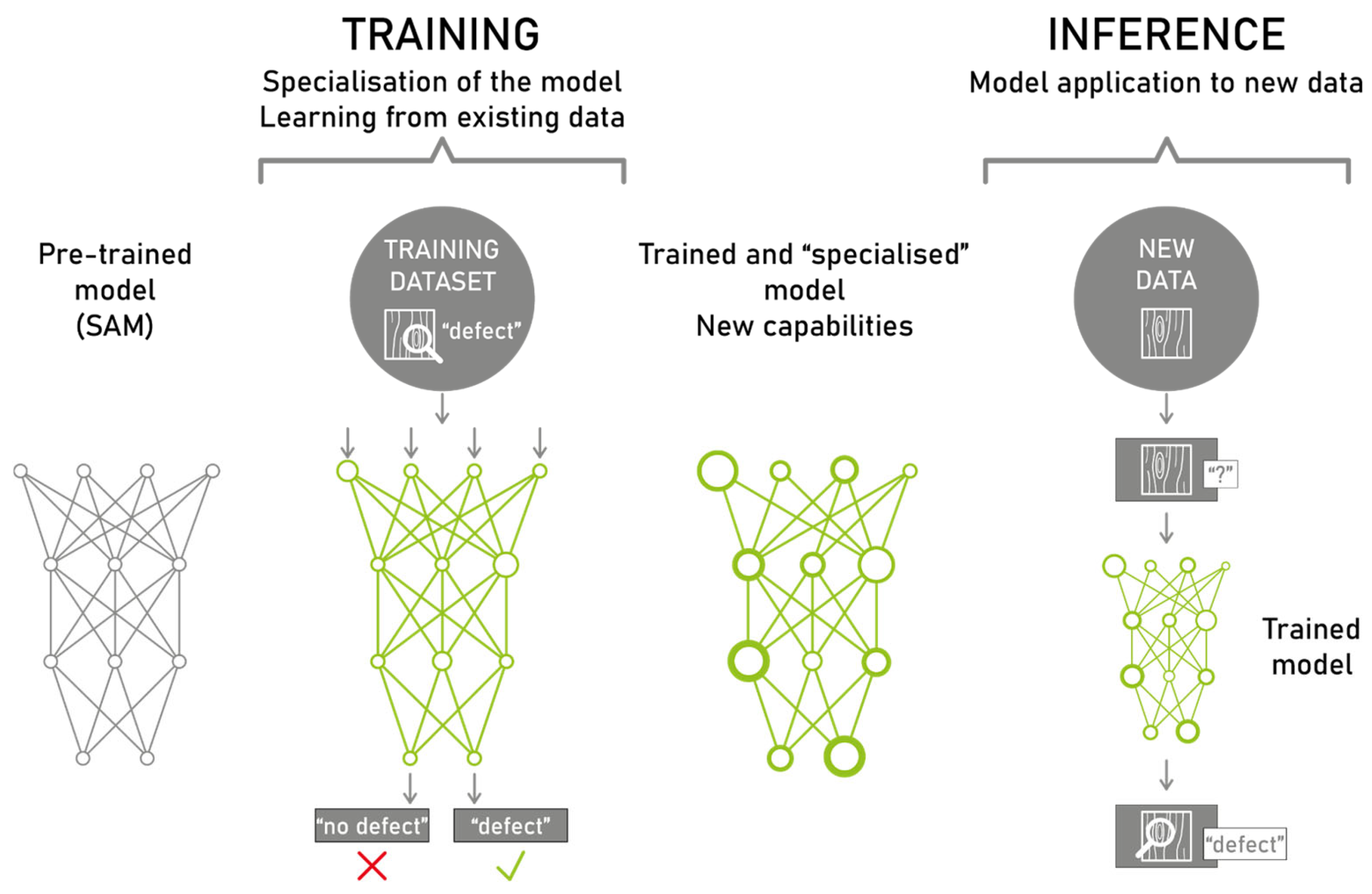
3.1.1. Introduction to SAM Fine-Tuning

The recognition of wood surface defects has been extensively investigated in academic research. Although existing methods have achieved high detection accuracy, they are consistently limited by the initial data acquisition phase, which is particularly time and resource intensive. Traditional approaches require the collection of thousands of annotated images and the generation of corresponding segmentation masks, often relying on extensive data augmentation to improve model performance—sometimes involving over 100,000 synthetic samples [30,31].

Given these constraints, particularly the cost and time associated with building large, high-quality datasets, this study explores the potential of recent image segmentation models capable of zero-shot generalization, which promise effective performance without task-specific retraining.

Among those currently available in the literature [32], the pre-trained Segment Anything Model (SAM), developed by Meta AI, was chosen for the study for image segmentation that can perform zero-shot generalization [33]: the dataset used for its training, i.e., SA-1B, the largest in existence, consisted of more than 11 million images and 1.1 billion masks.

Recent research has attempted to apply the Segment Anything Model (SAM), developed by Meta, to the task of wood surface defect segmentation. However, the results have been unsatisfactory, particularly when using the model’s Everything mode, which fails to accurately capture fine-grained defect boundaries in real-world industrial contexts [34]. These conclusions were further confirmed through direct testing of the publicly available SAM demo interface, which consistently showed poor segmentation performance on wood defect images. Despite its notable zero-shot performance, SAM exhibited limited accuracy in the segmentation of wood knots when using bounding box prompts. As demonstrated in the comparative segmentation results replicable using the official SAM online demo [35] and illustrated in Figure 6, the model consistently failed to delineate wood knots with sufficient precision. It frequently incorporated surrounding wood grain, cracks, and other unrelated textural elements, thereby compromising the specificity required for accurate defect identification.

To address these shortcomings, a fine-tuning phase was conducted. During this stage, the decoder parameters responsible for mask generation were updated using datasets focused on wood defects.

A key objective of the present research was to demonstrate the feasibility of fine-tuning a pre-trained computer vision model for accurate, task-specific segmentation using a limited dataset that a single annotator can independently produce.

3.1.2. Dataset Preparation for Fine-Tuning

The training datasets used in this study consisted of images of cut timber surfaces and their corresponding ground-truth masks—binary black-and-white images in which wood knots (considered as defects) are highlighted in white.

Four different datasets were employed during the fine-tuning phase to assess whether accurate segmentation of wood defects could be achieved without relying on large-scale datasets, which are often expensive and time-consuming to produce independently. The two base datasets were Dataset 1, a publicly available dataset [36] comprising 20,276 images of wooden planks with corresponding segmentation masks; and Dataset 2, a manually curated dataset, independently acquired and annotated by a single researcher, consisting of 60 images of glulam beams with corresponding ground-truth masks.

During the dataset preparation phase, several filtering and preprocessing steps were performed. For Dataset 1, all images with either empty masks or masks that did not contain wood knots (e.g., masks indicating only cracks, mold stains, or resin pockets) were excluded. This filtering step was not necessary for Dataset 2, as it had been created specifically for the project and already included only relevant masks.

Subsequently, the images and their corresponding masks from both Dataset 1 and Dataset 2 were divided into 256 × 256-pixel patches. Patches with empty corresponding masks were discarded from further use. This preprocessing step resulted in a total of 6760 patches (with masks) of 256 × 256 pixels derived from Dataset 1, and 642 patches (with masks) of the same size obtained from Dataset 2 (Figure 7).

To enhance generalization, we applied data augmentation to both datasets using fixed-angle transformations: (i) 90° rotation, (ii) horizontal and vertical flips, and (iii) random rotations within the range 2° ≤ x ≤ 40°. These augmentations were implemented using the torchvision.transforms.functional and torchvision.transforms.v2 modules from the PyTorch (version 2.4.0 + CUDA 12.1) framework [37].

The choice of rotations and flips was informed by established practices in the computer vision community, where such transformations have been shown to improve robustness without introducing noise—unlike in datasets where orientation carries categorical meaning [38].

Data augmentation techniques were then applied to Datasets 1 and 2. These included 90° rotations, mirroring, and random angle rotations; as a result of these augmentations, two additional datasets were generated, namely Dataset 3 and Dataset 4. Data augmentation was a necessary step to improve the generalization performance of the fine-tuned model. In the original datasets, the wood grain was consistently aligned vertically, introducing a strong directional bias. This could have led the model to overfit vertical grain patterns during training and perform poorly when encountering images with different grain orientations (e.g., horizontal or diagonal) during inference. The four datasets used in the fine-tuning phase were as follows:

Dataset 1: 6760 patches (256 × 256 pixels);

Dataset 2: 642 patches (256 × 256 pixels);

Dataset 3: 53,117 patches (256 × 256 pixels)—augmentation of Dataset 1;

Dataset 4: 5099 patches (256 × 256 pixels)—augmentation of Dataset 2.

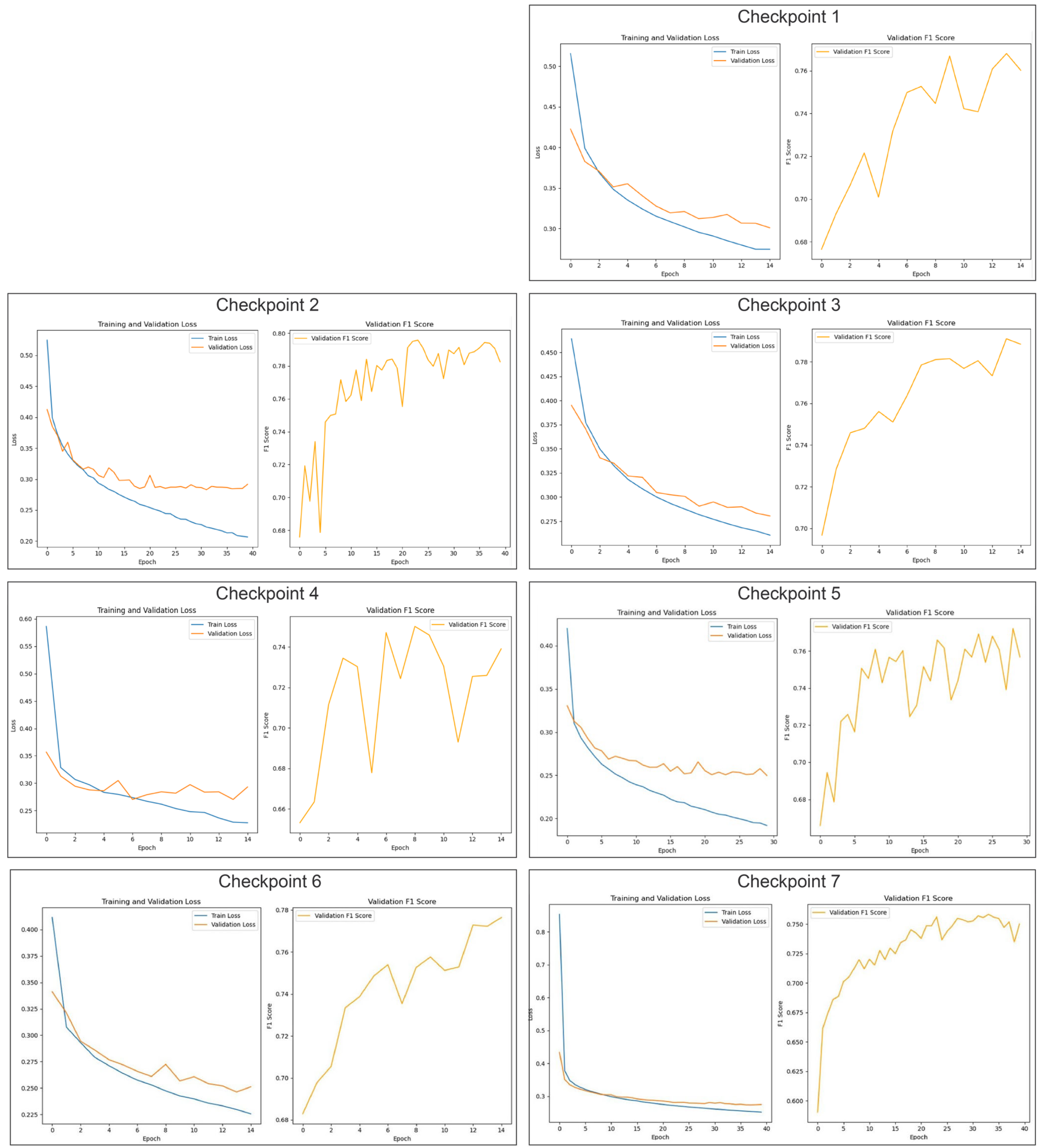
3.1.3. Fine-Tuning Process

The Segment Anything Model consists of three core components: a vision encoder, which extracts visual features from the input image; a prompt encoder, which encodes the input prompts (such as masks, bounding boxes, or points); and a mask decoder, which generates segmentation masks based on the encoded visual and prompt features. During fine-tuning, only the parameters of the mask decoder were updated, while those of the vision encoder and prompt encoder remained fixed. This approach preserved the feature extraction capabilities of the vision encoder, given its established generalization across a wide range of image-related tasks.

The Adam optimizer was employed to update the mask decoder weights [39]. Optimization was performed using a composite Dice Cross-Entropy (Dice CE) loss function, which integrates both region-based (Dice) and pixel-wise (Cross-Entropy) loss components [40].

During fine-tuning, three hyperparameters were varied: the number of epochs, the learning rate, and the weight decay. The specific values and tested combinations are summarized in

Table 1. Overview of the seven checkpoints produced during the training phase, along with their corresponding datasets. The first three checkpoints were trained on a public dataset, while the last four utilized an internally and autonomously generated dataset. The table reports the number of patches used for training each checkpoint and the three hyperparameters adjusted: epochs, weight decay, and learning rate. For the first three checkpoints, only the number of patches and epochs were varied, with weight decay and learning rate held constant. In the last four checkpoints, weight decay and learning rate were also adjusted in an effort to improve performance. Following this table, training loss and validation loss graphs are presented for each checkpoint to assess potential overfitting—clearly observed in checkpoints 2 and 5—alongside the validation F1 score graphs for all seven checkpoints.

Checkpoint	Dataset	Patches	Epochs	WeightDecay	LearningRate
Ch1	Dataset 1	6.760	15	0	1 × 10−5
Ch2	Dataset 1	6.760	40	0	1 × 10−5
Ch3	Dataset 3	53.117	15	0	1 × 10−5
Ch4	Dataset 2	642	15	0	1 × 10−5
Ch5	Dataset 4	5.099	30	0	1 × 10−5
Ch6	Dataset 4	5.099	15	1 × 10−4	1 × 10−5
Ch7	Dataset 4	5.099	40	1 × 10−4	1 × 10−6

. Each dataset was randomly split into training and validation subsets, with 80% of the data used for training and 20% for validation. This proportion was adopted as it is a standard practice in segmentation studies, although no formal cross-validation was applied. Model performance on the validation set was assessed using the F1 score [41]. The F1 score was computed exclusively for the positive class, corresponding to the white pixels representing wood defects, without averaging with the F1 score of the negative class (black pixels, i.e., background). This decision was motivated by the significant class imbalance in the binary masks, where the defect pixels were substantially underrepresented compared to the background. Averaging across both classes would have resulted in an artificial increase—approximately 15%—in the overall F1 score, thereby reducing its relevance to the primary objective of accurately assessing defect segmentation performance. Additionally, Dice CE loss was calculated during both training and validation to monitor potential overfitting. Training and validation curves showing the evolution of both metrics across epochs are provided in Table 1.

In cases where the validation loss diverged or increased while training loss decreased, changes in hyperparameters (e.g., adding a small weight decay or reducing the learning rate) were introduced to counter overfitting.

Results of the training phase consisted of seven checkpoints. Each checkpoint corresponds to the model state achieving the highest F1 score on the validation set at that time. No averaging was performed, and no single best checkpoint was preselected, since all were tested later on the independent inference datasets, as detailed in Section 3.1.5.

All trained model checkpoints and training scripts are publicly available in [42], ensuring reproducibility of the results.

3.1.4. Dataset Preparation for Inference

Although the F1 score was computed for each of the seven checkpoints during training, it is important to note that these evaluations were conducted on a validation set comprising 20% of the original dataset. As a result, there remained a substantial overlap in image characteristics, such as exposure, distortion, and resolution, between the training and validation sets, potentially biasing the evaluation. To more rigorously assess the generalization capability of the model checkpoints, two entirely new and independently acquired inference datasets, with distinct visual properties, were introduced to guide the final checkpoint selection (the detailed selection criteria are discussed in Section 3.1.5). As stated before in Section 2.2, all data acquisition procedures were carried out by a single operator using a different camera (industrial smart camera Keyence IV4-G500CA) than that employed during the training phase. The inference datasets consisted of raw images of wooden glulam beams, resulting in two distinct sets: the Far_100 dataset, comprising 65 images captured at a distance of 100 cm from the target surface, and the Near_70 dataset, consisting of 65 images acquired at a distance of 70 cm to provide larger visual representations of the defects [42]. Since the two inference datasets contained original and unlabeled images, ground-truth masks were manually created by the same operator using Adobe Illustrator 2024 (version 28.6) [43], by drawing white shapes over a black background to segment all visually identifiable wood defects. A consistent protocol was followed to ensure inter-image consistency, based on visual visibility, contour clarity, and the inclusion of all defect types relevant to the study, and to enable the future calculation of the F1 score metric (Figure 8).

Both datasets, along with the corresponding annotations, are publicly available as referenced in [42], to ensure full reproducibility.

3.1.5. Inference Pipeline Configuration

The segmentation performance of the fine-tuned model was evaluated by analyzing and comparing the behavior of the seven checkpoints across the two previously defined inference datasets. Each of the seven model variants was tested independently on both datasets, enabling the assessment of performance variation as a function of the distance between the imaging device and the wooden beam under inspection.

The seven checkpoints were evaluated during the inference phase on both test datasets, resulting in a total of 14 separate performance measurements, as illustrated in

Table 2. Comparison of the 14 iterations performed across the 7 checkpoints using the two inference datasets, Far_100 and Near_70. For testing, the three hyperparameters (adaptive threshold, minimum size, and patch size) were selected through an iterative process to maximize F1 score in segmentation performance.

Checkpoint	Inference_Dataset	adp_Threshold	min_Size	Patch_Size	Mean F1 Score	std_dev	std_Error	CI_95_Low	CI_95_High
Ch1	Far-100	0.8	30	256	0.353	0.167	0.021	0.312	0.394
Ch1	Near-70	0.12	30	512	0.315	0.223	0.028	0.259	0.370
Ch2	Far-100	0.8	30	256	0.274	0.173	0.021	0.231	0.317
Ch2	Near-70	0.5	30	512	0.269	0.247	0.031	0.208	0.330
Ch3	Far-100	0.8	30	256	0.178	0.154	0.019	0.140	0.217
Ch3	Near-70	0.5	30	512	0.225	0.215	0.027	0.171	0.278
Ch4	Far-100	0.12	10	256	0.659	0.110	0.014	0.631	0.686
Ch4	Near-70	0.12	10	512	0.657	0.175	0.022	0.613	0.700
Ch5	Far-100	0.4	10	256	0.600	0.141	0.017	0.566	0.635
Ch5	Near-70	0.12	10	512	0.681	0.167	0.021	0.639	0.722
Ch6	Far-100	0.8	0	256	0.563	0.157	0.020	0.524	0.602
Ch6	Near-70	0.12	10	512	0.628	0.200	0.025	0.579	0.678
Ch7	Far-100	0.4	10	256	0.608	0.150	0.019	0.571	0.645
Ch7	Near-70	0.12	10	512	0.686	0.150	0.019	0.649	0.723

. The F1 score was used as the primary metric for evaluation to choose the optimal checkpoint.

Preliminary tests revealed that the segmentation pipeline, in its default configuration, often failed to achieve optimal results. To address these limitations, an iterative parameter optimization procedure was implemented. This process targeted three key hyperparameters within the segmentation script: adaptive threshold, minimum size, and patch size. The adaptive threshold adjusts local thresholds to improve segmentation under varying lighting conditions. The minimum size filters out small noise or artifacts, improving accuracy without losing valid defects. A patch size of 512 × 512 pixels was selected for the Near_70 dataset, while a size of 256 × 256 pixels was adopted for Far_100. This choice was based on maintaining consistency between the knot-to-patch area ratio observed during training and that encountered during inference. When knots occupy disproportionately large regions within a patch, the model may fail to capture contextual boundaries, leading to inaccurate predictions.

It is essential to clarify that this procedure does not involve additional fine-tuning of the model weights. Instead, it represents an inference-level optimization in which segmentation parameters are adapted to the characteristics of real-world application data to enhance model output without retraining. All three parameters were systematically adjusted for each checkpoint, and the resulting masks were compared against the input images to evaluate segmentation accuracy. Table 2 describes the checkpoint parameters (adp_threshold, min_size, patch_size) with the best segmentation performances.

Among the checkpoints fine-tuned from the publicly available dataset, Checkpoint 1 exhibited the highest performance, achieving a mean F1 score of 0.353 with a standard error of ±0.021. In contrast, the best-performing model overall was Checkpoint 7, which had been fine-tuned on the custom dataset generated internally. This model achieved a mean F1 score of 0.686 (±0.019) (Figure 9) and was consequently selected for integration into the Woodot system for subsequent deployment. A side-by-side comparison between Checkpoint 1 and Checkpoint 7 is presented in Figure 10 and Figure 11.

3.2. The Five Woodot Subsystems

3.2.1. Rover Handling

In the first phase, for the rover to cruise the space, avoiding collisions, the work environment has to be pre-mapped to identify spatial constraints and include reference points for operations. The surroundings can also be explored on-the-fly, which is more practical in highly variable settings where the presence of obstacles may change frequently due to ongoing activities [18], but it was deemed unnecessary in this condition, with a predefined layout of the glulam beams and without any un-signaled workers crossing the scene.

Obstacle-avoidance and navigation on incoherent portions of the pavement are handled by generating dynamic point clouds to map the surroundings through the LiDAR sensor and complementing the virtual environment by employing stereo-camera vision sensors with 3D perception in order to detect objects, classify them, and determine their spatial position [18]. Once a work plan has been established, a vehicle’s mission can be defined in advance using ROS (Robot Operating System), setting common waypoints near each beam, and including navigation parameters like the appropriate speed, the waypoint trajectory interpolation, and the main vehicle’s orientation when approaching objects. Navigation is then managed by planning algorithms that use pre-collected data, a detailed work plan, and real-time obstacle detections to continuously control the vehicle’s movement, monitor its behavior, and correct any deviations from the expected path. RRT was used with an extend function for efficient and smooth mobile robot motion planning.

The first Docker service that was deployed is thus responsible for monitoring the state of the rover, continuously checking a digital input on the robot controller to begin communication with the robot arm.

When the rover is in a particular state, near the beam in correspondence to a predefined rover waypoint, this service opens a socket and streams a specific configuration to the robot arm. This configuration causes the end-effector of the robot arm to rotate, positioning the camera orthogonally to the selected portion of the beam surface (Figure 12).

3.2.2. Image Acquisition

The tests for the Woodot project were undertaken at the INDEXLAB laboratory in Lecco, Italy, and precisely in a covered outdoor area next to the parking, where the lighting conditions are characterized by uniform, low-intensity lighting, providing consistent but subdued illumination across the entire space. Since the light levels are kept low to minimize energy consumption while maintaining adequate visibility, the lighting is evenly distributed, ensuring there are no stark contrasts or shadows, and in no place are direct lights pointed at or near the testing area.

At a fixed working distance of 1000 mm from the target surface, the Canon EOS 1200D equipped with a standard EF-S 18–55 mm lens is capable of capturing a field of view corresponding to approximately 0.47 m².

Its higher resolution, broader coverage, and adjustable optics make it more suitable for this particular task, involving variable acquisition conditions (especially in terms of the quality of the indoor lighting) and the possibility to manually change the camera focus to overcome image-acquisition errors.

In fact, even if the dataset used for training the model had been created employing the Keyence IV4-G500CA smart camera, the lack of dynamic focusing capability, compounded by its significantly lower spatial resolution and narrower field of view, limits its effectiveness in applications requiring fine-grained visual detail and adaptable framing. Under identical distance conditions, the Keyence smart camera captures a significantly narrower field of view of 0.12 m², amounting to only 25% of the area covered by the Canon DSLR system.

This substantial difference is primarily attributed to the optical characteristics and sensor format of the two imaging systems. The Canon EOS 1200D, equipped with an APS-C CMOS sensor, offers considerable spatial detail, enabling flexible control over the image-acquisition process. Conversely, the Keyence IV4-G500CA utilizes a CMOS sensor measuring approximately 0.876 cm.

The second service, dedicated to camera streaming, employs the “gphoto2” [44] library to set up the Canon DSLR camera to acquire photos with selected shutter speed, aperture, and ISO settings. These images are then saved to a shared folder, accessible to the other services within the infrastructure.

The camera matrix for the DSLR is calculated using a calibration process on a chessboard, captured from various angles and distances. Key feature points in the chessboard corners are spotted to serve as the basis for establishing the link between the real-world coordinates of the pattern and their 2D representations on the image. With these data, a camera calibration algorithm is used to optimize the intrinsic parameters of the camera by minimizing the re-projection error. The output is the intrinsic camera matrix, a 3 × 3 matrix encoding information of the focal lengths in the x and y directions, which is used to undistort the captured images.

3.2.3. Image Elaboration for Defect Identification

As the image analysis module of Woodot is based on a deep learning pipeline (Figure 13) tailored for wood surface inspection employing SAM, the primary objective is the identification of knots through segmentation. This approach involves pixel-wise classification of images to distinguish defect regions from intact wood. As evaluated in the previous section, the F1 score achieved by checkpoint 7, equal to 0.69, demonstrated its superiority in the task of wood knot segmentation, thereby identifying it as the most suitable choice among the tested models.

The defect identification Docker service scans the shared folder for the captured photos and employs the model to detect and draw bounding boxes around any identified defects. The centroid coordinates of these bounding boxes are then saved to a text file on the shared folder for the subsequent operation to be performed. The conversion of segmentation outputs into bounding boxes [45,46,47,48,49,50] for defective localization tasks is often used in other industries and in the analysis of medical images.

The thresholding criteria that were used to exclude some knots over others were based on shape classification (one dimension of the bounding box could not exceed three times the other dimension) and constraints in size (the maximum diameter size of the knot could not exceed thirty millimeters), directly referring to the timber glulam beams that were used in the fair.

3.2.4. Defect Removal

Another Docker service is responsible for streaming the milling trajectories to the Doosan robot. Similar to the first service, it opens a socket and transmits the necessary trajectories to the robot, allowing it to perform the required milling operations (Figure 14).

Before streaming, a Python (version 3.11.9) script opens Grasshopper3D, and the real robot arm position and configuration are simulated. Every defect’s centroid corresponds to a certain wooden plug diameter coherent with the milling job settings. Within this simulation, the centroid coordinates from the segmentation process are ingested, and the script derives the necessary milling trajectories based on various parameters, such as the desired cutting speed, depth, and tool width. The depth of the cut was generally 12 mm, employing 6 passes at 35 mm/s with a spindle speed of roughly 18,000 RPMs, and always the same spindle, with a diameter of 8 mm.

The script generates a series of waypoints that the robot arm must follow to effectively mill the identified defects, while also ensuring that any potential collisions are avoided and singularities are circumvented. When planning the path, it was ensured that the robot operated within its allowable joint limits to prevent the encounter of limit configurations. Specifically, in order to avoid wrist singularities, the larger defect recognition and milling task was broken into smaller sub-tasks with intermediate waypoints to ensure the arm would not get too close to problematic configurations. By using joint-space path planning instead of Cartesian space path planning, “risky” configurations were limited to predefined configurations in correspondence to these waypoints. The adherence to the surface of the beam is ensured by the impedance control of the collaborative robot, which is very useful for any milling, polishing, or grinding tasks where the robot needs to maintain a consistent contact force.

To simulate the behavior of the Doosan robot within the Grasshopper3D environment, the script utilizes Visose’s “Robots” [51] plugin, which provides a custom interface for simulating programs with robotic systems.

Finally, a custom post-processor that was developed to translate geometric information from the Grasshopper3D simulation into the robot code required by the Doosan H2515 robot enables the trajectory-streamer service to send milling instructions to the physical robot arm.

3.2.5. Insertion of Restoration Material

The final task is to turn the end-effector and place the plug in correspondence to the milled hole (Figure 15), and finally to signal the rover that the job is finished and to move to the next waypoint.

Wooden plugs are grouped in batches on the collaborative robot’s end-effector, where a manual pre-check is conducted before the insertion to ensure proper placement and alignment. Once the plugs are in place, the robotic arm moves to an approach point in correspondence with the milled hole on the surface.

A spiral search routine is thus initiated, and the end-effector, rotated on the side of the plugs, wanders along a gradually widening spiral path (a motion function already built-in the Doosan control library), a method designed to locate the hole with precision.

As the arm searches the hole, its built-in collision control mechanism continuously monitors for any signs of contact. When the plug impacts the intended target, identified by a change in force feedback from the collision sensor, the system recognizes that the correct hole has been found. At that moment, the robot transitions from its search behavior to an insertion action, aligning itself accurately with the milled hole.

During insertion, the plug is gently pushed into the opening, with the collision control ensuring that the interaction is safe and that no excessive force is applied to either the plug or the surrounding structures. Once the insertion is complete, the arm moves in the Z direction and turns back to its home position on the rover, outputting a signal to go on to the next portion of the beam.

4. Results

The performance of the Woodot system was evaluated by testing its complete autonomous workflow on real curved laminated timber beams in a laboratory environment at INDEXLAB, Lecco and in the context of the SAIE Fair in Bologna on 9 October 2024. The results are presented according to the system’s key functional modules: navigation and positioning, defect identification accuracy, and repair operation.

4.1. Navigation and Positioning Performance

Woodot’s rover demonstrated reliable autonomous navigation in unstructured environments, including cluttered workshop floors and variable lighting conditions. The integrated LiDAR sensors enabled safe maneuvering and obstacle avoidance. The robot consistently achieved positional tolerances within ±1 cm relative to the target beam location. Switching between global navigation and local alignment mode allowed the robot to precisely position the arm within the operational workspace of the beam, adapting to different geometries and beam curvatures.

4.2. Defect Identification Accuracy

Regarding the fine-tuning of the SAM segmentation model, the checkpoints derived from the autonomously generated dataset (Checkpoints 4–7) consistently outperformed those obtained from the public dataset (Checkpoints 1–3). Despite being ten times smaller in size, the autonomous dataset yielded checkpoints with a mean F1 score of 0.635, representing a 2.3× improvement over the public dataset checkpoints, which achieved a mean F1 score of 0.269. In addition to superior segmentation performance, fine-tuning on the autonomous dataset required approximately 40% less computational time and resources.

These F1 score metrics are reported as the mean of checkpoints 1–2–3 (public dataset) and separately as the mean of checkpoints 4–5–6–7 (autonomous dataset). While the limited sample size does not support formal statistical testing, the observed performance trends are consistent and meaningful within the experimental setup. This suggests that, for the specific task of wood defect segmentation, compact and task-oriented datasets can be effectively used to fine-tune generalist models like SAM. Nevertheless, caution should be exercised when extrapolating this finding to other domains: the observed efficiency gains and performance improvements may depend heavily on the characteristics of the task and the visual domain involved. Therefore, the reduction in dataset size should be considered a promising direction.

This study highlights the potential for developing and publishing lightweight, autonomous “micro-datasets”, thus broadening the applicability of segmentation models to image domains underrepresented in existing large-scale datasets.

The system successfully detected knots of varying size, shape, and wood grain contrast, with a false positive rate under 12% and a false negative rate under 15% in optimal lighting conditions. Defect localization precision was measured as the Euclidean distance between ground truth and predicted mask centroids, averaging 4.3 mm. These percentages are derived from qualitative assessments performed on a small set of representative samples.

4.3. Restoration Workflow Effectiveness

It is important to note that a manual insertion check was always performed in advance to be sure the tolerances for the plug insertion were met before the actual robotic movement. The physical process of plug insertion was tested and validated under controlled conditions in INDEXLAB’s laboratory environment during this iteration of the system; following these experiments, the trials indicated high mechanical repeatability. While none of the tests were repeated under very different working conditions (e.g., different types of wood, surface roughness, wood moisture level, and lighting conditions) within roughly 25 evaluated insertions performed, the robotic arm followed pre-planned milling trajectories with a dimensional tolerance of ±0.5 mm in diameter and ±0.2 mm in depth. Plug insertion was tested on cylindrical wood inserts with three different sizes, and the success rate of flush placement without visual gaps (inspected through direct visual inspection) was 87% in the first pass. The search time was around 16 s for each plug. The remaining cases were due to minor misalignment in tool calibration, which will be addressed in the next development phase.

4.4. Operational Cycle Time

A full knot repair cycle (detection, classification, milling, and plug insertion) took an average of 74 s per defect, including all inter-module communication and repositioning time, with a clear bottleneck on the detection portion of the process, taking about 35% of the total operational cycle time. The benchmarking was conducted on a total batch of 25 milling operations, with 10% of outliers—corresponding to instances of poor recognition—excluded from the analysis. Compared to traditional manual operations (due to limited formal data availability, some metrics were informally estimated using sector-specific knowledge and sources from the wood industry), which typically range from 3 to 5 min per knot depending on beam complexity, Woodot’s process offers a time reduction of over 60%, with a significant improvement in repeatability and reduced operator fatigue.

These results validate the effectiveness of Woodot as a mobile robotic system for autonomous visual quality control and aesthetic restoration of curved laminated beams. Further refinements in calibration, tool handling, and model robustness are expected to enhance performance in real production environments.

5. Discussion

The implementation and testing of the Woodot system reveal both the opportunities and the challenges associated with deploying intelligent mobile robotics in the domain of curved glulam beam processing.

The system presented in the context of the paper was implemented using hardware that is approximately 10 years old. Limitations and bottlenecks concerning the performance of this hardware setup are clearly stated. However, this also highlights a promising aspect of the research: the system functions well even under constrained hardware conditions. Future developments will certainly consider updated hardware platforms, which are expected to further improve its performance and efficiency.

Compared to static robotic cells or CNC-based defect handling, Woodot’s mobility enables it to service non-standard and geometrically complex timber components without predefined positioning, making it uniquely suited for dynamic workshop conditions, as shown in the video [52]. The deployment of AI-driven segmentation significantly enhances defect detection accuracy and adaptiveness, as demonstrated by the quantitative performance of the trained SAM-based model. In particular, the use of a small but application-specific dataset yielded higher F1 scores than larger generic datasets, reinforcing the value of tailored data in industrial AI applications.

From an operational standpoint, Woodot demonstrated significant time efficiency compared to manual repair of knots, offering consistent results with lower physical and cognitive workload for human workers. Nonetheless, the current limitations in human–machine collaboration, particularly in the context of collaborative robotics, highlight the need for enhanced skills in these augmented manufacturing jobs.

Simple block-programming or visual scripting features, teaching via manual hand-guiding with rewards and penalties, and interaction with the robot software with advanced typing features, are all features used to effectively engage the operator in the use of this robotic system—to gamify the experience with the machine. To improve this collaboration, it is essential to develop more user-friendly applications that can be directly accessed on the robot’s Teach Pendant. These applications should facilitate manual guidance of the robot, allowing operators to visualize actions through intuitive graphical user interfaces (GUIs). Additionally, integrating augmented reality (AR) visors can provide operators with a real-time view of the robot’s environment, enhancing their understanding and interaction with the robotic system even more.

While these are still bottlenecks of the Woodot application in this early stage of development, if addressed carefully, they will grant wide operability in real-world production environments. By addressing these areas, we can foster a more seamless and productive partnership between humans and robots in various industrial applications.

Future development will focus on improving tool-changer reliability, expanding the plug insertion toolkit, and planning further fine-tuning on additional datasets, including other timber species and engineered wood products such as CLT, to improve segmentation robustness across diverse surface textures and finishes. Additionally, the efficient containerization using Docker enables a more optimal use of resources in the future. By packaging applications and dependencies, Docker allows for seamless deployment to any cloud-based infrastructure, with the possibility of using an orchestration platform like Kubernetes to manage and scale containers as needed across a cluster of machines, ensuring high availability, scalability, and efficiency.

We plan to validate the cloud-based architecture by measuring system latency and scalability under varying loads, testing fault tolerance through simulated failures, and monitoring resource usage and uptime of Docker/Kubernetes services.

By setting up a “Rhino.Compute” [53] service to call a cloud-based server, it would be possible to offload computationally intensive tasks to the cloud, thereby enhancing processing efficiency and reducing the local workload on the host machine. Multiple requests can be called concurrently, deploying Rhino.Compute in a production environment, such as a Windows-based VM or a headless server, monitoring the performance and optimizing it as needed to ensure efficient use of resources and minimize cycle time and computational costs. Rhino.Compute performance will also be evaluated under real-time task conditions.

These developments will significantly reduce the load of computing image segmentation and robot path-planning on the host machine.

6. Conclusions

Woodot introduces a novel paradigm in timber defect repair, effectively bridging adaptive robotics with the practical constraints of workshop-level production. Its architecture and results provide a foundation for further research and industrial application in wood construction automation. From a technological perspective, Woodot combines mobility, perception, and manipulation into a unified platform capable of autonomously identifying and repairing wood knot defects. This integration allows for intervention in environments where traditional linear automation systems are ineffective or impractical.

While the mechanical performance of the milling and plugging modules still requires fine-tuning for full automation, the current system already enables a semi-autonomous workflow with clear productivity and quality advantages. Nevertheless, some limitations remain. These include the dependency on stable lighting conditions for optimal vision performance and the need for tool calibration checks.

References

1. Amiri, A.; Ottelin, J.; Sorvari, J.; Junnila, S. Cities as Carbon Sinks—Classification of Wooden Buildings. Environ. Res. Lett. 2020, 15, 094076. [Google Scholar] [CrossRef]
2. Dzhurko, D.; Haacke, B.; Haberbosch, A.; Köhne, L.; König, N.; Lode, F.; Marx, A.; Mühlnickel, L.; Neunzig, N.; Niemann, A.; et al. Future Buildings as Carbon Sinks: Comparative Analysis of Timber-Based Building Typologies Regarding Their Carbon Emissions and Storage. Front. Built Environ. 2024, 10, 1330105. [Google Scholar] [CrossRef]
3. APA—The Engineered Wood Association. Technical Note: Glulam Appearance Classifications for Construction Applications; APA: Tacoma, WA, USA, 2010; Available online: https://www.apawood.org/publication-search?q=y+110&tid=1 (accessed on 28 May 2025).
4. APA—The Engineered Wood Association. ANSI 117-2020: Standard Specification for Structural Glued Laminated Timber of Softwood Species; APA: Tacoma, WA, USA, 2020; Available online: https://www.apawood.org/publication-search?q=ansi+117&tid=1 (accessed on 28 May 2025).
5. Rothoblaas Srl. TAPS—Timber Caps. Available online: https://www.rothoblaas.com/products/tools-and-machines/wood-repair-items/taps (accessed on 28 May 2025).
6. Hirsch, R.; Hahn, C.; Jäger, W. Nachweis Der Feuerwiderstandsklasse von Mauerwerk—Aktuelle Aussagen Im Rahmen Der Überarbeitung von DIN 4102:1994-03 Und DIN 4102-4/A1:2004-11 Sowie DIN 4102-22:2004-11. Mauerwerk 2009, 13, 203–206. [Google Scholar] [CrossRef]
7. Hashim, U.R.; Hashim, S.Z.M.; Muda, A. Automated vision inspection of timber surface defect: A review. J. Teknol. 2015, 77, 1–10. [Google Scholar] [CrossRef]
8. Biederman, M. Robotic Machining Fundamentals for Casting Defect Removal. Master’s Thesis, Oregon State University, Corvallis, OR, USA, 2016. [Google Scholar]
9. Li, R.; Zhong, S.; Yang, X. Wood Panel Defect Detection Based on Improved YOLOv8n. BioResources 2025, 20, 2556–2573. [Google Scholar] [CrossRef]
10. Andersson, P. Automated Surface Inspection of Cross Laminated Timber. Master’s Thesis, University West, Trollhättan, Sweden, 2020. [Google Scholar]
11. Nagata, F.; Kusumoto, Y.; Fujimoto, Y.; Watanabe, K. Robotic sanding system for new designed furniture with free-formed surface. Robotics Comput. Integr. Manuf. 2007, 23, 371–379. [Google Scholar] [CrossRef]
12. Timber Products Company. Robots Introduced to Grants Pass—Automated Panel Repair Line. Available online: https://timberproducts.com/robots-introduced-to-grants-pass/ (accessed on 19 April 2025).
13. Toman, R.; Rogala, T.; Synaszko, P.; Katunin, A. Robotized Mobile Platform for Non-Destructive Inspection of Aircraft Structures. Appl. Sci. 2024, 14, 10148. [Google Scholar] [CrossRef]
14. Giftthaler, M.; Sandy, T.; Dörfler, K.; Brooks, I.; Buckingham, M.; Rey, G.; Kohler, M.; Gramazio, F.; Buchli, J. Mobile Robotic Fabrication at 1:1 Scale: The In Situ Fabricator. Constr. Robot. 2017, 1, 3–14. [Google Scholar] [CrossRef]
15. Huo, Y.; Chen, D.; Li, X.; Li, P.; Liu, Y.-H. Development of an Autonomous Sanding Robot with Structured-Light Technology. arXiv 2019, arXiv:1903.03318. [Google Scholar] [CrossRef]
16. Rossini, L.; Romiti, E.; Laurenzi, A.; Ruscelli, F.; Ruzzon, M.; Covizzi, L.; Baccelliere, L.; Carrozzo, S.; Terzer, M.; Magri, M.; et al. CONCERT: A Modular Reconfigurable Robot for Construction. arXiv 2025, arXiv:2504.04998. [Google Scholar] [CrossRef]
17. Sigma Ingegneria. Il Sistema Woodot per l’edilizia del futuro: Un rover con Braccio Robotico per le Travi Lamellari. Blog Sigma—SAIE 2024 Preview, 26 September 2024. [Google Scholar]
18. Ruttico, P.; Pacini, M.; Beltracchi, C. BRIX: An autonomous system for brick wall construction. Constr. Robot. 2024, 8, 10. [Google Scholar] [CrossRef]
19. FBR Ltd. Hadrian X®|Outdoor Construction & Bricklaying Robot from FBR. Available online: https://www.fbr.com.au/view/hadrian-x (accessed on 29 May 2025).
20. Helm, V.; Ercan, S.; Gramazio, F.; Kohler, M.; Willmann, J.; Dörfler, K.; Giftthaler, M.; Buchli, J.; Sandy, T.; Rey, G.; et al. Mobile Robotic Fabrication on Construction Sites: DimRob. In Proceedings of the 2012 IEEE/RSJ International Conference on Intelligent Robots and Systems (IROS), Vilamoura, Portugal, 7–12 October 2012; IEEE: Piscataway, NJ, USA, 2012; pp. 2684–2689. [Google Scholar] [CrossRef]
21. Helm, V.; Willmann, J.; Gramazio, F.; Kohler, M. In-Situ Robotic Fabrication: Advanced Digital Manufacturing Beyond the Laboratory. In Gearing up and Accelerating Cross-Fertilization Between Academic and Industrial Robotics Research in Europe: Technology Transfer Experiments from the ECHORD Project; Röhrbein, F., Veiga, G., Natale, C., Eds.; Springer Tracts in Advanced Robotics; Springer: Cham, Switzerland, 2014; Volume 94, pp. 63–83. [Google Scholar] [CrossRef]
22. Patil, S.; Vasu, V.; Srinadh, K.V.S. Advances and perspectives in collaborative robotics: A review of key technologies and emerging trends. Discov. Mech. Eng. 2023, 2, 13. [Google Scholar] [CrossRef]
23. Faccio, M.; Granata, I.; Menini, A.; Milanese, M.; Rossato, C.; Bottin, M.; Minto, R.; Pluchino, P.; Gamberini, L.; Boschetti, G.; et al. Human factors in cobot era: A review of modern production systems features. J. Intell. Manuf. 2023, 34, 85–106. [Google Scholar] [CrossRef]
24. Fang, X.; Luo, Q.; Zhou, B.; Li, C.; Tian, L. Research Progress of Automated Visual Surface Defect Detection for Industrial Metal Planar Materials. Sensors 2020, 20, 5136. [Google Scholar] [CrossRef]
25. Reu, P.; Sweatt, W.; Miller, T.; Fleming, D. Camera System Resolution and Its Influence on Digital Image Correlation. Exp. Mech. 2014, 55, 9–25. [Google Scholar] [CrossRef]
26. Arza-García, M.; Núñez-Temes, C.; Lorenzana, J.A.; Gutiérrez, J.J. Evaluation of a Low-Cost Approach to 2-D Digital Image Correlation vs. a Commercial Stereo-DIC System in Brazilian Testing of Soil Specimens. Arch. Civ. Mech. Eng. 2022, 22, 4. [Google Scholar] [CrossRef]
27. Available online: https://www.dewalt.co.uk/product/d26200-gb/8mm-14-fixed-base-router (accessed on 20 August 2024).
28. KEYENCE. IV4-500CA Vision Sensor. KEYENCE America. Available online: https://www.keyence.com/products/vision/vision-sensor/iv4/models/iv4-500ca/ (accessed on 28 May 2025).
29. Robert McNeel & Associates. Grasshopper3D. Available online: https://www.grasshopper3d.com/ (accessed on 20 August 2024).
30. He, T.; Liu, Y.; Xu, C.; Zhou, X.; Hu, Z.; Fan, J. A Fully Convolutional Neural Network for Wood Defect Location and Identification. IEEE Access 2019, 7, 123453–123462. [Google Scholar] [CrossRef]
31. Yang, Y.; Wang, H.; Jiang, D.; Hu, Z. Surface Detection of Solid Wood Defects Based on SSD Improved with ResNet. Forests 2021, 12, 1419. [Google Scholar] [CrossRef]
32. Zou, X.; Yang, J.; Zhang, H.; Li, F.; Li, L.; Wang, J.; Wang, L.; Gao, J.; Lee, Y.J. Segment Everything Everywhere All at Once. arXiv 2023, arXiv:2304.06718. Available online: https://arxiv.org/abs/2304.06718 (accessed on 29 May 2025).
33. Meta AI. Segment Anything GitHub Repository. Available online: https://github.com/facebookresearch/segment-anything (accessed on 20 August 2024).
34. Ji, W.; Li, J.; Bi, Q.; Liu, T.; Li, W.; Cheng, L. Segment Anything Is Not Always Perfect: An Investigation of SAM on Different Real-world Applications. Mach. Intell. Res. 2024, 21, 617–630. [Google Scholar] [CrossRef]
35. Meta AI. Introducing Segment Anything: Working Toward the First Foundation Model for Image Segmentation. Meta AI Blog, 2023. Available online: https://ai.meta.com/blog/segment-anything-foundation-model-image-segmentation/ (accessed on 29 May 2025).
36. Kodytek, P.; Bodzas, A.; Bilik, P. A large-scale image dataset of wood surface defects for automated vision-based quality control processes. F1000Research 2022, 10, 581. [Google Scholar] [CrossRef] [PubMed]
37. TorchVision Contributors. TorchVision: Image Transformations for PyTorch. 2023. Available online: https://pytorch.org/vision/stable/index.html (accessed on 29 May 2025).
38. Kumar, T.; Mileo, A.; Brennan, R.; Bendechache, M. Image Data Augmentation Approaches: A Comprehensive Survey and Future Directions. arXiv 2023, arXiv:2301.02830. Available online: https://arxiv.org/abs/2301.02830 (accessed on 26 May 2025). [CrossRef]
39. PyTorch Contributors. torch.optim.Adam—PyTorch Documentation. Available online: https://docs.pytorch.org/docs/stable/optim.html#torch.optim.Adam (accessed on 27 May 2025).
40. MONAI Consortium. monai.losses.DiceCELoss—MONAI Documentation. Available online: https://docs.monai.io/en/stable/losses.html#monai.losses.DiceCELoss (accessed on 27 May 2025).
41. Scikit-Learn Developers. sklearn.metrics.f1_score—scikit-learn Documentation. Available online: https://scikit-learn.org/stable/modules/generated/sklearn.metrics.f1_score.html (accessed on 27 May 2025).
42. Deval, M.; Bianchi, F.; Moroni, C. Wood knots defects dataset [Data set]. Zenodo 2025. [Google Scholar] [CrossRef]
43. Adobe Inc. Adobe Illustrator (Version 2024) [Software]. Available online: https://www.adobe.com/products/illustrator.html (accessed on 27 May 2025).
44. gphoto.org. gPhoto Website. Available online: http://gphoto.org/ (accessed on 20 August 2024).
45. Weimer, D.; Scholz, P.; Klein, L.; Merhof, D. Segmentation-Based Deep-Learning Approach for Surface-Defect Detection. arXiv 2019, arXiv:1903.08536. Available online: https://arxiv.org/abs/1903.08536 (accessed on 29 May 2025).
46. Ye, Y.; Huang, Q.; Liu, Y.; Fan, X.; Lu, S. Reference-Based Defect Detection Network. arXiv 2021, arXiv:2108.04456. Available online: https://arxiv.org/abs/2108.04456 (accessed on 29 May 2025).
47. Nair, A.; Asari, V.K. Detection and Segmentation of Manufacturing Defects Using Deep Convolutional Neural Networks and Transfer Learning. Sensors 2019, 19, 4262. [Google Scholar] [CrossRef]
48. Ibarra-Castanedo, C.; Gonzalez, D.; Maldague, X. Automatic Defects Segmentation and Identification by Deep Learning Algorithm with Pulsed Thermography. J. Imaging 2019, 5, 9. [Google Scholar] [CrossRef]
49. Chen, Y.; Wu, T.; Yeh, C.; Lin, B. YOLOSeg with Applications to Wafer Die Particle Defect Segmentation. Micromachines 2024, 15, 378. [Google Scholar] [CrossRef]
50. Zhao, Y.; Liu, Y.; Wang, L.; Liu, S.; Zhang, S. The Amalgamation of Object Detection and Semantic Segmentation for Steel Surface Defect Detection. Appl. Sci. 2022, 12, 6004. [Google Scholar] [CrossRef]
51. Visose. Robots GitHub Repository. Available online: https://github.com/visose/Robots (accessed on 20 August 2024).
52. IndexLab. Woodot. Available online: https://www.indexlab.it/woodot (accessed on 20 August 2024).
53. Robert McNeel & Associates. Rhino3D Compute Developer Guide. Available online: https://developer.rhino3d.com/guides/compute/ (accessed on 20 August 2024).
Figure 1. Traditional manual defect removal process in glulam beams, as currently practiced in industrial wood lamination production. The images illustrate the high physical demand due to the operators’ working posture, as well as the significant mental effort required to maintain prolonged concentration for accurate detection and removal of knots. Additionally, continuous manual control of the router’s rotation adds to operator fatigue and task complexity.
Sustainability 17 05574 g001
Figure 2. The Woodot system displayed at the SAIE Fair in Bologna on 9 October 2024.
Sustainability 17 05574 g002
Figure 3. The five key subsystems of Woodot.
Sustainability 17 05574 g003
Figure 4. The three main components of Woodot: the rover, the robot, and the end-effector.
Sustainability 17 05574 g004
Figure 5. The different end-effector configurations integrate camera, router, and wood plugs in an aluminum carter.
Sustainability 17 05574 g005
Figure 6. From the left: original image; mask prediction with the “everything” function; mask prediction with bounding box corresponding to the size of the image; mask prediction with bounding box corresponding to a specific wood knot.
Sustainability 17 05574 g006
Figure 7. From the left: Dataset 1 patch; Dataset 1 patch mask; Dataset 2 patch; Dataset 2 patch mask.
Sustainability 17 05574 g007
Figure 8. From the left: Far_100 image; Far_100 mask; Near_70 image; Near_70 mask.
Sustainability 17 05574 g008
Figure 9. Mean F1 score of the 7 checkpoints based on the two inference datasets (Far_100, Near_70). A clear performance gap in terms of F1 score is observed between checkpoints trained on the public dataset (Checkpoints 1–3) and those trained on the in-house dataset (Checkpoints 4–7), with the latter achieving approximately double the performance. Except for Checkpoint 1, all models consistently perform better on closer-range images (Near_70 dataset).
Sustainability 17 05574 g009
Figure 10. Comparison between the best-performing checkpoint obtained from the public dataset (Checkpoint 1) and the one trained on the internally produced dataset (Checkpoint 7), based on the F1 score. From left to right: original image; ground truth mask; mask prediction produced by Checkpoint 1 evaluated on inference dataset Far_100 (F1 score = 0.353); and mask prediction produced by Checkpoint 7 evaluated on inference dataset Far_100 (F1 score = 0.608). Checkpoint 1 exhibits several false positives, indicating low segmentation reliability.
Sustainability 17 05574 g010
Figure 11. Comparison between the best-performing checkpoint obtained from the public dataset (Checkpoint 1) and the one trained on the internally produced dataset (Checkpoint 7), based on the F1 score. From left to right: original image; ground truth mask; mask prediction produced by Checkpoint 1 evaluated on inference dataset Near_70 (F1 score = 0.315); and mask prediction produced by Checkpoint 7 evaluated on inference dataset Near_70 (F1 score = 0.686). Checkpoint 7 clearly outperforms Checkpoint 1 in defect segmentation, as the latter misinterprets the wood’s glare as a defect.
Sustainability 17 05574 g011
Figure 12. Close-up of the end-effector rotation to perform camera acquisition.
Sustainability 17 05574 g012
Figure 13. Fine-tuning workflow of SAM, highlighting three key stages: (i) the pre-training phase, where the model learns general features from a large and diverse dataset; (ii) the fine-tuning phase, where the model is adapted to specific datasets to improve performance for wood defect detection; (iii) the inference phase, during which the trained model applies the learned knowledge to new, unseen data to generate segmentations without further parameter updates.
Sustainability 17 05574 g013
Figure 14. Close-up of the end-effector while milling the wood knot on the timber beam surface. The precision of the toolpath as it adapted to the irregular grain and hardness of the knot area was within a tolerance of about ±0.5 mm in diameter and ±0.2 mm in depth.
Sustainability 17 05574 g014
Figure 15. Close-up of the restored surface of the wooden glulam beam. The flush insertion of the plug was achieved using a spiral toolpath trajectory motion of the Doosan arm to center the milled hole.
Sustainability 17 05574 g015