Robust Optimization of Multimodal Transportation Route Selection Based on Multiple Uncertainties from the Perspective of Sustainable Transportation

Abstract

Multimodal transportation is of strategic significance in improving transportation efficiency, reducing costs and achieving low-carbon development, all of which contribute to sustainable transportation. However, in actual operation, it often encounters multiple uncertain challenges such as demand, transportation time and carbon trading price, making it difficult for traditional fixed-parameter route optimization to meet the requirements of complex situations. Based on robust optimization and Box uncertainty set, this paper constructs a hybrid robust stochastic optimization model of multimodal transportation routes with uncertain demand, transportation time and carbon trading price, designs a hybrid algorithm, and verifies the effectiveness and rationality of the model through a numerical example. The results indicate that different types of uncertainty influence the routing decisions through distinct mechanisms. That is, demand uncertainty mainly affects capacity allocation and cost structure, transportation time uncertainty increases time penalties, and carbon trading price uncertainty drives preference for low-emission modes. Compared with the single genetic algorithm and the simulated annealing algorithm, the hybrid algorithm has better performance in terms of cost and stability. The hybrid robust stochastic optimization model can handle the multimodal transportation route selection problems where the probability distribution of parameters is unknown well. It is beneficial for decision-makers to adjust the uncertain budget level according to their preferences to formulate scientific transportation plans, so as to achieve sustainable transportation development.

1. Introduction

Each mode of transportation has its advantages. Railway transportation is a very cost-effective mode of transportation, and air transportation is the fastest way of cargo transportation [1]. Multimodal transportation, as an efficient and intensive transportation mode, has attracted much attention in recent years driven by market demand due to its significant advantages in reducing carbon emissions, optimizing transportation cost and improving resource utilization efficiency [2]. However, it is highly complex, involving the connection and coordination of multiple transportation modes, the balance of interests among different participants, as well as wide temporal and spatial coverage, making it extremely vulnerable to interference from internal and external factors. The interfering factors bring significant uncertainties, making the system parameters fluctuate and the probability distribution difficult to predict accurately [3]. These uncertainties directly affect the stability of multimodal transportation systems, leading to increased transportation costs, higher risks of delays, and difficulties in unifying economic benefits with environmental goals.

In the actual transportation process, there are different types of uncertainties. The frequent fluctuations in the demand for goods make it difficult for enterprises to precisely allocate transportation capacity, resulting in the idleness of some resources or insufficient transportation capacity, thereby bringing greater challenges to route planning and dispatching arrangements. As customers’ personalized demands for delivery time continue to rise, this not only requires more flexible transportation routes but also more efficient scheduling strategies. However, transportation time and transfer efficiency are often affected by external factors such as weather and traffic, and the changes are difficult to predict, resulting in high-cost risks for multimodal transportation operators when formulating and implementing transportation plans. The fluctuations in carbon trading price not only increase the uncertainty of operating costs but also make it more difficult to achieve a balance between economic benefits and environmental goals [4].

To assist multimodal transportation operators in designing transportation plans that are economical, robust and environmentally friendly, this paper considers three uncertain factors, namely demand, transportation time and carbon trading price, and explores the robust optimization of multimodal transportation routes to help enterprises achieve sustainable development in the complex and changeable transportation environment. Based on the induction and summary of existing research, this paper will construct a hybrid robust stochastic optimization model for multimodal transportation routes, design the solution algorithm, and conduct case analysis, with the aim of providing decision-making references for sustainable transportation under multi-factor interference.

2. Literature Review

In recent years, multimodal transportation has received extensive attention, especially the issue of its route optimization, which has become a key research topic. Some studies have mainly explored multimodal transportation route selection under certain conditions [5,6,7,8]. However, due to the constraints of practical conditions, researchers have turned to route optimization strategies under uncertainties to cope with dynamic transportation demands and achieve environmental goals.

Regarding the uncertainties, the existing research has mainly focused on demand and transportation time. Li and Sun [9], Peng [10] and Liu et al. [11] discussed the selection of multimodal transportation routes under the condition of uncertain demand. Peng et al. [12], Wang et al. [13] and Guo et al. [14] explored the influence of uncertain transportation time on the selection of multimodal transportation routes. Zhang et al. [15] and Li et al. [16] studied the optimization of multimodal transportation routes under the dual uncertainties of demand and transportation time. With the development of the green concept, researchers have begun to analyze the impact of fluctuations in carbon trading prices on the selection of multimodal transportation routes. Peng et al. [17] indicated through random scenario analysis that the fluctuation of carbon trading price prompts enterprises to give priority to low-carbon transportation methods. Li et al. [18] balanced the cost and environmental benefits under the uncertainty of carbon emissions through fuzzy nonlinear programming.

In terms of the goal setting for multimodal transportation route selection, minimizing the comprehensive cost has been the most common goal. Transportation costs have generally been taken into account. In addition, transshipment costs, time penalty costs and carbon emission costs are also be considered. Hou et al. [19] and Sun [20] established a multimodal transportation route optimization model that minimizes the total cost, including transportation cost and carbon emission cost. Xu et al. [21] and Han et al. [22] comprehensively considered the transportation cost and transshipment cost. Zhu [23] and Zhang et al. [24] further incorporated the comprehensive impact of time cost and environmental cost. Gao et al. [25] analyzed the route optimization of multimodal transportation under the carbon tax policy. Reşat and Türkay [26] explored the costs and environmental impacts of the design of multimodal transportation networks.

For various uncertain factors, different methods have been applied to solve the route selection of multimodal transportation, mainly including the interval number method, scenario analysis method, stochastic programming and robust optimization. The interval number rule limited the fluctuation range of uncertain parameters by upper and lower bounds [12]. The scenario analysis method simulated parameter changes by constructing multiple possible scenarios [13]. If more accurate probability distribution information can be obtained, the stochastic programming method can be used, which is modeled based on the known probability distribution [10]. When it is difficult to determine the exact distribution, robust optimization could ensure that the decision still has good performance in the worst case, especially with the assistance of methods such as Box uncertain sets, triangular fuzzy numbers [18,20,22] and trapezoidal fuzzy numbers [16,24].

Overall, there have been relatively abundant research achievements on the selection of multimodal transportation routes under uncertain conditions. The main research situations are shown in

Table 1. Comparison of existing studies on multimodal transportation route selection.

Category	Uncertainty			Objective Function				Model
Factor	Demand	Transportation Time	Carbon Trading Price	Transportation Cost	Transshipment Cost	Time Penalty Cost	Carbon Emission Cost	Robust Optimization
Reference
Li and Sun (2022) [9]	✓		✓	✓	✓	✓	✓	✓
Peng (2024) [10]	✓							Mixed Integer Programming
Liu et al. (2025) [11]	✓			✓	✓			✓
Peng et al. (2021) [12]		✓		✓	✓	✓		✓
Wang et al. (2024) [13]		✓		✓	✓			Integer Programming
Guo et al. (2024) [14]		✓						Mixed Integer Programming
Zhang et al. (2021) [15]	✓	✓		✓	✓	✓	✓	✓
Li et al. (2023) [16]	✓			✓			✓	Fuzzy Optimization
Peng et al. (2024) [17]	✓		✓	✓	✓			✓
Li et al. (2024) [18]				✓	✓	✓	✓	Fuzzy Optimization
Hou et al. (2024) [19]	✓	✓		✓		✓	✓	✓
Sun (2020) [20]		✓		✓	✓	✓	✓	Fuzzy Optimization
Xu et al. (2024) [21]		✓		✓	✓			✓
Han et al. (2023) [22]	✓			✓	✓			Fuzzy Optimization
Zhu (2022) [23]		✓						Mixed Integer Programming
Zhang et al. (2024) [24]	✓			✓	✓		✓	Fuzzy Optimization
Gao et al. (2024) [25]				✓			✓	Integer Programming
Reşat and Türkay (2015) [26]		✓		✓				Mixed Integer Programming

Note: A “✓” indicates that this factor was taken into account in the relevant literature.

. The existing studies have mainly considered the uncertain factors of demand, time and carbon trading price, but there were relatively few studies that took all three factors into account simultaneously. Transportation costs have been basically taken into account in the optimization objectives, but studies that have considered multiple costs simultaneously are not very sufficient. Meanwhile, existing research showed that robust optimization models could effectively assist in analyzing the route selection of multimodal transportation under uncertainty.

In view of this, this paper intends to study the robust optimization of multimodal transportation route selection under multiple uncertainties. Different from previous studies, this research has the following main characteristics:

(1)

We take into account three uncertain factors, namely demand, transportation time and carbon trading price, simultaneously.

(2)

The decision-making objective is used to minimize the total cost including transportation cost, transshipment cost, time penalty cost and carbon emission cost.

(3)

We construct a multimodal transportation route optimization model based on hybrid robust stochastic optimization.

3. Model Construction

3.1. Problem Description

In a multimodal transportation system, enterprises need to transport goods from the origin to the destination through various modes of transportation such as highway, railway and waterway, and pass through several transfer nodes during the process, as shown in Figure 1. The selection of transportation routes needs to be balanced among multiple transportation modes, as there are significant differences among different modes in terms of transportation costs, transportation time and carbon emissions.

The selection of multimodal transportation routes is influenced by many uncertain factors. This study explores the impacts caused by the uncertainties of demand, time and carbon trading price. Demand uncertainty is manifested as the volatility and unpredictability of the demand for goods within different transportation cycles. Due to the influence of market changes, seasonal factors and customer preferences, etc., it is difficult for the allocation of transportation capacity and route planning to precisely match the actual demand. The uncertainty of transportation time stems from transportation delays and fluctuations in transfer efficiency caused by factors such as weather, traffic conditions, and equipment malfunctions, which directly affect the reliability of on-time delivery of goods and the feasibility of the route plan. The uncertainty of carbon trading price is driven by policy adjustments, market supply and demand relationships, and changes in the macroeconomic environment. Its fluctuations increase the complexity when considering the cost of carbon emissions, thereby affecting the balance between economic benefits and environmental goals of multimodal transportation. This study explores the comprehensive influence of triple uncertainties on the selection of multimodal transportation routes.

3.2. Symbol Explanation

In this study, the parameters involved and their corresponding meanings are shown in

Table 2. Definition and description of model parameters.

Category	Symbol	Implication
Set/Indices	$s$	Scenario index.
	$i,j$	Node indices.
	$k$	Transportation mode index.
	$l$	Transshipment mode index.
Parameters	$D$	Demand quantity.
	$d_{ij}^k$	Distance from node $i$ to node $j$, using transportation mode $k$.
	$c_k$	Unit transportation cost of using transportation mode $k$.
	$L_{kl}$	Transshipment cost at node from mode $k$ to mode $l$.
	${\tau }_i$	Processing time at node $i$.
	$T_{\min }$	Lower bound of the flexible time window.
	$T_{\mathrm{soft}}$	Range of the flexible time window.
	$p$	Time penalty cost coefficient.
	$e_k$	Carbon emissions of transportation mode $k$.
	$\alpha$	Carbon trading price.
	$a_D$	Average demand.
	${\delta }_D$	Uncertainty coefficient of demand.
	$a_{\alpha }$	Average carbon trading price.
	${\delta }_{\alpha }$	Uncertainty coefficient of carbon trading price.
	${\delta }_t\left(i,j,k\right)$	Uncertainty coefficient of transportation time.
Decision Variables	$x_{ijk}$	Decision variable of transportation route from node $i$ to node $j$ using mode $k$.
Auxiliary Variables	$u_D\left(s\right)$	Random variable of demand.
	$u_t\left(i,j\right)$	Uncertainty variable of transportation time.
	$u_{\alpha }\left(s\right)$	Random variable of carbon trading price.
	${\mathrm{\Gamma }}_D$	Demand uncertainty budget.
	${\mathrm{\Gamma }}_t$	Transportation time uncertainty budget.
	${\mathrm{\Gamma }}_{\alpha }$	Carbon trading price uncertainty budget.
	$S$	Set of all uncertainty scenarios.
	$P_s$	Probability of scenario $s$ occurring.

.

3.3. Model Assumptions

(1)

During transportation, the goods must remain as a whole and cannot be split or transported in batches.

(2)

Suppose that each transfer node and the available transportation mode all have sufficient processing and transportation capacity, and the supply constraints caused by insufficient capacity are not considered.

(3)

At the node, the goods are allowed to change the mode of transportation at most once, thereby reducing the additional costs and complexities caused by excessive transshipment.

(4)

This study focuses on multimodal transportation routes and transportation processes, without considering the site selection, construction or operation costs of warehousing facilities. It is assumed that all the transfer nodes have the necessary loading, unloading and turnover conditions.

(5)

Considering the complexity of the model, serious delays or force majeure factors caused by external emergencies such as weather, equipment failure or goods damage during transportation are not taken into account. However, by setting uncertainty sets or scenario sets for the fluctuations of key parameters such as demand, transportation time, and carbon trading price, the influence of random disturbances in reality can be reflected to a certain extent.

(6)

Goods have a certain sensitivity to transportation time, so a minimum time limit $T_{\min }$ and a soft time limit $T_{\mathrm{soft}}$ are set. When the total transportation time exceeds $T_{\min }$, the corresponding time penalty cost will be incurred. If the delay continues to exceed $T_{\min }+T_{\mathrm{soft}}$, the penalty cost will increase further.

(7)

The demand for goods will fluctuate, and the extent of the fluctuation is limited by the uncertain budget ${\mathsf{\Gamma }}_D$. The transportation time may vary within a certain range due to reasons such as traffic conditions and scheduling, and is controlled by the uncertain budget ${\mathsf{\Gamma }}_t$. Fluctuations in carbon trading price caused by changes in the market or policies are restricted by ${\mathrm{\Gamma }}_{\alpha }$.

(8)

Suppose the carbon emission factor (the emission coefficient per unit distance) is closely related to the specific mode of transportation, but for the same mode of transportation, this factor is fixed at the same distance. The cost of carbon emissions is also affected by the carbon trading price, represented by $\left(a_{\alpha }+{\delta }_{\alpha }\cdot u_{\alpha }\left(s\right)\right)$, and is constrained by the uncertainty budget ${\mathrm{\Gamma }}_{\alpha }$.

(9)

Suppose the occurrence probability $p_s$ of all scenarios $s\in S$ is known and satisfies ${\sum }_{s\in S}{p}_s=1$. In a multiple uncertain environment, various fluctuation situations in actual operation are characterized by applying the Box uncertain set and its corresponding budget ${\mathsf{\Gamma }}_D$, ${\mathsf{\Gamma }}_t$, and ${\mathrm{\Gamma }}_{\alpha }$ to the uncertain parameter $\{u_D(s),u_t(i,j),u_{\alpha }(s)\}$.

3.4. Model Formulation

3.4.1. Objective Analysis

The objective of multimodal transportation route selection considering multiple uncertainties is to minimize the comprehensive cost, specifically including transportation cost, transshipment cost, time penalty cost and carbon emission cost. It is elaborated, respectively, as follows.

(1) Transportation cost. Transportation cost refers to the expense incurred by choosing different transportation modes between nodes. The calculation of transportation cost is regarded as the sum of the products of unit freight rate, distance and uncertainty adjustment term when mode $k$ is selected between node $i$ and node $j$. $c_k$ represents the unit freight rate of mode $k$, $d_{ij}^k$ represents the distance from node $i$ to node $j$ adopting mode $k$, $\left(a_D+{\delta }_D\cdot u_D\left(s\right)\right)$ represents the deviation of the unit transportation cost under scenario $s$, and $\left(1+{\delta }_t\left(i,j,k\right)\cdot u_t\left(i,j\right)\right)$ represents the correction of the transportation time fluctuation to the cost. The transportation cost is expressed as:

$$C_1={\displaystyle \sum _{i=1}^n{\displaystyle \sum _{j=1}^n{\displaystyle \sum _{k=1}^3\left(a_D+{\delta }_D\cdot u_D\left(s\right)\right)}}}\times c_k\times d_{ij}^k\times x_{ijk}\times \left(1+{\delta }_t\left(i,j,k\right)\cdot u_t\left(i,j\right)\right)$$

(1)

(2) Transshipment cost. Transshipment cost refers to the expense incurred by the conversion of transportation mode. If mode $k$ is switched to mode $l$ at node $j$, transshipment cost will be incurred. Let $L_{kl}$ represent the transshipment cost from mode $k$ to mode $l$, considering the influences of $\left(a_D+{\delta }_D\cdot u_D\left(s\right)\right)$ and $\left(1+{\delta }_t\left(i,j,k\right)u_t\left(i,j\right)\right)$, the transshipment cost is expressed as:

$$C_2={\displaystyle \sum _{i=1}^{n-1}{\displaystyle \sum _{j=i+1}^n{\displaystyle \sum _{k=1}^3{\displaystyle \sum _{l=1}^3\left(a_D+{\delta }_D\cdot u_D\left(s\right)\right)}}}}\times L_{kl}\times x_{ijk}\times x_{j\left(i+1\right)l}\times \left(1+{\delta }_t\left(i,j,k\right)\cdot u_t\left(i,j\right)\right)$$

(2)

(3) Time penalty cost. To limit the timeout degree of the total transportation time, the minimum time limit $T_{\min }$ and the soft time limit $T_{\mathrm{soft}}$ are introduced, and the timeout part is described by ${\left(\cdot \right)}_{+}=\max \{\cdot ,0\}$. When ${\displaystyle \sum _{i=1}^n{\tau }_i}$ exceeds $T_{\min }$, a basic penalty will be imposed. If it continues to exceed $T_{\min }+T_{\mathrm{soft}}$, a higher penalty will be imposed. The time penalty cost is expressed as:

$$C_3=p\times {\left({\displaystyle \sum _{i=1}^n{\tau }_i}-T_{\min }\right)}_{+}+p\times {\left({\displaystyle \sum _{i=1}^n{\tau }_i}-\left(T_{\min }+T_{\mathrm{soft}}\right)\right)}_{+}$$

(3)

(4) Carbon emission cost. Carbon emission cost refers to the environmental cost brought about by carbon emissions during transportation, which is calculated based on the carbon emission factors, distance, and carbon trading price of each mode of transportation. Let the carbon emission factor of mode $k$ be $e_k$, the carbon emission price be expressed as $\left(a_{\alpha }+{\delta }_{\alpha }\cdot u_{\alpha }\left(s\right)\right)$ in scenario $s$, and the carbon emission cost can be expressed as:

$$C_4={\displaystyle \sum _{i=1}^n{\displaystyle \sum _{j=1}^n{\displaystyle \sum _{k=1}^3\left(a_D+{\delta }_D\cdot u_D\left(s\right)\right)}}}\times e_k\times d_{ij}^k\times x_{ijk}\times \left(a_{\alpha }+{\delta }_{\alpha }\cdot u_{\alpha }\left(s\right)\right)$$

(4)

3.4.2. Analysis of Model Constraints

To ensure the feasibility and scientific validity of the transportation decision-making model, in combination with the operational characteristics and actual demands of the multimodal transportation system, the following constraints are specially considered:

(1)

In the transportation network, the transportation of goods from any node to its next node is only allowed to adopt a single mode. This constraint is intended to simplify mode selection, reduce operational complexity, and enhance the controllability of the transportation process.

(2)

For each node in the network, the total input of goods must be equal to the total output. This constraint ensures that there is no unexplained increase or decrease in goods at the nodes, maintaining the consistency and integrity of the flow in the transportation system.

(3)

The disturbance of uncertain parameters during the transportation process needs to be limited by the budget parameters ${\mathrm{\Gamma }}_D$, ${\mathrm{\Gamma }}_t$ and ${\mathrm{\Gamma }}_{\alpha }$. By setting corresponding constraint conditions in the model and controlling the fluctuation amplitude of parameters, extreme deviations of the model solution caused by excessive perturbation can be avoided.

(4)

The total time of the entire transportation process shall not be lower than a reasonable minimum value. This constraint is set based on actual operational needs to ensure that the transportation timeliness meets the basic requirements while avoiding potential risks caused by excessively short durations.

(5)

The model characterizes the randomness of external disturbances through scenario probability and uncertainty budgeting. In multi-scenario analysis, the sum of the occurrence probabilities of each scenario $s$ must be equal to 1. This constraint follows the basic principles of probability theory to ensure the completeness and consistency of the scenario set.

3.4.3. Hybrid Robust–Stochastic Optimization Model for Multimodal Transportation Route Under Multiple Uncertainties

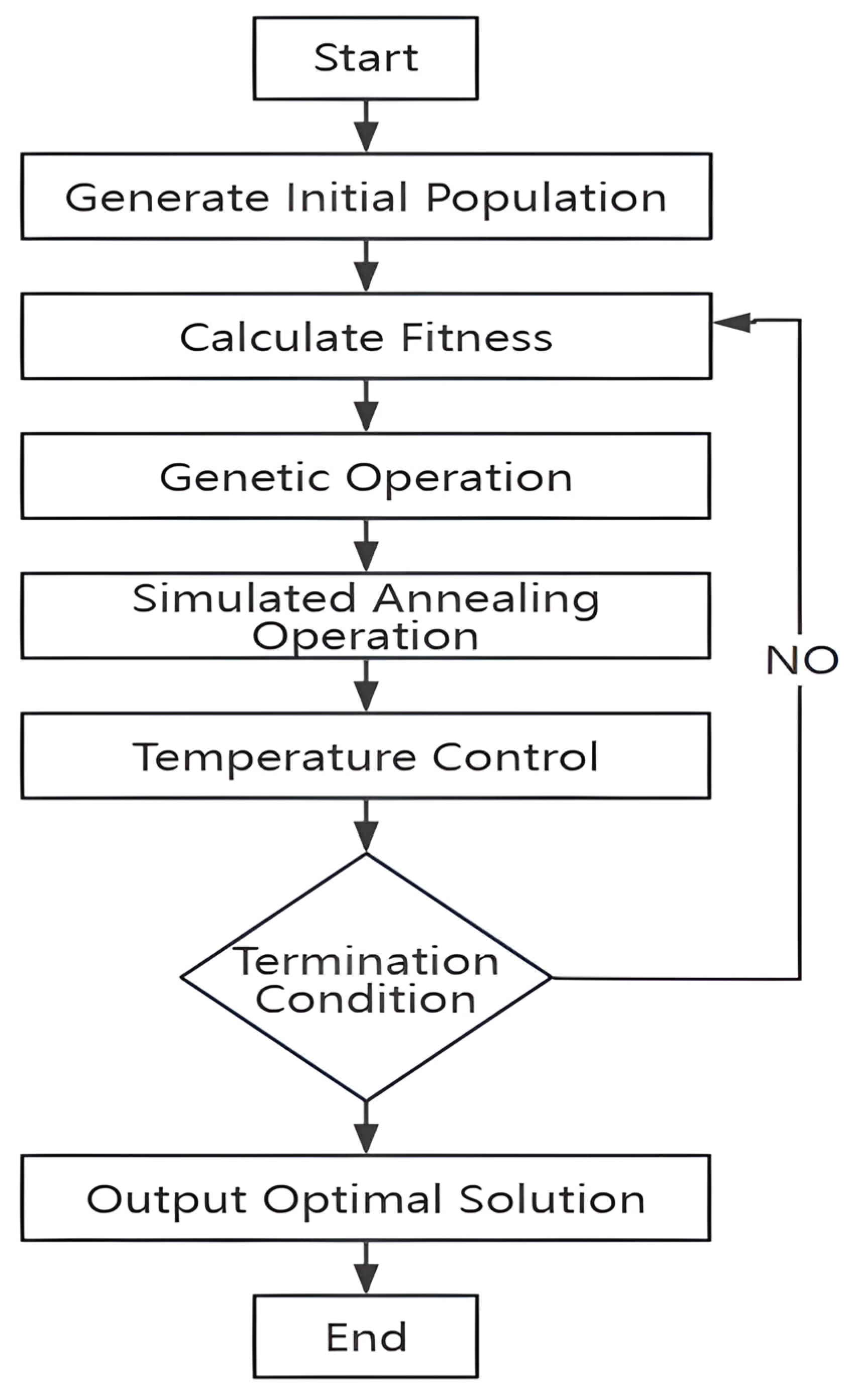
Based on the previous analysis, the objective function is the sum of transportation cost, transshipment cost, time penalty cost and carbon emission cost. The calculation formula is as follows:

$$\min C_{\mathrm{total}}={\displaystyle \sum _{s\in S}{p}_s}(C_1+C_2+C_3+C_4)$$

(5)

The model includes the following constraints:

$${\displaystyle \sum _{k=1}^3{\displaystyle \sum _{j=1}^n{x}_{ijk}}}=1,\forall i\in \{1,2,\dots ,n\}$$

(6)

$${\displaystyle \sum _{k=1}^3{\displaystyle \sum _{j=1}^n{x}_{ijk}}}={\displaystyle \sum _{k=1}^3{\displaystyle \sum _{l=1}^n{x}_{jil}}},\forall i\in \{1,2,\dots ,n\}$$

(7)

$${\displaystyle \sum _{i, j}{u}_t\left(i,j\right)}\le {\mathrm{\Gamma }}_t,{\mathrm{\Gamma }}_t\ge 1$$

(8)

$$\left|u_{\alpha }\right|\le {\mathrm{\Gamma }}_{\alpha },{\mathrm{\Gamma }}_{\alpha }\ge 1$$

(9)

$$u_D\le {\mathrm{\Gamma }}_D,{\mathrm{\Gamma }}_{\mathrm{D}}\ge 1$$

(10)

$$T_{\min }\le {\displaystyle \sum _{i=1}^n{\tau }_i}$$

(11)

$$x_{ijk}\in \{0,1\}$$

(12)

$${\displaystyle \sum _{s\in S}{p}_s}=1$$

(13)

Equation (5) indicates that the decision-making objective is to minimize the total cost in various scenarios. Each scenario $s\in S$ represents a joint realization of all three uncertain parameters, including demand, transportation time, and carbon trading price. A sample average approximation method is used to transform the continuous problem into a scenario-based form. Equation (6) is used to limit that only one mode of transportation can be selected between transportation nodes $i$ and $j$. Equation (7) stipulates that only one transfer operation can be carried out at node $i$. Equation (8) represents the uncertain budget constraint of transportation time. Equation (9) represents the uncertainty budget constraint of carbon trading price. Equation (10) represents the uncertain budget constraint of demand. Equation (11) indicates that when a node changes its transportation mode, it needs to match the transportation modes before and after. Equation (12) limits the specific value of the decision variable to 0 or 1. Equation (13) stipulates that the sum of the probabilities of occurrence of each scenario $s$ is 1.

4. Algorithm Design

Under the influence of multiple uncertainties such as demand, transportation time and carbon trading price, the multimodal transportation route optimization problem shows high complexity and nonlinearity, and often has the NP-hard characteristic [27]. To obtain better solutions and robustness in an uncertain environment, genetic algorithm (GA) and simulated annealing (SA) are widely applied. GA achieves global search through population evolution, while SA excels in local search and escaping from local optima. Existing studies have verified the advantages of the genetic-simulated annealing hybrid algorithm. Literature [28,29,30] indicated that the genetic-simulated annealing hybrid algorithm could improve the convergence speed, solution accuracy and robustness, providing effective support for this problem.

This study adopts the genetic-simulated annealing hybrid algorithm to optimize the multimodal transportation route selection. GA uses selection, crossover and mutation operations to search for global solutions, while SA accepts inferior solutions through the “cooling” strategy to enhance local search. To integrate the advantages of both, the algorithm is designed as follows: (1) Using dual coding of routes and transportation modes to generate the initial population, reflecting the diversity of multimodal transportation. (2) Construct the fitness function, comprehensively considering the uncertainties of demand, transportation time and carbon trading price. (3) Introduce the SA operation to enhance the local search ability. (4) Optimize crossover and mutation operations to enhance the overall effect. This algorithm can efficiently search for the global optimal solution under multiple uncertainties while avoiding local optima and improving the convergence speed and the quality of the solution. Its process is shown in Figure 2.

Step 1: Generate the initial population. Each individual represents a multimodal transportation route scheme and is represented by genetic coding. The specific encoding method is as follows: Each individual is composed of a series of genes, and each gene contains a node index and a transportation mode index. The node index represents the nodes in the multimodal transportation network, and the transportation mode index represents the transportation mode between nodes. The structural example of each individual is [origin, transportation mode, destination]. The origin and destination are represented by node indexes, which start from 0 and indicate different geographical locations. The mode of transportation is represented by integer values. For example, 1 represents highway, 2 represents railway, and 3 represents waterway.

Step 2: Calculate the fitness of each individual. The fitness function comprehensively considers transportation cost, transshipment cost, time penalty cost and carbon emission cost. The impact of fluctuations in demand, transportation time and carbon trading price on costs is characterized by introducing a set of Box uncertainty parameters. Transportation cost is calculated based on the mode of transportation and distance for each section of the journey and varies due to the uncertainty of demand. The transshipment cost is determined based on the transfer operation time and cost of the node, and the operation time is affected by the uncertainty of the transportation time. The time penalty cost is calculated when the arrival time of the goods exceeds the preset time window and varies due to the uncertainty of transportation time. Carbon emission cost is evaluated based on the carbon emission factor and distance for each transportation mode, and adjusted by carbon trading price uncertainty.

Step 3: Genetic Operation. Through the roulette selection mechanism, the selection probability is calculated based on each individual’s fitness, and high-quality individuals are selected to enter the next generation. During the crossover operation, two parent individuals are randomly selected, and a new offspring is generated through the crossover process. The intersection points are randomly selected. Then, mutation operations are performed on the offspring individuals, randomly changing the transportation mode or route to introduce new solutions to increase diversity. For example, in the route [1, 2, 2, 4, 1], randomly select the third gene and change its transportation mode from 2 (railway) to 1 (highway) to generate a new route [1, 2, 1, 2, 4, 1].

Step 4: Simulated annealing operation. For each individual, the neighborhood solution is generated by exchanging the positions of two nodes in the route or changing the transportation mode. For example, swap nodes 2 and 3 in the route [1, 2, 3, 2, 4, 1] to generate the neighborhood solution [1, 3, 2, 2, 4, 1]. If the fitness of the newly generated neighborhood solution is better than that of the current solution, the solution is directly accepted. Otherwise, calculate the acceptance probability according to the formula of simulated annealing. If a random number is less than this probability, the inferior solution is accepted. The acceptance probability formula is:

$$p(\mathrm{accept})=\exp \left({\displaystyle \frac{\mathrm{\Delta }f}{T}}\right)$$

(14)

where $\mathrm{\Delta }f$ represents the change in fitness, and $T$ denotes the current temperature.

Step 5: Temperature control. As the number of iterations increases, the temperature is gradually reduced to control the probability of accepting inferior solutions, with $T_0$ as the initial temperature. A linear cooling method is adopted, with the formula expressed as:

$$T=T_0\times (1-{\displaystyle \frac{Numberofiterations}{Maximumnumberofiterations}})$$

(15)

Step 6: Termination condition. The algorithm terminates when the number of iterations reaches a predetermined upper limit or when the quality of the solution meets the expected standard.

By using the above steps and combining genetic algorithm and simulated annealing, it is possible to better search for high-quality solutions in multimodal transportation scenarios, and by means of random perturbation to avoid falling into local extremum, thereby improving the overall convergence speed and solution quality.

5. Example Analysis

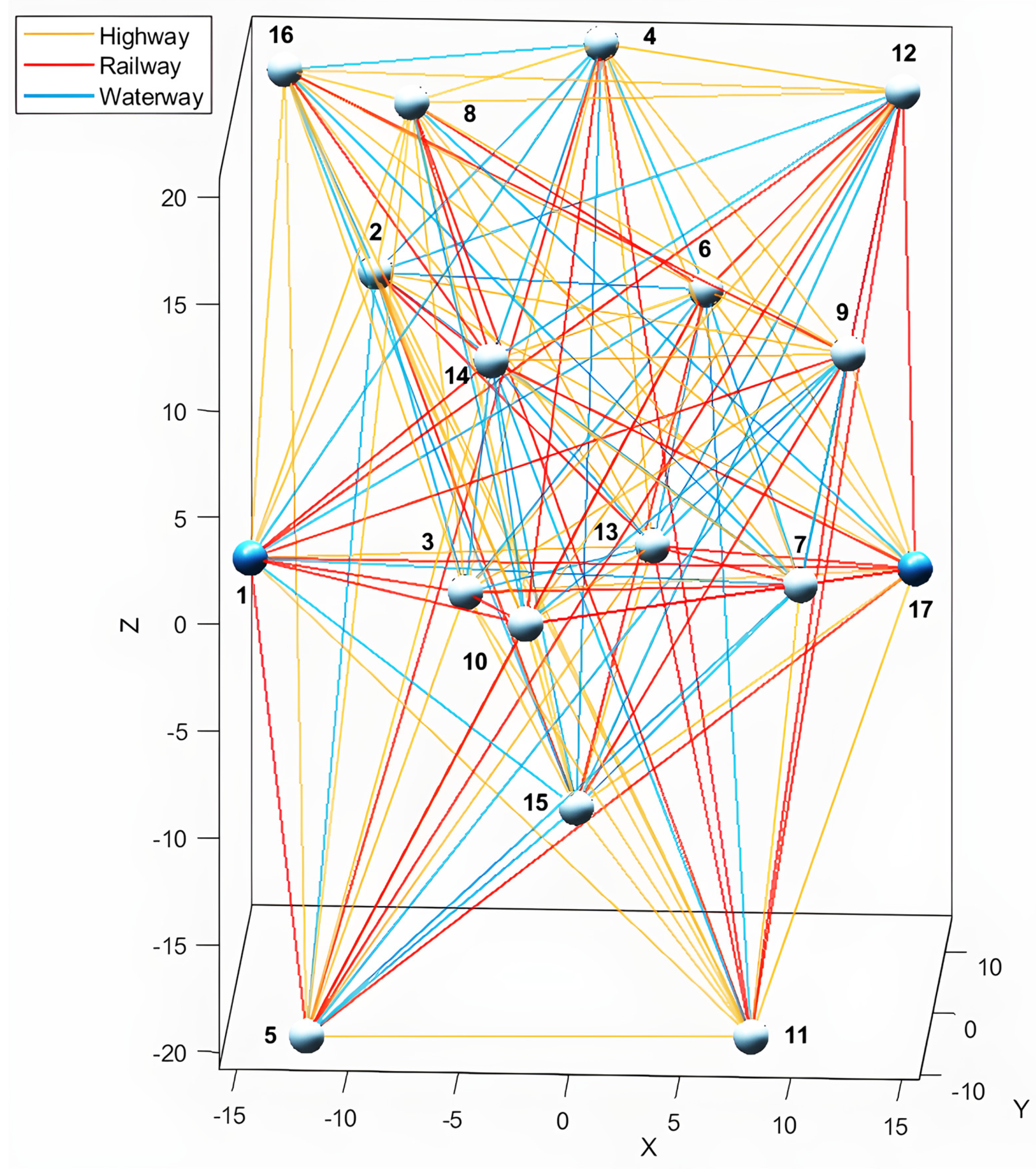
5.1. Case Information

There is a multimodal transportation system of highway, railway, waterway, involving 17 nodes, which are numbered from 1 to 17. Among them, node 1 and node 17 represent the origin and destination of transportation, respectively, as shown in Figure 3. The distances between each node are shown in the Appendix A

Table A1. Distance information between 17 nodes in the multimodal transportation system for case study. (Unit: km).

Node i	Node j	Highway Distance	Railway Distance	Waterway Distance	Node i	Node j	Highway Distance	Railway Distance	Waterway Distance
1	1	0	0	0	9	1	1700	1900	10,000
1	2	1200	1463	1600	9	2	1600	1800	1900
1	3	2100	2294	2300	9	3	1000	1200	1300
1	4	2200	2372	2400	9	4	1100	1300	1400
1	5	1100	1300	1400	9	5	1400	1600	1700
1	6	1000	1162	1300	9	6	1300	1500	1600
1	7	1050	1150	1300	9	7	700	800	900
1	8	1600	1800	10,000	9	8	800	1000	1100
1	9	1700	1900	10,000	9	9	0	0	0
1	10	1050	1200	10,000	9	10	600	700	800
1	11	650	700	10,000	9	11	900	1000	10,000
1	12	600	660	700	9	12	1600	1800	1900
1	13	850	900	1000	9	13	1900	2100	2200
1	14	1800	2050	2100	9	14	1700	1900	2000
1	15	1700	1900	2000	9	15	1400	1600	1700
1	16	1300	1500	10,000	9	16	1500	1700	1800
1	17	2300	2600	10,000	9	17	800	900	1000
2	1	1200	1463	1600	10	1	1050	1200	10,000
2	2	0	0	0	10	2	1300	1500	10,000
2	3	1300	1400	1500	10	3	1900	2100	10,000
2	4	1500	1600	1700	10	4	2000	2200	10,000
2	5	150	180	200	10	5	1100	1300	10,000
2	6	250	300	350	10	6	1000	1200	10,000
2	7	750	800	900	10	7	900	1000	10,000
2	8	1800	2000	10,000	10	8	700	800	900
2	9	1600	1800	1900	10	9	600	700	800
2	10	1300	1500	10,000	10	10	0	0	0
2	11	900	1000	1100	10	11	400	500	10,000
2	12	600	700	800	10	12	900	1000	10,000
2	13	900	1000	1100	10	13	1200	1300	1400
2	14	800	900	1000	10	14	1300	1500	1600
2	15	500	600	700	10	15	1000	1200	1300
2	16	700	800	900	10	16	1100	1300	1400
2	17	1700	1900	10,000	10	17	700	800	10,000
3	1	2100	2294	2300	11	1	650	700	10,000
3	2	1300	1400	1500	11	2	900	1000	1100
3	3	0	0	0	11	3	1500	1600	1700
3	4	120	140	150	11	4	1600	1700	1800
3	5	700	800	900	11	5	700	800	900
3	6	1200	1300	1400	11	6	600	700	800
3	7	900	1000	1100	11	7	400	500	600
3	8	2100	2300	10,000	11	8	1000	1200	10,000
3	9	1000	1200	1300	11	9	900	1000	10,000
3	10	1900	2100	10,000	11	10	400	500	10,000
3	11	1500	1600	1700	11	11	0	0	0
3	12	1600	1800	1900	11	12	500	600	700
3	13	2300	2500	2600	11	13	800	900	1000
3	14	1500	1700	1800	11	14	900	1100	1200
3	15	200	300	400	11	15	700	800	900
3	16	300	400	500	11	16	800	900	1000
3	17	600	700	800	11	17	400	500	10,000
4	1	2200	2372	2400	12	1	600	660	700
4	2	1500	1600	1700	12	2	600	700	800
4	3	120	140	150	12	3	1600	1800	1900
4	4	0	0	0	12	4	1700	1900	2000
4	5	800	900	1000	12	5	400	500	600
4	6	1300	1400	1500	12	6	300	400	500
4	7	1000	1100	1200	12	7	700	800	900
4	8	2200	2400	10,000	12	8	1800	2000	10,000
4	9	1100	1300	1400	12	9	1600	1800	1900
4	10	2000	2200	10,000	12	10	900	1000	10,000
4	11	1600	1700	1800	12	11	500	600	700
4	12	1700	1900	2000	12	12	0	0	0
4	13	2400	2600	2700	12	13	300	400	400
4	14	1600	1800	1900	12	14	600	700	700
4	15	300	400	500	12	15	200	300	300
4	16	400	500	600	12	16	300	400	400
4	17	700	800	900	12	17	900	1000	10,000
5	1	1100	1300	1400	13	1	850	900	1000
5	2	150	180	200	13	2	900	1000	1100
5	3	700	800	900	13	3	2300	2500	2600
5	4	800	900	1000	13	4	2400	2600	2700
5	5	0	0	0	13	5	700	800	900
5	6	200	250	300	13	6	600	700	800
5	7	450	500	600	13	7	1000	1100	1200
5	8	1500	1700	10,000	13	8	2100	2300	10,000
5	9	1400	1600	1700	13	9	1900	2100	2200
5	10	1100	1300	10,000	13	10	1200	1300	1400
5	11	700	800	900	13	11	800	900	1000
5	12	400	500	600	13	12	300	400	400
5	13	700	800	900	13	13	0	0	0
5	14	1000	1200	1300	13	14	900	1000	1000
5	15	200	300	400	13	15	500	600	600
5	16	300	400	500	13	16	600	700	700
5	17	800	900	10,000	13	17	1100	1200	10,000
6	1	1000	1162	1300	14	1	1800	2050	2100
6	2	250	300	350	14	2	800	900	1000
6	3	1200	1300	1400	14	3	1500	1700	1800
6	4	1300	1400	1500	14	4	1600	1800	1900
6	5	200	250	300	14	5	1000	1200	1300
6	6	0	0	0	14	6	900	1000	1100
6	7	350	400	500	14	7	1100	1300	1400
6	8	1400	1600	10,000	14	8	2000	2000	10,000
6	9	1300	1500	1600	14	9	1700	1900	2000
6	10	1000	1200	10,000	14	10	1300	1500	1600
6	11	600	700	800	14	11	900	1100	1200
6	12	300	400	500	14	12	600	700	700
6	13	600	700	800	14	13	900	1000	1000
6	14	900	1000	1100	14	14	0	0	0
6	15	400	500	600	14	15	200	300	300
6	16	500	600	700	14	16	300	400	400
6	17	700	800	10,000	14	17	1200	1400	10,000
7	1	1050	1150	1300	15	1	1700	1900	2000
7	2	750	800	900	15	2	500	600	700
7	3	900	1000	1100	15	3	200	300	400
7	4	1000	1100	1200	15	4	300	400	500
7	5	450	500	600	15	5	200	300	400
7	6	350	400	500	15	6	400	500	600
7	7	0	0	0	15	7	600	700	800
7	8	1200	1400	10,000	15	8	1900	2100	10,000
7	9	700	800	900	15	9	1400	1600	1700
7	10	900	1000	10,000	15	10	1000	1200	1300
7	11	400	500	600	15	11	700	800	900
7	12	700	800	900	15	12	200	300	300
7	13	1000	1100	1200	15	13	500	600	600
7	14	1100	1300	1400	15	14	200	300	300
7	15	600	700	800	15	15	0	0	0
7	16	700	800	900	15	16	100	200	100
7	17	300	400	10,000	15	17	600	700	10,000
8	1	1600	1800	10,000	16	1	1300	1500	10,000
8	2	1800	2000	10,000	16	2	700	800	900
8	3	2100	2300	10,000	16	3	600	700	500
8	4	2200	2400	10,000	16	4	700	800	600
8	5	1500	1700	10,000	16	5	800	900	500
8	6	1400	1600	10,000	16	6	700	800	700
8	7	1200	1400	10,000	16	7	300	400	900
8	8	0	0	0	16	8	1000	1200	10,000
8	9	800	1000	1100	16	9	800	900	1800
8	10	700	800	900	16	10	800	800	1400
8	11	1000	1200	10,000	16	11	400	500	1000
8	12	1800	2000	10,000	16	12	900	1000	400
8	13	2100	2300	10,000	16	13	1100	1200	700
8	14	2300	2500	10,000	16	14	1200	1400	400
8	15	1800	2000	10,000	16	15	600	700	100
8	16	1900	2100	10,000	16	16	0	0	0
8	17	1000	1200	1300	16	17	200	300	10,000
17	8	600	800	1300	17	1	2300	2600	10,000
17	9	400	600	1000	17	2	1700	1900	10000
17	10	1200	1400	10,000	17	3	1200	1400	800
17	11	1300	1500	10,000	17	4	1300	1500	900
17	12	2000	2200	10,000	17	5	1800	2000	10,000
17	13	2300	2500	10,000	17	6	1700	1900	10,000
17	14	2100	2300	10,000	17	7	1500	1700	10,000
17	15	1400	1600	10,000	17	16	1100	1300	10,000
					17	17	0	0	0

.

Suppose that all nodes meet the requirements of transfer and there is no difference in transfer time and cost. Through investigation and literature review, the relevant parameters of transportation and transfer are obtained. Indicators such as unit freight, unit additional cost, average transportation speed, carbon emission coefficient, penalty cost, and time range are shown in

Table 3. Parameters related to transportation.

Parameter Symbol	Highway	Railway	Waterway
$c_k$	9.39	4.14	2.34
$\alpha$	0.1	0.05	0.02
$v$	70	60	15
$e_k$	0.01386	0.00264	0.00544

. The transportation volume is set as $p=50$, and the soft time window is $T_{\mathrm{soft}}\in [40,56]$, which are global parameters defined for the overall model. The transportation mode switching time $L_{kl}$ and node processing time ${\tau }_i$ are presented in

Table 4. Parameters related to transshipment.

Parameter Symbol	Highway–Railway	Highway–Waterway	Railway–Highway	Railway–Waterway	Waterway–Highway	Waterway–Railway
$L_{kl}$	150	200	150	250	200	250
${\tau }_i$	0.5	0.5	0.5	1	0.5	1

.

5.2. Research Results and Analysis

In this study, referring to reference [31], the uncertainty budget parameter range of demand, transportation time, and carbon trading price is set from 0.6 to 1.4, with a step size of 0.2. A total of 125 combinations are formed and solved using Matlab2023b. Under each combination, the model is run five times and the optimal solution is recorded. Meanwhile, the perturbation amplitudes of demand, transportation time and carbon trading price are uniformly set within ±30% of the nominal values to ensure the comparability and robustness of the results. The comprehensive impact of uncertain budget parameters on the cost of the optimal route is shown in Figure 4. The lighter the color in the 3D scatter plot, the higher the cost, ranging from dark blue (lowest cost, approximately 1.4 × 10⁴) to light yellow (highest cost, approximately 1.85 × 10⁴).

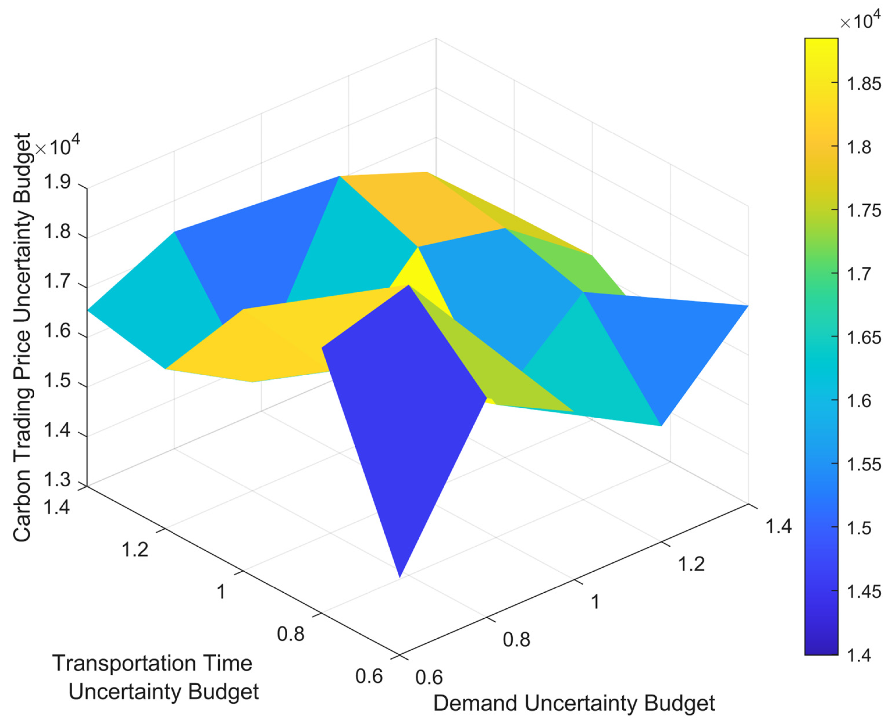
5.2.1. Analysis of the Impact of Uncertainty Budget Parameters

(1) Impact analysis of demand uncertainty

When both the transportation time and the carbon trading price uncertainty budget are at a relatively low level of 0.6, the uncertainty budget of demand increases from 0.6 to 1.4, the model always selects the route of “node 1-waterway-node 7-railway-node 17”, accounting for 100% in the five scenarios, as shown in

Table 5. Impact of demand uncertainty budget variations on route selection and cost.

${\mathrm{\Gamma }}_{\mathit{D}}$	${\mathrm{\Gamma }}_{\mathit{t}}$	${\mathrm{\Gamma }}_{\mathit{\alpha }}$	Optimal Route	Min. Cost (CNY)
0.6	0.6	0.6	1-Waterway-7-Railway-17	14,545.76
0.8	0.6	0.6	1-Waterway-7-Railway-17	17,411.26
1.0	0.6	0.6	1-Waterway-7-Railway-17	16,378.70
1.2	0.6	0.6	1-Waterway-7-Railway-17	15,324.08
1.4	0.6	0.6	1-Waterway-7-Railway-17	16,998.73

. The change in cost is as follows: It rises from CNY 14,545.76 to CNY 17,411.26, then drops to CNY 15,324.08, and finally rebounds to CNY 16,998.73. The increase in initial costs reflects the rise in capacity reserves caused by fluctuations in demand, leading to an increase in transportation and transshipment costs. The subsequent cost reduction indicates that the model has reduced some costs by optimizing the transportation plan, adjusting the transportation frequency and goods allocation. The recovery of terminal costs is due to the additional scheduling costs brought about by the extremely large fluctuations in demand. Overall, demand uncertainty mainly affects costs through changes in transportation capacity allocation, and its impact on specific route selection is relatively limited.

(2) Impact analysis of transportation time uncertainty

To reflect the moderate fluctuation of demand, the budget for demand uncertainty is set at 1.0, the budget for carbon trading price uncertainty remains at 0.6, and the budget for transportation time uncertainty is increased from 0.6 to 1.4. In most scenarios, the model still selects “node 1-waterway-node 7-railway-node 17” in most scenarios, as shown in

Table 6. Impact of transportation time uncertainty budget variations on route selection and cost.

${\mathrm{\Gamma }}_{\mathit{D}}$	${\mathrm{\Gamma }}_{\mathit{t}}$	${\mathrm{\Gamma }}_{\mathit{\alpha }}$	Optimal Route	Min. Cost (CNY)
1.0	0.6	0.6	1-Waterway-7-Railway-17	16,378.70
1.0	0.8	0.6	1-Waterway-12-Waterway-16-Railway-17	15,671.16
1.0	1.0	0.6	1-Waterway-7-Railway-17	18,004.49
1.0	1.2	0.6	1-Waterway-7-Railway-17	18,587.72
1.0	1.4	0.6	1-Waterway-7-Railway-17	14,222.07

. The cost first rises from CNY 16,378.70 to CNY 18,587.72. Then, with a route switch in the scenario, it decreases to CNY 15,671.16. Finally, when switching to the full railway route “node 1-railway-node 11-railway-node 17”, it drops to CNY 14,222.07. This indicates that after the uncertainty of transportation time increases, the initial cost rises, mainly due to the increase in time penalty cost. When the model adjusts the route and adds railways or other transportation modes with higher time stability, it can effectively alleviate the cost pressure caused by time fluctuations.

(3) Impact analysis of carbon trading price uncertainty

To simulate a more complex and realistic scenario, the budget for demand uncertainty is 1.2 and the budget for transportation time uncertainty is 1.0. As the carbon trading price uncertainty budget increases from 0.6 to 1.4, the model selects “node 1-waterway-Node 7-railway-node 17” in three scenarios, as shown in

Table 7. Impact of carbon trading price uncertainty budget variations on route selection and cost.

${\mathrm{\Gamma }}_{\mathit{D}}$	${\mathrm{\Gamma }}_{\mathit{t}}$	${\mathrm{\Gamma }}_{\mathit{\alpha }}$	Optimal Route	Min. Cost (CNY)
1.2	1.0	0.6	1-Waterway-7-Railway-17	17,625.40
1.2	1.0	0.8	1-Waterway-12-Waterway-16-Railway-17	17,488.58
1.2	1.0	1.0	1-Waterway-7-Railway-17	16,666.34
1.2	1.0	1.2	1-Waterway-12-Waterway-16-Railway-17	16,877.21
1.2	1.0	1.4	1-Waterway-7-Railway-17	16,909.49

. The cost initially decreases from CNY 17,625.40 to CNY 16,666.34, and then rises slightly to CNY 16,909.49. When the uncertainty budget of the carbon trading price is 0.80, the route switches to “node 1-waterway-node 12-waterway-node 16-railway-node 17”, reducing the fluctuation of carbon emission costs and achieving cost reduction. When the carbon budget is 1.2, the model again selects “node 1-waterway-node 12-waterway-node 16-railway-17”, further increasing the proportion of waterway to reduce the fluctuation risk. The uncertainty of carbon trading price prompts the model to adopt a dynamic route adjustment strategy to balance economic and environmental costs at different levels and reduce overall risks.

5.2.2. Comparative Analysis of Typical and Extreme Scenarios

In order to further explore the combined effect of uncertain factors, based on the value range (0.6 to 1.4) of uncertainty budgets for demand, transportation time and carbon trading price, eight typical and extreme scenarios are selected to analyze the changing trends of route selection and costs under different combinations of uncertainties. A typical scenario refers to a state where the uncertainty factors are at a medium or a single high level, which is a common and representative combination of uncertainties in the transportation system. Extreme scenarios refer to the state where the uncertainty factors are at extremely low or extremely high levels, which are the boundary conditions faced by the transportation system. The results are shown in

Table 8. Route selections and costs in typical and extreme scenarios.

No.	Scenario	${\mathrm{\Gamma }}_{\mathit{D}}$	${\mathrm{\Gamma }}_{\mathit{t}}$	${\mathrm{\Gamma }}_{\mathit{\alpha }}$	Optimal Route	Min. Cost (CNY)
1	Low Uncertainty	0.6	0.6	0.6	1-Waterway-7-Railway-17	14,545.76
2	High Uncertainty	1.4	1.4	1.4	1-Waterway-7-Railway-17	18,070.30
3	High Demand Uncertainty	1.4	0.6	0.6	1-Waterway-7-Railway-17	16,998.73
4	High Time Uncertainty	0.6	1.4	0.6	1-Waterway-12-Waterway-16-Railway-17	17,373.90
5	High Carbon Trading Price Uncertainty	0.6	0.6	1.4	1-Waterway-12-Waterway-16-Railway-17	16,080.56
6	High Demand and High Time Uncertainty	1.4	1.4	0.6	1-Waterway-7-Railway-17	16,282.30
7	High Time and High Carbon Price Uncertainty	0.6	1.4	1.4	1-Waterway-12-Waterway-16-Railway-17	17,022.51
8	High Demand and High Carbon Price Uncertainty	1.4	0.6	1.4	1-Waterway-7-Railway-17	17,771.81

.

(1) Comparison of low and high uncertainty scenarios

Scenario 1 is a low-uncertainty scenario, where all uncertainty budgets are at the lowest level. The optimal route is “node1-waterway-node7-railway-node17”, and the cost is CNY 14,545.76. This route combines the low-cost advantage of waterway transportation with the stability of railway transportation and is suitable for situations where the overall environmental fluctuations are relatively small. Scenario 2 is a highly uncertain scenario. The uncertainty budgets are all at the highest level. The route remains unchanged, but the cost rises to CNY 18,070.30, an increase of 24.2% compared with scenario 1. The simultaneous increase in three uncertainties has expanded the range of demand fluctuations, raised the time penalty cost, and exacerbated the fluctuations in carbon emission cost, resulting in a significant rise in the total cost. However, the route selection remains stable, indicating that in the overall transportation network, this route has a strong adaptability to uncertain factors and can maintain robustness in the case of large cost fluctuations.

(2) Single high uncertainty scenario analysis

The optimal route of scenario 3 is “node 1-waterway-node 7-railway-node 17”, and the transportation cost is CNY 16,998.73, which is 16.8% higher than that of scenario 1. The expansion of the fluctuation range of demand has increased the demand for transportation capacity and related costs, but the route remains unchanged, indicating that it has strong robustness when dealing with demand uncertainty. In scenario 4, the optimal route is adjusted to “node 1-waterway-node 12-waterway-node 16-railway-node 17”, and the transportation cost is CNY 17,373.9, an increase of 19.4% compared with scenario 1. When time uncertainty increases, waterway transportation is preferred to reduce the impact of time fluctuations, while the stability of railway transportation is utilized to further control the total cost. In scenario 5, the optimal route is the same as that in scenario 4, and the transportation cost is CNY 16,080.56, an increase of 10.5% compared with scenario 1. When the uncertainty of carbon trading price increases, there is a greater tendency to choose low-carbon waterway transportation to balance cost fluctuations.

(3) Double high uncertainty scenario analysis

Scenarios 6 to 8 explore the adjustment strategies for route selection and costs when two uncertain factors change simultaneously. In scenario 6, with high demand and high time uncertainty, the route remains at “node 1-waterway-node 7-railway-node 17”, and the cost rises to CNY 16,282.30, an increase of 11.9% compared with the low uncertainty scenario. After the simultaneous increase in demand and time uncertainty, the fluctuation range of transportation capacity demand and time expands, but the route remains unchanged, indicating that this route can balance the uncertainties of demand and time to a certain extent. By optimizing the transportation plan and rationally allocating the volume of goods and the frequency of transportation, the demand for transportation capacity and the cost of time penalty are reduced, enabling this route to still maintain good robustness in the case of increased uncertainty.

In scenario 7, with high time and high carbon trading price uncertainty, the optimal route is adjusted to “node 1-waterway-node 12-waterway-node 16-railway-node 17”, and the cost increases to CNY 17,022.51, an increase of 16.9% compared with the low uncertainty scenario. The combined effect of the uncertainty of time and carbon trading prices makes the transportation system need to make a trade-off between the time cost and the carbon emission cost. The stability of railway transportation reduces the time penalty cost, while the lower carbon emission level helps to control the fluctuation of carbon cost.

In scenario 8, under the circumstances of high demand and high carbon trading price uncertainty, the route remains at “node 1-waterway-node 7-railway-node 17”, but the cost rises to CNY 17,771.81, an increase of 22.2% compared with the low uncertainty scenario. The expansion of the fluctuation range of demand has put forward higher requirements for the demand of transportation capacity, and the fluctuation of carbon emission costs has intensified, leading to a further increase in costs. It also indicates that this route can provide a better balance between carbon emissions and transportation capacity reserves, enabling it to have strong adaptability even under highly uncertain conditions.

It can be seen that under the interaction of uncertain factors, the mechanism of route selection is different. When both demand and time uncertainties are relatively high, the model prioritizes maintaining route stability to ensure the feasibility of the transportation plan and the controllability of costs. When the uncertainty of time and the uncertainty of carbon trading price are superimposed, the model pays more attention to the fluctuation of carbon costs and selects the route with a higher proportion of railways to reduce the impact of carbon emission costs. When both the uncertainty of demand and the uncertainty of carbon trading price rise simultaneously, the model places more emphasis on cost minimization, optimizing transportation capacity reserves and carbon emission to reduce fluctuations in total costs.

5.2.3. Route Robustness Analysis

For 125 groups of uncertain scenarios, the frequency and proportion of the optimal route were statistically analyzed to evaluate the stability and adaptability of the route. The results are shown in

Table 9. Frequency and proportion of optimal route under different uncertainty scenarios.

Optimal Route	Frequency	Proportion (%)
1-Waterway-7-Railway-17	91	72.8
1-Waterway-12-Waterway-16-Railway-17	14	11.2
1-Waterway-12-Railway-16-Railway-17	12	9.6
1-Railway-11-Railway-17	5	4.0
1-Waterway-12-Waterway-16-Highway-17	2	1.6
1-Waterway-12-Waterway-15-Waterway-16-Railway-17	1	0.8

.

Among all scenarios, “node 1-waterway-node 7-railway-node 17” emerges 91 times, accounting for 72.8%, and remains stable under different uncertainty scenarios. Under the scenario of low uncertainty, the cost of this route is CNY 14,545.76. Under the scenarios of high demand and high time uncertainty, the cost rises to CNY 16,282.30, and the increase is relatively controllable. This indicates that the route can still maintain superior economy and stability under various combinations of uncertainties, and the model has strong robustness in route selection.

When the uncertain factors change significantly, the route selection will be adjusted. Under the scenario of high-time uncertainty, the route switches to “node 1-waterway-node 12-waterway-node 16-railway-node 17”. The frequency of this route is 14 times, accounting for 11.2%. The model tends to choose a more flexible route to reduce the time penalty cost. Under the scenario of high carbon trading price uncertainty, the route is adjusted to “node 1-waterway-node 12-railway-node 16-railway-node 17”, and the frequency of this route is 12 times, accounting for 9.6%. This indicates that in the case of large fluctuations in carbon trading price, the model is more inclined to choose the transportation mode with lower carbon emissions to reduce the fluctuations in carbon costs. The model can flexibly adjust the route according to different sources of uncertainty to reduce costs and maintain the stability of the transportation system.

Overall, this model shows strong robustness in an uncertain environment. When uncertainty intensifies, the model can reduce the time penalty cost and carbon cost through route adjustment, demonstrating strong adaptability. The optimization results are not only robust but also have the ability to be flexibly adjusted, which can effectively support decision-makers in formulating reasonable transportation plans in complex environments.

5.2.4. Algorithm Comparative Analysis

To verify the effectiveness of the genetic-simulated annealing hybrid algorithm, in this study, focusing on the multiple uncertainties of demand, transportation time and carbon price fluctuations, multiple tests are conducted, respectively, using the genetic algorithm (GA), the simulated annealing algorithm (SA) and the hybrid algorithm. The performance differences of each algorithm under uncertain disturbances are investigated from the dimensions of average cost, fluctuation range of solutions and stability, and the results are shown in Figure 5.

It can be seen that the optimization performances of GA, SA and the hybrid algorithm are significantly different. The average cost of GA is CNY 27,839.02, with a standard deviation of 6390.90. It is relatively stable but fluctuations still exist. The average cost of SA is as high as CNY 120,221.39, with a standard deviation of 69,234.78, showing significant instability and local trap problems. The hybrid algorithm shows better solutions and higher stability with an average cost of CNY 19,797.13 and a standard deviation of 1735.88. From the perspective of the trend curve, the cost of the hybrid algorithm remains at a relatively low level. By combining the advantages of GA global search and SA local tuning, it effectively addresses the uncertainties in demand, transportation time, and carbon trading price. The comprehensive performance indicates that the hybrid algorithm has better performance in complex scenarios and is suitable for multimodal transportation route selection.

6. Conclusions

This study focuses on the optimization of multimodal transportation routes, with a particular emphasis on the overall impact of uncertainties in demand, transportation time, and carbon trading price on scheme selection. By using the Box set to describe the upper and lower limit fluctuations of parameters and combining uncertain budget parameters to construct a hybrid robust stochastic optimization model, a route selection strategy that can maintain stability and efficiency under external environmental fluctuations is proposed. The research results show that different types of uncertainties affect the selection of transportation routes in different ways. That is, demand uncertainty mainly affects the allocation of transportation capacity and cost structure, the uncertainty of transportation time increases the time penalty cost, and the uncertainty of carbon trading prices encourages the choice of low-emission transportation modes. Although the cost will increase under high uncertainty, the model can still provide a stable solution. Compared with the traditional genetic algorithm (GA) and simulated annealing algorithm (SA), the hybrid algorithm of the two shows superior performance in terms of cost control and solution stability. Evidently, robust optimization can effectively deal with the problem of multimodal transportation route selection where the parameter values are uncertain and the distribution is unknown. Moreover, the robustness of the optimization model is adjustable, supporting decision-makers to weigh optimality and robustness according to their preferences and obtain solutions that take into account both economic and environmental benefits, which is conducive to the development of sustainable transportation.

There are still some limitations in this study. The model’s depiction of uncertainty is mainly based on Box uncertain sets, scenarios, and uncertain budget parameters, without considering the correlations among uncertainty parameters. In the future, more flexible or distributed assumptions can be considered to expand the scope of the application. Sudden factors such as weather and equipment failure are not taken into account, and the emergency situations in actual transportation can be further studied. Furthermore, the situation of insufficient transportation capacity was not considered. In future research, transportation capacity constraints can be incorporated into the model and an adaptive routing mechanism can be developed to better cope with the impact brought by transportation capacity limitations. In addition, more efficient intelligent solution algorithms can be explored to further enhance the model’s performance in terms of solution speed and result quality. Overall, this paper conducts a beneficial exploration of the robust optimization of multimodal transportation route selection in an uncertain environment, providing a reference for future sustainable transportation decision-making under dynamic situations and multi-factor interference.

References

1. Macioszek, E. Cargo transport on the example of a selected mode of transport in Poland. Sci. J. Sil. Univ. Technol. Series Transp. 2024, 122, 181–197. [Google Scholar] [CrossRef]
2. Zhang, H.; Li, Y.; Zhang, Q.; Chen, D. Route selection of multimodal transport based on China railway transportation. J. Adv. Transp. 2021, 2021, 9984659. [Google Scholar] [CrossRef]
3. Rouky, N.; Boukachour, J.; Boudebous, D.; Alaoui, A.E.H. Optimization under uncertainty: Generality and application to multimodal transport. Int. J. Supply Oper. Manag. 2023, 10, 223–244. [Google Scholar]
4. Wu, C.; Zhang, Y.; Xiao, Y.; Mo, W.; Xiao, Y.; Wang, J. Optimization of multimodal paths for oversize and heavyweight cargo under different carbon pricing policies. Sustainability 2024, 16, 6588. [Google Scholar] [CrossRef]
5. Sun, J.Q.; Wang, S.N.; Yan, S.X. Path selection of multimodal transport for refrigerated containers considering carbon emission. J. Dalian Marit. Univ. 2022, 48, 57–65. (In Chinese) [Google Scholar]
6. Li, H.F.; Hu, D.W.; Chen, X.Q.; Wang, Y. Expand hub location-routing problem for hybrid hub-and-spoke multimodal transport network considering carbon emissions. J. Traffic Transp. Eng. 2022, 22, 306–321. (In Chinese) [Google Scholar]
7. Laurent, A.B.V.S.V.D. CarbonRoadMap: A multicriteria decision tool for multimodal transportation. Int. J. Sustain. Transp. 2020, 14, 205–214. [Google Scholar] [CrossRef]
8. Yang, L.; Zhang, C.; Wu, X. Multi-objective path optimization of highway-railway multimodal transport considering carbon emissions. Appl. Sci. 2023, 13, 4731. [Google Scholar] [CrossRef]
9. Li, M.; Sun, X. Path optimization of low-carbon container multimodal transport under uncertain conditions. Sustainability 2022, 14, 14098. [Google Scholar] [CrossRef]
10. Peng, Y. Research on green multimodal transportation path optimization based on distributionally robust chance constraints with uncertain demand. In Proceedings of the Eighth International Conference on Traffic Engineering and Transportation System (ICTETS 2024), Dalian, China, 20–22 September 2024; SPIE: Bellingham, WA, USA, 2024; Volume 13421, pp. 1666–1676. [Google Scholar]
11. Liu, Z.; Zhou, S.; Liu, S. Optimization of multimodal transport paths considering a low-carbon economy under uncertain demand. Algorithms 2025, 18, 92. [Google Scholar] [CrossRef]
12. Peng, Y.; Yong, P.; Luo, Y. The route problem of multimodal transportation with timetable under uncertainty: Multi-objective robust optimization model and heuristic approach. RAIRO Oper. Res. 2021, 55, S3035–S3050. [Google Scholar] [CrossRef]
13. Wang, T.; Dai, C.; Li, H.; Wu, R. Multimodal Transportation Routing Optimization Considering Schedule Constraints and Uncertain Time. IAENG Int. J. Appl. Math. 2024, 54, 2656–2668. [Google Scholar]
14. Guo, J.; Liu, T.; Song, G.; Guo, B. Solving the robust shortest path problem with multimodal transportation. Mathematics 2024, 12, 2978. [Google Scholar] [CrossRef]
15. Zhang, X.; Jin, F.Y.; Yuan, X.M.; Zhang, H.Y. Low-carbon multimodal transportation path optimization under dual uncertainty of demand and time. Sustainability 2021, 13, 8180. [Google Scholar] [CrossRef]
16. Li, L.; Zhang, Q.; Zhang, T.; Zou, Y.; Zhao, X. Optimum route and transport mode selection of multimodal transport with time window under uncertain conditions. Mathematics 2023, 11, 3244. [Google Scholar] [CrossRef]
17. Peng, X.; Heng, Z.; Xi, C. Optimization of intermodal routes for reefer containers under double uncertainty. In E3S Web of Conferences; EDP Sciences: Les Ulis, France, 2024; Volume 512, p. 03015. [Google Scholar]
18. Li, X.; Sun, Y.; Qi, J.; Wang, D. Chance-constrained optimization for a green multimodal routing problem with soft time window under twofold uncertainty. Axioms 2024, 13, 200. [Google Scholar] [CrossRef]
19. Hou, D.N.; Liu, S.C. Optimization of cold chain multimodal transportation routes considering carbon emissions under hybrid uncertainties. Artif. Intell. 2024, 32, 2243–2256. [Google Scholar] [CrossRef]
20. Sun, Y. Green and reliable freight routing problem in the road-rail intermodal transportation network with uncertain parameters: A fuzzy goal programming approach. J. Adv. Transp. 2020, 2020, 7570686. [Google Scholar] [CrossRef]
21. Xu, Z.; Zheng, C.; Zheng, S.; Ma, G.; Chen, Z. Multimodal transportation route optimization of emergency supplies under uncertain conditions. Sustainability 2024, 16, 10905. [Google Scholar] [CrossRef]
22. Han, W.; Chai, H.; Zhang, J.; Li, Y. Research on path optimization for multimodal transportation of hazardous materials under uncertain demand. Arch. Transp. 2023, 67, 91–104. [Google Scholar] [CrossRef]
23. Zhu, C.; Zhu, X. Multi-objective path-decision model of multimodal transport considering uncertain conditions and carbon emission policies. Symmetry 2022, 14, 221. [Google Scholar] [CrossRef]
24. Zhang, J.; Li, H.; Han, W.; Li, Y. Research on optimization of multimodal hub-and-spoke transport network under uncertain demand. Arch. Transp. 2024, 70, 137–157. [Google Scholar] [CrossRef]
25. Gao, X.; Yao, J.; Liu, H. Path Optimization of Multimodal Transport Models under Carbon Tax Policy. In Proceedings of the International Conference on Traffic and Transportation Studies, Singapore, 10–12 July 2024; Springer Nature: Singapore, 2024; pp. 427–434. [Google Scholar]
26. Reşat, H.G.; Türkay, M. Design and operation of intermodal transportation network in the Marmara region of Turkey. Transp. Res. Part E Logist. Transp. Rev. 2015, 83, 16–33. [Google Scholar] [CrossRef]
27. Zhang, T.; Cheng, J.; Zou, Y. Multimodal transportation routing optimization based on multi-objective Q-learning under time uncertainty. Complex Intell. Syst. 2024, 10, 3133–3152. [Google Scholar] [CrossRef]
28. Cao, Q.K.; Qin, M.N.; Ren, X.Y. Bi-level programming model and genetic simulated annealing algorithm for inland collection and distribution system optimization under uncertain demand. Adv. Prod. Eng. Manag. 2018, 13, 147–157. [Google Scholar] [CrossRef]
29. Shao, Y.; Han, X.L.; Cao, L.J. Optimization of multimodal transport path considering carbon policy. In Proceedings of the Sixth International Conference on Traffic Engineering and Transportation System (ICTETS 2022), Chengdu, China, 22–24 July 2022; Edited by SPIE. SPIE: Bellingham, WA, USA, 2023; pp. 728–736. [Google Scholar]
30. Zhao, F.; Zeng, X. Optimization of transit network layout and headway with a combined genetic algorithm and simulated annealing method. Eng. Optim. 2006, 38, 701–722. [Google Scholar] [CrossRef]
31. Cheng, X.; Jin, C.; Yao, Q.; Wang, C. Robust optimization study on multimodal transportation route selection under carbon trading policy. Chin. Manag. Sci. 2021, 29, 82–90. [Google Scholar]
Figure 1. Example of a multimodal transportation network.
Sustainability 17 05508 g001
Figure 2. Hybrid optimization algorithm process for multimodal transportation route under multiple uncertainties.
Sustainability 17 05508 g002
Figure 3. Multimodal transportation network in the case.
Sustainability 17 05508 g003
Figure 4. Comprehensive impact of uncertain budget parameters on the cost of the optimal route.
Sustainability 17 05508 g004
Figure 5. Algorithm comparison.
Sustainability 17 05508 g005