Article

Impacts of Landscape Mosaic Patterns on Habitat Quality Using OLS and GWR Models in Taihang Mountains of Hebei Province, China

1
College of Landscape Architecture and Tourism, Hebei Agricultural University, Baoding 071000, China
2
School of Life Sciences, Sun Yat-Sen University, Guangzhou 511400, China
3
Hebei Key Laboratory of Floral Biological Breeding, Hebei Agricultural University, Baoding 071000, China
4
School of Landscape Architecture, Beijing Forestry University, Beijing 100083, China
*
Author to whom correspondence should be addressed.
These authors contributed equally to this work.
Sustainability 2025, 17(12), 5503; https://doi.org/10.3390/su17125503
Submission received: 10 April 2025 / Revised: 28 May 2025 / Accepted: 10 June 2025 / Published: 14 June 2025

Abstract

:
Based on the fundamental principles of spatial heterogeneity and landscape ecology, landscape mosaic (LM) offers a more effective method for capturing variations in landscape spatial components, patterns, and ecological functions compared to land use and land cover (LULC). This advantage is particularly pronounced when employing the InVEST model to evaluate habitat quality (HQ), as field surveys often yield highly variable results that challenge the accuracy and applicability of LULC-based assessments. This paper focuses on the Taihang Mountain area in Hebei Province as the study region, utilizing the Principal Component Analysis (PCA), Self-Organizing Map (SOM), and Euclidean Distance (ED) model to achieve LM classification of the area. Based on this, the InVEST-HQ assessment is conducted, employing both OLS and GWR models to analyze the correlation between HQ and LM landscape patterns. The results indicate that (1) seven major LULC types were reclassified into nine pillar LM types and eleven transitional LM types, with a significant number of ecotone types emerging between different LULC types, among which cultivated land plays the most prominent role; (2) from 2000 to 2020, the overall HQ in the study area exhibited a continuous deterioration trend, particularly marked by a notable increase in functional areas of HQ areas classified as Level I; (3) factors such as the complexity of patch edges, the continuity between patches, and the diversity of patch types all significantly impact HQ. This study introduces an innovative methodological framework for HQ assessment using LM classifications within InVEST model, offering a robust foundation for comprehensive biodiversity monitoring and informed ecological management in the study area.

1. Introduction

Habitat quality (HQ) refers to an ecosystem’s ability to provide suitable conditions for the survival of organisms, reflecting local biodiversity levels as well as the integrity and diversity of regional ecosystem functions [1,2,3]. HQ assessment methods are widely used as proxy indices for biodiversity in academic research. They provide insights into biological habitats in target regions and reveal the effects of ecological protection and restoration policies, urbanization, climate change, and other factors on biodiversity [4,5,6].
Broadly, HQ assessment methods can be categorized into two types. The first is field investigation-based methods, which primarily focus on specific species [1]. While these methods are highly targeted, they are also time-consuming, labor-intensive, and generally suited for small-scale field studies [7]. The second type comprises model-based methods, such as Social Values for Ecosystem Services (SoIVES) [8], Artificial Intelligence for Ecosystem Services (ARIES) [9], Multi-scale Integrated Models of Ecosystem Services (MIMES) [10], and Integrated Valuation of Ecosystem Services and Tradeoffs (InVEST) [11,12]. Among them, the “HQ” module in the InVEST model (InVEST-HQ) is the most advanced and widely applied [5,12]. The InVEST-HQ assessment has been employed to study diverse natural environments, including mountains, plains, and river basins [12,13], as well as varying scales such as states, cities, and counties [14,15,16]. A critical parameter in the InVEST model is land use/land cover (LULC), which establishes a quantitative relationship between habitats and threats [17]. However, some scholars argue that the model’s heavy reliance on LULC data introduces limitations, as variations in LULC can significantly influence habitat quality assessment results [18]. Combining LULC with factors such as terrain, climate, vegetation, and urbanization often better explains HQ changes [3,19]. These findings highlight potential shortcomings when HQ assessments rely solely on LULC.
From a landscape ecology perspective, the migration paths and habitat preferences of organisms are often more susceptible to the influences of the landscape mosaic (LM), which encompasses various elemental attributes, including the matrix and the patches within it [20,21]. In the context of biodiversity conservation, both patches and corridors within the LM are particularly significant. The interplay of climate, topography, and plant resources generates a complex mosaic [20,22]. LM views land space as a highly heterogeneous composite ecosystem, incorporating natural, social, and economic factors [23]. In contrast, land use (LU) emphasizes land development, management, and socio-economic attributes, while land cover (LC) focuses on the types of natural or artificial surface elements [24]. Based on the aforementioned content, it can be argued that the introduction of LM instead of LULC into InVEST-HQ assessments can better capture the heterogeneity of land space in terms of composition and configuration, thereby improving the alignment of HQ assessment results with real-world conditions. LM, as conceptualized by renowned landscape ecologists like Forman [22] and Naveh [25], represents a typological depiction of landscape elements or ecosystem sources at the landscape scale. Numerous studies have demonstrated a close relationship between LM and HQ, with LM outperforming LULC in several respects. These findings can be categorized into two key patterns [26]: (1) Compositional Heterogeneity (CPH): CPH influences the capacity of LM to support biological survival. Landscapes comprising multiple ecological elements generally exhibit higher habitat suitability than those dominated by a single element. For instance, woodland-cultivated land mosaics and grassland-cultivated land mosaics support greater diversity in surface arthropods and plant communities than cultivated land patches alone [27]. Similar trends have been observed in forest-steppe mosaics and aquatic-terrestrial mosaics [28,29]. Additionally, socio-economic factors like population density and GDP can influence the impact of urban construction areas with identical LULC attributes on biodiversity [30]. (2) Configurative Heterogeneity (CFH): CFH refers to the spatial patterns of LM, including fragmentation, diversity, and connectivity, which significantly affect biodiversity levels [31]. This is particularly evident in transition regions between adjacent heterogeneous patches. The stability of transitional landscape mosaics (TLMs) influences the transmission and filtration efficiency of ecological flows across ecological boundaries, making these areas critical for constructing biological migration corridors [32,33]. Overall, in the past few decades, particularly from the late 1990s to the early 21st century, there has been a growing interest in the classification of landscape mosaics, their spatiotemporal evolution, and their impact on ecosystem service functions [34,35,36,37,38,39,40]. Nevertheless, compared to the research outcomes based on LULC classification systems, the academic achievements related to ecosystem services based on LM remain relatively scarce. This highlights a significant contrast for argumentation between the two fields. Additionally, an indirect consequence is that many findings from field investigations remain disconnected from the results of HQ model assessments.
The integrity and rationality of LM classification are crucial for improving the accuracy of HQ assessment results. LM classification typically involves dividing land into equally sized grid units, representing the spatial distribution of natural or man-made elements associated with LULC types. Using quantitative spatial clustering analysis, the land grid is classified based on the spatial mosaic relationships of these elements [41]. Currently, commonly used LM classification models include Landscape Pattern Types (LPTs), Land Units (LUs), Matrix of Landscape Types (MLT), and the Tri-Polar Model (TPM), among others [41,42,43]. Among these, the TPM is widely applied [44]. Inspired by the “soil triangle” principle, the TPM classifies LM into three ecosystem types: natural, agricultural, and built-up areas. Vizzari et al. [35] introduced the concept of a neighborhood mosaic in their study of transitional landscapes, offering innovative approaches to LM classification. Vizzari et al.’s approach used ISODATA clustering to reclassify LMs and allows for the flexible selection of spatial classification elements, making it adaptable and expandable for LM classification studies. However, the TPM struggles to support the classification process of landscape mosaics that exceed three types of ecosystem types. The ISODATA model is currently mainly applied to the classification exploration of landscape mosaics at a specific time. In order to facilitate the comprehensive classification of multiple factors and various time periods, the Self-Organizing Map (SOM) model is introduced as a solution. SOM, an unsupervised competitive neural network with adaptive, self-organizing, and self-learning capabilities, has been widely applied in studies of ecosystem service bundles and landscape classification [45,46].
Numerous studies indicate that LULC changes significantly and complexly impact HQ, highlighting the importance of exploring the relationship between LULC changes and HQ [5,47,48]. Current methods for studying this relationship include various models such as the Pearson coefficient [49], Spearman coefficient [50], Ecological Contribution (EC) [51], Ordinary Least Squares (OLS) [4], Geographical Detector (GD) [52], and geographically weighted regression (GWR) [53]. Among these, OLS and GWR have become the more commonly used models in recent years and are often employed together to analyze the impacts of LULC, landscape patterns, and both natural and socio-economic factors on HQ [4,54]. The OLS model identifies the optimal functional fit for data by minimizing the sum of squared errors, thereby providing an efficient method to quantify the correlations between variables from a mathematical statistics perspective [55]. However, the OLS model may overlook the spatial non-stationarity of geographical factors, potentially leading to biased results or inefficient estimations [56]. In contrast, the GWR model is a statistical approach that captures the spatial characteristics of relationships by accounting for spatial heterogeneity through the construction of local regression equations at each grid. This model can provide more comprehensive spatial correlation information between multiple variables in HQ [53].
For our case study, we selected the Taihang Mountains in Hebei Province. As essential parts of terrestrial ecosystems, mountainous areas are rich in biodiversity with a high value of ecosystem productivity [57]. However, mountainous ecosystems are inherently fragile and are particularly susceptible to the impacts of urbanization and human activities [5]. The Taihang Mountains are a significant and representative mountain range in China. This range spans four provinces and municipalities: Hebei, Beijing, Shanxi, and Henan. The section of the Taihang Mountains located in Hebei Province, situated in the eastern part of the range, serves as an ecological barrier to the development of the Beijing–Tianjin–Hebei urban agglomeration. Over the past 20 years, urbanization has led to extensive LULC changes in this area, threatening the originally rich yet fragile mountain ecosystem [58]. Consequently, this region presents an excellent case study for exploring ecosystem heterogeneity and the resulting spatiotemporal evolution of HQ. This study aims to achieve the following objectives: (1) Discuss the landscape heterogeneity and its spatiotemporal evolution in the Taihang Mountains of Hebei Province through LM classification analysis. (2) Utilize LM classification results instead of LULC to conduct HQ evaluation. (3) Apply OLS and GWR to explore the quantitative relationship between the LM pattern and HQ. Then, we propose strategies for improving biodiversity in the Taihang Mountains of Hebei Province.

2. Materials and Methods
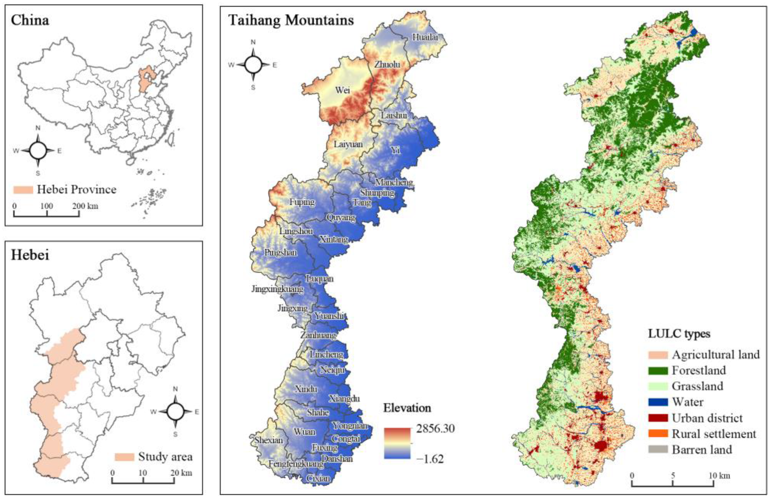
2.1. Study Area

The Taihang Mountains in Hebei Province (34°34′–40°43′ N, 110°14′–114°33′ E) are situated in the western part of the province (Figure 1). The study area exhibits a northeast–southwest alignment and resembles a strip, spanning 32 counties across five cities—Baoding, Shijiazhuang, Xingtai, Handan, and Zhangjiakou—covering a total area of 39,507.93 km2. This mountain range lies within the transition zone between China’s second and third-level landform terraces, with most peaks rising above 1200 m above sea level. The topography is characterized by higher elevations in the north and west, and lower elevations in the south and east. Climatically, the region experiences a warm temperate semi-humid continental monsoon climate, with an average annual temperature of approximately 10 °C and annual rainfall averaging around 550 mm. In terms of ecological resources, this area serves as a significant ecological source in Hebei Province, boasting a rich diversity of animal and plant life. However, the Taihang Mountains are also recognized as ecologically fragile areas [5]. The unique meteorological conditions, coupled with a large population and rapid urbanization, contribute to the instability of the ecosystem in this region. The Chinese government recognizes mountainous areas as a fundamental component of the overall ecological spatial pattern in Hebei Province. To protect biodiversity and enhance water source conservation, it has initiated ecological protection and restoration projects focusing on mountains, water, forests, fields, lakes, and grasslands. To ensure sustainability in policy implementation, it is essential to identify the landscape heterogeneity within the region and investigate the effects of the landscape pattern on biological habitats.

2.2. Theoretical Framework

The main components of this study include the following: (1) LM classification (Figure 2). Initially, basic data such as LULC, digital elevation model (DEM), and socio-economic factors are collected to extract the LM classification factors. The LM classification factors utilized in this study consist of four major categories: natural environment, plant resources, urban and rural development, and socio-economic and population factors. Subsequently, we integrate the Principal Component Analysis (PCA), Self-Organizing Map (SOM), and Euclidean Distance (ED) models, and incorporate the selected factors for classification to obtain the LM classification results. (2) InVEST-HQ assessment. This study utilizes the LM classification results as a substitute for LULC in the InVEST-HQ assessments and examines the changes in the habitat quality index over the study period. (3) OLS and GWR correlation analysis. Utilizing OLS and GWR models, this paper investigates the impact of four LM pattern indices—FRAC_MN, SPLIT, CONTAG, and SHDI—on the habitat quality index. Based on these findings, a landscape ecological planning strategy aimed at biodiversity protection and enhancement is proposed.

2.3. Data Sources

In this study, the data utilized include LULC, DEM, nighttime light index, and socio-economic data, among others. All data sources, formats, and processing procedures are presented in Table 1. LULC is the most important foundational data in this study. We have obtained data for the years 2000, 2010, and 2020. The data utilized is a national-scale, multi-period land use/land cover remote sensing detection database established by the Chinese Academy of Sciences, based on the National Resources and Environment Database and primarily leveraging U.S. Landsat remote sensing imagery [59]. The LULC data is characterized by high accuracy and robust applicability, with a spatial resolution of 30 m and an overall accuracy exceeding 90% [60,61], having been validated by research in various domains, including urban expansion [62], land prediction [63], and ecosystem service assessment [64]. Throughout the research process, the aforementioned data were uniformly formatted to the WGS 1984-UTM Zone 50N coordinate system, maintaining a data resolution of 30 m (Table 1).
Figure 2. Theoretical framework for LM classification.
Sustainability 17 05503 g002

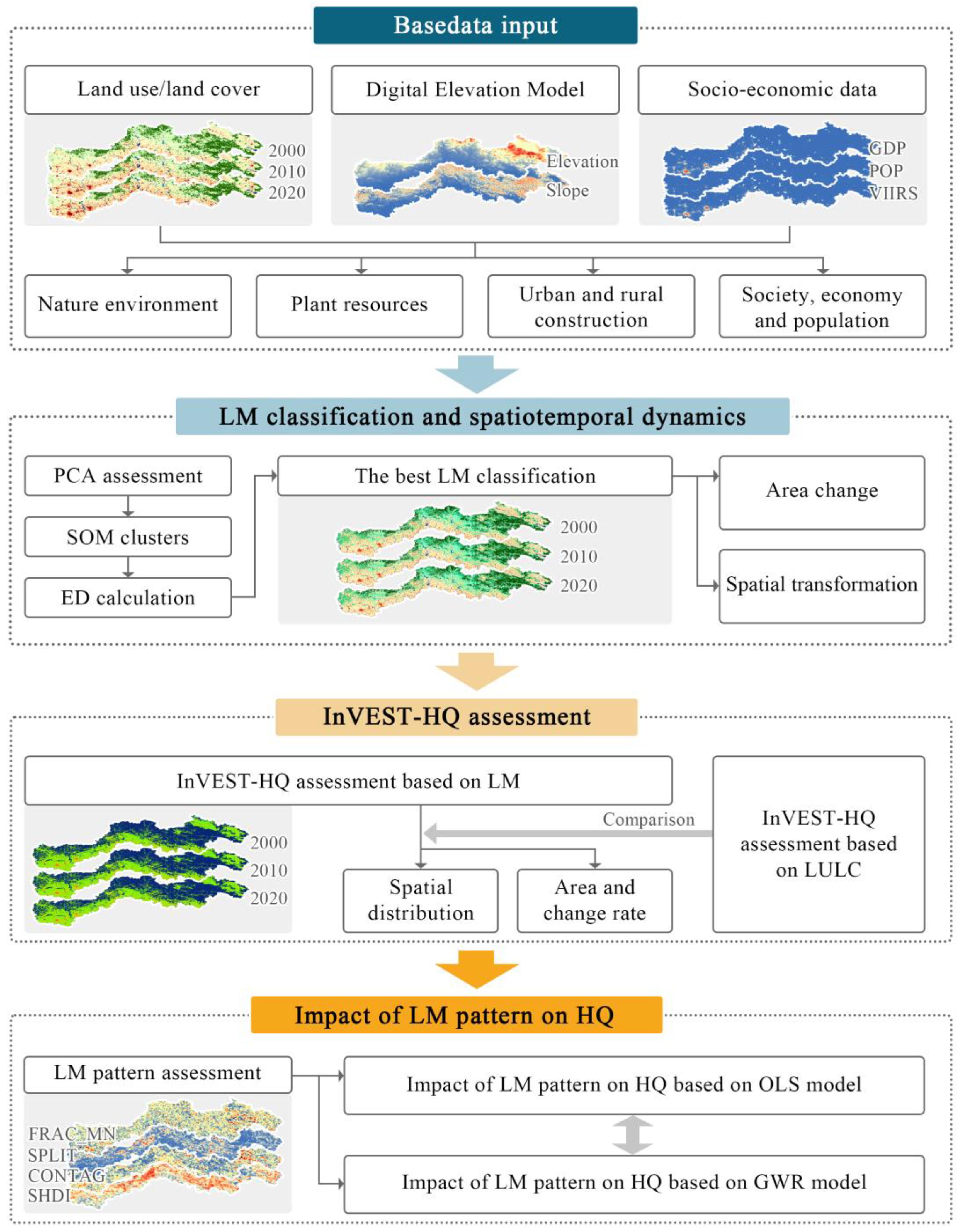
2.4. Research Method

We employed four sets of research methods to quantify the relationship between LM patterns and HQ indices in the study area, including LM classification, InVEST-HQ evaluation, LM pattern assessment, and their impact on InVEST-HQ evaluation results. PCA, SOM, and ED models were utilized for conducting LM classification, and the results of LM classification will serve as crucial foundational data to be imported into the InVEST-HQ model to obtain spatial quantification results of habitat quality in the study area. Meanwhile, the LM classification results will be input into FRAGSTATS 4.2 software to calculate typical landscape pattern indices. Finally, OLS and GWR models will be employed to assess the impact of LM pattern indices on habitat quality results from the perspectives of mathematical statistics and spatial differentiation.

2.4.1. Landscape Mosaic Classification

  • Index system
The primary objective of LM classification is to articulate the landscape heterogeneity of the study area. The selection of fundamental factors should comprehensively reflect the diversity of natural, urban, and rural elements within the site. Vizzari et al. proposed the urban–rural–natural gradient evaluation method, which employed the LULC macrotype derived from the CORINE Land Cover database [35]. They processed the data by converting points from the raster layer and conducted kernel density analysis. We build upon their research methods while expanding the range of basic factor types. Initially, the LM classification factor system was organized into four categories comprising twelve factors (Table 2). This includes seven first-level LULC types: water, agricultural land, forestland, grassland, bare land, urban districts, and rural settlements. For the processing of LULC data, we employed the ESRI ArcGIS 10.5 platform to convert the LULC raster layer into a regular point grid with a 30 m interval, aligning with the native resolution of the source data. Subsequently, kernel density evaluation technology was applied to transform values at specific locations into a continuous surface, with the bandwidth for the kernel density analysis set to 1000 m.
The LM classification system integrates a variety of natural, social, and economic environmental factors, including elevation, slope, nighttime light intensity, population density, and gross domestic product. These factors allow for a more nuanced refinement of the LM classification. As discussed in the analysis below, elevation and slope contribute to a detailed classification of agricultural land, forestland, and grassland. Simultaneously, nighttime light intensity and other variables offer valuable supplementary insights for the LM classification of urban districts and rural settlements.
2.
PCA assessment
In the LM classification process, redundancy among elements can lead to discrepancies between the classification outcomes and the actual conditions. To address this issue, we first divided the study area into 438,977 grids, employing a standard unit of 300 m × 300 m, and recorded the values of each factor system for the years 2000, 2010, and 2020. Subsequently, we utilized the IBM SPSS 23 Statistics platform to analyze the 12 factors, applying Principal Component Analysis to eliminate correlations and data redundancy. In all cases, the first eight principal components were selected, as they accounted for at least 90% of the variance.
3.
SOM cluster and ED assessment
To conduct LM classification analysis over multiple years, we utilized a SOM to identify LM within the study area. The SOM is an unsupervised competitive neural network characterized by its adaptive, self-organizing, and self-learning capabilities. It has been widely employed in studies related to geographical zoning and remote sensing image classification [70,71]. The SOM cluster analysis involves three steps: (1) utilizing the MATLAB R2019a platform to conduct the SOM cluster analysis by establishing the initial number of clusters; (2) employing ED assessment to compute the cluster sum of squares for each initial scenario and analyzing the resulting patterns to determine the optimal number of clusters; (3) importing the SOM clustering results into ESRI ArcGIS 10.5 for fishnet integration, which serves as the LM classification results. The criteria for assigning LM classification names are based on the methodology outlined by Vizzari et al. [35,68].

2.4.2. Habitat Quality Evaluation

InVEST 3.8.5 was selected to conduct habitat quality assessments. The InVEST model was developed by Stanford University, the World Wildlife Fund, and the Nature Conservancy, and it is a set of spatial models that analyze and predict the provision of ecosystem services and habitat provision, given LULC maps and related biophysical, economic, and institutional data for a given region, and quantitatively assesses habitat quality from a biodiversity perspective [72,73]. InVEST-HQ can establish various types of LULC by defining habitat suitability and considering LULC with intensive human activities as sources of biodiversity threats, along with their corresponding threat parameters. It also examines the quantitative relationships between habitats and threats to LULC. To enhance the consistency of model calculation results with real-world scenarios, we utilized LM classification results instead of LULC for HQ analysis. Additionally, we configured the parameter system by referencing the measured research outcomes of various representative LM biodiversity (Table 3 and Table 4) [27,28,29,74,75,76]. The InVEST-HQ is calculated as follows:
Q x j = H j 1 D x j z D x j z + k z
where Qxj is the habitat quality index, Hj represents the habitat suitability y of landscape mosaic type j, z and k are constants with a value of 2.5 and 0.5, respectively, and Dxj denotes the threat level in grid cell x with landscape mosaic type j.

2.4.3. Landscape Mosaic Pattern Metrics

The landscape pattern index serves as a highly condensed representation of spatial pattern information, reflecting the structure, composition, and spatial configuration of landscapes across multiple levels. FRAGSTATS 4.2 is a spatial pattern analysis program designed to quantify landscape structures. It effectively measures the spatial heterogeneity of landscapes, represented in either categorical maps or continuous surfaces. This approach has become increasingly common for quantifying landscape pattern indices [77,78]. It can be categorized into three main types: Patch, Class, and Landscape. In this study, we utilize LM rather than LULC to evaluate and analyze HQ. Consequently, it is essential to investigate whether there is a difference in the impact of LM on HQ compared to that of LULC. Building on existing research findings [79,80,81,82,83], we employed four land metrics with low correlation at the landscape level to represent the landscape mosaic pattern: the Mean Fractal Dimension Index (FRAC_MN), the Splitting Index (SPLIT), Contagion (CONTAG), and Shannon’s Diversity Index (SHDI). These four indices correspond to four dimensions, including shape, aggregation-subdivision, aggregation-interspersion, and diversity.

2.4.4. OLS and GWR Model

The OLS method is employed in this study as a means to evaluate the stability of factors influencing the habitat quality index. As a commonly used statistical method, the OLS model can elucidate the driving relationships between a single dependent variable and multiple independent variables. This study utilizes it to compute the fundamental regression relationship between the habitat quality index per unit area and various LM landscape pattern indices. The OLS model can be expressed as follows:
y i = β 0 + k = 1 p β k x i k + ε i
where yi denotes the HQ index at position i in the study area, β0 represents the square spatial intercept, βk is the regression coefficient of the k-th LM pattern index, xik is the value of the k-th LM pattern index at position i in space, and εi is the algorithm residual.
The OLS model is a linear non-spatial regression model designed to examine the relationship between independent and dependent variables across a broad area. However, its limitation lies in its inability to adequately capture the influence of driving factors on habitat quality at different locations within the study area. Consequently, after initially screening the driving factors using the OLS model, this study employed the GWR model to further assess the impact mechanisms of land use pattern factors on habitat quality from a spatial perspective. In contrast to the OLS model, the GWR model incorporates spatial distance weighting, resulting in evaluation outcomes that are more informative and reliable [84]. We utilizes OLS and GWR models to quantify the correlation between landscape patterns of LM and HQ indices. The primary aim is to understand the impact of LM landscape patterns on habitat quality from both a mathematical statistical and spatial differentiation perspective, while also comparing the computational results between global and local models. The GWR model can be expressed as follows:
y i = β 0 U i , V i + k = 1 n β k U i , V i x k ( U i , V i ) + ε i
β k U i , V i = X T W U i , V i X 1 X T W ( U i , V i ) y  
W i j = e x p ( d i j 2 / h 2 )
where β 0 ( U i ,   V i ) represents the geographically weighted regression intercept at the spatial location ( U i ,   V i ) and β k ( U i ,   V i ) denotes the weighted regression coefficient of the k independent variable (LM pattern index) at the spatial location ( U i ,   V i ) . The value of the k independent variable (LM pattern index) at the spatial location ( U i ,   V i ) is denoted as x k ( U i ,   V i ) , and ε k refers to the algorithm’s residuals. X T represents the transpose of the independent variables (LM pattern index), and W ( U i ,   V i ) is the distance weight matrix. The bandwidth based on the AIC criterion is denoted as h, and d i j is the distance between spatial locations i and j.
Before conducting OLS and GWR analyses, the analysis divided the study area image into a 3 km × 3 km grid using the Create Fishnet tool in ESRI ArcGIS 10.5. Subsequently, variables such as the landscape mosaic pattern index and habitat quality required for the study were aggregated into the grid.

3. Results

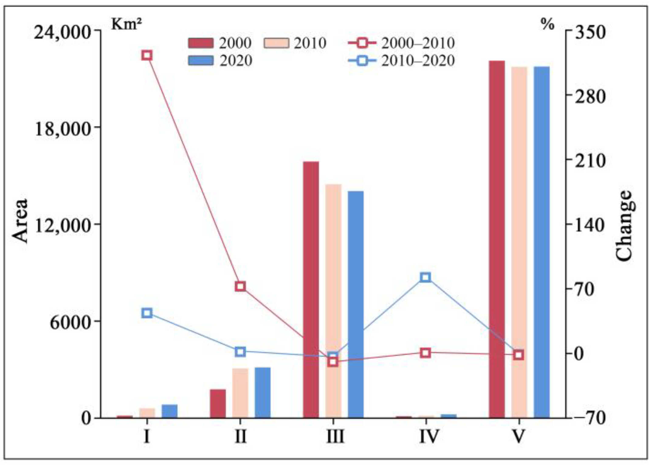
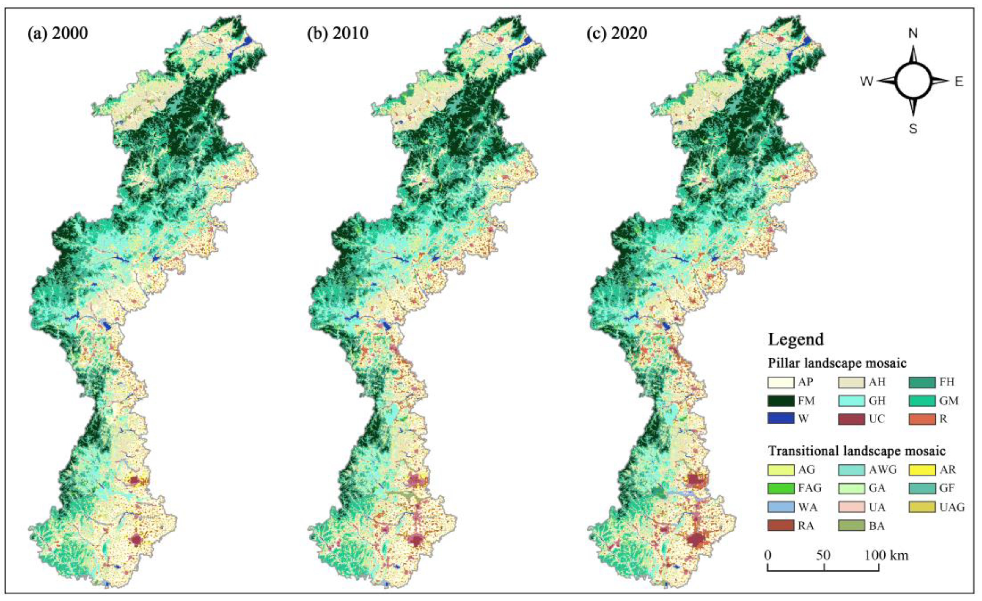
3.1. Classification of and Changes in Landscape Mosaic

3.1.1. Classification of Landscape Mosaic

As illustrated in Table 5 and Table A1, Table A2 and Table A3, the LM in the Taihang Mountains of Hebei Province is classified into two categories: pillar landscape mosaic (PLM) and transitional landscape mosaic (TLM). Regarding the definitions of PLM and TLM, we refer to the research methodology of Vizzari et al. [35,68], which defines an LM as a PLM when the area proportion of a particular LULC type is ≥75%, and as a TLM when the combined area proportion of two or more LULC types is ≥75%. The PLM can be further subdivided into nine types, while the TLM encompasses eleven types. Based on the classification criteria, the seven macro-level LULC types in the study area are categorized into a total of twenty LM types. Notably, with the exception of GF, all ten types of TLM incorporate elements of farmland landscapes, which suggests that there is a close interrelationship between farmland and most landscape spaces such as forest, grassland, water, urban districts, and rural settlement. This phenomenon is characteristic of most plain areas in China [85].
Figure 3 illustrates the spatial distribution of various types of LM from 2000 to 2020. APs are predominantly found in the eastern plain region of the study area, interspersed with UC and UA. AHs are located at the interface between mountainous and plain regions. Additionally, the northern basin of the study area features extensive areas of AH landscapes. In the mountainous regions characterized by relatively steep terrain, the primary types of TLM include FH, FM, GH, and GM, with interconnections among other TLMs such as GF, GA, and FAG. Overall, with the exception of barren land, a close spatial mosaic relationship exists among most landscape element spaces.

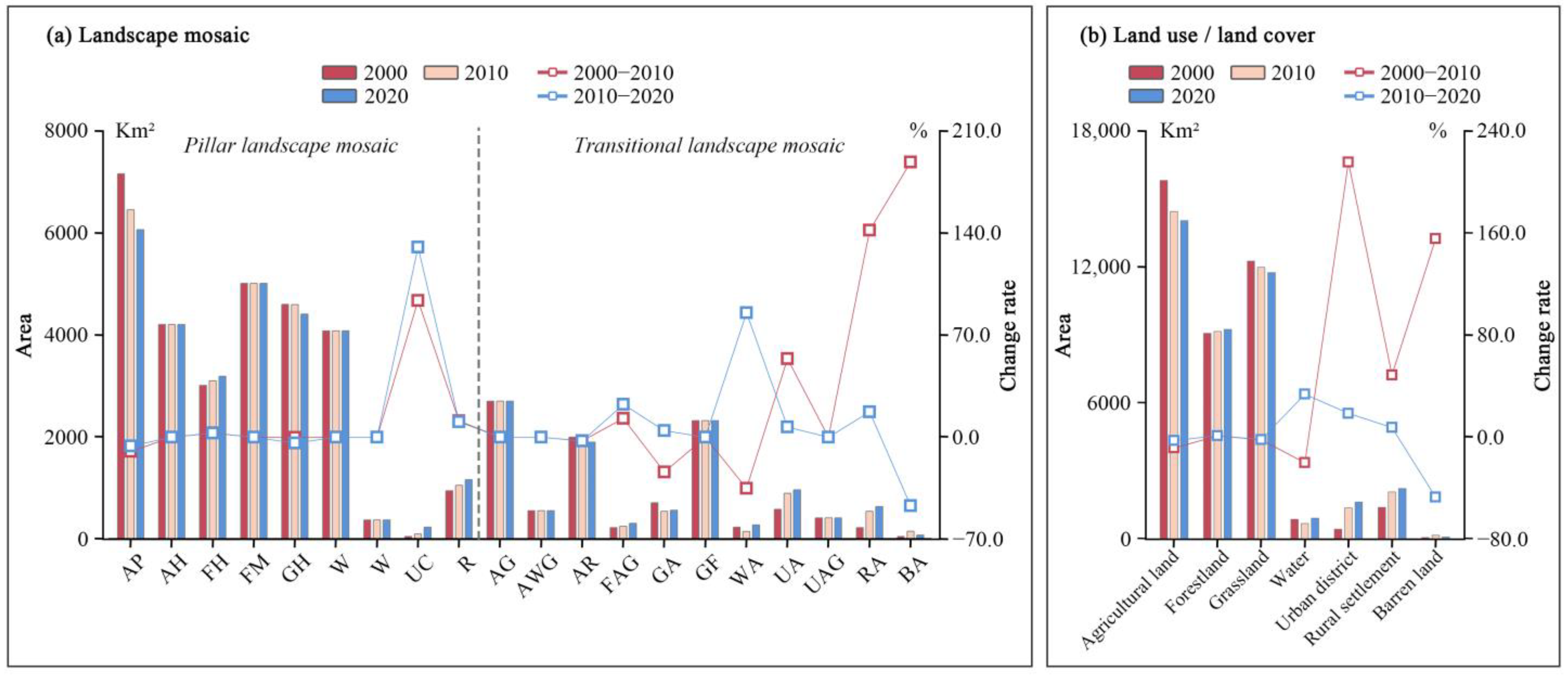
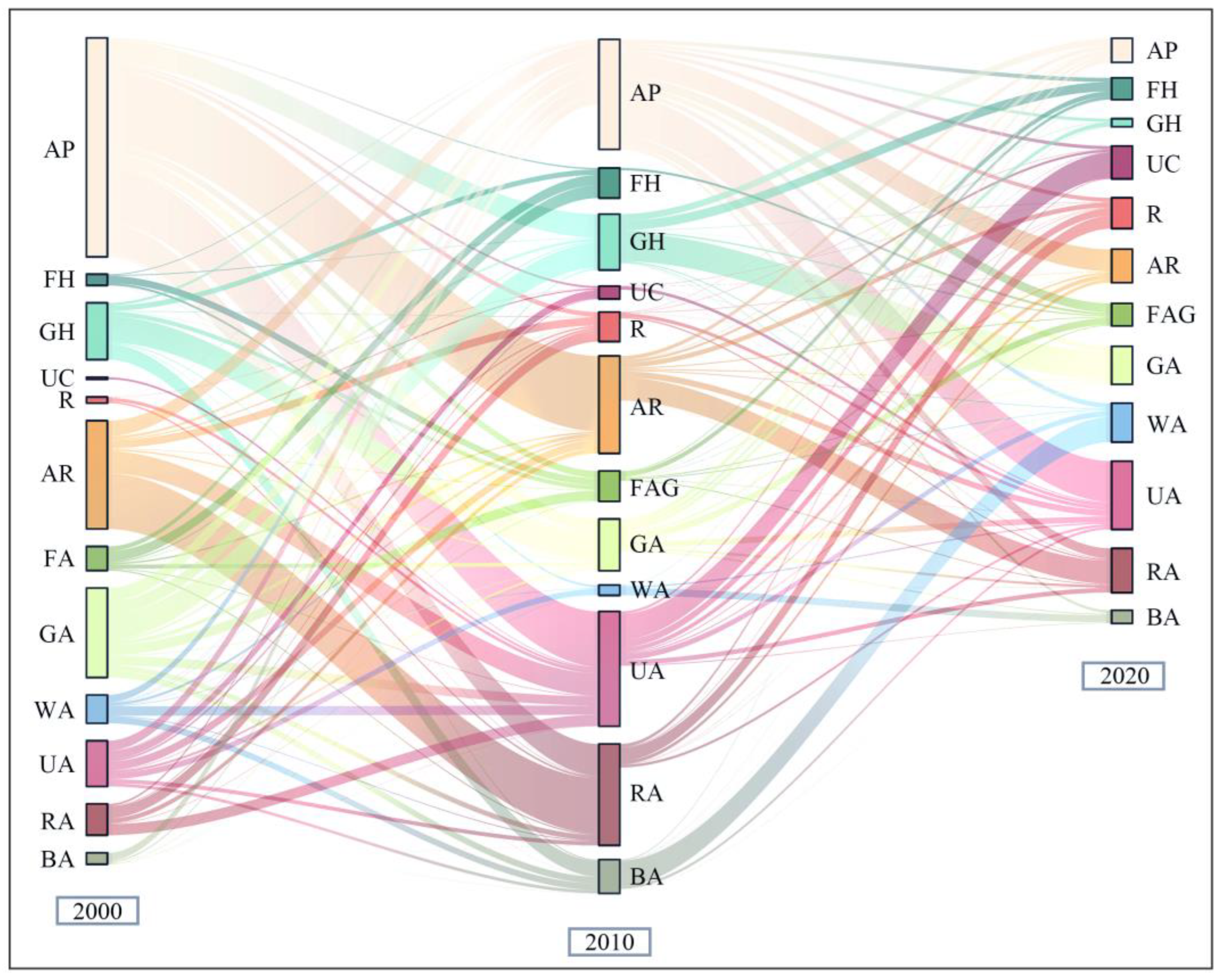
3.1.2. Area Change of Landscape Mosaic

Figure 4a illustrates the area proportions and change rates of land cover classification results in the study area from 2000 to 2020. It is evident that the PLM, primarily composed of farmland (AP and AH), forests (FM), and grasslands (GH), dominates the study area, collectively accounting for approximately 50% of the total area. The agricultural land in plain areas (AP) comprises approximately 18% of the total area, while the forests in mountainous regions (FM) account for roughly 13%. Additionally, the grasslands and agricultural lands in hillside areas (GH and AH) each represent about 11%. In contrast, TLM constitutes less than 30% of the total area, indicating that a single element predominantly characterizes most landscape mosaic types in the study area. Within the TLM category, the area proportions of the transitional zones between agricultural land and grassland, rural settlements (AG and AR), and between forests and grassland (GF) are more pronounced than those of other TLM types, each maintaining a stable area of around 6%, with a total area ranging between 2000 and 3000 km2. Analyzing the temporal evolution, the area and proportion of landscape patches in the study area experienced significant changes throughout the research period, which is a result of the rapid urbanization development in Hebei Province, China [5,86]. Notably, the overall change in landscape patches from 2000 to 2010 was slightly greater than that from 2010 to 2020. From 2000 to 2010, the total area of arable landscape in plains (AP) decreased from 7157.88 km2 to 6455.61 km2, reflecting a decline of 9.81%, marking the most substantial change in landscape mosaics during the study period. Conversely, the total area of barren–arable land transitional area (BA) increased from 54.00 km2 to 155.88 km2, representing a remarkable increase of 188.67%, the most significant landscape mosaic change event during the study period. Additionally, the dynamic changes in the transitional spaces between cultivated land, urban areas, and rural settlements (UC, UA, and RA) are significant.
For comparison, Figure 4b illustrates the changes in LULC from 2000 to 2020. The change patterns observed in LM and LULC classifications are largely consistent, suggesting that the LM classification results align well with the actual conditions. However, LM provides more detailed information regarding spatial evolution than LULC. Additionally, the spatial transformation analysis presented in Figure 5, Table A4 and A5 reveals that the transition areas between cultivated land, rural residential areas, grasslands, and urban built-up areas (AP, AR, GA, and UA) exhibit notably significant dynamic transformations. Within the LM framework, transitional spaces often require greater stability. Throughout the study period, the primary transformation phenomena observed include LM transitions from agricultural to rural (e.g., AP to AR), urban peripheral to bare soil (UA to BA), and rural to urban (AR to UC).

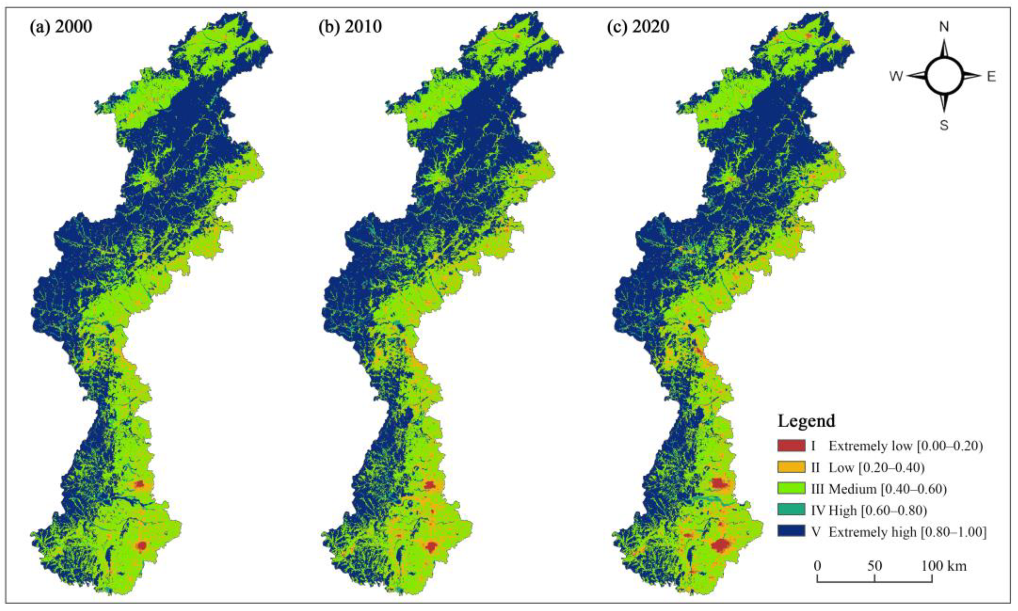
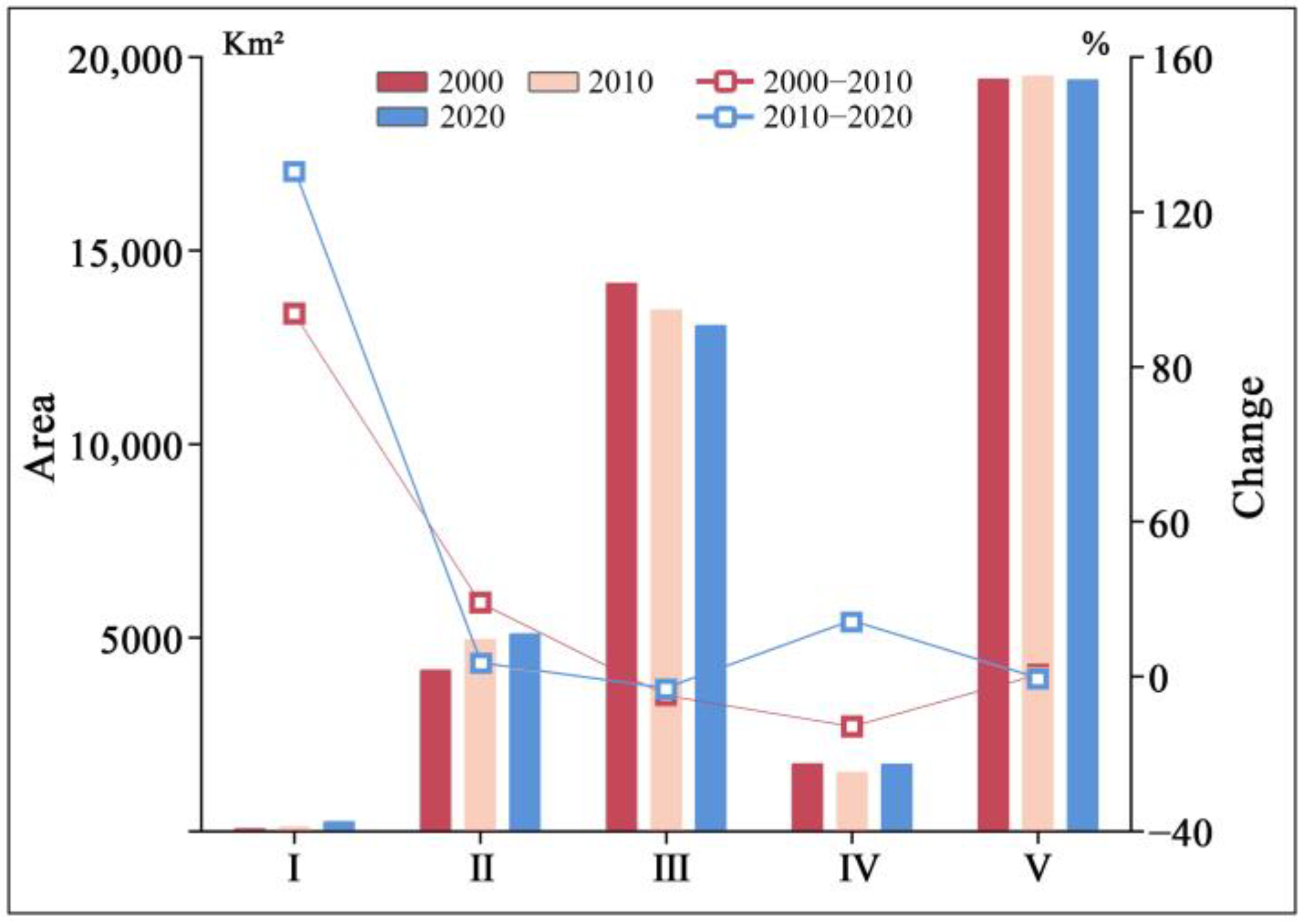
3.2. Spatiotemporal Pattern of Habitat Quality

In order to present the assessment results based on InVEST-HQ more clearly, HQ values were categorized into HQ levels ranging from I (extremely low) to V (extremely high). As illustrated in Figure 6 and Figure 7, the habitat quality index of the study area predominantly falls within Level V, representing approximately 50% of the total area. This level is primarily distributed across the northern and western mountainous regions, underscoring the significance of the study area for the ecological barrier function and ecosystem service value of the Beijing–Tianjin–Hebei urban agglomeration. The third-level habitat quality area ranks second, encompassing about 34% of the total area, and is situated in the transition zone between mountainous regions and plains, as well as in the northern basin area of the study area. The second-level habitat quality area accounts for roughly 11% of the total area and is located at the peripheries of urban centers in various cities and towns. Habitat areas classified as Level IV in quality are primarily found in valleys and foothills, comprising about 4% of the total area. In contrast, areas with Level I habitat quality represent the smallest proportion and are concentrated in the central urban area located in the southern part of the study area.
During the HQ evolution period, the area classified as Level III experienced a significant reduction in size, with the total area decreasing from 14,149.50 km2 to 13,060.10 km2 between 2000 and 2020. This represents a reduction rate of 7.85% from its initial state, marking it as the level with the largest decrease in the habitat quality area. Conversely, the habitat quality area of Level II has expanded considerably, increasing from 4154.49 km2 to 5089.86 km2, which corresponds to a growth rate of 21.96%. In comparison, the habitat quality area of Level V remains relatively stable overall. Although the habitat quality area of Level IV has seen a slight increase, it previously experienced a decrease of 12.93%, followed by an increase of 14.00%, contributing to the overall stability of the ecosystem. Based on the previously established habitat suitability of various LM habitats and the results of LM spatial transformation analysis, it is evident that the evolution of TLM is the primary driver behind changes in habitat quality areas across all levels. TLMs such as GA, RA, and UA play a crucial role in this process, underscoring their importance in biodiversity conservation and ecosystem restoration efforts.
Figure A1 and Figure A2 and Table A6 and Table A7 present the parameters and results of the InVEST-HQ model evaluation based on LULC. Statistically, the analysis based on LULC shows a larger area of Level I and Level V HQ zones, while the areas of Level II and Level IV HQ zones are relatively smaller, and the area of Level III habitat quality zones is quite similar. For instance, in 2020, the areas of Level I and Level V HQ zones based on LULC assessment were 830.29 km2 and 21,732.00 km2, respectively, which are larger by 595.39 km2 (253.47%) and 2329.43 km2 (12.01%) compared to the LM-based assessment results. Conversely, the areas of Level II and Level IV HQ zones were 3121.44 km2 and 182.17 km2, respectively, which are smaller by 1968.40 km2 (38.67%) and 1538.40 km2 (89.41%) than the LM-based assessment results. In conjunction with the spatial visualization results (Figure 8), in most areas, the LM-based assessment results show little difference from those based on LULC (−0.10 to 0.10). In areas where the differences are more pronounced, the LM-based assessment results have higher values and are more concentrated in urban fringe areas, while the areas with higher LULC assessment results are scattered in hillside regions. Overall, the HQ assessment results based on the data from the two classification systems largely address the theoretical content and academic viewpoints presented in the earlier sections of this paper [27,28,29,30]. In conjunction with the spatial distribution analysis of LM classification results, the impact of TLMs on HQ evaluation results manifests primarily in two directions: (1) The emergence of TLMs such as AG, FAG, and GA indicates that areas with concentrated forest- and grassland do not necessarily correspond to a higher habitat quality index. (2) The presence of TLMs such as UA, RA, and UAG suggests that areas with concentrated urban built environments may exhibit a higher habitat quality index value compared to areas within the urban core.

3.3. Impacts of Landscape Mosaic Pattern on Habitat Quality Based on OLS Model

There exists a notable interaction between LULC structure and HQ [87,88]. We employed OLS model to quantify the correlation between LM patterns and HQ, as well as to compare the impacts of LM and LULC patterns on HQ. Table 6 presents the results of variance analysis for the OLS models across different years. Overall, a significant interactive relationship exists between the four pattern indices and HQ (p < 0.01, VIF < 7.50). FRAC_MN exhibits the strongest correlation with the SPLIT, with correlation coefficients for all instances exceeding 0.70 throughout the study period, indicating a positive driving effect. Conversely, SHDI demonstrates a negative driving relationship, with correlation coefficients around −0.450, suggesting a notable influence. Additionally, the CONTAG index and HQ value exhibit a positive relationship; however, their interaction strength is less than that of FRAC_MN and SPLIT.
From 2000 to 2020, the correlation between FRAC_MN and SPLIT patterns with HQ exhibited a dynamic process characterized by an initial strengthening followed by a subsequent weakening. Overall, the correlation remained robust. In contrast, the correlations between CONTAG and SHDI patterns with HQ consistently increased throughout the study period, indicating that the significant changes in land management dynamics substantially altered the original pattern state of the study area. Factors such as complex patch edges (FRAC_MN), continuity between patches (SPLIT, CONTAG), and diversity of patch types (SHDI) all influence the HQ index. This further reinforces the previous conclusion that targeted land management necessitates a greater emphasis on biodiversity conservation.

3.4. Impacts of Landscape Mosaic Pattern on Habitat Quality Based on GWR Model

The evaluation results of the OLS model can only represent the correlation in a mathematical context. To further elucidate the spatial differences in the correlation between the LM pattern index and HQ, we selected the Bi-Square spatial weight model in the SAM4.0 software and conducted a GWR model analysis based on this. Figure 9 presents the GWR correlation results between the FRAC_MN, SPLIT, CONTAG, and SHDI indices and HQ in the study area from 2000 to 2020. Regarding spatial quantification, the same LM pattern index exhibits varying, and at times opposing, driving effects across different regions. Notably, the FRAC_MN index demonstrates a strong positive driving effect (β > 3.0) in the transition zone between urban and rural built-up areas and hillsides; however, this area is gradually diminishing, with some regions in the southern part of the study area even shifting to a negative driving direction. This indicates that complex patch edges often signify a greater diversity of landscape elements and TLM components in areas with high urbanization intensity, which naturally become valuable biological habitat resources. Nonetheless, as urban and rural construction land expands, the differences in complexity among various types of LM patches have diminished, and their influence on HQ is not as pronounced as it was during the initial stages of the study. The spatial relationship between the SPLIT and CONTAG indices and HQ is analogous to that of the FRAC_MN index; however, the overall driving force is diminished. In the LM patch pattern, edge complexity emerges as a more critical factor than fragmentation. The absolute correlation value between the SHDI and HQ is lower than that of the other three pattern indices, indicating a relatively straightforward spatial variation. Specifically, diverse LM types are more likely to signify higher-quality biological habitats in the hillsides. Notably, during the study period, the area characterized by a high SHDI (β > 0.50) has contracted, suggesting that urban development has negatively impacted the biodiversity support service capacity of urban–rural fringes and hillside zones.

4. Discussion

4.1. LM Classification Method Integrating PCA-SOM-ED Composite Model

To achieve systematic and efficient LM classification, various methods—such as LPT, MLT, LUs, and TPM—were reviewed and compared based on extensive literature analysis [34,35,36,37,38,39,40,41,42,89]. Our research primarily builds upon the methodologies proposed by Vizzari et al. [35], while also incorporating modifications to align with our objectives. Specifically, we have integrated models such as PCA, SOM, and ED to develop a comprehensive classification system for LM. This approach introduces several modifications: (1) Natural and socio-economic factors, including elevation, slope, GDP, and VIIRS, were incorporated into the LM classification process, creating a more comprehensive base factor system. (2) The ISODATA model should be replaced by the SOM model, which provides a more convenient representation of the LM across multiple time periods in accordance with unified standards. (3) ED was used to validate classification results and enhanced the accuracy of the LM classification framework. By calculating the intra-cluster sum of squares for SOM classification and mapping it to LM classification, the study achieved a scenario of “minimal intra-cluster differences and maximal inter-cluster differences on principal components (PCs)”. In the empirical analysis of LM classification, seven LULC types in the Taihang Mountains in Hebei Province were classified into nine types of PLMs and eleven types of TLMs. These numbers exceed previous classifications for the same region (five PLMs and six TLMs) [90] and those in Vizzari et al.’s [35] study in France (five PLMs and eight TLMs). This increase can be attributed to the combined effects of the changes in the aforementioned three approaches.
This study enhances the logical framework of LM classification by integrating multiple factors such as natural environment, vegetation type, urban–rural construction, and socio-economic attributes. The method is applicable across diverse spatiotemporal scales and landscape types. However, several limitations remain: (1) Although the optimal LM classification scenario was derived using Euclidean distance, it remains confined to the realm of mathematical statistics. Further research is required to ascertain whether the classification results sufficiently reflect the structure of the complex ecosystem within the study area. Additionally, the processing of LULC data in this paper is relatively cumbersome; leveraging the powerful computational capabilities of ESRI ArcGIS may allow for significant simplification of this process. (2) Various classification methods, such as landscape features, ecological units, and landscape units, share similarities with the classification of landscape mosaics. Furthermore, there are numerous classification algorithms that can be further explored, including supervised nearest neighbor, machine learning, and deep learning. (3) We conducted LM classification based on 12 factors. The resolution of the relevant factor data, the uniformity of time coverage, and the sensitivity of the LM classification results present scientific issues that warrant further exploration in the future. At the same time, we conducted LM classification using primary LULC types such as forests and grasslands. In contrast, a secondary LULC classification system can significantly enhance the expression of local plant mosaic characteristics in the study area during LM classification. (4) Referencing existing research findings [35], we utilized a 300 × 300 m grid cell to aggregate all foundational data for conducting land cover classification. However, the rationale behind this grid cell size still requires comparative discussion.

4.2. InVEST-HQ Model Assessment Using LM Instead of LULC

This study introduces a significant innovation in HQ assessment by employing LM classifications instead of the commonly used LULC data in the InVEST-HQ model. The primary aim was to bridge the gap between the model’s parameter settings and the ecological realities observed in field investigations regarding differences in biological habitats. From a landscape ecology perspective, the structural differences between LULC patch edges and interiors introduce variability in ecosystems’ capacity to support biodiversity [22]. As Ostermann highlighted, transitional spaces are among the most biodiverse and critical habitats for supporting endangered species [91]. This perspective has been expressed in studies of typical cases such as the treeline ecotone in the European mountains, the Andes mountains in the tropics, and the ecological transition zones of the tropical rainforests in Cameroon [92,93,94].
By using LM as the basic habitat type, this study accounted for spatial heterogeneity and ecological nuances often overlooked in LULC-based assessments. Specific habitat suitability parameters were established for various TLMs and PLMs. The results showed significant differences compared to LULC-based assessments [95]. LM-based assessments more accurately captured the complex ecosystem structures of the study area, demonstrating potential for expansion into other ecosystem service evaluations, such as soil and water conservation or water source protection [96,97]. Despite its innovations, the study faced several challenges. The fundamental parameters have a complex impact on the evaluation results of the InVEST-HQ model. This study presents a novel setting for the threats parameter and the sensitivity of different LM to threatening factors. The habitat suitability parameters for TLMs were informed by extensive field investigations but lacked comprehensive measured data and systematic research on target species [98,99]. While the theoretical basis for LM’s application in HQ assessment is robust, its practical validation relies on more accurate baseline data and expanded studies across different scales and geographic units.

4.3. Targeted Development Suggestions

Based on the results, the following strategies are proposed to protect and enhance biodiversity in the Taihang Mountains of Hebei Province.
The statistical analysis of LM spatial transformation and HQ classification indicates that, during the study period, the V-level habitat quality areas, predominantly characterized by FM, FH, and GM, remained largely stable. This stability aligns with the ecological positioning of the region within the Hebei Province Land and Space Planning framework. However, it is crucial to closely monitor the changes in Level IV and Level III-habitat quality areas. The Level IV areas, primarily dominated by GA and WA, exhibited minor fluctuations in size throughout the study period. In light of this, relevant authorities should enhance the ecological protection red line system to safeguard key ecological sources and biological habitats from human disturbance and degradation. Although the Level I habitat quality area contributes minimally overall, it plays a significant role in the daily lives of residents. Therefore, within urban built-up areas, it is essential to underscore the importance of ecological networks. This can be achieved by leveraging urban arterial roads, rivers, and other infrastructures to develop large-scale green initiatives, particularly by linking TLMs such as forest–grassland, forest–cropland, and grassland–cropland, treating them as critical corridor structures within the ecological network and enhancing their connectivity.
The correlation analysis between LM patterns and HQ indicates that the complexity of LM patch edge structures and the diversity of LM types are the primary influencing factors. It is essential to propose targeted strategies based on these differential research findings. In the hillside zone, TLM types such as FA, GA, and RA serve as core carriers of biological habitats. The standardization of human agricultural activities in this area will significantly impact biodiversity. Therefore, it is recommended to increase green spaces, such as farmland shelterbelts and ecological buffer forests. In the expansive plains, the study area necessitates a greater diversity of LM types to enhance the survival opportunities of local organisms, such as the establishment of agricultural shelterbelts and ecological green belts along irrigation channels. During future urban construction and expansion, it is advisable to adopt a ‘jumping’ rather than a ‘spreading’ construction model to minimize the connectivity of impermeable surfaces [100].

5. Conclusions

As essential components of terrestrial ecosystems, mountainous areas are characterized by rich biodiversity and high levels of ecosystem productivity. However, these regions are also fragile and particularly sensitive to climate change and LULC changes. In this context, a substantial body of academic work has been conducted to assess and analyze biodiversity in mountain regions using the InVEST-HQ model. Nevertheless, it has been observed that the evaluation results from the InVEST-HQ model are overly reliant on LULC data, especially in mountainous areas with significant landscape heterogeneity. Our study addresses these research gaps by conducting empirical research in the Taihang mountainous area of Hebei Province, China. Initially, spatial data encompassing natural conditions, vegetation resources, urban and rural development, and the social economy of the study area were collected to establish a comprehensive database. Subsequently, a PCA-SOM-ED composite model was employed to classify the landscape mosaic patterns within the study area, thereby elucidating the characteristics and dynamics of landscape heterogeneity. Our findings indicate the following: (1) Utilizing LM classification results instead of LULC data as the foundation for evaluating the InVEST-HQ model can facilitate the integration of diverse research findings from numerous field surveys into the InVEST-HQ model. (2) The influence of LM patterns on HQ is complex; variations in landform conditions and the urban–rural construction environment significantly affect the correlation between these two factors. (3) Regarding biodiversity protection and enhancement within the study area, we observed that transitional landscape mosaics—such as the transition spaces between forest-cultivated land and grassland-cultivated land—exhibited reduced dynamism during the study period, necessitating increased attention from relevant authorities. The resulting classification of landscape mosaics was integrated into the InVEST-HQ model for analysis, which alleviated the limitations of LULC data and yielded more precise assessments of habitat quality. This paper takes mountainous areas as an example to explore the impact of composite landscape mosaics on biodiversity. This approach can serve as a future direction for this research, considering its applicability to other mountainous regions, its feasibility for studies on supporting watersheds and urban agglomerations, and the differences in various social governance contexts.

Author Contributions

Conceptualization, J.F. and Y.H.; methodology, J.F.; software, J.F. and P.H.; validation, M.Y., K.D., and Y.Z.; formal analysis, J.H.; investigation, J.F., P.H., and J.H.; resources, J.F. and Y.H.; data curation, J.F. and P.H.; writing—original draft preparation, J.F. and P.H.; writing—review and editing, J.F., J.H., and P.H.; visualization, M.Y.; supervision, J.F., P.H., and M.Y.; project administration, J.F.; funding acquisition, J.F. and Y.H. All authors have read and agreed to the published version of the manuscript.

Funding

This research was funded by the Research Project of Basic Scientific Research Business Expenses of Universities in Hebei Province, China (1002257), and the Science and Technology Plan Carry-over Project in Hebei Province, China, specifically focusing on the Modern Forestry Seed Industry Science and Technology Innovation Team (21326301D).

Institutional Review Board Statement

Not applicable.

Informed Consent Statement

Not applicable.

Data Availability Statement

The data presented in this study are available on request from the corresponding author.

Conflicts of Interest

The authors declare no conflicts of interest.

Appendix A

Table A1. LM typologies (PLM: pillar landscape mosaic; TLM: transitional landscape mosaic), codes, and related descriptions.
TypeAbbreviationsLM NameGeneral Description
PLMAPArable landscape in plainsThe landscape exhibits a continuous high-density texture of farmland, interspersed with a limited number of rural residential areas and agricultural facilities.
AHArable landscape in hillsidesThe composition of LULC is identical to that of AP. The primary distinction lies in its geographical location, situated on a hillside with a specific slope.
FHForest landscape in hillsidesForest landscape predominantly consists of trees and shrubs, primarily located in hilly regions. A limited number of these landscapes can be found near urban areas, where they depend on green spaces such as forest parks and nature reserves.
FMForest landscape in deep mountain areasForest landscape situated in a mountainous region characterized by steeper terrain and predominantly retains a natural state.
GHGrass landscape in hillsidesGrass landscape encompasses both natural and artificial grassland features. It includes a limited extent of cultivated land, woodlands, and rural settlements, all located within a hillside zone.
GMGrass landscape in mountain areasGrass landscape situated in a mountainous region characterized by steeper terrain and predominantly retains a natural state.
WWater landscapeThe relatively concentrated rivers, lakes, and reservoirs represent valuable surface water resources within the study area.
UCUrban core landscapeUrban landscapes characterized by a continuous urban fabric demonstrate the highest levels of population density within the study area, alongside average GDP and average light DN values.
RRural settlement landscapeIn urban and rural built-up areas, where impervious surfaces and farmland intermingle, population density, average GDP, and nighttime light intensity are relatively low.
TLMAGArable land–grassland transitional areaLandscape characterized by farmland and grassland elements, typically situated at the peripheries of rural settlements.
AWGArable land–water–grassland transitional areaLandscape characterized by the predominance of farmland, water bodies, and grassland, situated on the rural periphery of the valley.
ARArable land–rural settlement transitional areaSituated on the periphery of cities and villages, the area features relatively clustered rural residential zones at its core, creating a landscape characterized by the intermingling of farmland and rural housing.
FAGForest–arable land–grass transitional areaLandscape characterized by a combination of cultivated land, woodland, and grassland. This type of landscape occurs only under specific terrain conditions.
GAGrass–arable land transitional areaThe landscape texture is consistent with that of AG; however, the primary distinguishing factor is the shift in the dominant element type from farmland to grassland.
GFGrass–forestland transitional areaLandscape space transitions between woodland and grassland, typically found in steeper mountainous terrain.
WAWater–arable land transitional areaLandscape situated on both banks of the river, where farmland is relatively concentrated. Although it occupies a small area within the study region, it is widely distributed.
UAUrban–arable land transitional areaLandscape adjacent to urban built-up regions, which reflects the spatial characteristics associated with the periphery of urban development.
UAGUrban–arable–grassland transitional areaLandscape exhibits a similar formation mechanism to that of UA. A significant distinction lies in the heightened presence of industrial buildings, which act as impermeable surfaces within the landscape.
RARural–arable land transitional areaThis region is characterized by a transitional landscape comprising rural settlements and agricultural land. It generally commences from location R and extends outward in a “finger-like” configuration along transportation routes or waterways. The population and socio-economic conditions of this area are surpassed only by those of location R.
BABarren–arable land transitional areaBare soil and wasteland constitute the primary landscape features of this spatial type, with a limited presence of farmland landscapes in the region.
Table A2. Landscape mosaic codes and areas in 2000 with the average percentages of LULC macro classes for each landscape type; gray cells include percentages, summing to at least 75%, used for landscape mosaic coding.
Landscape Mosaic TypeArea
(km2)
Area
(%)
X1X2X3X4X5X6X7X8X9X10X11X12
AP7157.880.18177.932.250.3974.790.341.800.070.761.850.164.4756.96
AH4205.250.11593.166.150.2672.792.114.030.040.010.750.011.272.43
FH3016.980.08741.4320.830.2410.6383.435.570.020.060.050.010.481.80
FM5014.530.131210.1628.710.010.3997.212.370.010.010.010.010.200.87
GH4601.250.12385.8115.220.324.720.8493.900.020.050.150.011.184.90
GM4081.590.10832.3624.180.042.293.5194.130.010.010.020.010.520.49
W379.800.01276.581.9485.597.730.523.732.070.130.230.022.757.88
UC52.650.0188.462.420.0110.730.010.240.0187.751.2820.90105.807928.93
R950.580.02196.182.290.2331.290.501.890.040.2365.810.185.0767.17
AG2706.480.07546.4712.940.2649.392.2447.710.010.040.350.011.133.88
AWG558.180.01378.047.8434.9639.404.4319.640.630.050.880.011.965.61
AR2001.510.05243.703.490.4771.501.274.800.030.4621.470.234.7481.96
FAG225.450.01776.4016.332.8128.4738.9025.062.730.461.580.061.1626.44
GA715.770.02445.9711.251.7229.193.1563.140.251.760.790.162.0345.88
GF2323.710.061037.7525.330.051.8042.1455.980.010.010.010.010.331.10
WA234.000.01174.871.7271.2224.961.341.350.190.250.990.244.4681.87
UA586.800.01163.702.5310.1543.010.372.4104042.301.362.5017.761048.30
UAG516.430.01391.6210.311.6942.529.9031.250.0812.472.090.143.2775.81
RA225.090.01131.491.960.5845.710.431.060.050.1951.980.7010.10266.60
BA54.000.01756.003.840.6725.831.674.8864.980.211.780.163.7057.68
Table A3. Landscape mosaic codes and areas in 2010 with the average percentages of LULC macro classes for each landscape type; gray cells include percentages, summing to at least 75%, used for landscape mosaic coding.
Landscape Mosaic TypeArea
(km2)
Area
(%)
X1X2X3X4X5X6X7X8X9X10X11X12
AP6455.610.16177.982.140.2692.910.331.430.023.191.870.343.86287.16
AH4205.250.11593.166.150.1792.912.153.920.010.130.700.011.177.80
FH3103.740.08745.3920.680.1210.0983.525.440.030.430.360.010.437.70
FM5014.530.131210.1628.710.010.3797.182.370.010.050.030.010.141.83
GH4597.650.12393.4515.050.304.170.7993.290.020.780.650.021.0616.32
GM4091.590.10832.3624.180.022.263.5793.990.010.080.070.010.416.45
W379.800.01276.581.9478.718.111.284.496.011.170.230.052.9456.39
UC101.970.01137.502.320.696.650.010.130.0192.240.2815.8474.2011,534.82
R1057.140.03196.282.370.0814.530.240.960.010.8693.320.488.75332.78
AG2706.480.07546.4712.940.2248.912.2447.680.010.230.720.011.0811.94
AWG556.180.01378.047.8433.5239.174.2418.351.791.371.560.062.3037.81
AR1952.010.05256.523.590.3259.731.093.820.062.7432.230.404.93305.20
FAG254.610.01746.6717.221.2120.5544.4323.260.337.632.580.130.9383.49
GA544.320.01450.0312.560.9624.124.5259.120.508.891.900.322.30209.67
GF2323.710.061037.7525.330.031.7542.1555.860.010.130.070.010.262.58
WA152.100.01176.222.0372.8120.520.853.210.012.030.580.354.17457.52
UA902.340.02164.642.623.6726.160.201.101.0167.160.704.6119.133429.76
UAG416.430.01391.6210.311.2727.237.1520.520.1742.411.260.253.98215.36
RA544.590.01165.642.450.6840.030.321.900.061.8755.140.848.33671.94
BA155.880.01115.012.020.0919.300.501.9775.710.991.140.162.72105.92
Table A4. Landscape mosaic matrix from 2000 to 2010 (km2).
APFHGHUCRARFAGGAWAUARABA
AP——6.93108.1810.1722.14343.6233.2160.3910.89251.82145.085.76
FH3.69——3.690.000.000.0932.2210.440.720.000.270.00
GH12.0624.84——0.002.790.9920.52118.890.544.592.5271.37
UC0.090.000.09——0.090.000.000.180.009.90.270.00
R1.170.000.001.71——0.810.090.450.0016.118.190.27
AR70.200.0912.516.3936.99——2.978.281.17101.34253.440.72
FAG21.4246.175.940.091.447.38——18.270.543.515.590.09
GA61.5659.67113.850.188.4617.0146.35——3.3342.1224.5730.78
WA33.660.001.350.361.4411.610.902.88——42.484.4130.33
UA45.810.092.5237.089.9038.342.8811.2527.81——18.4514.31
RA9.900.000.363.9652.1122.050.273.060.6350.67——0.54
BA36.360.097.020.000.002.700.092.341.891.440.36——
Note: The vertical coordinate label represents the LMs that underwent type transformation from 2000 to 2010, while the horizontal coordinate label denotes the LMs that were transformed during the same period.
Table A5. Landscape mosaic matrix from 2010 to 2020 (km2).
APFHGHUCRARFAGGAWAUARABA
AP——18.4514.2215.4818.27101.0742.7522.0522.41186.3946.6213.59
FH0.18——0.000.000.000.0010.620.000.180.000.000.00
GH31.1442.66——0.001.980.636.84130.680.095.313.151.44
UC0.180.000.00——1.080.540.000.000.4514.400.360.09
R1.350.000.091.71——2.250.000.720.0916.386.660.00
AR17.820.092.1610.822.41——5.045.674.9528.44105.660.63
FAG4.0522.680.000.271.441.35——4.864.591.714.680.00
GA22.6814.4918.541.442.348.9132.40——2.3427.5411.706.12
WA2.430.000.000.360.540.630.181.17——7.291.1733.84
UA11.700.721.71116.8233.7520.434.865.7626.01——21.784.59
RA14.850.000.543.1558.8615.930.091.081.0811.88——0.00
BA3.420.000.090.000.090.990.180.63115.2912.330.63——
Note: The vertical coordinate label represents the LMs that underwent type transformation from 2010 to 2020, while the horizontal coordinate label denotes the LMs that were transformed during the same period.
Table A6. Information on threat parameter.
Threat FactorMaximum Distance (km)Weight (0.1)Decay
Agricultural land1.00.50Exponential distance-decay
Urban district6.00.80Linear distance-decay
Rural settlement1.80.70Exponential distance-decay
Expressway and railroad networks4.00.50Exponential distance-decay
Main road network in urban district2.00.30Exponential distance-decay
Table A7. The sensitivity of different landscapes to threatening factors.
Land Use/Land Cover TypeHabitatAgricultural LandUrban DistrictRural SettlementExpressway and Railroad NetworksMain Road Network in Urban District
Agricultural land0.500.000.700.350.850.70
Forestland1.000.550.900.750.900.75
Grassland0.900.700.850.800.900.75
Water0.850.750.950.800.800.80
Urban district0.000.000.000.000.600.45
Rural settlement0.350.000.000.000.750.55
Barren land0.300.000.000.000.800.60
Figure A1. The spatial distribution of the habitat quality district based on LULC.
Sustainability 17 05503 g0a1
Figure A2. The area and change rate of the habitat quality district based on LULC.
Sustainability 17 05503 g0a2

References

  1. Yang, J.; Xie, B.P.; Tao, W.Q.; Zhang, D.G. Ecosystem Services Assessment, Trade-Off, and Bundles in the Yellow River Basin, China. Diversity 2021, 13, 308. [Google Scholar] [CrossRef]
  2. Ding, Q.L.; Chen, Y.; Bu, L.Y.; Ye, Y.M. Multi-scenario analysis of habitat quality in the Yellow River delta by coupling FLUS with InVEST model. Int. J. Environ. Res. Public Health 2021, 18, 2389. [Google Scholar] [CrossRef]
  3. Xie, B.; Zhang, M. Spatio-Temporal Evolution and Friving Forces of Habitat Quality in Guizhou Province. Sci. Rep. 2023, 13, 6908. [Google Scholar]
  4. Zhu, C.M.; Zhang, X.L.; Zhou, M.M.; He, S.; Gan, M.Y.; Yang, L.X.; Wang, K. Impacts of urbanization and landscape pattern on habitat quality using OLS and GWR models in Hangzhou, China. Ecol. Indic. 2020, 117, 106654. [Google Scholar] [CrossRef]
  5. Yang, Y.Y. Evolution of habitat quality and association with land-use changes in mountainous areas: A case study of the Taihang Mountains in Hebei Province, China. Ecol. Indic. 2021, 129, 107967. [Google Scholar] [CrossRef]
  6. Wu, J.Y.; Luo, J.G.; Zhang, H.; Qin, S.; Yu, M.J. Projections of land use change and habitat quality assessment by coupling climate change and development patterns. Sci. Total Environ. 2022, 847, 157491. [Google Scholar] [CrossRef] [PubMed]
  7. Zhang, N.N.; Wu, X.F. Influence of urban land use compact change on riparian habitat: A case study of Wuhan section of Hanjiang river small watershed. Chin. Landsc. Archit. 2021, 37, 87–91. [Google Scholar]
  8. Sherrouse, B.C.; Semmens, D.J.; Clement, J.M. An application of Social Values for Ecosystem Services (SolVES) to three national forests in Colorado and Wyoming. Ecol. Indic. 2014, 36, 68–79. [Google Scholar] [CrossRef]
  9. Bagstad, K.J.; Semmens, D.; Villa, F.; Johnson, G.W. Quantifying and valuing ecosystem services: An application of ARIES to the San Pedro River basin, USA. In Handbook on the Economics of Ecosystem Services and Biodiversity; Edward Elgar Publishing: Cheltenham, UK, 2014; p. 169. [Google Scholar]
  10. Boumans, R.; Roman, J.; Altman, I.; Kaufman, L. The Multiscale Integrated Model of Ecosystem Services (MIMES): Simulating the interactions of coupled human and natural systems. Ecosyst. Serv. 2015, 12, 30–41. [Google Scholar] [CrossRef]
  11. Yan, S.J.; Wang, X.; Cai, Y.P.; Li, C.H.; Yang, Z.F.; Yi, Y.J. Investigation of the spatio-temporal dynamics in landscape variations in a shallow lake based on a new Tendency-Pattern-Service conceptual framework. J. Clean. Prod. 2017, 161, 1074–1084. [Google Scholar] [CrossRef]
  12. Sun, X.Y.; Jiang, Z.; Liu, F.; Zhang, D.Z. Monitoring spatio-temporal dynamics of habitat quality in Nansihu Lake basin, eastern China, from 1980 to 2015. Ecol. Indic. 2019, 102, 716–723. [Google Scholar] [CrossRef]
  13. Ye, H.; Song, Y.Y.; Xue, D.Q. Multi-Scenario Simulation of Land Use and Habitat Quality in the Guanzhong Plain Urban Agglomeration, China. Int. J. Environ. Res. Public Health 2022, 19, 8703. [Google Scholar] [CrossRef]
  14. Tang, F.; Fu, M.C.; Wang, L.; Zhang, P.T. Land-use change in Changli County, China: Predicting its spatio-temporal evolution in habitat quality. Ecol. Indic. 2020, 117, 106719. [Google Scholar] [CrossRef]
  15. Chen, C.Y.; Liu, J.; Bi, L.L. Spatial and temporal changes of habitat quality and its influential factors in China based on the InVEST model. Forests 2023, 14, 374. [Google Scholar] [CrossRef]
  16. Chen, W.D.; Wang, R.; Liu, X.H.; Lin, T.; Hao, Z.; Zhang, Y.K.; Zheng, Y. The Interrelationships and Driving Factors of Ecosystem Service Functions in the Tianshan Mountains. Forests 2024, 15, 1678. [Google Scholar] [CrossRef]
  17. Wu, L.L.; Sun, C.G.; Fan, F.L. Estimating the characteristic spatiotemporal variation in habitat quality using the invest model—A case study from Guangdong–Hong Kong–Macao Greater Bay Area. Remote Sens. 2021, 13, 1008. [Google Scholar] [CrossRef]
  18. Yang, J.; Xie, B.P.; Zhang, D.G. Spatial-Temporal Evolution of Habitat Quality and Its Influencing Factros in the Yellow River Basin based on InVEST Model and GeoDetector. J. Desert Res. 2021, 41, 12–22. [Google Scholar]
  19. Zhang, X.; Liao, L.Y.; Xu, Z.D.; Zhang, J.Y.; Chi, M.W.; Lan, S.R.; Gan, Q.C. Interactive effects on habitat quality using InVEST and GeoDetector models in Wenzhou, China. Land 2022, 11, 630. [Google Scholar] [CrossRef]
  20. Turner, M.G. Landscape Ecology: The Effect of Pattern on Process. Annu. Rev. Ecol. Syst. 1989, 20, 171–197. [Google Scholar] [CrossRef]
  21. Singh, J.S.; Roy, P.S.; Murthy, M.S.R.; Jha, C.S. Application of Landscape Ecology and Remote Sensing for Assessment, Monitoring and Conservation of Biodiversity. J. Indian Soc. Remote Sens. 2010, 38, 365–385. [Google Scholar] [CrossRef]
  22. Forman, R.T.T.; Godron, M. Landscape Ecology; John Wiley and Sons: New York, NY, USA, 1986; pp. 10–30. [Google Scholar]
  23. Wang, R.S.; Li, F.; Hu, D.; Larry Li, B. Understanding Eco-complexity: Social-Economic-Natural Complex Ecosystem Approach. Ecol. Complex. 2011, 8, 15–29. [Google Scholar] [CrossRef]
  24. He, C.Y.; Zhang, J.X.; Liu, Z.F.; Huang, Q.X. Characteristics and progress of land use/cover change research during 1990–2018. J. Geogr. Sci. 2022, 32, 537–559. [Google Scholar] [CrossRef]
  25. Naveh, Z. Some Remarks on Recent Developments in Landscape Ecology as a Transdisciplinary Ecological and Geographical Science. Landsc. Ecol. 1991, 5, 65–73. [Google Scholar] [CrossRef]
  26. Liu, L.Y.; Bian, Z.Y.; Ding, S.Y. Effects of landscape spatial heterogeneity on the generation and provision of ecosystem services. Acta Ecol. Sin. 2018, 38, 6412–6421. [Google Scholar]
  27. Bian, Z.X.; Wang, C.Q.; Liu, Y.; Sun, Z.Q.; Wang, S.; Liu, S.; Zhu, S.; Yu, M. Ecological Network Characteristics of the Functional Group of Epigaeic Arthropod in Arable Land with Different Field Margin Types. Chin. J. Eco-Agric. 2022, 9, 1381–1392. [Google Scholar]
  28. Hou, J.H.; Gao, B.H.; Dong, J.X.; Gao, L.J.; Liu, Y.H.; Li, L.H. Community Diversity of Arthropod in Forest-steppe Ecotone in southeast Edge of Inner Mongolia Tableland. Scientia 2008, 3, 94–101. [Google Scholar]
  29. Li, Y.; Wang, D.M.; Xin, Z.B.; Wang, J.; Ren, Y.; Li, Q.S. Plant Diversity and Soil Characteristics of Different Inundation Zones in An Aquaticterrestrial Ecotone, Li River. Acta Ecol. Sin. 2015, 35, 5121–5130. [Google Scholar]
  30. Mao, Q.Z.; Ma, K.M.; Wu, J.G.; Tang, R.L.; Zhang, Y.X.; Luo, S.H.; Bao, L.; Cai, X.H. An Overview of Advances in Distributional Pattern of Urban Biodiversity. Acta Ecol. Sin. 2012, 33, 1051–1064. [Google Scholar]
  31. Lin, S.T.; Xie, D.B.; Liu, Y.L.; Chen, W.B. Study on the Relationship between Landscape Pattern and Regional Biodiversity. Ecol. Environ. Sci. 2017, 26, 1681–1688. [Google Scholar]
  32. Dramstad, W.E.; Olson, J.D.; Forman, R.T.T. Landscape Ecology Principles in Landscape Architecture and Land-Use Planning; Harvard University Graduate School of Design: Boston, MA, USA, 1996; pp. 27–32. [Google Scholar]
  33. Cadenasso, M.L.; Pickett, S.T.A.; Weathers, K.C.; Jones, C.G. A Framework for a Theory of Ecological Boundaries. BioScience 2003, 53, 750–758. [Google Scholar] [CrossRef]
  34. Zaehringer, J.G.; Hett, C.; Ramamonjisoa, B.; Messerli, P. Beyond deforestation monitoring in conservation hotspots: Analysing landscape mosaic dynamics in north-eastern Madagascar. Appl. Geogr. 2016, 68, 9–19. [Google Scholar] [CrossRef]
  35. Vizzari, M.; Hilal, M.; Sigura, M.; Antognelli, S.; Joly, D. Urban-rural-natural gradient analysis with CORINE data: An application to the metropolitan France. Landsc. Urban Plan. 2018, 171, 18–29. [Google Scholar] [CrossRef]
  36. Schumaker, N.H. Using landscape indices to predict habitat connectivity. Ecology 1996, 77, 1210–1225. [Google Scholar] [CrossRef]
  37. Riedler, B.; Pernkopf, L.; Strasser, T.; Lang, S.; Smith, G. A composite indicator for assessing habitat quality of riparian forests derived from Earth observation data. Int. J. Appl. Earth Obs. Geoinf. 2015, 37, 114–123. [Google Scholar] [CrossRef]
  38. Schindler, S.; von Wehrden, H.; Poirazidis, K.; Wesley, M.; Hochachka, W.M.; Wrbka, T.; Kati, V. Performance of methods to select landscape metrics for modelling species richness. Ecol. Model. 2015, 295, 107–112. [Google Scholar] [CrossRef]
  39. Rieb, J.T.; Bennett, E.M. Landscape structure as a mediator of ecosystem service interactions. Landsc. Ecol. 2020, 35, 2863–2880. [Google Scholar] [CrossRef]
  40. Riedler, B.; Lang, S. A spatially explicit patch model of habitat quality, integrating spatio-structural indicators. Ecol. Indic. 2018, 94, 128–141. [Google Scholar] [CrossRef]
  41. Wickham, J.D.; Norton, D.J. Mapping and analyzing landscape patterns. Landsc. Ecol. 1994, 9, 7–23. [Google Scholar] [CrossRef]
  42. Nowosad, J.; Stepinski, T.F. Global inventory of landscape patterns and latent variables of landscape spatial configuration. Ecol. Indic. 2018, 89, 159–167. [Google Scholar] [CrossRef]
  43. Riitters, K.H.; Wickham, J.D.; Wade, T.G. An indicator of forest dynamics using a shifting landscape mosaic. Ecol. Indic. 2009, 9, 107–117. [Google Scholar] [CrossRef]
  44. Ren, X.Y.; Lv, Y.Y.; Li, M.S. Assessing Dynamic Pattern of Forest Fragmentation based on A Landscape Mosaic Indicator: A Case Study of Oregon State, USA. Chin. J. Appl. Ecol. 2014, 25, 2317–2326. [Google Scholar]
  45. Gong, L.X.; Wang, L.L.; Hu, R.N.; Lu, X.N.; Sun, Y.; Zhang, S.Q.; Zhang, G.L.; Tan, B.C. Identification of unique ecosystem service bundles in farmland-A case study in the Huang-Huai-Hai Plain of China. J. Environ. Manag. 2024, 370, 122516. [Google Scholar] [CrossRef] [PubMed]
  46. Son, Y.H.; Kang, D.J.; Kim, J.; Lee, S.; Lee, J.; Kim, D. Landscape classification with self-organizing map using user participation and environmental data: The case of the Seoul Metropolitan Area. Landsc. Ecol. Eng. 2024, 20, 455–471. [Google Scholar] [CrossRef]
  47. Lausch, A.; Herzog, F. Applicability of landscape metrics for the monitoring of landscape change: Issues of scale, resolution and interpretability. Ecol. Indic. 2002, 2, 3–15. [Google Scholar] [CrossRef]
  48. Paudel, S.; Yuan, F. Assessing landscape changes and dynamics using patch analysis and GIS modeling. Int. J. Appl. Earth Obs. Geoinf. 2012, 16, 66–76. [Google Scholar] [CrossRef]
  49. Xu, J.L.; Ling, Y.; Sun, Y.Y.; Jiang, Y.H.; Shen, R.; Wang, Y. How do different processes of habitat fragmentation affect habitat quality?–Evidence from China. Ecol. Indic. 2024, 160, 111880. [Google Scholar] [CrossRef]
  50. Jia, C.; Li, Z.Y.; Yang, X.W.; Liu, H.; Yang, X. The spatiotemporal evolution characteristics and influencing factors of habitat quality in the typical region of the Lunan Economic Belt: A case study of Donggang District, Rizhao. Environ. Monit. Assess. 2024, 196, 1074. [Google Scholar] [CrossRef]
  51. Xu, W.B.; Rao, L.Y. Impacts of Land Use and Climate Change on Ecosystem Services in Agro-pastoral Ecotone. Environ. Sci. 2023, 44, 5114–5124. [Google Scholar]
  52. Yue, Z.L.; Xiao, C.W.; Feng, Z.M.; Wang, Y.; Yan, H.M. Accelerating decline of habitat quality in Chinese border areas. Resour. Conserv. Recycl. 2024, 206, 107665. [Google Scholar] [CrossRef]
  53. Hu, J.Y.; Zhang, J.X.; Li, Y.Q. Exploring the spatial and temporal driving mechanisms of landscape patterns on habitat quality in a city undergoing rapid urbanization based on GTWR and MGWR: The case of Nanjing, China. Ecol. Indic. 2022, 143, 109333. [Google Scholar] [CrossRef]
  54. Fotheringham, A.S.; Yue, H.; Li, Z.Q. Examining the influences of air quality in China’s cities using multi-scale geographically weighted regression. Trans. GIS 2019, 23, 1444–1464. [Google Scholar] [CrossRef]
  55. Wang, J.L.; Zhou, W.Q.; Pickett, S.T.A.; Yu, W.J.; Li, W.F. A multiscale analysis of urbanization effects on ecosystem services supply in an urban megaregion. Sci. Total Environ. 2019, 662, 824–833. [Google Scholar] [CrossRef]
  56. Li, H.L.; Peng, J.; Liu, Y.X.; Hu, Y.N. Urbanization impact on landscape patterns in Beijing City, China: A spatial heterogeneity perspective. Ecol. Indic. 2017, 82, 50–60. [Google Scholar] [CrossRef]
  57. Yu, Y.; Li, J.; Zhou, Z.; Ma, Z.; Zhang, X. Response of multiple mountain ecosystem services on environmental gradients: How to respond, and where should be priority conservation? J. Clean. Prod. 2021, 278, 123264. [Google Scholar] [CrossRef]
  58. Wei, F.L.; Li, S.C.; Liu, D.H.; Liang, Z.; Wang, Y.X.; Wang, H.; Wang, Y.Y.; Zhang, Y.J.; Liu, Y.L. Analysis of the driving factors of precipitation change during the development of the Jing-Jin-Ji urban agglomeration. Urban Clim. 2023, 51, 101613. [Google Scholar] [CrossRef]
  59. Hu, Y.; Batunacun; Zhen, L.; Zhuang, D.F. Assessment of land-use and land-cover change in Guangxi, China. Sci. Rep. 2019, 9, 2189. [Google Scholar] [CrossRef]
  60. Liu, J.Y.; Kuang, W.H.; Zhang, Z.X.; Xu, X.; Qin, W.C.; Zhang, S.; Zhang, S.W.; Li, R.; Yan, C.Z.; Wu, S.X.; et al. Spatiotemporal characteristics, patterns, and causes of land-use changes in China since the late 1980s. J. Geogr. Sci. 2014, 24, 195–210. [Google Scholar] [CrossRef]
  61. Wu, L.L.; Fan, F.L. A Parameter Optimized Method for InVEST Model in Sub-Pixel Scale Integrating Machine Learning Algorithm and Vegetation–Impervious Surface–Soil Model. Land 2024, 13, 1876. [Google Scholar] [CrossRef]
  62. Wang, H.J.; Zhang, B.; Liu, Y.L.; Liu, Y.F.; Xu, S.; Zhao, Y.T.; Chen, Y.C.; Hong, S. Urban expansion patterns and their driving forces based on the center of gravity-GTWR model: A case study of the Beijing-Tianjin-Hebei urban agglomeration. J. Geogr. Sci. 2020, 30, 297–318. [Google Scholar] [CrossRef]
  63. Liu, X.; Liu, H. The application of ANN-FLUS model in reconstructing historical cropland distribution changes: A case study of Vietnam from 1885 to 2000. J. Nat. Resour. 2024, 39, 1473–1492. [Google Scholar] [CrossRef]
  64. Zhang, B.T.; Feng, Q.; Li, Z.X.; Lu, Z.X.; Zhang, B.J.; Cheng, W.J. Land Use/Cover-Related Ecosystem Service Value in Fragile Eco-logical Environments: A Case Study in Hexi Region, China. Remote Sens. 2024, 16, 563. [Google Scholar] [CrossRef]
  65. Wang, Z.F.; Zhou, Y.J.; Xu, M.; Fu, H.P.; Wang, S.R. Classification of county natural landscape governance units for Wusheng. Acta Sci. Nat. Univ. 2020, 56, 553–560. [Google Scholar]
  66. Kaminski, A.; Bauer, D.M.; Bell, K.P.; Loftin, C.S.; Nelson, E.J. Using landscape metrics to characterize towns along an urban-rural gradient. Landsc. Ecol. 2021, 36, 2937–2956. [Google Scholar] [CrossRef]
  67. Huang, L.X.; Wang, X.B.; Liu, S.L. Economic growth target and radical urbanization: Evidence from satellite night-light data. J. World Econ. 2021, 44, 97–122. [Google Scholar]
  68. Vizzari, M.; Sigura, M. Landscape sequences along the urban–rural–natural gradient: A novel geospatial approach for identification and analysis. Landsc. Urban Plan. 2015, 140, 42–55. [Google Scholar] [CrossRef]
  69. Zhang, M.M.; Zhang, X.S.; Tong, S.; Hou, R.; Wang, Q.X.; He, J. Landscape ecological land consolidation zoning in Hubei Province based on grey constellation clustering. Jiangsu Agric. Sci. 2019, 47, 297–303. [Google Scholar]
  70. Kohonen, T. Self-organized formation of topologically correct feature maps. Biol. Cybern. 1982, 43, 59–69. [Google Scholar] [CrossRef]
  71. Wright, A.H.; Hildebrandt, H.; Van den Busch, J.L.; Heymans, C. Photometric redshift calibration with self-organising maps. Astron. Astrophys. 2020, 637, A100. [Google Scholar] [CrossRef]
  72. Gao, J.; Li, F.; Gao, H.; Zhou, C.B.; Zhang, X.L. The impact of land-use change on water-related ecosystem services: A study of the Guishui River Basin, Beijing, China. J. Clean. Prod. 2017, 163, S148–S155. [Google Scholar] [CrossRef]
  73. Xu, L.; Chen, S.S.; Xu, Y.; Li, G.Y.; Su, W.Z. Impacts of land-use change on habitat quality during 1985–2015 in the Taihu Lake Basin. Sustainability 2019, 11, 3513. [Google Scholar] [CrossRef]
  74. Natural Capital Project. InVEST 3.15.0. Stanford University, University of Minnesota, Chinese Academy of Sciences, The Nature Conservancy, World Wildlife Fund, Stockholm Resilience Centre and the Royal Swedish Academy of Sciences. 2025. Available online: https://naturalcapitalproject.stanford.edu/software/invest (accessed on 5 February 2025).
  75. Gomi, T.; Watenabe, Y.; Sakai, M. How does confounding impacts of flood and forest thinning alter benthic macroinvertebrate communities in Japanese headwater streams. Int. For. Rev. 2014, 16, 248. [Google Scholar]
  76. Wang, Y.; Wang, G.; Du, Y.Q.; Chen, Q.M.; Gu, Y.F. Influence of edge effects on arthropods communities in agroforestry ecological systems. Acta Ecol. Sin. 2021, 31, 6186–6193. [Google Scholar]
  77. Dhanaraj, K.; Angadi, D.P. Analysis of urban expansion patterns through landscape metrics in an emerging metropolis of Mangaluru Community Development Block, India, During 1972–2018. J. Indian Soc. Remote Sens. 2022, 50, 1855–1870. [Google Scholar] [CrossRef]
  78. Guan, Y.Y.; Li, X.M.; Li, S.B.; Sun, H.; Liu, H. Effect of Urban fringes green space fragmentation on ecosystem service value. PLoS ONE 2022, 17, e0263452. [Google Scholar] [CrossRef]
  79. Tinker, D.B.; Resor, C.A.C.; Beauvais, G.P.; Kipfmueller, K.F.; Fernandes, C.I.; Baker, W. Watershed analysis of forest fragmentation by clearcuts and roads in a Wyoming forest. Landsc. Ecol. 1998, 13, 149–165. [Google Scholar] [CrossRef]
  80. Lu, L.; Li, X.; Cheng, G.D. Landscape evolution in the middle Heihe River Basin of north-west China during the last decade. J. Arid. Environ. 2003, 53, 395–408. [Google Scholar] [CrossRef]
  81. Yang, R.; Qin, B.; Lin, Y. Assessment of the Impact of Land Use Change on Spatial Differentiation of Landscape and Ecosystem Service Values in the Case of Study the Pearl River Delta in China. Land 2021, 10, 1219. [Google Scholar] [CrossRef]
  82. Ouyang, W.; Skidmore, A.K.; Toxopeus, A.G.; Hao, F.H. Long-term vegetation landscape pattern with non-point source nutrient pol-lution in upper stream of Yellow River basin. J. Hydrol. 2010, 389, 373–380. [Google Scholar] [CrossRef]
  83. Gao, J.; Yu, Z.W.; Wang, L.C.; Vejre, H. Suitability of regional development based on ecosystem service benefits and losses: A case study of the Yangtze River Delta urban agglomeration, China. Ecol. Indic. 2019, 107, 105579. [Google Scholar] [CrossRef]
  84. Liu, C.X.; Wu, X.L.; Wang, L. Analysis on land ecological security change and affect factors using RS and GWR in the Danjiangkou Reservoir area, China. Appl. Geogr. 2019, 105, 1–14. [Google Scholar] [CrossRef]
  85. Liu, X.C.; Li, S.Y.; Wang, S.; Bian, Z.X.; Zhou, W.; Wang, C.Q. Effects of farmland landscape pattern on spatial distribution of soil organic carbon in Lower Liaohe Plain of northeastern China. Ecol. Indic. 2022, 145, 109652. [Google Scholar] [CrossRef]
  86. He, Y.T.; Xia, C.Y.; Shao, Z.; Zhao, J. The spatiotemporal evolution and prediction of carbon storage: A case study of urban ag-glomeration in China’s Beijing-Tianjin-Hebei region. Land 2022, 11, 858. [Google Scholar] [CrossRef]
  87. Foley, J.A.; DeFries, R.; Asner, G.P.; Barford, C.; Bonan, G.; Carpenter, S.R.; Stuart Chapin, F.; Coe, M.T.; Daily, G.C.; Gibbs, H.K.; et al. Global consequences of land use. Science 2005, 309, 570–574. [Google Scholar] [CrossRef] [PubMed]
  88. Liu, Y.; Huang, X.J.; Yang, H.; Zhong, T.Y. Environmental effects of land-use/cover change caused by urbanization and policies in Southwest China Karst area–A case study of Guiyang. Habitat Int. 2014, 44, 339–348. [Google Scholar] [CrossRef]
  89. Riitters, K.; Schleeweis, K.; Costanza, J. Forest area change in the shifting landscape mosaic of the continental United States from 2001 to 2016. Land 2020, 9, 417. [Google Scholar] [CrossRef]
  90. Feng, J.M.; Li, C.; Feng, Y.F. Evolution of habitat quality based on ISODATA spatial mosaic clustering analysis. Chin. Landsc. Archit. 2024, 40, 89–95. [Google Scholar]
  91. Ostermann, O.P. The need for management of nature conservation sites designated under Natura 2000. J. Appl. Ecol. 1998, 35, 968–973. [Google Scholar] [CrossRef]
  92. Smith, T.B.; Wayne, R.K.; Girman, D.J.; Bruford, M.W. A role for ecotones in generating rainforest biodiversity. Science 1997, 276, 1855–1857. [Google Scholar] [CrossRef]
  93. Molau, U. Mountain biodiversity patterns at low and high latitudes. AMBIO A J. Hum. Environ. 2004, 33, 24–28. [Google Scholar] [CrossRef]
  94. Wielgolaski, F.E.; Hofgaard, A.; Holtmeier, F.K. Sensitivity to environmental change of the treeline ecotone and its associated biodiversity in European mountains. Clim. Res. 2017, 73, 151–166. [Google Scholar] [CrossRef]
  95. Song, Y.N.; Wang, M.; Sun, X.F.; Fan, Z.M. Quantitative assessment of the habitat quality dynamics in Yellow River Basin, China. Environ. Monit. Assess. 2021, 193, 614. [Google Scholar] [CrossRef] [PubMed]
  96. Tully, K.; Ryals, R. Nutrient cycling in agroecosystems: Balancing food and environmental objectives. Agroecol. Sustain. Food Syst. 2017, 41, 761–798. [Google Scholar] [CrossRef]
  97. Zhu, X.A.; Liu, W.J.; Chen, J.; Bruijnzeel, A.; Mao, Z.; Yang, X.D.; Cardinael, R.; Meng, F.R.; Slide, R.C.; Seitz, S.; et al. Reductions in water, soil and nutrient losses and pesticide pollution in agroforestry practices: A review of evidence and processes. Plant Soil 2020, 453, 45–86. [Google Scholar] [CrossRef]
  98. Hong, Z.D.; Ding, S.Y.; Zhao, Q.H.; Qiu, P.W.; Chang, J.L.; Peng, L.; Wang, S.Q.; Hong, Y.Y.; Liu, G.J. Plant trait-environment trends and their conservation implications for riparian wetlands in the Yellow River. Sci. Total Environ. 2021, 767, 144867. [Google Scholar] [CrossRef]
  99. Jia, Y.T.; Kennard, M.J.; Liu, Y.H.; Sui, X.Y.; Li, K.M.; Wang, G.J.; Chen, Y.F. Human disturbance and long-term changes in fish taxonomic, functional and phylogenetic diversity in the Yellow River, China. Hydrobiologia 2020, 847, 3711–3725. [Google Scholar] [CrossRef]
  100. Cai, E.X.; Kou, Z.W.; Meng, K.; Zhang, Y.; Hou, H.P. Spatial and temporal characteristics of urban area expansion in Zhengzhou from 1990 to 2020. J. Henan Agric. Univ. 2022, 56, 674–684. [Google Scholar]
Figure 1. Study area.
Sustainability 17 05503 g001
Figure 3. LM classification results in the study area during 2000–2020. The explanations of abbreviations used for LMs are detailed in Table A1, and these apply to the subsequent sections as well.
Sustainability 17 05503 g003
Figure 4. Area and change rate of landscape mosaic (a) and land use/land cover (b) during 2000 to 2020.
Sustainability 17 05503 g004
Figure 5. Transformation patterns of different classes of LM from 2000 to 2020.
Sustainability 17 05503 g005
Figure 6. The spatial distribution of the habitat quality district at all levels.
Sustainability 17 05503 g006
Figure 7. The area and change rate of the habitat quality district at all levels.
Sustainability 17 05503 g007
Figure 8. The spatial distribution of the InVEST-HQ assessment results based on LM minus the InVEST-HQ assessment results based on LULC.
Sustainability 17 05503 g008
Figure 9. Spatial pattern of geographically weighted regression.
Sustainability 17 05503 g009
Table 1. Data sources.
Data TypeData Source/ProcessingData FormatSpatial Resolution
Digital elevation modelGeospatial Data Cloud (https://www.gscloud.cn, accessed on 5 June 2024)Raster30 m
Land use/land coverResource and Environment Science and Data Center
(http://www.resdc.cn, accessed on 10 October 2022)
Raster30 m
Nighttime light dataU.S. National Centers for Environmental Information
(https://www.ngdc.noaa.gov/eog/download.html, accessed on 10 December 2024)
Raster500 m
Urban roads dataNational Earth System Science Data Sharing Infrastructure
(http://www.geodata.cn, accessed on 20 February 2025)
Shp
Gross domestic productStatistical yearbooks compiled by local county-level governments, land use/land cover data from the Resource and Environment Science and Data Center, and Nighttime light data from the U.S. National Centers for Environmental InformationRaster30 m
PopulationThe Global Population Data Project (Worldpop) (https://hub.worldpop.org, accessed on 10 December 2024) and county-level demographic yearbooks compiled by local governmentsRaster500 m
Table 2. Index system.
TypeIndicatorsUnitSource
Nature conditionX1 Elevationm[65]
X2 Slope°[65]
X3 Proportion of water area%[65]
Plant resourcesX4 Proportion of agricultural land area%[35,66]
X5 Proportion of forestland area%[35,66]
X6 Proportion of grassland area%[35,66]
X7 Proportion of barren land area%[35,66]
Urban and rural constructionX8 Proportion of urban district area%[35,66]
X9 Proportion of rural settlement area%[35,66]
X10 Nighttime light intensityw/(m2·sr·μm)[67,68,69]
Society and economy conditionX11 Population densityPerson/km2[67,68,69]
X12 Gross domestic productMillion/km2[67,68,69]
Table 3. Information on threat parameter.
Threat FactorAbbreviationsMaximum Distance (km)Weight (0.1)Decay
Arable landscape in plainsAP1.00.50Exponential distance-decay
Arable landscape on hillsidesAH0.50.40Exponential distance-decay
Urban core landscapeUC11.01.00Linear distance-decay
Rural settlement landscapeR2.50.75Exponential distance-decay
Arable land–rural settlement transitional areaAR1.50.70Exponential distance-decay
Urban–arable land transitional areaUA6.00.85Linear distance-decay
Urban–arable–grassland transitional areaUAG5.00.75Linear distance-decay
Rural–arable land transitional areaRA1.80.70Exponential distance-decay
Expressway and railroad networksERRN4.00.50Exponential distance-decay
Main road network in urban districtEMRN2.00.30Exponential distance-decay
Table 4. The sensitivity of different landscapes to threatening factors.
Landscape Mosaic TypeAbbreviationsHabitatAPAHUCRARUAUAGRAERRNEMRN
Arable landscape in plainsAP0.500.000.000.750.400.250.600.550.250.850.70
Arable landscape in hillsidesAH0.550.000.000.750.400.250.600.550.250.850.70
Forest landscape in hillsidesFH0.950.550.450.900.800.650.850.800.700.900.75
Forest landscape in deep mountain areasFM1.000.550.450.900.800.650.850.800.700.900.75
Grass landscape in hillsidesGH0.950.700.700.850.800.750.850.800.750.900.75
Grass landscape in mountain areasGM0.850.700.700.850.800.750.850.800.750.900.75
Water landscapeW0.850.750.750.950.800.750.800.800.800.800.80
Urban core landscapeUC0.000.000.000.000.000.000.000.000.000.600.45
Rural settlement landscapeR0.350.000.000.700.000.000.000.000.000.750.55
Arable land–grassland transitional areaAG0.500.400.400.800.550.450.650.650.500.800.75
Arable land–water–grassland transitional areaAWG0.650.400.400.800.550.450.650.650.500.800.75
Arable land–rural settlement transitional areaAR0.400.000.000.750.400.000.600.500.240.800.60
Forest–arable land–grass transitional areaFAG0.700.500.500.900.800.700.850.750.750.900.75
Grass–arable land transitional areaGA0.650.600.600.950.850.750.900.700.800.950.80
Grass–forestland transitional areaGF0.950.700.700.850.800.750.850.800.750.900.75
Water–arable land transitional areaWA0.650.750.750.950.800.750.800.750.800.800.80
Urban–arable land transitional areaUA0.200.000.000.000.000.000.000.000.000.600.45
Urban–arable–grassland transitional areaUAG0.250.000.000.000.000.000.000.000.000.600.45
Rural–arable land transitional areaRA0.400.000.000.600.200.000.450.400.000.800.60
Barren–arable land transitional areaBA0.400.000.000.000.750.400.600.550.400.800.60
Table 5. Landscape mosaic codes and areas in 2020 with the average percentages of LULC macro classes for each landscape type; gray cells include percentages, summing to at least 75%, used for landscape mosaic coding.
Landscape Mosaic TypeArea
(Km2)
Area
(%)
X1X2X3X4X5X6X7X8X9X10X11X12
AP6064.110.15174.582.220.5492.970.361.380.022.731.991.004.21529.95
AH4205.250.11593.166.150.1893.102.133.770.010.130.680.011.107.60
FH3191.850.08738.8920.670.189.8583.745.130.000.700.400.020.4512.75
FM5014.530.131210.1628.710.010.3597.182.370.000.060.030.000.160.78
GH4411.080.11385.2614.920.274.160.7393.190.010.890.740.061.0834.79
GM4081.590.10832.3624.180.022.253.5294.000.000.120.080.010.435.07
W379.800.01276.581.9489.135.010.372.012.910.400.180.383.68226.97
UC234.900.01154.062.330.979.740.110.330.0288.270.5617.7149.939537.51
R1168.650.03184.352.260.1413.880.160.880.010.2584.681.827.88944.63
AG2706.480.07546.4712.940.1949.012.2447.550.000.280.730.0513.1127.61
AWG558.180.01378.047.8438.3136.464.2818.070.900.451.520.202.7590.36
AR1901.070.05261.173.680.7757.541.143.770.043.1533.580.974.84504.60
FAG311.940.01680.9115.212.6021.9844.1816.860.4310.992.950.301.15138.77
GA568.440.01434.0912.421.4423.323.9360.810.208.661.650.602.30297.36
GF2323.710.061037.7525.330.031.7442.0555.910.000.190.080.010.284.39
WA281.970.01171.742.2771.4917.292.612.721.113.820.970.843.60458.02
UA965.880.02175.512.884.4525.000.341.550.4067.370.895.6616.963010.20
UAG416.430.01391.6210.310.8021.265.1123.930.0248.500.380.613.91309.55
RA639.540.02161.792.541.4141.000.812.670.052.6851.382.397.491196.38
BA82.530.00255.312.354.1916.910.163.0573.790.771.140.623.03266.01
Note: X1—elevation; X2—slope; X3—proportion of water area; X4—proportion of agricultural land area; X5—proportion of forestland area; X6—proportion of grassland area; X7—proportion of barren land area; X8—proportion of urban district area; X9—proportion of rural settlement area; X10—nighttime light intensity; X11—population density; and X12—gross domestic product.
Table 6. The standardized regression coefficients of the OLS model in different years.
YearFRAC_MNSPLITCONTAGSHDI
20000.8600.7180.058−0.425
20100.9021.0080.310−0.460
20200.7910.9210.347−0.499
Disclaimer/Publisher’s Note: The statements, opinions and data contained in all publications are solely those of the individual author(s) and contributor(s) and not of MDPI and/or the editor(s). MDPI and/or the editor(s) disclaim responsibility for any injury to people or property resulting from any ideas, methods, instructions or products referred to in the content.

