An XGBoost-Based Machine Learning Approach to Simulate Carbon Metrics for Forest Harvest Planning

Abstract

It has become increasingly important to incorporate carbon metrics in the forest harvest planning process. The Generic Carbon Budget Model (GCBM) is a well-recognized tool to evaluate the potential impact of management decisions on carbon sequestration and storage, supporting sustainable forest management planning. Although GCBM is effective in carbon budgeting and estimating carbon metrics, its computational complexity makes it difficult to integrate into forest planning with multiple scenarios. In this regard, this study proposes using machine algorithms to expedite the output generated by GCBM. XGBoost was implemented to estimate the carbon pool and NEP in managed forests of Quebec. Furthermore, polynomial regression was also implemented to serve as a validation benchmark. Datasets with total sizes of 13.53 million and 7.56 million samples were compiled for NEP and carbon pool forecasting to run the model. The results indicate that XGBoost was able to accurately replicate the performance of the GCBM model for both NEP forecasting (R² = 0.883) and carbon pool estimation (R² = 0.967 for aboveground biomass). Although machine learning approaches are comparatively faster, GCBM still offers better accuracy. Hence, the decision on which method to use, either machine learning or GCBM, should be dictated by the specific objectives and the constraints of the project.

1. Introduction

Sustainable management of large tracts of public forests requires formulating management plans based on three pillars of sustainability, i.e., social, economic, and environmental [1]. A top-down hierarchical planning framework is generally adopted for this purpose [2]. This framework consists of three distinct levels, i.e., strategic, tactical, and operational. Long-term strategic planning determines the annual allowable cut (AAC), which is generally derived using a linear programming optimization model. As such, it is an aspatial model that determines the maximum sustainable volumes of wood by tree species that can be harvested in the long term [3]. The tactical planning spatially disaggregates the volume targets set at the strategic level with the consideration of three pillars of sustainability [4]. The process determines the precise location of cutblocks available for harvest during different time periods. Further down the hierarchy, output from the tactical level aids in developing operational plans that provide a detailed harvesting schedule to meet industrial demand [5].

It has become increasingly important to incorporate forest carbon budgeting in forest management planning given the imminent threat posed by climate change [6]. Forests are believed to have a substantial role in mitigating climate change [7]. It is therefore crucial for forest planners and researchers to keep track of past and present carbon flux and stock dynamics to develop sound land-use policies [8,9]. Net ecosystem productivity (NEP) is an indicator of carbon flux within an ecosystem during a given period [10]. When the NEP exhibits a negative value, it is considered as a source of CO₂, while a positive value often signifies its ability to act as a sink for CO₂ [11,12]. Understanding carbon storage within the forest ecosystem is also equally important. This is because forests have the unique ability to store significant amounts of carbon in the form of woody biomass (dead and living), litter and soil [13]. Carbon budget modelling is often a preferred tool to understand the carbon stock under different management scenarios [8,14] and different carbon flux dynamics. For such applications, the Carbon Budget Model of the Canadian Forest Sector (CBM-CFS) has been commonly used [8,15,16,17]. Moreover, the recent version, i.e., CBM-CFS3, has implemented a Tier 3 Good Practice Guidance standard for carbon budget modelling [8,9]. Therefore, CBM-CFS3 is widely used for forest carbon accounting at the operational scale [14,18]. Typically, this model allows forest practitioners to estimate carbon metrics during the calculation of AAC. Nevertheless, CBM-CFS provides spatial carbon budgeting only for a limited area, which is a major shortcoming, because forest management planning is conducted in large tracts of forests. The Generic Carbon Budget Model (GCBM) uses the same basic foundations as CBM-CFS3, but in addition to being spatial, GCBM is fully capable of operating in a larger forest territory [19,20].

In forest management planning, consideration of carbon metrics in the spatial allocation phase is a major challenge [21]. It is worth pointing out that spatial allocation is a challenging numerical problem even when simply allocating volume [22,23]. Mixed integer programming is commonly used, and it presents computational limitations for large combinatorial problems [22,24]. The inclusion of GCBM, in this already complex process, would further exacerbate the problem as the timeframe required to obtain output is too lengthy for practitioners. This prevents evaluation of carbon metrics to select an optimal plan under different scenarios. We hypothesize that machine learning algorithms can help overcome this challenge by rapidly generating alternative plans which can subsequently be evaluated for carbon metrics in spatial forest planning. While the standalone GCBM model has been successfully implemented in various studies like [10,25], the issue of intensive computational cost still persists. This work is, to the best of our knowledge, among the first to operationalize ML training on GCBM outputs at a regional scale.

Machine learning approaches have already been successfully applied for forest structure prediction [26] and carbon mapping [27]. Machine learning algorithms can provide an accurate estimation within a practical time frame and with much lower computational requirements [26,27,28]. In this regard, the broad aim of this research is to limit the use of computationally complex approaches, such as GCBM, with machine learning algorithms that can provide instantaneous output so that multiple forest planning scenarios can rapidly be evaluated. The specific objective of this study is therefore to evaluate the capacity of machine learning algorithms to estimate net ecosystem productivity (NEP) and carbon pools in the context of spatial forest planning.

2. Materials and Methods

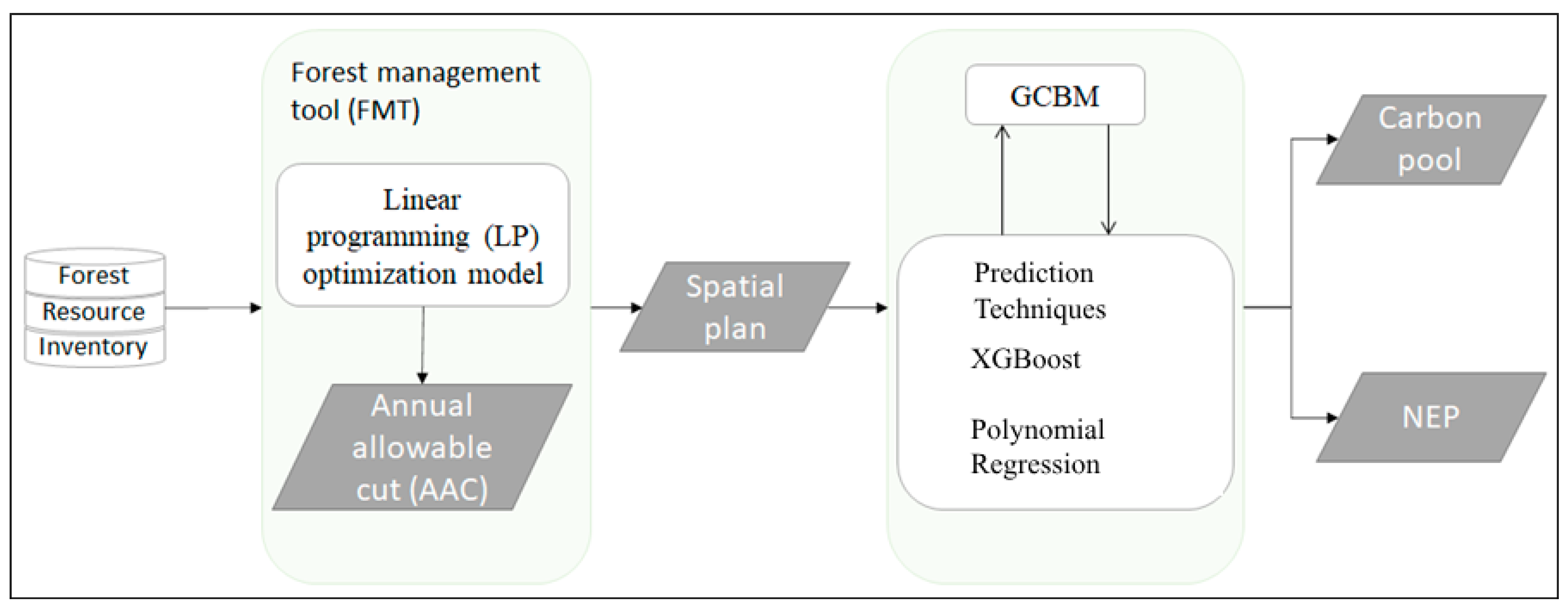
The methodology adopted in this study is summarized in Figure 1. First, the AACs for each study area were calculated using forest resource inventory data and a linear programming (LP) optimization model. Forest management tool (FMT) [29] was used to generate spatial output based on the aspatial solution generated by the LP model. Next, the GCBM model was used to estimate NEP and the carbon pool for the spatial solution. The carbon pool includes aboveground biomass, belowground biomass, deadwood, litter and soil carbon content. The output generated by GCBM was used to train the XGBoost (Extreme Gradient Boosting), a machine learning algorithm. As an added validation benchmark, polynomial regression was also carried out. The NEP and carbon pool were subsequently predicted using the trained ML model to evaluate their performance. A description of the study area is provided in the next subsection followed by description of AAC and carbon calculations, data preparation methods, and model building and evaluating procedures.

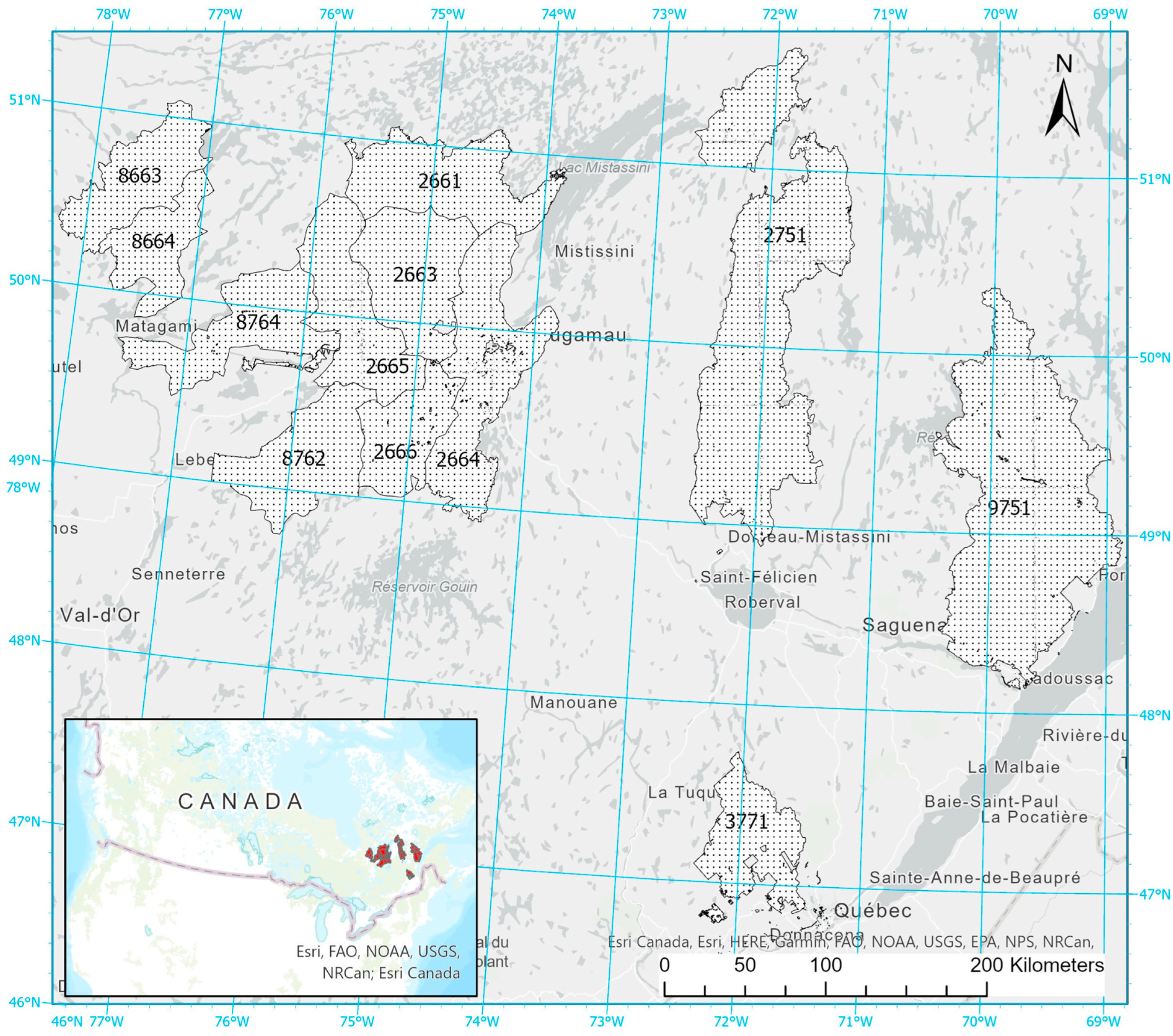
2.1. Study Area

This study was conducted in the province of Quebec, Canada where 12 management units (MUs) were selected from the following administrative regions: Côte Nord, Saguenay-Lac Saint-Jean, Capitale-Nationale and Nord-du-Québec (Figure 2). All 12 MUs are predominantly situated within the Canadian boreal forest and mostly consist of conifer tree species. The total area within each MU and their respective managed and unmanaged forest areas are presented in

Table 1. List of managed, unmanaged and total areas within the management units selected for the study.

Site	Management Unit	Area Designated for Forest Management		Area Excluded from Forest Management		Total Area (Hectare)
		Hectare	%	Hectare	%
Nord-du-Québec	2661	298,200	60	201,470	40	499,670
	2663	99,390	34	193,240	66	292,630
	2664	311,440	81	73,120	19	384,560
	2665	258,960	87	39,250	13	298,210
	2666	161,600	86	26,410	14	188,010
	8663	40,400	22	141,760	78	182,160
	8664	102,280	65	54,350	35	156,630
	8762	265,940	87	38,310	13	304,250
	8764	249,620	90	26,230	10	275,850
Saguenay-Lac Saint-Jean	2751	819,670	83	170,920	17	990,590
Capitale-Nationale	3771	214,810	73	78,370	27	293,180
Côte Nord	9751	909,490	73	335,100	27	1,244,590

.

2.2. AAC and Carbon Calculations

First, AAC was determined using LP model II in the Woodstock Forest modeling system [30]. The output of the AAC was the determination of the maximum volume that can be harvested in the MU per period, by species. As such, it disregarded the spatial aspect. FMT was used to spatialize the disturbances and forest inventory at a 14.4 ha resolution. FMT is an open-source object-oriented library in C++ and was used through the Python programming language version 3.12 for spatial interpretation of Woodstock output.

Next, GCBM was used for carbon calculations as it is designed specifically to evaluate the carbon stock and fluxes of a forest [20]. The spatially explicit plan generated by Woodstock and FMT was input into GCBM along with yield curves, forest inventory data and historical disturbance information to simulate tree growth-related changes in the carbon stock. GCBM also takes into consideration aboveground and belowground biomass, deadwood biomass, litter and soil carbon based on the forest management practice adopted. It explicitly considers biomass mortality dynamics by accounting for the transfer from living to dead biomass [31]. It also incorporates the carbon emission due to the decomposition of dead biomass or direct oxidation within the atmosphere caused by fire disturbance. The list of variables essential to run the GCBM is listed as an Appendix A (

Table A1. List of independent variables essential to run GCBM and machine learning algorithms for prediction of carbon pool and NEP.

S.N.	Net Ecosystem Productivity (NEP) Variables	Acronym
1	Time in the period of 5 years since the last disturbance of the source development	S1_distance
2	Last source disturbance	S1_disturbance
3	Time in the period of 5 years since the penultimate disturbance of the source development	S2_distance
4	Penultimate source disturbance	S2_disturbance
5	Time in the period of 5 years since the disturbance of the source development	S3_distance
6	Source disturbance	S3_disturbance
7	Source development age (age counted in 5-year periods)	Source_age
8	Volume of intolerant hardwood per hectare of source development (m3 ha−1)	Source_YV_G_GFI
9	Volume of tolerant hardwood per hectare of source development (m3 ha−1)	Source_YV_G_GFT
10	Volume of softwood per hectare of source development (m3 ha−1)	Source_YV_G_GR
11	Volume of hardwood per hectare of source development (m3 ha−1)	Source_YV_G_GF
12	Time in the period of 5 years since the disturbance occurred after the source period	Target_distance
13	Type of disturbance occurred between the source and the target period	Target_disturbance
14	Target development age (age is counted in 5-year periods)	Target_age
15	Volume of intolerant hardwood per hectare of target development (m3 ha−1)	Target_YV_G_GFI
16	Volume of tolerant hardwood per hectare of target development (m3 ha−1)	Target_YV_G_GFT
17	Volume of softwood per hectare of target development (m3 ha−1)	Target_YV_G_GR
18	Volume of hardwood per hectare of target development (m3 ha−1)	Target_YV_G_GF
	Carbon pool variables	Acronym
1	Time in the period of 5 years since the last disturbance of the source development	S1_distance
2	Last source disturbance	S1_disturbance
3	Time in the period of 5 years since the penultimate disturbance of the source development	S2_distance
4	Penultimate source disturbance	S2_disturbance
5	Time in the period of 5 years since the disturbance of the source development	S3_distance
6	Source disturbance	S3_disturbance
7	Source development age (age counted in 5-year periods)	Age
8	Volume of intolerant hardwood per hectare (m3 ha−1)	YG_G_GFI
9	Volume of tolerant hardwood per hectare (m3 ha−1)	YG_G_GFT
10	Volume of softwood per hectare (m3 ha−1)	YG_G_GR
11	Volume of hardwood per hectare (m3 ha−1)	YG_G_GF

). The next step required was to train machine learning algorithms to partly substitute for GCBM. As mentioned earlier, one of the significant limitations of GCBM is its high computational requirements. This can make it more challenging for forest practitioners to evaluate multiple scenarios.

2.3. Data Preparation and Dimensionality Reduction

This section provides a detailed description of the data preprocessing that serves as the inputs for the machine learning algorithms. The independent variables for the machine learning algorithms were the same as those used in GCBM (Table A1). This is because GCBM is a state-of-the-art spatial forest carbon model which considers different relevant inputs for its operation [10]. A total of 7.56 million samples were compiled for NEP forecasting and 13.53 million samples for carbon pool prediction. For validation purposes, the effectiveness of the machine learning algorithm was compared to the output of GCBM. Here, the objective was to predict the NEP and the carbon pools; therefore, it was deemed important to apply two different preprocessing approaches. For NEP forecasting, we selected two forest strata because it measures the carbon flux between two periods. For the carbon pool, a single stratum was used because it measures the amount of carbon stored at a given period. The selection of strata was followed by a data cleaning phase. Initially, duplicates as well as null or “NaN” were removed from the list of dependent and independent variables. After the elimination of “NaN” and duplicates, there were approximately 6.77 million samples with 18 independent variables for NEP forecasting and 13.52 million samples with 11 independent variables for carbon pool forecasting. Even after eliminating duplicates and null entries, the dataset was sufficiently large and considered adequate for training and testing the machine learning models.

Since the numbers of dependent variables were large i.e., 18 for NEP and 11 for carbon pools, Principal Component Analysis (PCA) was conducted as a dimensionality reduction technique. It is a technique for simplifying large datasets by transforming them into a lower dimensional space while retaining most of the original information. It works by identifying new axes which are called principal components. Principal components capture the maximum variance in the data, with each component being orthogonal (uncorrelated) to the others [32].

Initially, the data was standardized to have a mean of zero and unit variance using the StandardScaler from the sklearn.preprocessing module. PCA was then applied via the PCA class from sklearn.decomposition. A total of 5 principal components for carbon pool and 6 principal components for NEP were selected as they explained about 85% of the cumulative explained variance of the original data. The transformed principal components were subsequently used for downstream analysis. Then, the dataset was randomly split into two parts, i.e., training (80% of data) and testing (20%), using Scikit-learn with a fixed random seed (random_state = 42). This criterion was adopted for both NEP and carbon pool forecasting.

2.4. Model Selection

In this study, Extreme Gradient Boosting (XGBoost) was used to predict the carbon pool and NEP. To serve as a validation benchmark, polynomial regression was also used to predict the independent variables. A detailed description of the regression techniques utilized is given in the subsection below.

2.4.1. Polynomial Regression

A polynomial regression is a special type of multiple linear regression in which a curvilinear relationship is established between independent and dependent variables (Maulud and Abdulazeez 2020) [33]. The polynomial regression is given as:

$$y={\beta }_0+{\beta }_{1}x+{\beta }_2{x}^2+\cdots +{\beta }_n{x}^n+\mathsf{\in }$$

(1)

where y is the intended outcome (NEP and carbon pool) and β₀ is the intercept, while β_n represents the slope for each explanatory variable x (from Table A1) and ∊ is the error.

One of the major drawbacks of polynomial regression is its inability to deal with the presence of outliers within the dataset, which is believed to reduce performance of these models. Nevertheless, this study uses polynomial regression as a benchmark model and compares prediction with XGBoost.

For polynomial regression model building, the dataset was first split into training (80%) and testing (20%). To determine the optimal model complexity, a systematic grid search was conducted over polynomial degrees from 1 to 4. Similarly, the model was regularized with alpha values of 0.01, 0.1, 1, 10 and 100 using RidgeCV. The parameter combination of polynomial degree and regularization parameter yielding the highest R² value was selected as the best model.

2.4.2. XGBoost

XGBoost is a powerful machine learning algorithm based on the gradient boosting framework and belongs to the family of ensemble learning methods. In this model, a series of decision trees are built, in which each tree attempts to correct the mistakes of the previous one. It incorporates features like regularization, which helps to prevent overfitting, and parallelization, which enables parallel computation during tree construction. Because of these advantages, it is an ideal choice for large-scale datasets due to its significantly faster performance compared to many other implementations. Despite its advantages, XGBoost can still be prone to overfitting if not properly tuned, particularly when dealing with noisy data [34].

2.5. Model Building

XGBoost regression was implemented using the XGBRegressor class from the xgboost python package. To accelerate model training, a histogram-based tree construction algorithm was used in conjunction with GPU acceleration using cuda.

For hyperparameter tuning, a Bayesian optimization approach was employed using the BayesSearchCV utility from the scikit-optimize library to find the best parameter from the given range of possible alternatives (

Table 2. Hyperparameter search space used for Bayesian optimization of the XGBoost model.

Hyperparameter	Range
n_estimators	100 to 500
max_depth	3 to 15
learning_rate	0.01 to 0.3 (log-uniform)
subsample	0.6 to 1.0
colsample_bytree	0.6 to 1.0

). Bayesian optimization uses a probabilistic model to make informed decisions about where in the parameter space to sample next. It focuses on regions of the parameter space that are more likely to yield performance improvements based on the prior observations. Since Bayesian optimization avoids wasting resources on unpromising combinations, it is sample-efficient and faster [35].

Three-fold cross validation was used for internal performance validation. Since XGBoost is a tree-based algorithm, it is not sensitive to the scale of the features. Hence, data transformation methods like standardization and normalization are not required as tree-based models divide the data based on feature thresholds, not distance or magnitude [36]. Since PCA was already applied in advance, which required data scaling, no further data transformation was carried out for XGBoost.

As machine learning models are susceptible to overfitting and susceptible to noisy data, some precautions were also taken into account. First, the incorporation of PCA as a dimensionality reduction step helped to reduce feature collinearity and noise, in turn improving generalization. Likewise, as mentioned previously in the description of the XGBoost model, its inherent ensemble structure and decision tree-based approach are comparatively less sensitive to noisy or unscaled features, as splits are based on thresholds rather than distances.

2.6. Model Evaluation Criteria

Three metrics, namely coefficient of determination (R²), mean absolute error (MAE), and root mean squared error (RMSE), were used to evaluate overall model performance. The coefficient of determinants, R², is an extensively used evaluation metric for a variety of applications [37]. The R² value ranges between 0 and 1 and the model is considered to be effective if its value is close to 1. The two other metrics, namely RMSE and MAE, measure the deviation of modelled output from the observed value. The values of both MSE and MAE range between 0 and ∞ and the model with a value close to 0 is regarded as the best-performing. Among these three indicators, the R² was the main performance metric used to assess performance of tested models. It is also worth pointing out that the results obtained with the testing dataset are linked to its distribution and it is impossible to guarantee that another dataset with completely different distributions would yield the same results. It should also be noted that all the processing was carried out in the Python programming language within the Anaconda environment using the sklearn package. Likewise, to determine the robustness of the model across different data partitions, a repeated sub sampling method was implemented using the ShuffleSplit method from the scikit-learn library. The methodology involved generation of 10 independent train–test splits (80–20 ratio). For each split, the machine learning model was retrained using the optimal hyperparameters previously identified through the Bayesian optimization and evaluated using the performance metrics.

3. Results

3.1. GCBM Predictions

Predictions of different carbon pool components and the net ecosystem productivity for the 12 management units derived from the GCBM model are shown in Figure 3. Generally, GCBM uses around 3.5 min per million simulations and predicts the NEP and carbon pools. Note that each prediction represents a forest stratum. The time taken by GCBM may vary by ±1 min depending upon the composition of the forest strata used. The violin plot shows the descriptive statistics of results from the year 2023 to 2158, broken down into 5-year periods. The width of the violin plot reflects the data’s distribution density, with wider sections indicating a higher frequency of observations. The central box plot conveys measures of central tendency and variability. Symbols and colors have been arbitrarily assigned to differentiate between various MUs. It predicted the annual average carbon stock (tonne ha⁻¹) of aboveground biomass, belowground biomass, deadwood, litter and soil carbon. Also shown in the figure is the annual average carbon flux, i.e., net ecosystem productivity (tonne CO_2e ha⁻¹ year⁻¹). Each subplot shows a noticeable amount of variability in carbon metrics and the net ecosystem productivity. This is due to the fact that our data contains variable forests with different age classes, even and uneven-aged forest management practice, climatic differences and disturbances. The majority of the carbon was stored on the ground or below (belowground biomass, deadwood, litter and soil). Nevertheless, aboveground biomass represents an important proportion of the carbon as well. When observing Figure 3, site-wise variability in the carbon pools and flux (NEP) is observed. During most of the time period (2023–2158), there is a great variability among each MU stratum. As an example, most of those strata show a negative NEP value, meaning that they act like carbon sources. However, strata producing emissions, which can be attributed to harvesting and other silvicultural treatments, represent a small portion in each MU. A high proportion of area in each MU is experiencing growth, so this is most likely the explanation for the carbon sink seen in these strata.

3.2. Descriptive Statistics

The descriptive statistics for the NEP are shown in

Table 3. Descriptive statistics of the variables for NEP estimation.

SN	Variable	Description	Unit	Mean	Variance
1	s1_distance	Time since last source disturbance	5-year period	13.5609	163.9410
2	s1_disturbance	Last source disturbance	5-year period	3.6453	17.6253
3	s2_distance	Time since penultimate source disturbance	5-year period	17.1715	296.9884
4	s2_disturbance	Penultimate source disturbance	5-year period	9.2516	43.8843
5	s3_distance	Time since source disturbance	5-year period	8.5932	254.3553
6	s3_disturbance	Source disturbance	5-year period	14.0496	29.2366
7	source_age	Age of source development	5-year period	13.6820	170.1568
8	source_YV_G_GFI	Volume of intolerant hardwood per hectare	m3/ha	11.5353	624.1651
9	source_YV_G_GFT	Volume of tolerant hardwood per hectare	m3/ha	6.8136	836.8290
10	source_YV_G_GR	Volume of softwood per hectare	m3/ha	43.4437	3144.2515
11	source_YV_G_GF	Volume of hardwood per hectare	m3/ha	18.3489	1626.6555
12	target_distance	Time since disturbance at target	5-year period	0.9383	0.0579
13	target_disturbance	Most recent disturbance at target	5-year period	15.1268	12.0259
14	target_age	Age of target stand	5-year period	13.6366	169.9266
15	target_YV_G_GFI	Target: intolerant hardwood volume	m3/ha	11.4001	602.9208
16	target_YV_G_GFT	Target: tolerant hardwood volume	m3/ha	6.7364	824.7986
17	target_YV_G_GR	Target: softwood volume	m3/ha	43.3258	3219.2981
18	target_YV_G_GF	Target: hardwood volume	m3/ha	18.1365	1591.1015
19	NEP *	Net ecosystem productivity	tonne CO2e ha −1 year −1	0.1540	1.5648

* Dependent variable.

and those for the carbon pool are shown in

Table 4. Descriptive statistics of the independent variables for carbon pool estimation.

SN	Variable	Description	Unit	Mean	Variance
1	s1_distance	Time since last source disturbance	5-year period	13.5207	164.7908
2	s1_disturbance	Last source disturbance	5-year period	3.5666	17.3322
3	s2_distance	Time since penultimate source disturbance	5-year period	17.7052	292.3556
4	s2_disturbance	Penultimate source disturbance	5-year period	9.0615	43.7595
5	s3_distance	Time since source disturbance	5-year period	9.3789	259.8389
6	s3_disturbance	Source disturbance	5-year period	13.9239	30.1450
7	age	Age of source development	5-year period	13.6564	169.9665
8	YV_G_GFI	Volume of intolerant hardwood per hectare	m3/ha	11.4687	613.4764
9	YV_G_GFT	Volume of tolerant hardwood per hectare	m3/ha	6.7712	830.0655
10	YV_G_GR	Volume of softwood per hectare	m3/ha	43.3799	3183.7146
11	YV_G_GF	Volume of hardwood per hectare	m3/ha	18.2399	1608.0060
12	AG_Biomass_C *	Aboveground biomass	tonne ha−1	30.955	774.117
13	BG_Biomass_C *	Belowground biomass	tonne ha−1	8.008	42.046
14	Deadwood_C *	Deadwood	tonne ha−1	11.322	53.018
15	Litter_C *	Litter	tonne ha−1	43.506	449.052
16	Soil_C *	Soil carbon	tonne ha−1	79.639	1039.982

* Dependent variables.

. Each of the variables were of continuous data type.

3.3. Machine Learning Results

For our simulation, we used an i9-10900K processor computer with 64GB RAM and NVIDIA GeForce RTX 3080 graphics card. On average, it took approximately 35 min to train one dependent variable in the XGBoost model. After the Bayesian optimization process found the best parameters for the training (

Table 5. Best set of hyperparameters obtained after Bayesian optimization of the XGBoost model.

Target	Colsample_Bytree	Learning Rate	Max Depth	N Estimators	Subsample
NEP	1.0	0.1462	15	424	1.0
AGB	1.0	0.1752	15	500	1.0
Belowground	1.0	0.2987	15	500	1.0
Deadwood	1.0	0.3000	15	299	1.0
Litter	1.0	0.3000	15	346	0.8966
Soil carbon	1.0	0.3000	15	346	0.8966

), it took approximately 45 s to predict the NEP and the carbon pools. Although the polynomial regression was the worst performing model, the computational requirement was insignificant as it only took on average a minute to train the model.

In the case of NEP, XGBoost was significantly better and outperformed polynomial regression in all of the metrics, i.e., R², RMSE and MAE (

Table 6. Performance evaluation metrics comparison between XGBoost and the polynomial regression model for prediction of NEP.

Metric	XGBoost	Polynomial Regression
R2	0.883	0.678
RMSE	0.428	0.708
MAE	0.196	0.471

). XGBoost yielded a higher R², 0.883, along with lower RMSE and MAE values.

As the carbon pool includes aboveground biomass, belowground biomass, deadwood, litter and soil carbon content, it is important to segregate and identify whether ML models provide good outcomes for these individual variables. Similar to NEP, polynomial regression provided the least favourable outcome as compared to XGBoost when predicting the carbon contents, especially for the deadwood carbon pool component (i.e., R² = 0.496) (Figure 4). Among all the variables, XGBoost also showed less favourable prediction for Deadwood (i.e., R² = 0.872) (Figure 4) while still being significantly better than polynomial regression. Aboveground and belowground biomass were the only two variables which yielded acceptable R² under polynomial regression. XGBoost showed the highest predictive accuracy for aboveground biomass (R² = 0.968) followed by belowground biomass, litter, soil and deadwood. All in all, XGBoost was a comparatively better and more accurate predictive model when evaluated through the metrics of R² (Figure 4), RMSE (Figure 5) and MAE (Figure 6). In the case of polynomial regression, the best degree was found to be 4 in all the instances.

The results of the ShuffleSplit method, which accounts for stability of the model across different data partitions, can be found in Appendix A 

Table A2. Shuffle split cross-validation results (mean ± standard deviation) obtained after ten runs for R², RMSE and MAE across target variables.

Target Variables	R2 (Mean ± std)	RMSE (Mean ± std)	MAE (Mean ± std)
NEP	0.8825 ± 0.0004	0.4289 ± 0.0007	0.1956 ± 0.0002
Aboveground biomass	0.9684 ± 0.0001	4.9520 ± 0.0065	1.8947 ± 0.0031
Belowground biomass	0.9645 ± 0.0001	1.2230 ± 0.0015	0.4871 ± 0.0005
Deadwood	0.8712 ± 0.0009	2.6144 ± 0.0082	1.3259 ± 0.0014
Litter	0.9178 ± 0.0002	6.0740 ± 0.0085	3.4792 ± 0.0042
Soil carbon	0.8970 ± 0.0003	10.3506 ± 0.0128	5.8932 ± 0.0053

. The result is summarized as the mean and standard deviation of the evaluation metrics across the 10 runs. The standard deviation across 10 runs was quite low, indicating that the model’s predictive performance was consistent across different data partitions. Although the training time for polynomial regression was minimal (less than one minute) despite the large dataset, the resulting predictions exhibited considerable variability and low accuracy and reliability across the NEP and carbon pool components. In contrast, XGBoost demonstrated superior performance in predicting both the NEP and carbon pool components with high accuracy. Although XGBoost requires a relatively longer initial training time, it remains within acceptable computational limits.

4. Discussion

To investigate the carbon fluxes and the stock dynamics of managed forests in Quebec, a set of 12 management units were chosen, and subsequently analysed using GCBM, a robust tool for carbon budgeting [10,19,20]. As expected, in these MUs, we observed site-wise variability for carbon pools and NEP. 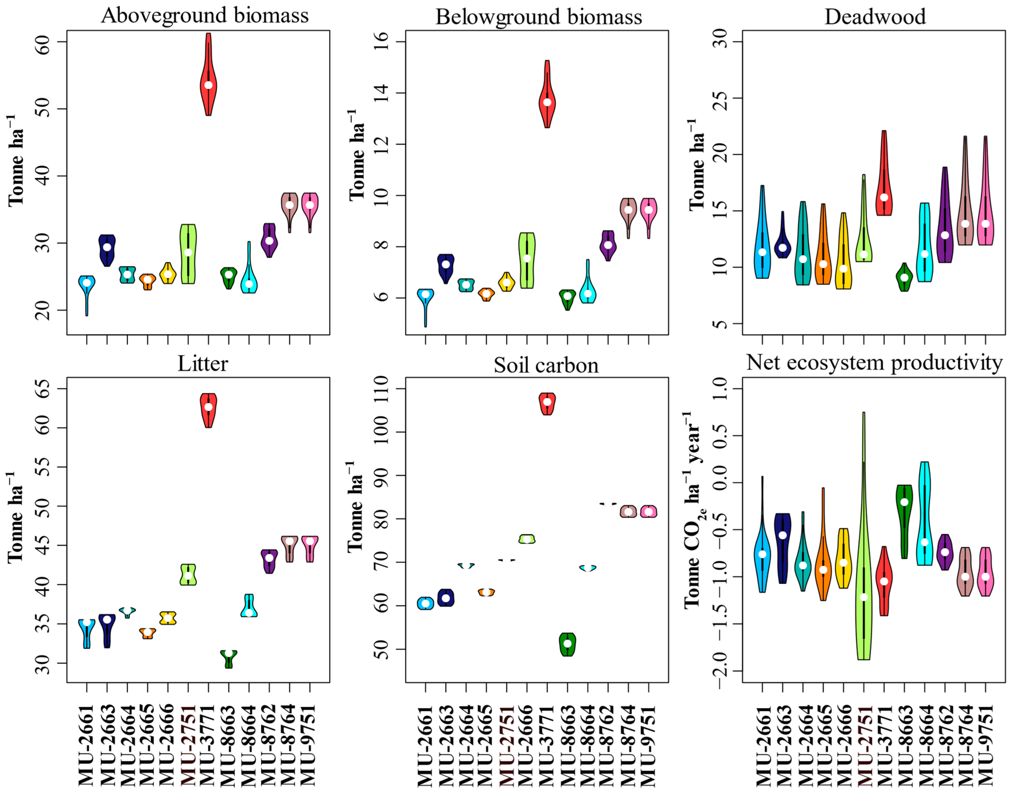Several past studies have already provided detailed information regarding the role of forest age, structure, management, climate and disturbances which cause variability in carbon storage and flux [7,10,14,38,39], as is the case in these MUs. Moreover, our results, illustrated in Figure 3, indicate that the soil stored a significant proportion of carbon while deadwood stored the lowest amount. Our results are comparable to other studies that indicate that boreal forest stores a significant proportion of carbon in soil rather than in vegetation [40,41]. This can be attributed to the reduced organic carbon decomposition rates, particularly in the northern regions with colder climates [40]. The geographical distribution along with the adopted management practices also contributes to the variability in overall carbon content for these individual carbon pool components. These differences contribute to variability in the composition and structure of forests which in turn have substantial influence on soil carbon properties [42].

Based on the GCBM model results, MU-3771, located in Capitale-Nationale, exhibited greater mean carbon stock (Figure 3) than all other management units. As displayed in Figure 1, MU-3771 is situated in the southernmost region. Here, a favorable climate supports the existence of mixed wood forests. Such diverse forests often have an effective ability to capture a significant proportion of carbon [43]. For instance, [44] compared the variability in soil carbon sequestration potential for temperate and boreal forest tree species. The authors concluded that mixed forests had larger potential to store soil carbon than the spruce forest. On the contrary, it is also worth pointing out that the northern forests, with less diverse tree species, showcased variability in carbon pools. Several past studies have already highlighted the importance of species composition and carbon capture. Therefore, one can see the variability in the carbon pools across our management units. We also evaluated the NEP values derived using GCBM. Most of the strata had a negative NEP value which can be explained by logging activities that took place in the area [45], or the successional stage (late) of the forests [46,47]. The MUs are mostly viewed as carbon sinks over the long term > 100 years [31]. Our data is composed of a majority of carbon source strata, but these only represent a small amount of area for each MU.

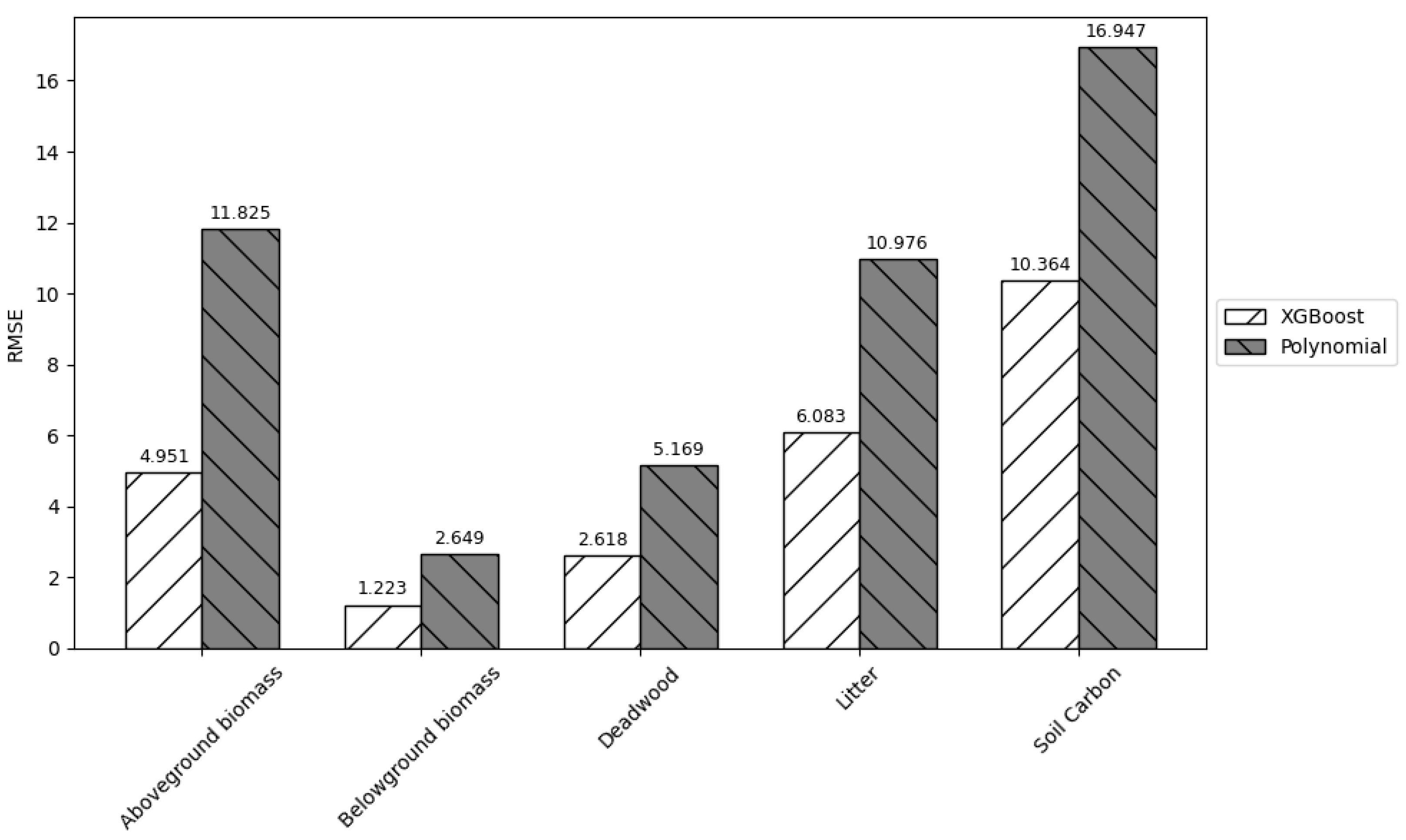
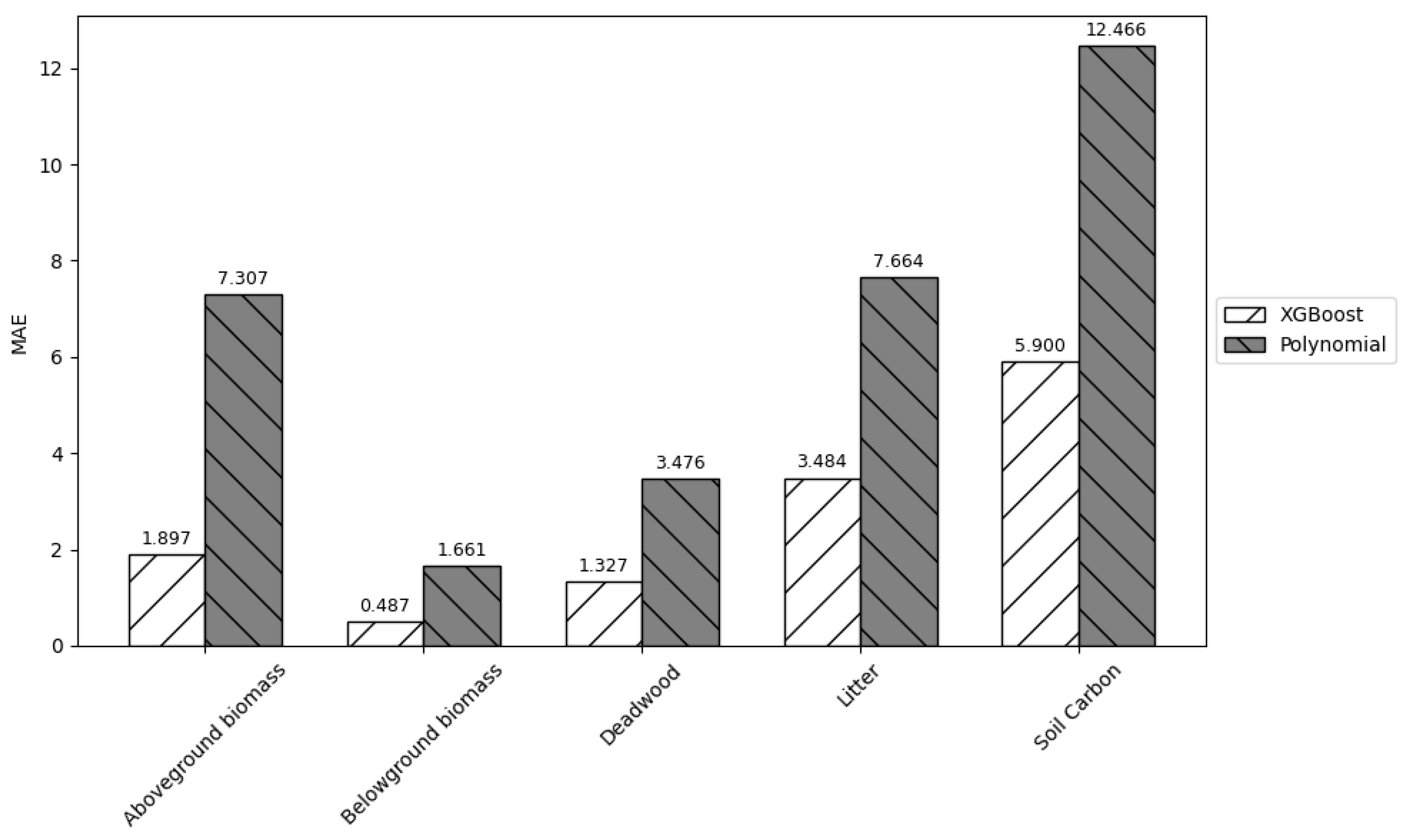
Likewise, the results indicate that XGBoost model was effective in replicating the results of the GCBM model. The model demonstrated high accuracy and generalization capacity, as evidenced by the R² value. XGBoost’s success as compared to the normal polynomial regression can be largely attributed to its ability to efficiently handle large datasets, and its superior abilities to capture non-linear feature interactions and mitigate overfitting through integrated regularization mechanisms [34]. Among the predicted variables, aboveground and belowground were predicted with the highest accuracy with R² exceeding 0.96. Litter and soil carbon also exhibited high predictive performance with values around 0.90. NEP and deadwood had relatively lower predictive performance as compared to the others. Nevertheless, these deviations are minor, and the overall performance still remained within the acceptable limits. This variation is likely due to the inherent variability within the individual dataset and measurement uncertainty across the individual components.

A critical factor in achieving high model performance is the careful selection and tuning of hyperparameters, as the accuracy of a machine learning model is highly dependent upon the appropriate hyperparameters. While the hyperparameter space was optimized to a practical extent, the process was constrained by the computational burden posed by the large dataset. A wider search could have potentially improved the model accuracy even further; however, it was limited by time and hardware restrictions. Hence, there should be an optimal balance of computational efficiency and model accuracy.

Moving towards computational efficiency, other machine learning algorithms, particularly random forest and artificial neural networks, were also considered in the pilot phase, but ultimately discarded due to their relative inefficiency in handling large datasets. In preliminary comparisons, it took more than 4 h to train a single dependent variable for an artificial neural network as compared to XGBoost, which only took an average of 30 min. Likewise, random forest also took more than 7 h in the training phase. In addition to this, ANNs, while offering high representational capacity, are also sensitive to data transformation methods like scaling and normalization and require extensive training time. Hence, XGBoost was selected as the best machine learning model in our pilot study phase which offered a good balance of accuracy and efficiency.

It seems that XGBoost is best suited for scenarios where rapid decision-making is required, such as generating multiple forest management scenarios in tactical planning, conducting preliminary carbon assessments, or supporting stakeholder engagement through scenario comparison. Its speed and scalability make it particularly advantageous when hundreds or thousands of alternative management scenarios must be evaluated quickly. However, XGBoost is not a replacement for GCBM in contexts that demand high precision, or mechanistic understanding of carbon dynamics, for instance, in regulatory reporting, policy evaluation, carbon credit verification or long-term national carbon accounting. GCBM remains more suitable when detailed representations of ecological processes, forest succession, and disturbance interactions are critical. Therefore, we recommend a hybrid use, where XGBoost can rapidly screen options and GCBM is applied to a select set of high-priority scenarios for more robust carbon evaluation.

The objective of this study was to achieve the maximum possible accuracy within an acceptable time frame. Note that the models presented in this study exclusively rely on the datasets from the management units in Quebec. While the XGBoost model developed in this study demonstrated high predictive accuracy within Quebec’s boreal forest context, its applicability to other forest regions needs to be evaluated. The model was trained using region-specific variables, forest inventory data, disturbance regimes and climatic conditions unique to Quebec’s boreal forest. As such, applying the model to other provinces or countries with different ecological characteristics, forest compositions or management practices could lead to reduced accuracy. Model retraining or transfer learning with local data from other places should be used in future work to examine the transferability and applicability of the model in other ecological contexts.

5. Conclusions

The Generic Carbon Budget Model (GCBM) is a robust and widely utilized tool used for simulating carbon stocks and fluxes in forest ecosystems. However, its high computational demand poses a significant barrier for rapid scenario assessments, limiting its practical integration into dynamic forest management planning workflows. To address this limitation, we investigated the potential of machine learning, specifically XGBoost, to predict key carbon metrics. Our results demonstrated that XGBoost can effectively replicate the output of GCBM with high accuracy while drastically reducing computation time. For instance, the trained model achieved R² values of 0.883 for NEP and 0.967 for aboveground biomass carbon. It was able to predict millions of outputs in less than a minute after model training. Polynomial regression, used as a benchmark, consistently underperformed as compared to XGBoost, further validating the model’s suitability.

Based on the results, it is proposed that machine learning models like XGBoost are suitable for tasks that involve rapid evaluation of multiple forest management scenarios. GCBM, in contrast, remains better suited for applications which demand high accuracy. A hybrid approach using a machine learning model to filter a wide set of management options and then applying GCBM to a smaller subset could offer a promising pathway for balancing speed and precision in carbon-informed forest planning.

Practically, our findings suggest that machine learning can be effectively integrated into existing spatial planning workflows to enable faster carbon evaluation without significantly compromising on accuracy. However, care must be taken when applying the trained models outside their original context, as the accuracy of the model is tied to the structure and conditions of the training dataset. For future work, we recommend developing streamlined methods to integrate ML models like XGBoost directly into forest planning tools. In addition, more extensive benchmarking against other machine learning algorithms and application of the model to forest regions outside Quebec would further test its generalizability and operational utility.