Sustainable Distribution Network Planning for Enhancing PV Accommodation: A Source–Network–Storage Coordinated Stochastic Approach

Abstract

To address the impacts of source load temporal–spatial uncertainties on distribution network planning considering the global transition towards sustainable energy systems with high-penetration photovoltaic (PV) integration, this paper proposes a source–network–storage coordinated stochastic planning method. A temporal–spatial correlation probability model for PV output and load demand is constructed based on Copula theory. Scenario generation and efficient reduction are achieved through Monte Carlo sampling and K-means clustering, extracting representative daily scenarios that preserve the temporal–spatial characteristics. A coordinated planning model targeting the minimization of comprehensive costs is established to holistically optimize PV deployment, energy storage system (ESS) configuration, and network expansion schemes. Simulations on typical distribution network systems demonstrate that the proposed method, by integrating temporal–spatial correlation modeling and multi-element collaborative decision-making, significantly improves PV accommodation capacity and reduces planning costs while improving the overall economic efficiency of distribution network planning. This study provides a robust technical pathway for developing economically viable and resilient distribution networks capable of integrating large-scale renewable energy, thereby contributing to the decarbonization of the power sector and advancing the goals of sustainable energy development.

1. Introduction

With the vigorous development and utilization of PV in distribution networks [1,2], the uncertainty of its output and the volatility of loads have brought great challenges to the balance of energy supply and demand [3]. At the same time, the load growth requires the expansion of the distribution network framework, and the unreasonable structure will seriously affect the operation of the system [4,5]. The ESS has the ability of bidirectional regulation [6]. The collaborative planning of ESS and PV can greatly improve the utilization rate of PV [7,8]; optimize resource allocation; and improve the reliability, security, and flexibility of distribution network operation [9,10]. Therefore, considering the uncertainty of PV output and load demand, it is of great practical significance to study the distribution network planning scheme, including site selection and capacity determination of PV and ESS, as well as network expansion.

Currently, a large number of scholars have conducted in-depth research on the planning problem of distribution networks. Reference [11] proposed a novel hybrid optimization algorithm that combines clonal selection principle and particle swarm optimization to optimize the capacity and location of DG in the power system. References [12,13,14] studied the optimal allocation of ESS with the aim of improving system economy. The above literature has only modeled the distribution network planning problem considering the optimal allocation of DG or ESS. In distribution network planning, however, the joint planning of PV and ESS is of great significance to enhance the capacity of a distribution network to consume the power generation of PV and reduce the loss of resources [15,16]. Reference [17] employed PSO for optimal PV–DG and BESS allocation, enabling dynamic and static network reconfiguration to minimize losses, improve voltage profiles, and enhance system loadability. Reference [18] established a two-step approach to configure the power and capacity of the ESS through scheduling and control strategies. Reference [19] proposed a bi-level programming approach and developed an improved binary particle swarm optimization algorithm based on chaos optimization to achieve the optimal joint planning of DG and ESS. There have been many studies on the distribution network planning problem for the optimal allocation of DG and ESS, but few studies have fully investigated the model for the collaborative planning of source–network–storage.

The randomness of load and PV will pose a great challenge to the planning of distribution networks [20]. To address the uncertainty problem of load and PV, Reference [21] proposed a time series-based planning method for modeling the load demand and PV output variations in a single day. In order to solve the time series model containing PV, the study adopted the Monte Carlo method to simulate different scenarios by random sampling to obtain more accurate planning results. The method takes into account time series changes, but because it does not consider the different load demand and PV output of different days, it results in less accurate planning results. Reference [22] established a coordinated planning model for distributed wind power and transmission lines by comprehensively considering investment costs, environmental benefits, and power supply reliability. However, under this planning framework, the generator output is assumed to be constant, which deviates from real-world conditions and fails to account for uncertainty. To address the uncertainty problem of multiple scenarios, Reference [23] proposed a wind power scenario simulation method to analyze the random characteristics of wind power output, integrating improved forecasting, nonparametric kernel distribution, and a BR scene reduction model.

In summary of the above research and analysis, this paper first establishes a probabilistic model of source load temporal–spatial correlation based on Copula theory to deal with the randomness of the PV outputs and load and generates the source load correlation output curves of a typical daily scenario by the Monte Carlo method and K-means clustering algorithm. Then, aiming at enhancing the efficient consumption of PV and the economics of distribution network planning, the collaborative planning of source–network–storage is studied based on stochastic scenarios, and the joint planning model of PV, ESS, and grid expansion is established. Finally, the effectiveness of the proposed method to improve the PV absorption capacity and the economy of distribution network planning is verified by simulation analysis of 25-node and 54-node arithmetic examples.

2. Source Load Temporal–Spatial Correlation Scenarios

2.1. Probabilistic Model of Source Load Temporal–Spatial Correlation Based on Copula Theory

In the correlation coefficient discriminant, Kendall correlation coefficient and Spearman correlation coefficient [24] are often used to assess the goodness of fit. Both of the rank correlation coefficients are statistical analyses that reflect the degree of rank correlation and are used to measure the degree of association between two variables. In the goodness of fit discrimination of Copula functions, the rank correlation coefficients of each Copula function can be compared with the rank correlation coefficients of the sample data. By calculating these correlation coefficients and observing how close they are to the correlation coefficients of the sample data, the goodness of fit of the Copula function to the sample data can be assessed. The closer the data, the better the fit, indicating that the corresponding Copula function is the most appropriate. This approach helps to select the most suitable model to characterize the data among multiple Copula functions.

Let the load and PV output be U and V, respectively. (u₁, v₁) and (u₂, v₂) are any two sample observations of its output (U, V). The two values are independent of each other. If (u₁, v₁)·(u₂, v₂) > 0, then (u₁, v₁) and (u₂, v₂) are considered consistent; otherwise, (u₁, v₁) and (u₂, v₂) are considered inconsistent.

Kendall rank correlation coefficient is ρ_k

$${\rho }_{\mathrm{k}}={\displaystyle \frac{2(a-b)}{N(N-1)}}$$

(1)

where a denotes the number of pairs of samples with consistent output in (U, V); b denotes the number of pairs of samples with inconsistent output in (U, V); N denotes the total number of sampling points; and N is taken as 24 in this paper, i.e., the step size is 1 h.

Spearman rank correlation coefficient is ρ_s

$${\rho }_{\mathrm{s}}={\displaystyle \frac{{\displaystyle \sum _{i=1}^N(c_i-\overline{c})(d_i-\overline{d})}}{\sqrt{{\displaystyle \sum _{i=1}^N{(c_i-\overline{c})}^2}}\sqrt{{\displaystyle \sum _{i=1}^N{(d_i-\overline{d})}^2}}}}$$

(2)

where c_i denotes the rank of u_i in (u₁, u₂, …, u_N); d_i denotes the rank of v_i in (v₁, v₂, …, v_N): $\overline{c}={\displaystyle \sum _{i=1}^N\frac{c_i}{N}}$; $\overline{d}={\displaystyle \sum _{i=1}^N\frac{d_i}{N}}$.

The Euclidean distance discriminant [25] is an effective method to assess the similarity or difference between objects in a multidimensional space. The Euclidean distance discriminant also plays an important role in the goodness of fit discrimination of Copula functions. This method compares the Euclidean distance of each Copula function with the Euclidean distance of the empirical Copula function for the sample data. The calculation of the Euclidean distance is based on the formula of the distance between points in a multidimensional space, which measures the sum of the differences between two points in each dimension. Here, each Copula function and the empirical Copula function of the sample data can be regarded as points in a multidimensional space with dimensions determined by the parameters of the Copula function or other relevant features.

By comparing these Euclidean distances, it is possible to conclude which Copula function provides a better fit to the sample data. In general, the smaller the Euclidean distance is, the closer the two objects are in the multidimensional space, i.e., the more similar they are. Therefore, the smaller the Euclidean distance is, the more similar the Copula function is to the empirical Copula of the sample data, and the better the fit is.

Let (x_i, y_i) (i = 1, 2, …, n) be a sample of the (X, Y) two-dimensional variable and F_n(x_i) and F_n(y_i) be the empirical cumulative distribution functions of the two-dimensional variable (X, Y), respectively. The empirical Copula function for the sample is calculated as

$$C_n(u,v)={\displaystyle \frac{1}{n}}{\displaystyle \sum _{i=1}^n{I}_{[F_n\left(x_i\right)⩽u]}{I}_{[G_n\left(y_i\right)⩽v]}}$$

(3)

where $I_{[\cdot ]}$ denotes the characteristic function. When $F_n(x_i)⩽u$, there exists $I_{[F_n\left(x_i\right)⩽u]}=1$; otherwise, $I_{[F_n\left(x_i\right)⩽u]}=0$. It is the same for $I_{[G_n\left(y_i\right)⩽v]}$.

The most appropriate function is discriminated by comparing the magnitude of the squared Euclidean distance:

$$d^2={\displaystyle \sum _{i=1}^n{\left|C_n(u_i,v_i)-C_e(u_i,v_i)\right|}^2}$$

(4)

where $u_i=F_n(x_i)$, $v_i=G_n(y_i)$. $C_e(\cdot )$ denotes the empirical Copula function. The smaller $d^2$ is, the better the fit of the function.

Nonparametric kernel density estimation is a nonparametric test that characterizes the distribution of data directly from a sample of real data [26]. Assume that the data sample probabilistic density function and its nonparametric kernel density estimation is

$$F(x)={\displaystyle \frac{1}{n}}{\displaystyle \sum _{i=1}^{n}K(x-x_i)}={\displaystyle \frac{1}{nh}}{\displaystyle \sum _{i=1}^{n}K(\frac{x-x_i}{h})}$$

(5)

where x denotes a sample of random variables $x_1,x_2,\dots x_n$; n denotes the sample space; h denotes the window, and h > 0; $K(x)$ denotes the kernel function.

Nonparametric kernel density estimation focuses on the selection of the kernel function and bandwidth. $F(x)$ inherits the continuity and differentiability of $K(·)$, and the window h affects the fit. The kernel function $K(·)$ is a probabilistic density function that conforms to non-negativity, integrates to 1, and has a mean of 0. The commonly used $K(·)$ is the following Gaussian function:

$$K(x)={\displaystyle \frac{1}{\sqrt{2\mathsf{\pi }}}}\exp (-{\displaystyle \frac{1}{2}}{x}^2)$$

(6)

For the construction of the probabilistic model of source load temporal–spatial correlation based on Copula theory, an estimation of parameter θ is required, which can effectively simplify the complex calculation process of the traditional joint distribution model. The estimation of parameter θ adopts the correlation index method, which can be indirectly determined by calculating the correlation index of the samples.

The parameters θ of the Gumbel Copula, Clayton Copula, and Frank Copula functions are estimated by using maximum likelihood. To ensure the accuracy of these parameters, the Kendall rank correlation coefficient τ was further adopted in this paper for testing.

Based on the probabilistic model of the load demand and PV output, while fully considering the temporal–spatial correlation between them, a probabilistic model of source load temporal–spatial correlation is established by using Copula theory. This model can more accurately describe and predict the temporal–spatial correlation between load demand and PV output, which lays the foundation for the planning and operation optimization of distribution networks.

The diagram for generating the probabilistic model of source load temporal–spatial correlation based on Copula theory is shown in Figure 1.

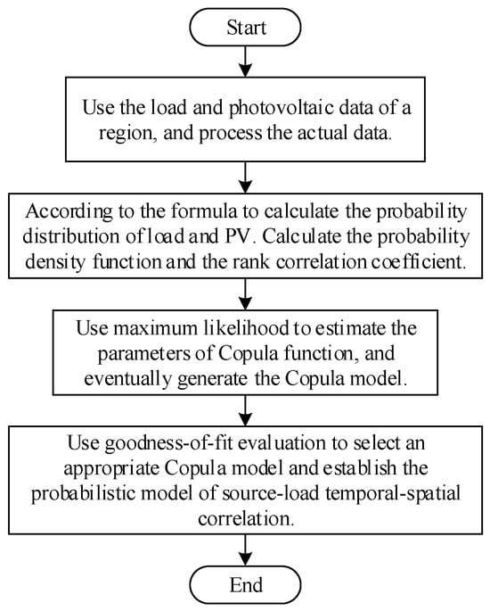
Figure 1. Probabilistic model generation process diagram.

2.2. Scenario Generation Based on the Monte Carlo Method

Scenario generation is a key step in the uncertainty modeling of distribution networks. It aims to quantify uncertainty using deterministic information, thereby constructing discrete probabilistic scenarios that are deterministic. This process relies on probabilistic forecasting and generates a series of scenarios to reflect the uncertainty between the source and load. When selecting uncertainty factors, they usually need to be determined according to specific decision problems. In existing research, factors such as PV generation, load demand, forecasting errors, and variability characteristics are often considered as significant uncertainty factors. This paper specifically focuses on two key factors: PV generation and load demand.

Compared to directly using stochastic programming, the scenario generation method comprehensively describes the uncertainty of source load through a large number of scenarios, making the model closer to the actual planning problem of distribution networks. The generated scenarios can precisely represent the uncertainty probability distribution with discrete deterministic samples, fully reflecting the temporal and spatial characteristics. This method not only improves the accuracy and reliability of the model but also helps optimize the operational decisions of the distribution network, enhancing the overall performance of the power system.

In dealing with the probabilistic model of source load temporal–spatial correlation generated based on Copula theory, this paper employs the Monte Carlo method [27] for scenario sampling to generate a large number of source load temporal–spatial correlation scenarios. The specific steps for generating these scenarios based on the Monte Carlo method are as follows:

After obtaining the probabilistic model of source load temporal–spatial correlation based on Copula theory, we need to perform sampling to generate a large number of samples for subsequent analysis. The main steps of the sampling process are as follows:

(1)

Randomly generate numbers $a_1,a_2,\cdots ,a_n$ within the interval [0, 1].

(2)

$u_1=a_1$ represent the marginal distribution function value of one random variable, and $u_2$ represent the marginal distribution function value of another random variable. $u_2$ can be obtained by the pre-selected optimal Copula function C, calculated by Equation (7):

$${\displaystyle \frac{\partial C\left(u_1,u_2,\dots ,u_n\right)}{\partial u_1}}=a_2$$

(7)

(3)

$u_n$ is the value of the n-th function, which can be determined using Equation (8):

$${\displaystyle \frac{\frac{{\partial }^{n-1}C(u_1,u_2,\dots ,u_n)}{\partial u_1\partial u_2\dots \partial u_{n-1}}}{\frac{{\partial }^{n-1}C(u_1,u_2,\dots ,u_{n-1},1)}{\partial u_1\partial u_2\dots \partial u_{n-1}}}}=a_n$$

(8)

(4)

Repeating the above process k times, it is able to obtain k sets of peripheral distribution function values containing n random variables.

(5)

$(u_{1j},u_{2j},\dots ,u_{nj})$ can be transformed into a joint distribution function scenario by solving the inverse function $x_i=F_i^{-1}(u_i)$, where $j=1,2,\cdots ,T$, and T is the total number of days.

Inverse function calculations are involved in analyzing the correlation between both PV and load. First, the Copula probability model is used to derive the peripheral distribution functions of PV output and load demand. Subsequently, inverse function calculations are performed for each of these two peripheral distribution functions. This approach ensures that the temporal–spatial correlation between PV output and load demand is fully considered in the generated scenarios.

The stages of scene generation are shown in Figure 2.

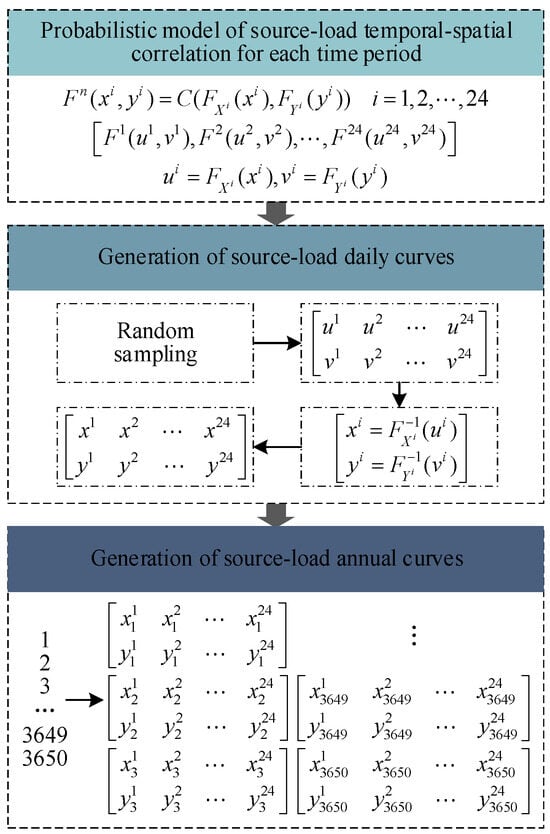
Figure 2. Steps for generating source load temporal–spatial correlation scenarios.

2.3. Scenario Reduction Based on the K-Means Clustering Algorithm

While scenario analysis requires a large number of scenarios to reduce uncertainty, too many scenarios will greatly increase the computational burden of stochastic optimization. Therefore, it is necessary to reduce the large number of scenarios generated by the scenario analysis to a smaller set of representative scenarios, which is called scene reduction. That is, from the given initial scene set S, select some scenes that meet the conditions to form a reserved scene set R, so that the reserved scene set R can be representative as much as possible, and the abandoned scenes form a deleted scene set D.

The main scenario reduction methods include simultaneous backward reduction, fast forward reduction, and clustering analysis methods such as K-means and K-medoids. Although the implementation processes differ, the objective of these reduction methods is consistent. However, when dealing with a large number of scenarios, the K-means clustering algorithm stands out due to its speed advantage in clustering.

The scenario reduction flowchart based on the K-means clustering algorithm is shown in Figure 3.

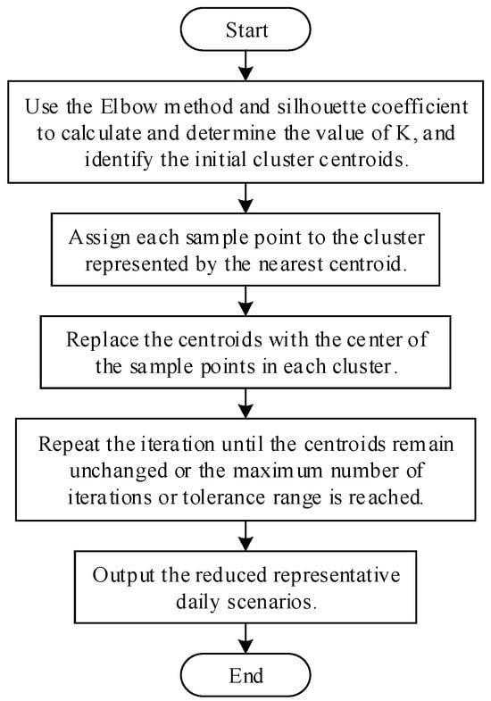
Figure 3. Scene reduction process diagram.

3. Source–Network–Storage Collaborative Planning Model Based on Stochastic Scenarios

3.1. Objective Function

The source–network–storage collaborative planning model, developed in this paper, primarily considers three types of investment costs: PV curtailment penalty costs, grid expansion investment costs, and ESS investment costs. These three aspects are used to construct the objective function for minimizing the annual distribution network comprehensive cost:

$$\min \hspace{1em}{C}_{\mathrm{inv}}={\displaystyle \sum (C_{\mathrm{Line}}+C_{\mathrm{ESS}}+C_{\mathrm{PV}})}$$

(9)

$$\left\{\begin{array}{l}{C}_{\mathrm{PV}}=365{\displaystyle \sum _{s\in {\Omega }_{\mathrm{S}}}{\displaystyle \sum _{t=1}^T{\displaystyle \sum _{i\in {\Omega }_{\mathrm{PV}}}{c}^{\mathrm{PV}}{x}_{i,s}^{\mathrm{PV}}\delta (s)(\overline{P_{i,t,s}^{\mathrm{PV}}}-P_{i,t,s}^{\mathrm{PV}})}}}\\ C_{\mathrm{Line}}={\displaystyle \sum _{s\in {\Omega }_{\mathrm{S}}}{\displaystyle \sum _{ij\in {\Omega }_{\mathrm{L}}}{x}_{ij,s}^{\mathrm{L}}{c}^{\mathrm{line}}{L}_{ij}^{\mathrm{length}}}}\\ C_{\mathrm{ESS}}={\displaystyle \sum _{s\in {\Omega }_{\mathrm{S}}}{\displaystyle \sum _{i\in {\Omega }_{\mathrm{ESS}}}{x}_{i,s}^{\mathrm{ESS}}\delta (s)(c_i^{\mathrm{e}}{E}_{i,s}^{\mathrm{e}}+c_i^{\mathrm{p}}{P}_{i,s}^{\mathrm{e}})}}\end{array}\right.$$

(10)

where $C_{\mathrm{inv}}$ represents the annual distribution network comprehensive cost; $C_{\mathrm{PV}}$ represents the annualized PV curtailment penalty cost; $C_{\mathrm{Line}}$ represents the grid expansion investment cost; $C_{\mathrm{ESS}}$ represents the annualized ESS investment/operation and maintenance cost; $c^{\mathrm{PV}}$ represents the PV curtailment penalty cost coefficient; $x_{i,s}^{\mathrm{PV}}$ is a binary decision variable, where $x_{i,s}^{\mathrm{PV}}$ = 1 if PV is installed at node i, and $x_{i,s}^{\mathrm{PV}}$ = 0 otherwise; $\delta \left(s\right)$ represents the probability of the typical scenario; $\overline{P_{i,t,s}^{\mathrm{PV}}}$ represents the predicted power output of the PV connected to node i at time t in scenario s; $P_{i,t,s}^{\mathrm{PV}}$ represents the active power output of the PV connected to node i at time t in scenario s; $x_{ij,s}^{\mathrm{L}}$ is a binary decision variable, where $x_{ij,s}^{\mathrm{L}}$ = 1 if node i is connected to node j, and $x_{ij,s}^{\mathrm{L}}$ = 0 otherwise; $c^{\mathrm{line}}$ represents the cost per unit length for building the transmission line, and $L_{ij}^{\mathrm{length}}$ represents the length of the transmission line; $x_{i,s}^{\mathrm{ESS}}$ is a binary decision variable, where $x_{i,s}^{\mathrm{ESS}}$ = 1 if ESS is installed at node i, and $x_{i,s}^{\mathrm{ESS}}$ = 0 otherwise; $c_i^{\mathrm{e}}$ and $c_i^{\mathrm{p}}$ represent the unit capacity investment/operation and maintenance costs for ESS at node i and the unit power investment/operation and maintenance costs, respectively; $E_{i,s}^{\mathrm{e}}$ represents the rated capacity of the ESS; $P_{i,s}^{\mathrm{e}}$ represents the rated power of the ESS; ${\Omega }_{\mathrm{S}}$ represents the set of scenarios; ${\Omega }_{PV}$ represents the set of candidate PV connection nodes; ${\Omega }_{\mathrm{L}}$ represents the set of distribution network grid lines; and ${\Omega }_{ESS}$ represents the set of candidate ESS connection nodes.

3.2. Constraints

3.2.1. Constraints of Distributed PV

The increase in PV capacity will lead to overvoltage issues in the grid. To address this problem, this paper adopts the Optimal Inverter Dispatch [28] (OID) strategy, which controls the active and reactive power of PV simultaneously. The operating range of PV under the OID strategy is illustrated in Figure 4.

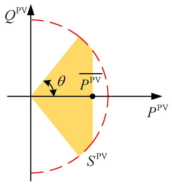
Figure 4. PV operating area under the OID strategy.

• Constraints of Operation

$$\left\{\begin{array}{l}0\le P_{i,t,s}^{\mathrm{PV},\mathrm{x}}\le \overline{P_{i,t,s}^{\mathrm{PV}}}\\ {(P_{i,t,s}^{\mathrm{PV},\mathrm{x}})}^2+{(Q_{i,t,s}^{\mathrm{PV},\mathrm{x}})}^2\le {(S_{i,t,s}^{\mathrm{PV}})}^2\\ -P_{i,t,s}^{\mathrm{PV},\mathrm{x}}\tan {\theta }_i\le Q_{i,t,s}^{\mathrm{PV},\mathrm{x}}\le P_{i,t,s}^{\mathrm{PV},\mathrm{x}}\tan {\theta }_i\\ -M\times x_{i,s}^{\mathrm{PV}}\le P_{i,t,s}^{\mathrm{PV},\mathrm{x}}\le M\times x_{i,s}^{\mathrm{PV}}\\ P_{i,t,s}^{\mathrm{PV}}-M\times (1-x_{i,s}^{\mathrm{PV}})\le P_{i,t,s}^{\mathrm{PV},\mathrm{x}}\le P_{i,t,s}^{\mathrm{PV}}+M\times (1-x_{i,s}^{\mathrm{PV}})\end{array}\right.$$

(11)

where $Q_{i,t,s}^{\mathrm{PV}}$ represents the reactive power of the PV connected to node i at time t in scenario s; $S_{i,t,s}^{\mathrm{PV}}$ represents the rated capacity of the PV connected to node i at time t in scenario s; ${\theta }_i$ represents the power factor angle of the PV; $P_{i,t,s}^{\mathrm{PV},\mathrm{x}}=x_{i,s}^{\mathrm{PV}}{P}_{i,t,s}^{\mathrm{PV}}$ and $Q_{i,t,s}^{\mathrm{PV},\mathrm{x}}=x_{i,s}^{\mathrm{PV}}{Q}_{i,t,s}^{\mathrm{PV}}$ are intermediate auxiliary variables. M represents a sufficiently large positive number.

• Constraints of Nominal Capacity

$$0\le S_{i,t,s}^{\mathrm{PV}}\le S_{i,\max }^{\mathrm{PV}}$$

(12)

where $S_{i,\max }^{\mathrm{PV}}$ represents the maximum capacity of PV that can be installed at node i.

• Constraints of the Number of PV

$${\displaystyle \sum _{i=1}^{N_L}{x}_{i,s}^{\mathrm{PV}}}\le N_{\mathrm{PV}}$$

(13)

where $N_{\mathrm{L}}$ represents the number of nodes, and $N_{\mathrm{PV}}$ represents the maximum number of PV installations allowed in the distribution network.

3.2.2. Constraints of ESS

Given that the changes in PV output do not exactly match the changes in load demand, PV can only adopt the curtailment strategy to satisfy the above stringent constraints based on substation power, node voltage, and branch current limits in the distribution network. The source–network–storage collaborative planning method proposed in this paper makes full use of the PV in the distribution network by introducing ESS to smooth voltage fluctuation and improves the capacity of the distribution network to consume PV generation.

• Constraints of Operation

$$\left\{\begin{array}{l}{u}_{i,t,s}^{\mathrm{ch}}+u_{i,t,s}^{\mathrm{dis}}\le x_{i,s}^{\mathrm{ESS}}\\ 0\le P_{i,t,s}^{\mathrm{ch}}\le P_{i,s}^{\mathrm{e},\mathrm{ch}}\\ 0\le P_{i,t,s}^{\mathrm{dis}}\le P_{i,s}^{\mathrm{e},\mathrm{dis}}\\ E_{i,t,s}=E_{i,t-1,s}+(P_{i,t,s}^{\mathrm{ch}}{\eta }_{\mathrm{ch},i}-{\displaystyle \frac{P_{i,t,s}^{\mathrm{dis}}}{{\eta }_{\mathrm{dis},i}}})\Delta t\\ 0.2E_{i,s}^{\mathrm{e},\mathrm{x}}\le E_{i,t,s}\le \hspace{0.33em}0.9E_{i,s}^{\mathrm{e},\mathrm{x}}\\ -M\times u_{i,t,s}^{\mathrm{ch}}\le P_{i,s}^{\mathrm{e},\mathrm{ch}}\le M\times u_{i,t,s}^{\mathrm{ch}}\\ P_{i,s}^{\mathrm{e}}-M\times (1-u_{i,t,s}^{\mathrm{ch}})\le P_{i,s}^{\mathrm{e},\mathrm{ch}}\le P_{i,s}^{\mathrm{e}}+M\times (1-u_{i,t,s}^{\mathrm{ch}})\\ -M\times u_{i,t,s}^{\mathrm{dis}}\le P_{i,s}^{\mathrm{e},\mathrm{dis}}\le M\times u_{i,t,s}^{\mathrm{dis}}\\ P_{i,s}^{\mathrm{e}}-M\times (1-u_{i,t,s}^{\mathrm{dis}})\le P_{i,s}^{\mathrm{e},\mathrm{dis}}\le P_{i,s}^{\mathrm{e}}+M\times (1-u_{i,t,s}^{\mathrm{dis}})\\ -M\times x_{i,s}^{\mathrm{ESS}}\le E_{i,s}^{\mathrm{e},\mathrm{x}}\le M\times x_{i,s}^{\mathrm{ESS}}\\ E_{i,s}^{\mathrm{e}}-M\times (1-x_{i,s}^{\mathrm{ESS}})\le E_{i,s}^{\mathrm{e},\mathrm{x}}\le E_{i,s}^{\mathrm{e}}+M\times (1-x_{i,s}^{\mathrm{ESS}})\end{array}\right.$$

(14)

where $u_{i,t,s}^{\mathrm{ch}}$ and $u_{i,t,s}^{\mathrm{dis}}$ are binary decision variables, representing the two states of ESS: charging state and discharging state, respectively; $P_{i,t,s}^{\mathrm{ch}}$ and $P_{i,t,s}^{\mathrm{dis}}$ represent the charging power and discharging power of the ESS, respectively; $E_{i,t,s}$ represents the energy stored in the ESS at node i at time t; ${\eta }_{\mathrm{ch},i}$ represents the charging efficiency of the ESS at node i; ${\eta }_{\mathrm{dis},i}$ represents the discharging efficiency of the ESS at node i; $\Delta t$ represents the scheduling time interval of the ESS; $P_{i,s}^{\mathrm{e},\mathrm{ch}}=u_{i,t,s}^{\mathrm{ch}}{P}_{i,s}^{\mathrm{e}}$, $P_{i,s}^{\mathrm{e},\mathrm{dis}}=u_{i,t,s}^{\mathrm{dis}}{P}_{i,s}^{\mathrm{e}}$, and $E_{i,s}^{\mathrm{e},\mathrm{x}}=x_{i,s}^{\mathrm{ESS}}{E}_{i,s}^{\mathrm{e}}$ represent intermediate auxiliary variables.

• Constraints of the Rated Power

$$x_{i,s}^{\mathrm{ESS}}{P}_{i,\min }^{\mathrm{e}}\le P_{i,s}^{\mathrm{e}}\le x_{i,s}^{\mathrm{ESS}}{P}_{i,\max }^{\mathrm{e}}$$

(15)

where $P_{i,\min }^{\mathrm{e}}$ and $P_{i,\max }^{\mathrm{e}}$ represent the lower and upper limits of the rated power of the ESS, respectively.

• Constraints of the Rated Capacity

$$0\le E_{i,s}^{\mathrm{e}}\le x_{i,s}^{\mathrm{ESS}}{E}_{i,\max }^{\mathrm{e}}$$

(16)

where $E_{i,\max }^{\mathrm{e}}$ represents the upper limit of the rated capacity of the ESS.

• Constraints of the Number of ESS

$${\displaystyle \sum _{i=1}^{N_{\mathrm{L}}}{x}_{i,s}^{\mathrm{ESS}}}\le N_{\mathrm{ESS}}$$

(17)

where $N_{\mathrm{ESS}}$ represents the maximum number of ESS installations allowed in the distribution network.

3.2.3. Constraints of Grid Expansion

This section adopts a radial topology. Considering single-commodity flow constraints (SCF) [29] and the quantitative relationship between nodes and edges, the distribution network expansion model is constructed. The single-commodity flow constraints ensure the connectivity of the graph in the form of virtual flows.

• Single-Commodity Flow Constraints

$$\left\{\begin{array}{l}{\displaystyle \sum _{(ji)\in {\Omega }_{\mathrm{L}}}{F}_{ji,t,s}}-{\displaystyle \sum _{(ij)\in {\Omega }_{\mathrm{L}}}{F}_{ij,t,s}}=1\hspace{1em}\forall i\in N_{\mathrm{L}}\backslash R\\ -M(x_{ij,s}^{\mathrm{L}}+x_{ij}^0)\le F_{ij,t,s}\le M(x_{ij,s}^{\mathrm{L}}+x_{ij}^0)\end{array}\right.$$

(18)

where $F_{ji,t,s}$ and $F_{ij,t,s}$ represent the virtual power flowing from node j to node i and from node i to node j at time t in scenario s, respectively; 1 represents the virtual load at a regular node; $x_{ij}^0$ is an undirected binary integer constant, indicating whether an initial transmission line has been constructed between node i and j. If such a line exists, $x_{ij}^0$ = 1; otherwise, $x_{ij}^0$ = 0. R represents the number of substation nodes.

• Constraints of the Quantitative Relationship Between Nodes and Edges

$${\displaystyle \sum _{(ij)\in {\Omega }_{\mathrm{L}}}(x_{ij}^0+x_{ij,s}^{\mathrm{L}})}=\left|N_{\mathrm{L}}\right|-\left|R\right|$$

(19)

• Constraints of Grid Expansion

$$x_{ij,s}^{\mathrm{L}}+x_{ij}^0\le 1$$

(20)

3.2.4. Constraints of Power Flow

Considering the addition of grid expansion constraints, constraints on the branch circuit power need to be included. This paper adopts second-order cone relaxation (SOCR) [30,31] to convexly relax the power flow equations. The transformed mixed-integer second-order cone programming (MISOCP) power flow model is as follows:

• Power Flow Model

$$\left\{\begin{array}{l}{p}_{i,t,s}={\displaystyle \sum _{k:j\to k}{P}_{jk,t,s}}-{\displaystyle \sum _{i:i\to j}(P_{ij,t,s}-r_{ij}{l}_{ij,t,s})}\\ q_{i,t,s}={\displaystyle \sum _{k:j\to k}{Q}_{jk,t,s}}-{\displaystyle \sum _{i:i\to j}(Q_{ij,t,s}-x_{ij}{l}_{ij,t,s})}\\ \left|\begin{array}{l}{v}_{i,t,s}-v_{j,t,s}-2(r_{ij}{P}_{ij,t,s}+x_{ij}{Q}_{ij,t,s})\\ +(r_{ij}^2+x_{ij}^2)l_{ij,t,s}(x_{ij,s}^{\mathrm{L}}+x_{ij}^0)\end{array}\right|\le M(1-x_{ij,s}^{\mathrm{L}}-x_{ij}^0)\\ {‖\begin{array}{c}2P_{ij,t}\\ 2Q_{ij,t}\\ l_{ij,t}-V_{i,t}\end{array}‖}_2\le l_{ij,t}+V_{i,t}\end{array}\right.$$

(21)

where $p_{i,t,s}$ and $q_{i,t,s}$ represent the active and reactive power injections at node j at time t in scenario s, respectively; $P_{jk,t,s}$ and $Q_{jk,t,s}$ represent the active and reactive power flows out of node j at time t in scenario s, respectively; $P_{ij,t,s}$ and $Q_{ij,t,s}$ represent the active and reactive power flowing into node j at time t in scenario s, respectively; $r_{ij}$ and $x_{ij}$ represent the resistance and reactance on branch ij; $l_{ij,t,s}$ represents the square of the current on branch ij at time t in scenario s; $v_{i,t,s}$ and $v_{j,t,s}$ represent the square of the voltage at node i and j at time t in scenario s, respectively; $l_{ij,t}$ represents the square of the current on branch ij at time t, and $l_{ij,t}={\left|I_{ij}\right|}^2$; $V_{i,t}$ represents the square of the voltage at node i at time t, and $V_{i,t}={\left|U_i\right|}^2$.

• Constraints of the Voltage

$$\underset{¯}{v_i}\le v_{i,t,s}\le \overline{v_i}$$

(22)

where $\underset{¯}{v_i}$ and $\overline{v_i}$ represent the upper and lower limits of the square of the voltage at node i, respectively.

• Constraints of the Current

$$0⩽l_{ij,t,s}⩽(x_{ij,s}^{\mathrm{L}}+x_{ij}^0)\overline{l_{ij}}$$

(23)

where $\overline{l_{ij}}$ represents the upper limit of the square of the current on branch ij.

• Constraints of the Power

$$\left\{\begin{array}{l}\underset{¯}{p_i}\le p_{i,t,s}\le \overline{p_i}\\ \underset{¯}{q_i}\le q_{i,t,s}\le \overline{q_i},\end{array}\right.$$

(24)

where $\underset{¯}{p_i}$ and $\overline{p_i}$ represent the minimum and maximum active power of the substation generator at node i, respectively; $\underset{¯}{q_i}$ and $\overline{q_i}$ represent the minimum and maximum reactive power of the substation generator at node i, respectively.

• Constraints of the Branch Circuit Power

$$\left\{\begin{array}{l}-(x_{ij,s}^{\mathrm{L}}+x_{ij}^0)P_{ij}^{\max }⩽P_{ij,t,s}⩽(x_{ij,s}^{\mathrm{L}}+x_{ij}^0)P_{ij}^{\max }\\ -(x_{ij,s}^{\mathrm{L}}+x_{ij}^0)Q_{ij}^{\max }⩽Q_{ij,t,s}⩽(x_{ij,s}^{\mathrm{L}}+x_{ij}^0)Q_{ij}^{\max }\end{array}\right.$$

(25)

where $P_{ij}^{\max }$ and $Q_{ij}^{\max }$ represent the maximum values of active power and reactive power on branch ij, respectively.

3.2.5. Constraints of Other Equipment

With the increasing penetration of PV, the current reversal may occur in the distribution network during off-peak hours. This problem can be mitigated by installing reactive power compensation devices in the distribution network. If voltage problems arise due to the high proportion of PV generation, an on-load tap changer (OLTC) can be equipped in the distribution network to stabilize its operation [32].

• Constraints on the Operation of Group-Cutting Capacitors (CBs)

$$\left\{\begin{array}{l}{Q}_{i,t,s}^{\mathrm{CB}}=n_{i,t,s}^{\mathrm{CB}}{q}_i^{CB}\\ 0\le n_{i,t,s}^{\mathrm{CB}}\le N_i^{\mathrm{CB}}\\ {\displaystyle \sum _{t=1}^{T-1}{B}_{i,\mathrm{CB}}^t}=B_{\mathrm{CB}}^{\lim }\end{array}\right.,n_{i,t,s}^{\mathrm{CB}}\in {\mathrm{Z}}^{+}$$

(26)

where $Q_{i,t,s}^{\mathrm{CB}}$ represents the actual compensation power delivered by the CB at node i at time t in scenario s; $n_{i,t,s}^{\mathrm{CB}}$ represents the number of CB units in operation at node i at time t in scenario s; $q_i^{\mathrm{CB}}$ represents the compensation power of a single CB unit; $N_i^{CB}$ represents the maximum number of CB units at node i; $B_{\mathrm{CB}}^{\lim }$ represents the action frequency limit of the CB units within T scheduling periods in a day; $B_{i,\mathrm{CB}}^t$ is a 0–1 integer variable representing the decision: if the CB is operated, $B_{i,\mathrm{CB}}^t$ = 1; otherwise, $B_{i,\mathrm{CB}}^t$ = 0.

• Constraints on the Operation of Static Var Compensation (SVC)

$$Q_{i,\min }^{\mathrm{SVC}}\le Q_{i,t,s}^{\mathrm{SVC}}\le Q_{i,\max }^{\mathrm{SVC}}$$

(27)

where $Q_{i,t,s}^{\mathrm{SVC}}$ represents the optimized reactive power adjustment for each phase of the SVC connected at node i at time t in scenario s; $Q_{i,\min }^{\mathrm{SVC}}$ and $Q_{i,\max }^{\mathrm{SVC}}$ represent the lower and upper limits of the adjustable reactive power for each phase of the SVC, respectively.

• Constraints on the Operation of the On-load Tap Changer (OLTC)

Figure 5 shows the branch model with an OLTC. The constraints on the operation of the OLTC are as follows:

$$\left\{\begin{array}{l}{m}_{ij,t,s}=k_{ij}^{\min }{v}_{j,t,s}+\Delta k_{ij,t,s}{\displaystyle \sum _{n=0}^{K_{ij}}{2}^n{x}_{ij,n,t}}\\ 0\le v_{j,t,s}-x_{ij,n,t}\le (1-{\lambda }_{ij,n,t})M\\ 0\le x_{ij,n,t}\le {\lambda }_{ij,n,t}M\\ v_{o,t,s}=k_{ij}^{\min }{m}_{ij,t,s}+\Delta k_{ij,t,s}{\displaystyle \sum _{n=0}^{N_{ij}}{2}^n{y}_{ij,n,t}}\\ 0\le m_{ij,t,s}-y_{ij,n,t}\le (1-{\lambda }_{ij,n,t})M\\ 0\le y_{ij,n,t}\le {\lambda }_{ij,n,t}M\\ {\displaystyle \sum _{n=0}^{N_{ij}}{2}^n{\lambda }_{ij,n,t}}\le K_{ij}\end{array}\right.$$

(28)

where $v_{o,t,s}$ represents the square of the voltage at node i at time t; $N_{ij,t,s}$ represents the tap position of the OLTC installed on branch ij at time t in scenario s; $k_{ij,t,s}$ represents the transformation ratio of the OLTC installed on branch ij at time t in scenario s; $\Delta k_{ij}$ represents the unit adjustment step of the OLTC; $K_{ij}$ represents the number of tap positions of the OLTC; $k_{ij}^{\max }$ and $k_{ij}^{\min }$ represent the amplitude of the transformation ratio of the OLTC on branch ij; $x_{ij,n,t}={\lambda }_{ij,n,t}{v}_{j,t,s}$ and $y_{ij,n,t}={\lambda }_{ij,n,t}{m}_{ij,t,s}$ are auxiliary variables; and ${\lambda }_{ij,n,t}$ represents the combination of {0,1}.

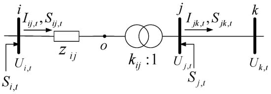
Figure 5. Branch model with the OLTC.

4. Case Study

4.1. System Setup for the Case Study

To verify the effectiveness of the proposed source–network–storage collaborative planning method based on stochastic scenarios for improving the efficient utilization of PV and the economic planning of the distribution network, this paper uses the 25-bus system and 54-bus system shown in Figure 6 and Figure 7 as models and uses YALMIP and the solver GUROBI to solve the problem. The planning results for the distribution network under different scenarios are solved on a personal computer with an Intel Core(^TM) i5-11320H CPU, 3.20 GHz, using MATLAB R2020b. As shown in Table 1, four schemes are set up:

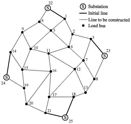
Figure 6. 25-bus system.

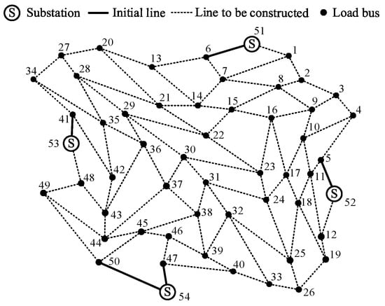
Figure 7. The 54-bus system.

Table 1. Scheme settings.

Scheme	Grid Expansion	PV Siting and Capacity Setting	ESS Siting and Capacity Setting	Reactive Power Compensation	OLTC
1	√	—	—	—	—
2	√	√	—	√	√
3	√	—	√	√	√
4	√	√	√	√	√

Scheme 1: Only considers grid expansion.

Scheme 2: Consider grid expansion, PV siting and capacity setting, OLTC adjustment, and reactive power compensation.

Scheme 3: Consider grid expansion, ESS siting and capacity setting, OLTC adjustment, and reactive power compensation.

Scheme 4: Consider grid expansion, PV siting and capacity setting, ESS siting and capacity setting, OLTC adjustment, and reactive power compensation.

The system parameters and equipment parameters for the case study are provided in Table 2, Table 3, Table 4, Table 5, Table 6, Table 7 and Table 8.

Table 2. System parameter information.

Parameter	25-Bus System	54-Bus System
Substation active power/kW	[0, 5000]	[0, 10,000]
Substation reactive power/kW	[0, 2500]	[0, 5000]
Limit of bus voltage/p.u.	[0.95, 1.05]	[0.95, 1.05]
Upper limit of branch power/MVA	10	10
Upper limit of branch current/p.u.	1	1
Reference voltage/kV	12.66	12.66
Reference power/MW	10	10

Table 3. PV parameter information.

Limitations of PV	25-Bus System	54-Bus System
Installation quantity limit in Scheme 1	0	0
Installation quantity limit in Scheme 2	[2, 5]	[3, 8]
Installation quantity limit in Scheme 3	0	0
Installation quantity limit in Scheme 4	[3, 8]	[5, 10]
Maximum installation capacity at buses/MW	1.5	3

Table 4. ESS parameter information.

Limitations of ESS	25-Bus System	54-Bus System
Installation quantity limit in Scheme 1	0	0
Installation quantity limit in Scheme 2	0	0
Installation quantity limit in Scheme 3	[1, 5]	[1, 8]
Installation quantity limit in Scheme 4	[1, 5]	[1, 8]
Rated power/MW	2	2
Charging efficiency	0.9	0.9
Discharging efficiency	1	1
Limit of SOC	[0.2, 0.9]	[0.2, 0.9]

Table 5. CB parameter information.

Limitations of CB	25-Bus System	54-Bus System
Buses to be installed in Scheme 1	—	—
Buses to be installed in Scheme 2	21	13
Buses to be installed in Scheme 3	21	13
Buses to be installed in Scheme 4	21	13
Reactive power per compensation unit/kVar	50	50
Maximum number of compensation units	4	4
Maximum number of CB operations per day	5	5

Table 6. SVC parameter information.

Limitations of SVC	25-Bus System	54-Bus System
Buses to be installed in Scheme 1	—	—
Buses to be installed in Scheme 2	18	6
Buses to be installed in Scheme 3	18	6
Buses to be installed in Scheme 4	18	6
Compensation range/kVar	[−200, 300]	[−200, 300]

Table 7. OLTC parameter information.

Limitations of OLTC	25-Bus System	54-Bus System
Branches to be installed in Scheme 1	—	—
Branches to be installed in Scheme 2	1–22, 3–23, 14–24, 21–25	5–52, 6–51, 41–53, 50–54
Branches to be installed in Scheme 3	1–22, 3–23, 14–24, 21–25	5–52, 6–51, 41–53, 50–54
Branches to be installed in Scheme 4	1–22, 3–23, 14–24, 21–25	5–52, 6–51, 41–53, 50–54
Transformer ratio	[0.95, 1.05]	[0.95, 1.05]
Tap change step value of the transformer	0.01	0.01
Number of taps on the transformer	10	10

Table 8. Cost information.

Costs	Value
PV curtailment penalty/(CNY/kWh)	3.6
Annualized investment cost per unit capacity of ESS/(CNY/kWh)	1270
Annualized investment cost per unit power of ESS/(CNY/kWh)	1650
Unit length construction cost of the line/(CNY10,000/km)	36.2

To evaluate the power supply reliability of the planning scheme, this study introduces the Expected Energy Not Supplied (EENS) as an evaluation metric. EENS refers to the amount of energy that cannot be delivered to users due to insufficient supply capacity over a given period. It is calculated using the following formula:

$$EENS=365{\displaystyle \sum _{s\in {\Omega }_{\mathrm{S}}}{\displaystyle \sum _{t=1}^T{\displaystyle \sum _{i\in \Omega }\delta (s){(P_{i,t,s}^{\mathrm{Load}}-P_{i,t,s}^{\mathrm{Sup}})}^{+}}}}\times \Delta t$$

(29)

$$P_{i,t,s}^{\mathrm{Sup}}=P_{i,t,s}^{\mathrm{PV}}+P_{i,t,s}^{\mathrm{Line}}+P_{i,t,s}^{\mathrm{dis}}-P_{i,t,s}^{\mathrm{ch}}$$

(30)

where $P_{i,t,s}^{\mathrm{Load}}$ represents the load power of node i at time t in scenario s; $P_{i,t,s}^{\mathrm{Sup}}$ represents the supplied power of node i at time t in scenario s; $P_{i,t,s}^{\mathrm{Line}}$ represents the transmission power of lines connected to node i at time t in scenario s; ${(\cdot )}^{+}$ represents taking the positive part (i.e., the value is counted only when the load exceeds the supplied power); Ω represents the set of all nodes; $\Delta t$ represents the time step.

4.2. Analysis of Stochastic Scenarios

The goodness of fit of different Copula functions was evaluated using the correlation coefficient method and the Euclidean distance method. The most suitable Copula function was selected based on these results, as shown in Table 9.

Table 9. Fit degree discrimination of different functions.

	Normal Copula	t-Copula	Gumbel Copula	Clayton Copula	Frank Copula	Sample Data
Kendall rank correlation coefficient	−0.078	−0.091	1.457 × 10−6	7.729 × 10−7	−0.089	−0.082
Spearman rank correlation coefficient	−0.087	−0.133	2.936 × 10−6	1.169 × 10−6	−0.127	−0.122
Squared Euclidean distance	0.842	107.173	2.169	2.749	0.226	0

As shown in Table 9, compared to other methods, the correlation coefficient obtained by the Frank Copula method has a better fit with the sample data and a smaller Euclidean distance to the empirical Copula. Although the correlation coefficient of t-Copula is acceptable, its Euclidean distance to the empirical Copula is large, indicating that its fitting performance is not ideal. Therefore, t-Copula is not suitable as the optimal fitting function. After comprehensive consideration, Frank Copula is selected for data fitting in this paper to ensure the accuracy and reliability of the fitting results.

The Monte Carlo method is used to perform random sampling for each time period in the source load temporal–spatial correlation probabilistic model based on Copula theory. In this process, the number of load and PV output scenarios is set to 3650 to ensure the randomness and diversity of the scenarios. Through this method, a large number of source load temporal–spatial correlation scenarios are generated, as shown in Figure 8.

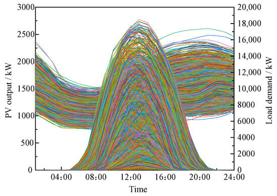
Figure 8. Scene generation.

To ensure computational accuracy while maximizing efficiency, the K-means clustering algorithm is employed to reduce the 3650 source load temporal–spatial correlation scenarios. The clustering algorithm is based on the computation of the sum of squared errors (SSE), silhouette efficiency (SE), and the similarity coefficient between scenarios. The optimal number of clusters is defined as the number of clusters where the SSE is small and the SE is large. The number of clusters is varied from 1 to 15, and the SSE and SC indices for each cluster are calculated and plotted as curves. By examining the SSE and SC curves, the appropriate number of clusters is determined to be four. The 3650 scenarios are then divided into four clusters, resulting in four typical source load temporal–spatial correlation scenarios. The algorithm process is shown in Figure 9, and the resulting output curves for the typical scenarios are shown in Figure 10. The details of each typical scenario are provided in Table 10.

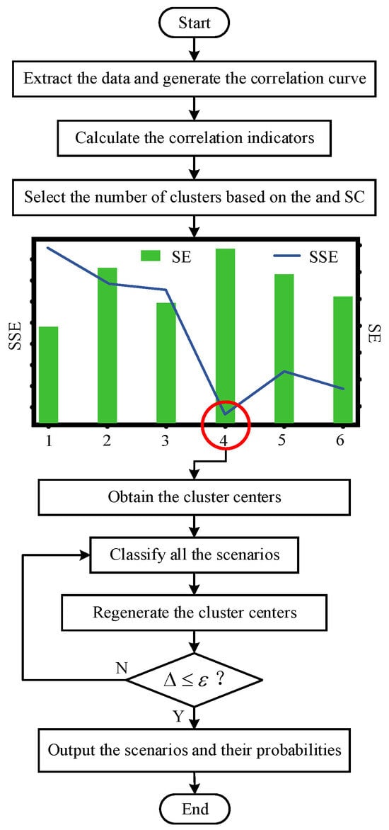
Figure 9. Typical scene generation algorithm flow.

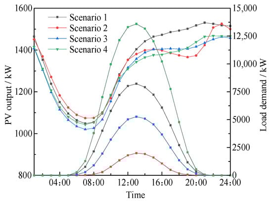
Figure 10. Typical day scenarios based on Copula theory.

Table 10. Typical scenario probability based on Copula theory.

Typical Daily Scenarios	Probability
1	0.3907
2	0.0696
3	0.2444
4	0.2953

By observing Figure 10, it can be seen that, during specific time periods, the variation trends of PV output and load in different scenarios exhibit a certain degree of correlation: they either increase or decrease simultaneously or show opposite trends. This correlation is not accidental but is due to the source load temporal–spatial correlation probability model based on Copula theory. This model effectively captures the temporal–spatial correlation between source and load outputs, thereby reducing the impact of uncertainties on the distribution network. Therefore, the source load temporal–spatial correlation scenarios generated by this model can accurately simulate the source load temporal–spatial correlation of the region, providing an important reference value for distribution network planning.

To more intuitively demonstrate this correlation, the source load output curves from Scenario 1, which has the highest probability of occurrence, are selected for comparison, as shown in Figure 11. By comparing these curves, the dynamic relationship between the source and load outputs becomes more clearly visible.

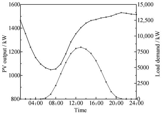
Figure 11. Source load output curve under Scenario 1.

From Figure 11, it can be observed that both the load demand curve and the PV output curve exhibit fluctuations. These fluctuations are primarily due to variations in sunlight intensity at different times of the day and people’s electricity consumption habits. Notably, PV output is almost zero at night, while, during the daytime, from sunrise to sunset, it shows higher output levels. At the same time, the load also shows a distinct upward trend after sunrise, indicating that PV generation output and load demand are positively correlated in terms of both time and space, in most cases.

Further observation of the PV output curve and the load curve reveals that, at certain times, the degree of variation for both curves is quite similar, for example, between 6 a.m. and 2 p.m. At other times, such as between 2 p.m. and 8 p.m., their variation trends are the opposite. This suggests that the relationship between PV generation output and load demand is not fixed but can show either a positive or negative correlation, depending on the specific situation. This variation closely reflects the real-world scenario, illustrating the complex relationship between load demand and PV output.

Therefore, by applying the obtained source load temporal–spatial correlation typical scenarios to the source–network–storage collaborative planning model for the distribution network, the correlation between source and load can be more accurately reflected. This model design ensures that the results are more aligned with actual operating conditions, contributing to improving the economic efficiency of distribution network planning and enhancing its operational reliability. By fully considering the temporal–spatial correlation between source and load, it becomes possible to better optimize resource allocation, improve energy utilization efficiency, and ensure that the distribution network can maintain efficient and stable operation when facing various complex scenarios.

4.3. Analysis of the 25-Bus System Planning Results

To facilitate the presentation of the results, the PV configuration, ESS configuration, and network expansion planning results in this paper are all based on Scenario 1, which has the highest probability. According to the Scenario 1 case results, the PV and ESS planning configuration results for the 25-bus system under different schemes are shown in Table 11 and Table 12, respectively. The cost comparisons under different schemes are shown in Table 13.

Table 11. PV planning and configuration results in different schemes.

System	Scheme	Installed Bus	Installed Capacity/MW	Total Generation/MWh
25-bus system	2	10, 12, 19	9.85	7019.54
	4	10, 12, 16, 19	11.82	9502.61

Table 12. ESS planning and configuration results in different schemes.

System	Scheme	Installed Bus	Total Installed Apparent Power/kVA	Total Installed Capacity/kWh
25-bus system	3	5, 16	1100	1600
	4	2, 11, 17	1700	2200

Table 13. Cost comparison of 25-bus system planning in different schemes.

	Scheme 1	Scheme 2	Scheme 3	Scheme 4
ESS investment cost/CNY10,000	0	0	227.3	343.13
Curtailment penalty cost/CNY10,000	0	1354.24	0	42.64
Grid expansion cost/CNY10,000	618.24	589.23	640.23	589.26
Distribution network comprehensive cost/CNY10,000	618.24	1943.47	867.53	975.03
EENS	0	0	0	0
Solving time/s	145.27	269.27	194.94	846.69

From Table 11, it can be observed that, compared to Scheme 2, Scheme 4 increases the installed capacity of PV by 20%, and the total PV generation in the distribution network increases by approximately 35.37%. From Table 13, it can be seen that, compared to Scheme 1, Scheme 2 and Scheme 4 result in increases of approximately 214.36% and 57.71% in the distribution network comprehensive cost, respectively, while the PV installed capacity increases by 9.85 MW and 11.82 MW, and the total generation rises from 0 to 7019.54 MWh and 9502.61 MWh. The curtailment penalty costs in Scheme 2 are higher than those in Scheme 4 due to the increase in PV grid-connected capacity without appropriate ESS deployment.

From Table 12, it can be observed that, compared to Scheme 3, the total installed apparent power of ESS in Scheme 4 increases by approximately 54.55%, and the total installed capacity increases by 37.7%. From Table 13, it can be seen that, compared to Scheme 1, Scheme 3 and Scheme 4 result in increases of approximately 40.32% and 57.71% in the distribution network comprehensive cost, respectively, while the total installed capacity of ESS increases from 0 to 1.6 MWh and 2.2 MWh. The ESS investment cost in Scheme 4 is significantly higher than in Scheme 3, which is due to the increased demand for ESS resulting from the higher PV grid-connected capacity.

Based on the network construction data obtained from the solution, combined with the above planning and configuration results, the network topology diagrams after the 25-bus system planning for different schemes can be obtained, as shown in Figure 12.

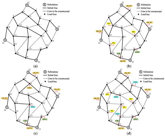
Figure 12. Planning results of the 25-bus system in different schemes. (a) Planning results of Scheme 1. (b) Planning results of Scheme 2. (c) Planning results of Scheme 3. (d) Planning results of Scheme 4.

The hourly node voltage distribution within a single day for the 25-bus system under different schemes is shown in Figure 13.

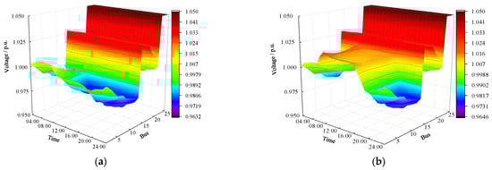
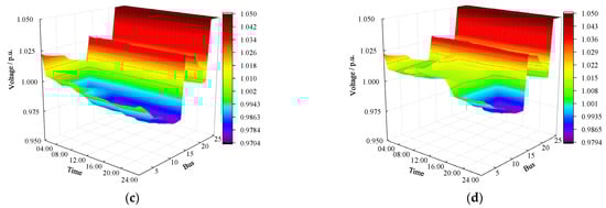
Figure 13. The 25-bus voltage distribution under Scenario 1 in different schemes. (a) Scheme 1. (b) Scheme 2. (c) Scheme 3. (d) Scheme 4.

It is evident that, although the voltage distribution in the 25-bus system under all four schemes remains within the safe range, there are noticeable differences in the distribution patterns. Compared to Scheme 1, Scheme 2 shows higher voltage fluctuations due to the integration of PV, with the voltage at the connection points being too high. In Scheme 3, the optimization of ESS configuration helps smooth the voltage fluctuations by charging during low load demand and discharging during high load demand, slightly alleviating the system’s voltage fluctuations. Scheme 4, compared to Scheme 2, adopts the “PV + ESS” collaborative planning and configuration, significantly optimizing the system’s voltage peaks and valleys by leveraging the characteristics of ESS, thereby reducing the system’s voltage fluctuation.

Based on Table 13 and Figure 14, it can be observed that the distribution network comprehensive cost of Scheme 4 is significantly lower than that of Scheme 2, with a reduction of approximately 44.88%. Although Scheme 4 increases the ESS investment cost, the “PV + ESS” collaborative planning greatly reduces the curtailment penalty costs by enhancing the distribution network’s ability to absorb PV generation, thereby improving the economic efficiency of the distribution network planning. Compared to Scheme 3, Scheme 4 increases the cost by only about 12.39% while increasing PV power generation by 9502.61 MWh, thereby enhancing the distribution network’s capacity for PV integration and power absorption. Furthermore, the calculation results of EENS show that, under all the schemes, the system is able to fully meet the load demand, and no supply shortages occur in any scenario.

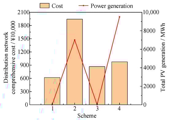
Figure 14. Distribution network comprehensive cost and total PV generation.

A comparison of the distribution network comprehensive cost, total PV installed capacity, and total PV generation before and after considering the source load correlation scenarios is shown in Table 14. After considering the source load temporal–spatial correlation scenarios, all schemes show a slight improvement compared to the schemes that do not consider these correlations. The typical daily scenarios generated using the source load temporal–spatial correlation probabilistic model based on Copula theory significantly mitigate the impact of source load uncertainty on the distribution network, enhance the network’s capacity for PV grid integration and absorption, and ultimately reduce the distribution network comprehensive cost, achieving an improvement in economic benefits.

Table 14. The system comparison before and after the source load temporal–spatial correlation scenario is considered.

Considering the Source Load Temporal–Spatial Correlation Scenario	Scheme	Distribution Network Comprehensive Cost /CNY10,000	Installed Capacity of PV/MW	Total PV Generation/MWh
Yes	1	618.24	0	0
	2	1943.47	9.85	7019.54
	3	867.53	0	0
	4	975.03	11.82	9502.61
No	1	624.25	0	0
	2	2165.97	9.06	6661.62
	3	906.87	0	0
	4	1193.95	11.397	8716.16

4.4. Analysis of the 54-Bus System Planning Results

The PV and ESS planning configuration results for the 54-bus system under different schemes are shown in Table 15 and Table 16, respectively. The cost comparison under different schemes is shown in Table 17.

Table 15. PV planning and configuration results under Scenario 1 in different schemes.

System	Scheme	Installed Bus	Installed Capacity/MW	Total Generation/MWh
54-bus system	2	22, 26, 43	17.37	14,103.26
	4	3, 25, 22, 27, 43	21.73	17,975.25

Table 16. ESS planning and configuration results under Scenario 1 in different schemes.

System	Scheme	Installed Bus	Total Installed Apparent Power/kVA	Total Installed Capacity/kWh
54-bus system	3	8, 25, 37	2000	2600
	4	8, 19, 32, 34	3200	4200

Table 17. Cost comparison of 54-bus system planning under Scenario 1 in different schemes.

	Scheme 1	Scheme 2	Scheme 3	Scheme 4
ESS investment cost/CNY10,000	0	0	354.62	478.16
Curtailment penalty cost/CNY10,000	0	2088.36	0	102.35
Grid expansion cost/CNY10,000	1375.24	1366.61	1469.27	1284.51
Distribution network comprehensive cost/CNY10,000	1375.24	3454.97	1823.89	1865.02
EENS	0	0	0	0
Solving time/s	769.20	12 146.62	1289.46	1753.08

As shown in Table 15, compared to Scheme 2, Scheme 4 increases the PV installed capacity by approximately 25.1%, and the total PV generation in the distribution network increases by about 27.45%. From Table 17, it can be seen that, compared to Scheme 1, both Scheme 2 and Scheme 4 increase the distribution network comprehensive cost by approximately 151.23% and 35.61%, respectively. However, the PV installation capacity increases by 17.37 MW and 21.73 MW, and total generation increases from 0 to 14,103.26 MWh and 17,975.25 MWh, respectively. The curtailment penalty in Scheme 2 is higher than in Scheme 4 due to the increased PV grid integration capacity without a reasonable ESS configuration.

As shown in Table 16, compared to Scheme 3, Scheme 4 increases the total installed apparent power of ESS by approximately 70.27%, and the total installed capacity increases by 64%. From Table 17, it can be seen that, compared to Scheme 1, both Scheme 3 and Scheme 4 increase the distribution network comprehensive cost by approximately 32.62% and 35.61%, respectively. Meanwhile, the total installed ESS capacity increases from 0 to 2.6 MWh and 4.2 MWh. The ESS investment cost in Scheme 4 is significantly higher than in Scheme 3, as the increased PV grid integration capacity has raised the demand for ESS.

Based on the network construction data obtained from the solution, combined with the above planning and configuration results, the network topology diagrams after the 54-bus system planning for different schemes can be obtained, as shown in Figure 15.

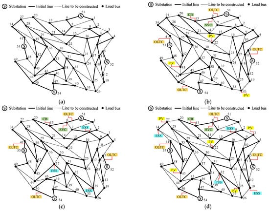
Figure 15. Planning results of the 54-bus system in different schemes. (a) Planning results of Scheme 1. (b) Planning results of Scheme 2. (c) Planning results of Scheme 3. (d) Planning results of Scheme 4.

The hourly node voltage distribution within a single day for the 54-bus system under different schemes is shown in Figure 16.

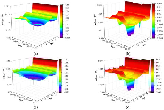
Figure 16. The 54-bus voltage distribution under Scenario 1 in different schemes. (a) Scheme 1. (b) Scheme 2. (c) Scheme 3. (d) Scheme 4.

It is evident that, although the voltage distribution in the 54-bus system under all four schemes is within the safe range, the distribution diagrams show significant differences. Compared to Scheme 1, in Scheme 2, due to the integration of PV, the voltage at the connection points becomes too high, leading to a noticeable increase in the system’s voltage volatility. Scheme 3, compared to Scheme 1, adopts an optimized ESS configuration, charging during low load demand and discharging during high load demand, thereby smoothing the peaks and valleys and slightly alleviating the system’s voltage volatility. Scheme 4, compared to Scheme 2, adopts the “PV + ESS” collaborative planning and configuration, significantly optimizing the system’s voltage peaks and valleys by leveraging the characteristics of ESS, thereby reducing the system’s voltage fluctuation.

Based on Table 17 and Figure 17, it can be observed that the distribution network comprehensive cost of Scheme 4 is significantly lower than that of Scheme 2, with a reduction of approximately 46.02%. Although Scheme 4 increases the ESS investment cost, the “PV + ESS” collaborative planning greatly reduces the curtailment penalty costs by enhancing the distribution network’s ability to absorb PV generation, thereby improving the economic efficiency of the distribution network planning. Compared to Scheme 3, Scheme 4 increases the cost by only about 2.23% while increasing PV power generation by 17,975.25 MWh, thereby enhancing the distribution network’s capacity for PV integration and power absorption. Furthermore, the calculation results of EENS show that, under all the schemes, the system is able to fully meet the load demand, and no supply shortages occur in any scenario.

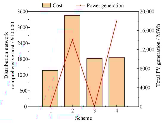
Figure 17. Distribution network comprehensive cost and total PV generation.

The comparison of the distribution network comprehensive cost, total PV installed capacity, and total PV generation before and after considering the source load correlation scenarios is shown in Table 18. After considering the source load temporal–spatial correlation scenarios, all schemes show a slight improvement compared to the schemes that do not consider these correlations. The typical daily scenarios generated using the source load temporal–spatial correlation probabilistic model based on Copula theory significantly mitigate the impact of source load uncertainty on the distribution network, enhance the network’s capacity for PV grid integration and absorption, and ultimately reduce the distribution network comprehensive cost, achieving an improvement in economic benefits.

Table 18. The system comparison before and after the source load temporal–spatial correlation scenario is considered.

Considering the Source Load Temporal–Spatial Correlation Scenarios	Scheme	Distribution Network Comprehensive Cost /CNY10,000	Installed Capacity of PV/MW	Total PV Generation/MWh
Yes	1	1375.24	0	0
	2	3454.97	17.37	14,103.26
	3	1823.89	0	0
	4	1865.02	21.73	17,975.25
No	1	1441.24	0	0
	2	3506.60	16.24	12,462.55
	3	1923.49	0	0
	4	1983.69	20.62	16,953.81

4.5. Sensitivity Analysis

4.5.1. Analysis of the Impact of PV and Load Forecasting Errors

To further evaluate the robustness of the proposed method under forecast deviations, we have extended our analysis by introducing ±10% forecast errors into both PV generation and load demand based on the four typical daily scenarios already constructed via the Copula approach (as shown in Figure 10).

Specifically, we considered two extreme error scenarios:

(1)

+10% Error Scenario (Pessimistic forecast): Actual PV output is 10% higher and load demand is 10% lower than forecasted.

(2)

−10% Error Scenario (Optimistic forecast): Actual PV output is 10% lower and load demand is 10% higher than forecasted.

Based on these two error scenarios, the source–network–storage collaborative planning under the Scheme 4 setting is performed again for the 25-bus system, and the planning results are compared with the planning results of the original scenario that do not take the prediction errors into account, and the results are shown in Table 19.

Table 19. Planning and configuration results considering forecasting errors.

	Indicator	Original Scenario	+10% Error Scenario	−10% Error Scenario
PV	Installed bus	10, 12, 16, 19	10, 12, 16, 19	10, 12, 16, 19
	Installed capacity/MW	11.82	12.15	11.60
	Total generation/MWh	9502.61	10,570.3	8510.2
ESS	Installed bus	2, 11, 17	2, 11, 17	2, 11, 17
	Total installed apparent power/kVA	1700	1780	1620
	Total installed capacity/kWh	2200	2350	2050
Cost comparison	ESS investment cost/CNY10,000	343.13	365.8	320.5
	Curtailment penalty cost/CNY10,000	42.64	65.3	28.5
	Grid expansion cost/CNY10,000	589.26	598.5	580.1
	Distribution network comprehensive cost/CNY10,000	975.03	1029.60	929.10

The comparison shows that PV and ESS siting decisions remain stable, and their capacity configurations adapt flexibly based on the system operation conditions under each error scenario. In the +10% error case, increased PV output and reduced load demand lead to more PV curtailment risk, prompting the model to increase the ESS capacity to absorb excess energy. This results in a rise in total system cost from 9.75 million CNY to 10.30 million CNY.

Conversely, in the −10% error case, a higher load and lower PV output allow the more direct consumption of PV energy, reducing the need for ESS. The system cost accordingly decreases to 9.29 million CNY due to a lower curtailment penalty and ESS investment.

These results demonstrate that the proposed planning method can adaptively adjust to forecast uncertainties while maintaining planning stability, especially in siting decisions. The model effectively mitigates the impact of forecast errors without causing disruptive changes to the overall planning scheme.

4.5.2. Comparative Analysis of Different Scenario Reduction Methods

To verify the rationality and effectiveness of the K-means clustering algorithm adopted in this study for scenario reduction, this section selects the typical simultaneous backward reduction (SBR) method as a benchmark for comparison. A comparative analysis is conducted in terms of computational efficiency and comprehensive cost, with the results summarized in Table 20.

Table 20. Performance comparison between K-means and SBR.

Method	Scenario Reduction Computation Time/s	Comprehensive Cost of 25-Bus System/CNY10,000	Comprehensive Cost of 54-Bus System/CNY10,000
K-means	6.5	975.03	1865.02
SBR	362.3	942.65	1808.70

As shown in Table 20, in terms of scenario reduction computation time, the K-means method requires only 8.5 s, whereas the SBR method takes as long as 362.3 s. This indicates that K-means significantly outperforms SBR in computational efficiency. The results clearly demonstrate that the K-means method has a substantial computational advantage when handling large-scale uncertain scenarios, contributing to an improved overall model-solving efficiency and scalability.

Regarding the optimization results, the comprehensive cost obtained using the K-means method is 3.44% and 3.11% higher than that of SBR in the 25-bus and 54-bus systems, respectively. Although there is a certain degree of cost deviation, the differences are relatively small and fall within an acceptable range in practical engineering applications. This indicates that, while significantly enhancing the reduction efficiency, the K-means method still retains the statistical characteristics of the original scenarios to a reasonable extent.

Therefore, considering both computational efficiency and the quality of the planning results, the adoption of the K-means clustering algorithm as the scenario reduction method in this study represents a well-balanced and rational choice between solution accuracy and computational feasibility. This method not only ensures that the planning outcomes remain of high reference value but also greatly improves the solution efficiency, meeting the practical needs of planning tasks.

4.5.3. Analysis of the Impact of Cost Coefficients

To further investigate the impact of key economic parameters on planning decisions, this section conducts a sensitivity analysis on several core cost coefficients, including the investment cost of ESS, the PV curtailment penalty, and the unit length construction cost of the line. By examining how variations in these coefficients influence the PV and ESS configuration, curtailment penalty cost, grid expansion, and system comprehensive cost in Scheme 4 of the 25-bus system, the trade-offs in planning strategies under different economic constraints are analyzed. The results are presented in Table 21, Table 22 and Table 23.

Table 21. Impact of ESS investment cost variations on key planning indicators.

Variation in ESS Investment Cost	Installed Capacity of PV/MW	Total Installed Capacity of ESS/kWh	Curtailment Penalty Cost/CNY10,000	Grid Expansion Cost/CNY10,000	Distribution Network Comprehensive Cost/CNY10,000
0.5	12.85	2850	20.15	575.60	791.57
0.8	12.05	2300	38.10	586.50	919.90
1.0	11.82	2200	42.64	589.26	975.03
1.2	11.75	2100	48.50	591.80	1039.00
1.5	11.25	1600	75.80	601.50	1102.95

Table 22. Impact of PV curtailment penalty variations on key planning indicators.

Variation in PV Curtailment Penalty	Installed Capacity of PV/MW	Total Installed Capacity of ESS/kWh	Curtailment Penalty Cost/CNY10,000	Grid Expansion Cost/CNY10,000	Distribution Network Comprehensive Cost/CNY10,000
0.5	12.50	2050	25.30	580.50	930.90
0.8	11.90	2180	39.10	587.80	967.10
1.0	11.82	2200	42.64	589.26	975.03
1.2	11.75	2280	48.15	592.60	996.65
1.5	11.30	2580	50.95	598.20	1047.95

Table 23. Impact of line construction cost variations on key planning indicators.

Variation in Line Construction Cost	Installed Capacity of PV/MW	Total Installed Capacity of ESS/kWh	Curtailment Penalty Cost/CNY10,000	Grid Expansion Cost/CNY10,000	Distribution Network Comprehensive Cost/CNY10,000
0.5	12.65	1950	30.50	330.15	670.85
0.8	11.90	2150	40.70	505.60	884.10
1.0	11.82	2200	42.64	589.26	975.03
1.2	11.78	2250	43.50	685.30	1079.60
1.5	11.50	2450	48.10	738.60	1168.20

Table 21 shows that the investment cost of ESS has a significant impact on the planning scheme. As the ESS investment cost decreases, the total installed capacity of ESS in the system exhibits a clear upward trend. Meanwhile, improved storage economics promote greater PV utilization, leading to an increase in the installed capacity of PV and a substantial reduction in curtailment penalty cost. Consequently, the distribution network comprehensive cost decreases significantly with the reduction in ESS costs. Conversely, when the ESS investment cost rises, the ESS capacity decreases, PV utilization is restricted, curtailment increases, and the total system cost rises.

Table 22 indicates that the PV curtailment penalty coefficient significantly affects the system’s curtailment control strategy and storage configuration. When the penalty coefficient is low, the system exhibits a higher tolerance for curtailment, possibly planning more the installed capacity of PV while allowing greater curtailment. Under this condition, the demand for ESS capacity is relatively low, and the distribution network comprehensive cost may decrease due to the reduced investment in curtailment mitigation and storage. As the penalty coefficient increases, the system strictly controls curtailment to avoid high penalties, primarily by increasing the ESS capacity. However, an excessively high penalty coefficient may lead to overinvestment in mitigation measures aimed at minimizing curtailment, thereby increasing the distribution network comprehensive cost. Therefore, setting a reasonable PV curtailment penalty coefficient is crucial to balancing PV utilization promotion and economic cost control.

Table 23 reveals that the unit length construction cost of the line directly impacts the total investment in grid expansion and indirectly influences PV and ESS configuration strategies. When the line cost is low, grid expansion becomes more economical for enabling long-distance PV transmission and utilization. Under these conditions, the system may increase the installed capacity of PV while reducing the reliance on local storage, resulting in a decreased total installed capacity of ESS. Conversely, when line construction costs are high, grid expansion becomes expensive, and the system tends to minimize reliance on line expansion by increasing the local ESS capacity or adjusting the PV layout to achieve nearby utilization. Although the physical scale of grid expansion may be constrained, the grid expansion cost still rises due to the high unit construction cost.

5. Conclusions

This paper addresses the uncertainty of PV output and load demand by establishing a source load temporal–spatial correlation probabilistic model based on Copula theory. The Monte Carlo method is used to generate numerous source load temporal–spatial correlation scenarios. Then, the K-means clustering algorithm is applied to reduce the vast scenario set, ensuring that the variability of the PV output and load demand is preserved while improving the computational efficiency, resulting in representative typical daily scenarios. On this basis, a source–network–storage collaborative planning model based on stochastic scenarios is established with the objective of minimizing the annual distribution network comprehensive cost. Through comparative analysis of case studies with 25-bus and 54-bus systems, the following conclusions are drawn:

(1)

By establishing a source load temporal–spatial correlation probabilistic model based on Copula theory and applying the Monte Carlo method and K-means clustering algorithm for scenario generation and reduction, four typical daily scenarios were obtained while preserving the variability of PV output and load demand. The results demonstrate that a small number of typical daily scenarios can effectively describe the uncertainty and temporal–spatial correlation of PV output and load demand variations while avoiding the curse of dimensionality during the solution process, further ensuring the computational efficiency.

(2)

Comparing planning schemes with and without considering source load temporal–spatial correlation, the schemes that account for this correlation consistently perform slightly better. They effectively mitigate the impact of PV and load uncertainty on the distribution network, enhance the network’s capacity for PV integration and consumption, reduce the distribution network comprehensive cost, and achieve an increase in economic benefits.

(3)

Comparing planning schemes with and without considering source load temporal–spatial correlation, the schemes that account for this correlation consistently perform slightly better. They effectively mitigate the impact of PV and load uncertainty on the distribution network, enhance the network’s PV hosting capacity, reduce the distribution network comprehensive cost, and contribute to the development of more sustainable distribution networks.

Table 24 clearly shows a comparison of the key characteristics between the method proposed in this paper and the existing research methods.

Table 24. A comparison between the method proposed in this paper and the existing research methods.

Comparison Dimension	Proposed Method in This Paper	General Characteristics of Existing Research Methods (Based on Literature Review)
Scope of planning object coordination	Source–network–storage coordinated planning: Unified optimization of PV siting and sizing, ESS siting and sizing, and distribution network expansion, pursuing system-level global optimum.	Focuses on optimizing single types of distributed resources (e.g., DG or ESS) or achieves only source-storage coordination, with insufficient consideration of the expansion and interactive effects of the distribution network, making system-level global optimization difficult.
Handling of source load temporal–spatial correlation	Explicitly models and accurately captures the complex, non-linear temporal–spatial correlation between PV output and load demand via Copula theory, significantly enhancing scenario realism and planning accuracy.	Ignores complex source load correlations or adopts simplified assumptions of independence or linear correlation, failing to accurately reflect complex interactions in real systems and leading to insufficiently refined uncertainty descriptions.
Quality of scenario generation and reduction	Generates massive annual random scenarios via Monte Carlo sampling, then efficiently reduces them using K-means clustering to obtain typical daily scenarios that reflect both annual diversity and retain key temporal characteristics.	Scenario generation methods may be simplistic (e.g., typical day method) or, while using random sampling, may not fully account for variations across different periods (e.g., inter-day), resulting in insufficient representativeness and diversity of scenarios.
Planning objective and overall benefits	Aims to enhance efficient PV accommodation and the overall economics of distribution network planning, striving to achieve dual improvements in the PV hosting capacity and economic benefits through comprehensive coordination and refined modeling.	The objective may focus on local optimization (e.g., specific equipment economics or performance indicators), or due to a lack of comprehensive coordination and refined uncertainty/correlation handling, PV hosting potential may not be fully exploited, and the overall system economics and robustness to uncertainty need improvement.

Despite the promising results achieved in this study, several directions remain open for further research and development:

(1) Multi-objective coordinated planning and Pareto analysis:

This paper promotes PV utilization indirectly by incorporating the curtailment penalty cost into the comprehensive cost function. Future work may explicitly formulate a multi-objective optimization model that simultaneously considers planning economy, system reliability, and maximization of renewable energy integration (or minimization of carbon emissions). Solving such multi-objective problems and analyzing the resulting Pareto frontier can provide decision-makers with more intuitive and informative trade-off analyses among competing objectives.

(2) Validation and extension of the proposed method to more complex and realistic distribution networks:

This study primarily uses typical radial feeders as test systems. Future research will further validate and extend the proposed method on more complex benchmark networks, such as the IEEE 123-bus system, or on real-world utility distribution feeders. The feasibility, computational performance, and planning effectiveness of the method under complex topologies will be systematically evaluated. In addition, future work will explore the relaxation accuracy of power flow modeling under non-radial structures, as well as the development of coordinated control strategies in multi-source, multi-loop distribution systems, laying a solid foundation for real-world engineering applications.

References

- Ding, T.; Li, C.; Yang, Y.; Jiang, J.; Bie, Z.; Blaabjerg, F. A Two-Stage Robust Optimization for Centralized-Optimal Dispatch of Photovoltaic Inverters in Active Distribution Networks. IEEE Trans. Sustain. Energy 2017, 8, 744–754. [Google Scholar] [CrossRef]
- Jafari, M.R.; Parniani, M.; Ravanji, M.H. Decentralized Control of OLTC and PV Inverters for Voltage Regulation in Radial Distribution Networks with High PV Penetration. IEEE Trans. Power Deliv. 2022, 37, 4827–4837. [Google Scholar] [CrossRef]
- Le, J.; Lang, H.; Liao, X.; Wang, J.; Mao, T. Affinely Adjustable Robust Optimization Method for Active Distribution Network Based on Generalized Linear Polyhedral. Autom. Electr. Power Syst. 2023, 47, 138–148. [Google Scholar]
- Ayalew, M.; Khan, B.; Giday, I.; Mahela, O.P.; Khosravy, M.; Gupta, N.; Senjyu, T. Integration of Renewable Based Distributed Generation for Distribution Network Expansion Planning. Energies 2022, 15, 1378. [Google Scholar] [CrossRef]
- Mahdavi, M.; Kimiyaghalam, A.; Alhelou, H.H.; Javadi, M.S.; Ashouri, A.; Catalão, J.P.S. Transmission Expansion Planning Considering Power Losses, Expansion of Substations and Uncertainty in Fuel Price Using Discrete Artificial Bee Colony Algorithm. IEEE Access 2021, 9, 135983–135995. [Google Scholar] [CrossRef]
- Li, C.; Feng, C.; Li, J.; Hu, D.; Zhu, X. Comprehensive Frequency Regulation Control Strategy of Thermal Power Generating Unit and ESS Considering Flexible Load Simultaneously Participating in AGC. J. Energy Storage 2023, 58, 106394. [Google Scholar] [CrossRef]
- Ye, G.; Qian, X.; Yang, X.; Zhao, L.; Shang, J.; Wu, M.; Zhao, T. Planning of PV-ESS System for Distribution Network Considering PV Penetration. In Proceedings of the 2020 IEEE 3rd International Conference on Electronics Technology (ICET), Chengdu, China, 8–12 May 2020; pp. 339–343. [Google Scholar]
- Memarzadeh, G.; Keynia, F. A New Hybrid CBSA-GA Optimization Method and MRMI-LSTM Forecasting Algorithm for PV-ESS Planning in Distribution Networks. J. Energy Storage 2023, 72, 108582. [Google Scholar] [CrossRef]
- Wang, Y.; Jiang, Y.; Liu, H.; Pan, T. Research on Coordinated Planning for Wind-PV-ESS Integration into the Distribution Grid Based on Presentative Scenarios. In Proceedings of the 2024 7th International Conference on Energy, Electrical and Power Engineering (CEEPE), Yangzhou, China, 26–28 April 2024; pp. 1378–1382. [Google Scholar]
- Cho, K.-H.; Kim, J.; Byeon, G.; Son, W. Optimal Sizing Strategy and Economic Analysis of PV-ESS for Demand Side Management. J. Electr. Eng. Technol. 2024, 19, 2859–2874. [Google Scholar] [CrossRef]
- Bhadoria, V.S.; Pal, N.S.; Shrivastava, V. Artificial Immune System Based Approach for Size and Location Optimization of Distributed Generation in Distribution System. Int. J. Syst. Assur. Eng. Manag. 2019, 10, 339–349. [Google Scholar] [CrossRef]
- Pompern, N.; Premrudeepreechacharn, S.; Siritaratiwat, A.; Khunkitti, S. Optimal Placement and Capacity of Battery Energy Storage System in Distribution Networks Integrated with PV and EVs Using Metaheuristic Algorithms. IEEE Access 2023, 11, 68379–68394. [Google Scholar] [CrossRef]
- Tao, L.; Gao, Y.; Cao, L.; Zhu, H. Distributed Real-Time Pricing for Smart Grid Considering Sparse Constraints and Integration of Distributed Energy and Storage Devices. Compel-Int. J. Comput. Math. Electr. Electron. Eng. 2021, 40, 978–996. [Google Scholar] [CrossRef]
- Zhang, Y.; Ren, S.; Dong, Z.Y.; Xu, Y.; Meng, K.; Zheng, Y. Optimal Placement of Battery Energy Storage in Distribution Networks Considering Conservation Voltage Reduction and Stochastic Load Composition. IET Gener. Transm. Distrib. 2017, 11, 3862–3870. [Google Scholar] [CrossRef]
- Liu, T.; Chen, J.; Zhang, W.; Zhang, Y. Joint Planning for PV-SESS-MESS in Distribution Network towards 100% Self-Consumption of PV via Consensus-Based ADMM. J. Energy Storage 2024, 90, 111747. [Google Scholar] [CrossRef]
- Qi, C.; Wang, K.; Fu, Y.; Li, G.; Han, B.; Huang, R.; Pu, T. A Decentralized Optimal Operation of AC/DC Hybrid Distribution Grids. IEEE Trans. Smart Grid 2018, 9, 6095–6105. [Google Scholar] [CrossRef]
- Mukhopadhyay, B.; Das, D. Multi-Objective Dynamic and Static Reconfiguration with Optimized Allocation of PV-DG and Battery Energy Storage System. Renew. Sustain. Energy Rev. 2020, 124, 109777. [Google Scholar] [CrossRef]
- Gu, G.; Yang, P.; Tang, B.; Wang, D.; Lai, X. A Method for Improving the Balance Ability of Distribution Networks Through Source-Load-Storage Collaborative Optimization. Proc. Chin. Soc. Electr. Eng. 2024, 44, 5097–5109. [Google Scholar] [CrossRef]
- Li, Y.; Feng, B.; Wang, B.; Sun, S. Joint Planning of Distributed Generations and Energy Storage in Active Distribution Networks: A Bi-Level Programming Approach. Energy 2022, 245, 123226. [Google Scholar] [CrossRef]
- Sannigrahi, S.; Ghatak, S.R.; Acharjee, P. Multi-Scenario Based Bi-Level Coordinated Planning of Active Distribution System Under Uncertain Environment. IEEE Trans. Ind. Appl. 2020, 56, 850–863. [Google Scholar] [CrossRef]
- Deng, H.; Zheng, Y.; Zhang, X.; Zeng, F.; Zheng, R. Distributed Power Planning and Reactive Power Optimization Strategies Considering Timing Scenarios. J. Guizhou Univ. (Nat. Sci.) 2023, 40, 74–81. [Google Scholar] [CrossRef]
- Lü, B.; Yan, W.; Zhao, X.; Yu, J. Coordinated Allocation of Tie Lines and DWGs Considering Random Energy. Proc. Chin. Soc. Electr. Eng. 2013, 33, 145–152+23. [Google Scholar] [CrossRef]
- Ji, X.; Li, C.; Xie, B.; Wang, Y.; Wang, Q. A Wind Power Scenario Simulation Method Considering Trend and Randomness. In Proceedings of the 16th Annual Conference of China Electrotechnical Society; Liang, X., Li, Y., He, J., Yang, Q., Eds.; Springer Nature Singapore: Singapore, 2022; pp. 1043–1050. [Google Scholar]
- Xiao, C.; Ye, J.; Esteves, R.M.; Rong, C. Using Spearman′s Correlation Coefficients for Exploratory Data Analysis on Big Dataset. Concurr. Comput. Pract. Exp. 2016, 28, 3866–3878. [Google Scholar] [CrossRef]
- Alzaid, A.A.; Alhadlaq, W.M. A New Family of Archimedean Copulas: The Half-Logistic Family of Copulas. Mathematics 2024, 12, 101. [Google Scholar] [CrossRef]
- Rosenblatt, M. Remarks on Some Nonparametric Estimates of a Density Function. Ann. Math. Stat. 1956, 27, 832–837. [Google Scholar] [CrossRef]
- Zhao, L.; Zeng, Y.; Li, Y.; Peng, D.; Wang, Y. Coordinated Planning of Power Systems under Uncertain Characteristics Based on the Multilinear Monte Carlo Method. Energies 2023, 16, 7761. [Google Scholar] [CrossRef]
- Ebeed, M.; Abdel-Fatah, S.; Kamel, S.; Nasrat, L.; Jurado, F.; Harrison, A. Incorporating Photovoltaic Inverter Capability into Stochastic Optimal Reactive Power Dispatch through an Enhanced Artificial Gorilla Troops Optimizer. IET Renew. Power Gener. 2023, 17, 3267–3288. [Google Scholar] [CrossRef]
- Lavorato, M.; Franco, J.F.; Rider, M.J.; Romero, R. Imposing Radiality Constraints in Distribution System Optimization Problems. IEEE Trans. Power Syst. 2012, 27, 172–180. [Google Scholar] [CrossRef]
- Bobo, L.; Venzke, A.; Chatzivasileiadis, S. Second-Order Cone Relaxations of the Optimal Power Flow for Active Distribution Grids: Comparison of Methods. Int. J. Electr. Power Energy Syst. 2021, 127, 106625. [Google Scholar] [CrossRef]
- Chowdhury, M.M.-U.-T.; Kamalasadan, S.; Paudyal, S. A Second-Order Cone Programming (SOCP) Based Optimal Power Flow (OPF) Model with Cyclic Constraints for Power Transmission Systems. IEEE Trans. Power Syst. 2024, 39, 1032–1043. [Google Scholar] [CrossRef]
- Sarimuthu, C.R.; Ramachandaramurthy, V.K.; Agileswari, K.R.; Mokhlis, H. A Review on Voltage Control Methods Using On-Load Tap Changer Transformers for Networks with Renewable Energy Sources. Renew. Sustain. Energy Rev. 2016, 62, 1154–1161. [Google Scholar] [CrossRef]
Disclaimer/Publisher’s Note: The statements, opinions and data contained in all publications are solely those of the individual author(s) and contributor(s) and not of MDPI and/or the editor(s). MDPI and/or the editor(s) disclaim responsibility for any injury to people or property resulting from any ideas, methods, instructions or products referred to in the content. |
© 2025 by the authors. Licensee MDPI, Basel, Switzerland. This article is an open access article distributed under the terms and conditions of the Creative Commons Attribution (CC BY) license (https://creativecommons.org/licenses/by/4.0/).