Article

Implications of Battery and Gas Storage for Germany’s National Energy Management with Increasing Volatile Energy Sources

1
Independent Researcher, 69151 Neckargemünd, Germany
2
Peters Coll. Unternehmens- und Politikberatung, 65779 Kelkheim, Germany
*
Author to whom correspondence should be addressed.
Sustainability 2025, 17(12), 5295; https://doi.org/10.3390/su17125295
Submission received: 7 April 2025 / Revised: 27 May 2025 / Accepted: 5 June 2025 / Published: 8 June 2025

Abstract

Weather-dependent, volatile energy sources, such as wind power and solar photovoltaics (PV), contribute considerably to the German electric energy supply. The current German government aims to substantially increase their market share. Using high-resolution time-series data from energy production and demand measurements, we replicate and analyze scenarios from the “Klimaneutrales Deutschland 2045” (KND2045) study. KND2045 was the basis for the German Government’s 2021 decision to move the abolition of CO2 emissions from 2050 to 2045. The primary question in KND2045 is whether security of supply can be maintained by relying primarily on an effective duopoly of wind and solar power. We simulate scenarios for 2023, 2030, and 2045 using 15-min time-resolved measurements of wind and solar energy production and demand from 2023 and 2024, incorporating battery and gas storage systems into our model. We assess the overall economic costs for these scenarios. Our calculations demonstrate that the KND2045 scenarios are infeasible, as significant supply gaps persist during dark wind lulls, compromising security of supply. Instead, we propose improvements to these scenarios by incorporating nuclear energy as a backup to address KND2045’s shortcomings.

1. Introduction

Wind and solar energy generation is volatile and only partially predictable. As long as they contribute only a small part of the total energy supply, the remaining traditional power stations, such as coal, gas, and nuclear, in conjunction with pumped storage, can compensate for this volatility.
As periods without sun or wind power occur, backup power stations must provide 100% of the required energy load or compensate for the difference between renewable supply and grid demand.
With increasing photovoltaics (PV) and wind power plants (WPP), there are more and more periods where renewable production exceeds demand. If PV devices cannot be automatically switched off or ramped down, overproduction may occur, which must be avoided to ensure grid stability. This leads to frequent negative prices at the German electricity exchange [1], prompting pumped hydropower stations in Austria and Switzerland to absorb surplus energy.
To achieve a nearly 100% renewable electricity supply, storage devices are introduced. Traditionally, there are pumped storage hydropower stations for this purpose. Their availability depends on the geographic situation, limiting their storage capacity [2]. Since there are no plans to develop new pumped hydro storage sites in Germany, we assume no increase in their capacity in the future.
Apart from the existing pumped storage infrastructure, we will investigate using batteries and hydrogen gas storage at various degrees of renewable contribution. By using transparent assumptions about technical properties and associated costs, we generate realistic future scenarios based on current data extrapolations.

1.1. Discussion of Other Published Scenarios

We primarily discuss the feasibility study ‘Klimaneutrales Deutschland 2045’ by Prognos, Agora Energiewende, Öko Institute, and Wuppertal Institute, which guides the current political decisions in Germany, “Klimaneutrales Deutschland 2045” (climate neutral Germany 2045, in the following “KND2045”) [3]. This will be the main reference for our investigation, specifically for the energy requirements and the plans for expanding renewable energy. There have been further investigations worth mentioning, “dena Leitstudie Aufbruch Klimaneutralität” from 2021 [4] and a study of the Umweltbundesamt (Federal office of the environment) “Strommarkt und Klimaschutz: Transformation der Stromerzeugung bis 2050” [5]. These and others are referenced in a meta-study of the scientific service of the German parliament “Zur Deckung des zusätzlichen Strombedarfs durch erneuerbare Energien im Zuge der Energiewende” (About the supply of additional electrical power requirements by renewable energies in the course of the energy transition) [6].
Critical voices have raised doubts about the feasibility of the energy transition presented in the KND2045 report. In 2017, Hans-Werner Sinn analyzed Germany’s energy transformation, which relies on volatile power sources [7]. He pointed out that not only are the times of energy deficit a key problem of renewable energy that is not easily solvable, but also those of energy surplus. It is astonishing that his warnings have not been taken seriously since then. Many issues with negative electricity prices could have been addressed by improving the controllability of solar power inverters. A group of academic and industry energy experts from the initiative AKEN (“Aktionskreis Energie & Naturschutz”) analyzed the main study from Prognos and Agora Energiewende immediately after its publication [8], and asked questions about missing stress tests for the scenarios of KND2045 and the path to the net zero goal. They also requested four balance sheets about energy, CO2 emissions, costs, and resources. According to the AKEN authors, these questions have not been adequately answered [9].
The most elaborate scenario has been developed by Klaus Maier [10], together with a companion study, focusing on the actual requirements of the energy transition from an engineering point of view [11], which carefully analyses many details of the energy transition on the basis of a comprehensive energy model and its conflicting goals, questioning the assumptions made in KND2045 and similar reports that served as a basis for political decision-making.
Most quoted publications are in German. This has to do with the fact that only the energy transition in Germany is investigated. There are a few publications in international journals, with similar arguments to the cited studies [12]. An open-access article gives a general overview of the German energy transition without detailed computations [13].
An investigation for reaching carbon neutrality has been made for Switzerland [14]. Due to the special situation of Switzerland, they chose PV and hydropower as the key renewable energy sources. The study investigates three possible storage media: battery storage, hydrogen gas storage, and synthetic hydrocarbons. The authors state that the optimal storage combination greatly depends on the country’s precondition, and they seem to favor synthetic hydrocarbons as long-term storage for Switzerland. This preference is based on documented and comprehensible calculations. A more recent study from the same group has been reported [15]. It concluded that the preferred path to Swiss climate neutrality is by constructing six new nuclear power plants.

1.2. Modeling Approaches for Energy Transition Scenarios

A general class of tools to analyze the requirements and problems of the planned energy transition is the Capacity Expansion Model [16,17]. Capacity Expansion Models (CEMs) are analytical tools or mathematical frameworks used to plan the strategic addition of new energy infrastructure (e.g., power plants, grids, storage, hydrogen facilities) to meet future demand, minimize costs, and achieve environmental goals.
The purposes of CEMs found in the literature are typically focused on certain aspects of the energy transition. “Designing a model for the global energy system—GENeSYS-MOD” [18] introduces GENeSYS-MOD, a Capacity Expansion Model used to plan optimal investments in renewable energy, storage, and infrastructure for Germany and globally. It supports strategic investment planning by modeling cost-optimal pathways to meet emissions targets, including Germany’s renewable expansion goals (e.g., 650 GW by 2045).
The authors of “Improving energy system design with optimization models: Addressing the economic granularity gap in energy system modeling” [19] discuss the use of Energy System Optimization Models (ESOMs), including capacity expansion frameworks like PyPSA, to minimize total system costs while meeting emissions constraints. The study “Heating with wind: Economics of heat pumps and variable renewables” [20] uses capacity expansion modeling to forecast increased electricity demand due to the electrification of heating via heat pumps.
The authors of “The role of hydrogen for a greenhouse gas-neutral Germany by 2045” [21] employ a Capacity Expansion Model to plan hydrogen infrastructure (412 TWh by 2045, with 71 GW domestic electrolyzer capacity) for decarbonizing Germany’s industry and transport sectors.
The study “MyPyPSA-Ger: Introducing CO2 taxes on a multi-regional myopic roadmap to a fully decarbonized German power system by 2050” [22] uses PyPSA to model the expansion of Germany’s grid infrastructure, focusing on regional disparities (e.g., wind-rich northern states supplying southern demand centers). It plans new transmission lines to support 100% renewable electricity by 2035, addressing grid expansion needs critical for net-zero by 2045. The model incorporates CO2 taxes to ensure cost-effective and sustainable grid planning.
The paper “Synergies of sector coupling and transmission reinforcement in a cost-optimized, highly renewable European energy system” [23] uses PyPSA to model a highly renewable energy system, focusing on Germany within a European context. It optimizes new capacity for sector coupling (electricity, heat, and transport) and transmission reinforcement to ensure system resilience and flexibility. The model addresses renewable intermittency by planning storage and grid expansions, supporting Germany’s targets, like 80% renewable electricity by 2030 and 100% by 2035.
The last study [23] is closest to the goals of this investigation. The model is based on hourly weather data from 2011. Their primary assumption is to connect all 30 countries within ENTSO-E (European Network of Transmission System Operators for Electricity), making available all resources like pump storage to all 30 countries. This idealistic assumption has lost most of its relevance since Germany has begun to export its energy volatility to its neighboring countries. Their model also incorporates long-term energy storage (LTES) for heating [24]. All projects of this kind are still in an R&D or pilot stage and therefore irrelevant for this investigation.

1.3. Scope of This Investigation

This study aims to evaluate the impact of storage systems on the observed volatility of renewable energy production in Germany, rather than providing a comprehensive model of a future sustainable power supply. The claims of KND2045 and the already high degree of renewables in Germany motivated us to replace model data with measured high-resolution data.
The treatment of the measured data is focused on the central electrical grid assumption of strict supply and demand balance at every moment, given all contributions. A surplus in energy production triggers storage charging, export, or production curtailment, while a deficit prompts the use of backup power, imports, or stored energy. Energy conservation demands that at the end of all contributing processes, supply and demand must always be balanced.
The available data restrict the time resolution to 15 min. We are aware this is much longer than the reaction time of appr. 2 s given by the grid inertia. Therefore, the time resolution of 15 min is a much too optimistic precondition. While the energy conservation criterion must be fulfilled at each node in the grid, we relax the requirement that the equality between supply and demand must hold for the grid as a whole, an over-optimistic assumption, but a necessary condition. All details of grid limitations, startup and shutdown times of power plants, etc., are neglected here. This adds to the fact that the results may be considered too optimistic.
These optimistic conditions and assumptions ensure that any identified insufficiencies or issues are also relevant to real-world scenarios. According to Karl Popper, we cannot prove that concepts or systems always work, but we can prove when they may fail by providing a single instance [25]. From a scientific point of view, therefore, all problems identified under optimistic conditions are relevant for a more fine-grained actual situation with less optimistic conditions.
Specifically, if a single time interval in our example data can be found when, after all possible storage, backup, and curtailment processes, demand exceeds supply or supply exceeds demand, there is a serious problem with the concept. This argument also justifies using data from a specific year, like 2023 or 2024, as a reference data set.
Therefore, feasibility testing of the German energy transition with the 2045 zero emissions goal, there is no reason for parameter optimization. This would only be relevant after discarding the possibility of failure for cost minimization. The scope of this paper, however, is restricted to the feasibility issue. The resulting costs in the simulation tool are just an indicator of possible economic pain points.
As indicated in the title of this publication, we will focus the analysis on reducing production volatility by means of storage systems, in particular battery storage and gas storage in the form of the P2H2P technology (Power to Hydrogen to Power). The storage systems are characterized by capacity, inbound flow capacity, outbound flow capacity, and overall storage efficiency. This generic description is technology independent. All storage devices are treated the same way.
Besides storage devices, we consider backup power of the three types: biomass, nuclear, and fossil. They are characterized by a fixed and a variable component.
We also allow variable import or export up to a given power. But we will discuss why we should not rely on them for grid stability. The fact that Germany’s neighboring countries are also introducing volatile energy production means that the amount of mitigation by export and import may be uncertain. We will discuss how large the grid would need to be for “volatility averaging”.
We will also discuss the option of demand-side management, analyzing studies to explore the potential for demand-side management in Germany.
This study restricts the future scenarios on the combined effects of the envisaged expansion of current wind and solar energy production in Germany, the expected electricity demand given by the goals of KND2045 and the current load profile, and the planned expansion of storage systems, mainly batteries, gas storage, and a constant contribution from pumped storage.
To our knowledge, in Germany, an approach based on real measured data has only been followed once before by Björn Peters in the context of financing storage projects. Unfortunately, it has not been published, except as a brief overview in chapter 2 of his recent book [26], and in an analysis of the economic effects of nuclear energy in [27].
Regarding the question of storage size, there is an investigation based on a statistical model of the weather data [28], with a practical implication about the sizing of a combined system of volatile energy production and storage—such a system can only provide a safe baseload when the average loading power before downscaling due to storage efficiency is 20% larger than the outgoing power. This means that a storage system with a storage efficiency of 50%, delivering an average power of 100 W, must be fed with at least 240 W on average.
The key result of each scenario in this investigation will be the residual requirements for conventional power generation. The target of the energy transition is to reduce this to 0.
As the study is accompanied by an interactive program [29], it may serve as a tool for communication and fact-checking some relevant energy transition issues.

2. Methods and Assumptions

Given Germany’s advanced transition to renewable energy, we use electricity data from 2023 or 2024 as a statistical basis for exploring the further expansion of renewable energy to investigate the occurring problems due to energy volatility and their possible solution by introducing storage systems. Therefore, we restrict our investigation to Germany. We deliberately limit the effects of imports and exports. The scope of this publication is focused on storage and backup devices.
The detailed energy supply and demand are measured by the Fraunhofer Institute for Solar Energy Systems (ISE) [30] at a time resolution of 15-min intervals. Figure 1 shows the composition of the energy supply and the energy load in week 13 of 2025. The remaining differences between supply and demand were balanced by imports, respectively, exports.
The energy supply and demand data from the two years 2023 and 2024 serve as a representative dataset, from which the simulation tool will produce new future scenarios while keeping the statistical variability of supply and demand. Given the feed-in priority of renewable energy in Germany’s electricity grid, we assume the provided data are representative of future conditions.

2.1. Storage System Simulation

For evaluating the cost of the storage system, the costs of all four aspects—capacity, storage efficiency, inflow, and outflow—have to be considered. They differ to a great degree, depending on the specific storage technology. These aspects are discussed in detail for each storage system.

2.1.1. Simulation of Battery Storage

Battery storage is mainly characterized by its storage capacity E m a x B a t t e r y . The inflow power P i n B a t t e r y and outflow power P o u t B a t t e r y are characterized by the “C”-rating [31], which relates battery capacity to inflow and outflow power. Typical C-rates for Li-Ion batteries are 0.5–1 W/Wh. A rate of 0.5 means that a battery with 1 kWh capacity can be charged or discharged at a maximum rate of 0.5 kW, resulting in a total charge or discharge time of 2 h.
The cost of battery storage depends on its energy storage capacity. We assume a cost of EUR 100–200 per kWh, using EUR 100 as an optimistic default in the simulation with a lifespan of 10 years. Inflow and outflow require hardly any conversion effort besides inverters and voltage converters. For this study, we do not assume extra costs for inflow or outflow, assuming that the required grid costs can be neglected, and therefore are included in the price per MWh capacity. The underlying assumption here is that batteries will be installed mainly in a grid-supporting way, i.e., at locations where batteries help overcome grid bottlenecks.
The short-term efficiency of batteries η B a t t e r y can be up to 90%, but long-term measurements confirm the 80% efficiency published by the U.S. Energy Information Administration (EIA) [32]. We use this value as the default, but the interactive simulation program allows a change in all calculation parameters.
The cost of batteries makes them suitable for short-term storage, primarily to balance intra-day volatility. The simulation shows that for large storage capacities enabling long-term storage, costs increase significantly. Batteries require about 100 full load cycles per year to be financially viable.

2.1.2. Simulation of Chemical Storage by Hydrogen in Caverns

The situation is qualitatively different when using gas as chemical storage. Actual storage capacity comes at a rather low price, and in the case of methane, it has been used for many years in Germany, with a capacity E m a x G a s of appr. 250 chemical TWh [33]. These caverns can also be partly used for storing hydrogen. The current plans are building this capacity up to 73 TWh [34]. We do not assume storing hydrogen as a liquid or under pressure, but the framework of the simulator would allow this by adjusting the efficiency and cost fields.
Furthermore, there are two conversions involved. Initially, the hydrogen has to be produced by electrolysis from electric, volatile energy, and when using the energy, hydrogen or methane have to be converted back to electric energy by gas power plants or gas engines. In the case of hydrogen, fuel cells may be an option in some cases. Therefore, the inflow P i n G a s is limited by the available electrolyzers, and the outflow P o u t G a s is limited by the available gas power stations, gas engines, or fuel cells.
The total chain of conversions imply significant losses at each stage of the process [35,36,37], which are electrolysis, transport, storage, and back-conversion to power, so that total storage efficiency for the most likely hydrogen storage with gas power stations for back-conversion is as low as 13%, but according to other voices could be up to 23% [10]. Due to the intermittent nature of both electrolysis and back-conversion, the theoretical optimum of the chosen technology can rarely be reached. As a default, we will optimistically use 20% for η in the simulation, but we are aware that this efficiency may be a game-changing factor for the feasibility of the entire concept. As of today, no reliable data are available regarding the long-term and large-scale system efficiency. Furthermore, the inflow power is restricted by the available electrolyzers, and the outflow power is restricted by the available gas power plants.
The cost of storing electrical energy using P2H2P technology comprises the total cost of electrolyzers, which scale with the inflow power, the relatively small cost of the actual storage scaling with storage capacity, and the cost of the gas power stations for generating the electric energy from the stored gas, which is proportional to the maximum outflow [38]. We apply the rather optimistic value of 1 W investment cost with a lifetime of 10 years for electrolyzers, 50 MWh as yearly storage costs, and 200 kW (review) investment cost with a life span of 20 years for the gas turbines or gas engines. Furthermore, we assume 5% of the total investment as a yearly cost for operations, administration, maintenance, security, and insurance.

2.1.3. Simulation of Pumped Storage

Pumped storage (P) requires suitable geological conditions with two possible large water reservoirs close to each other but at different heights. In Germany, there is currently a capacity E m a x P of appr. 40 GWh [2], with a maximum inflow power P i n P = 7 GW and a maximum outflow power P o u t P = 7 GW. The storage efficiency η P is 80%. As there is no room for expanding pumped storage in Germany, the cost of expanding this type of storage (around 150 EUR/kWh), according to professional but unpublished experience by one of us (BP), is not a relevant parameter for our simulation.

2.1.4. Demand-Side Management

There are two more options for energy balancing. The first is demand side management, which means reducing consumption of or switching off large consumers during times of short supply, e.g., aluminum production plants [33,39]. This type of flexibility exists in the range of several GW for a maximum of a few hours. From several studies about demand-side management, we found these potentials for Germany [40,41,42]:
This limits demand-side management to a demand shift of a few hours. To estimate an upper limit of the potential of demand-side management, we can emulate it using batteries. The upper limit of the required battery capacity to emulate the effect of demand-side management in Table 1 is
15 GW · 8 h + 7 GW · 2 h + 30 GW · 4 h = 254 GWh
with a maximum inflow and outflow of
15 GW + 7 GW + 30 GW = 52 GW
To model demand-side management, it is sufficient to increase battery storage capacity by 254 GWh. When emulating demand-side management, we can assume a storage efficiency of 100% in the model.
We will see that the real challenge is seasonal and multi-day storage. All studies show that multi-day demand shift is completely out of scope. Therefore, in a scenario that aims to avoid massive de-industrialization, we do not see demand-side management to play a more than cosmetic role. 24 × 7 data centers, metal and ammonia producers, as well as most industrial plants, will not be able to stop their activities for days and weeks during longer dark wind lulls.

2.1.5. Import and Export to the European Grid

Germany exchanges energy through imports and exports with its European neighbors. In recent years, the typical pattern has become that Germany exports at low, even negative, prices when renewable energy sources create an uncontrolled overproduction, and it imports power at high prices when renewable production is low. Since the shutdown of the last nuclear power plants in 2023, Germany has become a net importer of power, while exporting mainly the volatility of German energy production to its European neighbors, creating substantial stress in their grid [43]. As this situation is unsustainable and cannot be expected to be accepted over longer periods, this investigation does not assume energy imports or exports to be a relevant factor in the future German supply. For the sake of completeness, we include variable import and export options in the simulation tool. They are characterized by the maximum power to be exported or imported. The April 28th blackout in Spain in 2025, however, demonstrated impressively that it is dangerous for a grid to rely on an external connection. As a compromise, we assume 5 GW of optional export and 5 GW of optional import in all scenarios, although a maximum flow of 20 GW is possible in both directions.

2.1.6. Extending the Grid Beyond Europe

While Europe is too small to balance out weather-induced gaps in power production, one study shows that including Western Africa and parts of Russia is required: Gregor Czisch’s doctoral research at the University of Kassel, published in 2005/2006, demonstrated the feasibility of a fully renewable electricity supply for Europe using existing technologies [44]. His cost-optimized model proposed a transcontinental super grid. Czisch designed the high-voltage direct current (HVDC) network connecting: wind-rich regions (North Africa, Northern Europe), hydropower reserves (Scandinavia, Alps), geothermal potential (Iceland), and solar resources (North Africa/Middle East via DESERTEC-inspired concepts). This grid is supposed to minimize seasonal variability and transmission losses. Czisch calculated the achievable electricity generation costs at 0.0465 EUR/kWh, which is competitive with fossil fuels and cheaper than coal with carbon capture. The cost-optimal solution he found made Wind power the backbone (50–70% of supply), whereas hydropower and biomass were relevant for grid stability, and solar contributions were limited to cost-optimal levels in initial scenarios. His models remain foundational for modern supergrid proposals like the European Green Deal’s cross-border projects. Criticism emerged around the required political stability to guarantee the security of supply [26]. Therefore, for the foreseeable future, such a scenario remains utopic and is not investigated here.

2.1.7. Curtailing Renewable Energy Production

It may appear trivial to include the possibility of automatically curtailing PV or wind power plants as a control instrument of the energy transition. It is, however, a problematic fact that a substantial part of the German photovoltaic installations are not controllable, cannot be prevented from feeding into the grid. This leads increasingly to negative prices at the electricity exchange, especially during spring and summer weekends when demand is low. This causes justified fear that the system might get out of control. Therefore, we include the percentage of controllable renewable energy devices as a parameter in the simulation tool. The default of this parameter is 50, which means that at least 50% of PV and wind power plants must be able to be curtailed remotely when needed.

2.2. Simulation of the Process

Process simulations of this kind, which can be regarded as a special subset of a capacity enhancement model, are usually implemented with one of the standard frameworks like PyPSA [22] or TIMES [45]. It would have been possible to implement our concept with PyPSA in principle, but we decided to implement the simulation of the described storage devices and the following process as a lightweight interactive online program written with HTML and JavaScript [29]. Its structure and logic are described in the Appendix A. The reason for this decision was the fact that this was the simplest way of making the program fully transparent and reproducible. The whole program consists of not more than appr. 1100 lines, 450 of which are HTML layout, and the actual code contains only 650 lines. Two open-source libraries are used for reading CSV files and for the graphics output. The key process computations for storage (Function updateStorage), backup with variable power and import (Function updateVariablePower), and export, respectively, curtailment (Function updateExportPower) only contain a few lines of JavaScript code. By means of the web browser’s source code functionality, the full source code is visible.
The program includes the preconfigured scenarios described in this paper as a scenario dropdown. The parameters of the process can be adapted easily to simulate new conditions. Scenarios can be downloaded and uploaded.
Following the 15 min data resolution of the source data, all calculations are performed at each 15 min time interval. Therefore, each day is sampled with 96 data points.

2.3. Simplifications in This Investigation

To focus on the key issue, which is the balancing of energy production volatility by storage and backup devices, we can neglect many aspects of the complex energy supply system. These simplifications are the following.
  • It is assumed that the grid can transfer arbitrary amounts of energy from one location to another with no losses—the copper plate assumption [46]. In reality, the transport of wind energy from the Northern German coast to southern Germany is severely impeded by a lack of grid capacity. But when we identify problems under the copper plate assumption, they are also valid for the more complex situation.
  • The power generation by hydropower, bioenergy, and waste burning (i.e., must-run capacity) is relatively small and does not vary much with time. They currently deliver a relatively constant amount of 7 GW. This corresponds with their yearly contribution of approximately 60 TWh. They are currently not contributing to balancing the volatility of wind and solar energy. But the simulation model assumes that biofuels can contribute to balancing volatility by splitting biofuel power, like nuclear power and backup power, into a constant and a variable contribution. This allows to flexibilize the production of bioenergy, but is not yet clear when such technologies will be widely available.
  • Although the simulation model allows for the import and export of energy, we assume a large degree of electrical self-sufficiency of Germany. We thus do not allow for the European grid to balance German energy volatility. This assumption is motivated by considering reactions of Germany’s European neighbors during a period in 2024 when electricity prices exploded on the spot market in the autumn of 2024 because of a German dark wind lull, exporting power scarcity to its neighbors [43].
  • The backup power stations are assumed to react immediately to the volatility. This is not the practice case, but with the growing availability of battery storage, the assumption is acceptable because of hybridization batteries that can smooth out the starting and stopping process of coal power plants and make gas power plants more efficient, see e.g., [47].

2.3.1. Outline of the Simulation Process

The key issue of the electrical grid is that at every moment and at each location, supply and demand have to be equal. This is a consequence of energy conservation. Due to the lack of all local data and for the sake of reducing complexity, we reduce the constraint to assume equality of supply and demand for the grid as a whole, not for each node. This is a necessary minimal condition. If the system fails under this assumption, then it would also fail under more complex conditions. According to Popper’s scientific principle, we do not provide proof that the system works, but we try to find the failure points where it might fail.
Furthermore, we need to assume a sequence of actions for a given energy load at a time interval. While for the purpose of minimizing cost a sequence optimization, e.g., according to merit order, is necessary, our goal here is restricted to the question of feasibility. For this purpose, it is sufficient to work with a fixed sequence of actions:
  • The first candidates for supply are the power plants with fixed power. This includes hydro power, except pumped hydro. The grid requires a certain minimum inertia to prevent the grid from collapsing. Recently, ENTSO-E released guidelines for required system inertia. The guideline recommends that grid stability requires 2 s of guaranteed inertia [48]. Currently, this can only be provided by the flywheels of the synchronous generators. For the flywheels to work, the power plant must be online. But the full inertia is provided, even when the generator power is reduced. Synchronous generators have typical inertia values of 2–6 s [49]. Thermal power plants can reduce their power down to 30% of their peak power, at the cost of reduced efficiency. Therefore, a 1 GW backup power plant is simulated by a fixed part of 300 MW and a variable part of 700 MW. The simulator has 2 fields for fixed and variable power for each of the 3 types of biomass, nuclear, and other backup plants (coal, oil, or gas). Hydro generators are also in this category, but their contribution in Germany is not expected to change anymore in the future. So they are included with their unchanged actual power of the reference year.
  • Due to their feed-in priority, wind and solar are next. By their volatile character, wind and solar power supply cause overshoots or deficits in comparison to the load. All the following steps must therefore deal with both overshoots and deficits.
  • The directly following stages only deal with deficits, ignoring overshoots. These are the variable part of biomass plants (currently not operational in Germany), the variable part of nuclear power, and the variable part of the backup power plants.
  • If there is still a deficit after the backup power plant, energy is imported from abroad up to the power in the import configuration field.
  • The following storage stages handle both surplus and deficit energy. Depending on their inbound and outbound power and their state of charge, they absorb surplus energy or discharge to reduce the deficit. The tool uses pump storage first, followed by battery storage, and finally gas storage. For each storage type, the inbound and outbound flow, the capacity, and the storage efficiency are defined in the configuration.
  • The remaining surplus is exported up to the limit given by the configuration.
  • The final stage is to curtail wind and solar energy production. The percentage of controllable installations sets an upper limit to this. A surplus after this stage is not acceptable for a safe grid. If there are still deficits at this point, they are displayed as a histogram, indicating for how many hours how much power is missing. This deficit can only be handled by reducing the load correspondingly.

2.3.2. Simulation Details

At time unit i, we first subtract from the measured and scaled reference power demand the actual hydro power of the reference year and the fixed parts of biomass, nuclear, and other backup power, where d is the load scaling parameter, so the actual demand is reduced by the assumed fixed contributions:
P i D e m a n d = d · P i R e f e r e n c e D e m a n d P i H y d r o P i F i x e d
The next step is the load reduction by the projected PV power during time unit i, P i P V , onshore wind power P i O n s h o r e , and offshore wind power P i O f f s h o r e . We assume a possible change in the mixture compared with the reference year. PV power is scaled with factor a, wind onshore power is scaled with b, and wind offshore power is scaled with c. The total power from wind and solar is
P i W S = a · P i P V + b · P i O n s h o r e + c · P i O f f s h o r e
The power demand during time unit i is P i D e m a n d , where each time unit represents a quarter of an hour. The simulation allows for upscaling the power demand by a factor d. The underlying assumption of the approach is that the two years 2023 and 2024 are statistically representative for both the variability of renewable power generation and power consumption. To optimally align with the KND2045 study on the energy transformation, the final calculations will be made on the basis of the 2023 measurements. With the availability of the accompanying online tool, tests can be performed on the basis of other reference years.
In an electrical grid, the aim is to balance demand and supply. Therefore, the difference
P i V o l a t i l e = P i W S P i D e m a n d
is the volatile discrepancy, which is the key guiding variable for the backup and storage process. This is split into the surplus component
P i + = M a x ( 0 , P i V o l a t i l e )
and the deficit component
P i = M i n ( 0 , P i V o l a t i l e )
The variable backup power P i v a r i a b l e is the first to reduce the deficit component
Δ P i : = M a x ( 0 , P i P i v a r i a b l e )
P i is updated with Δ P i (“:=” is meant to be an assignment, not a mathematicel “equal” sign):
P i = P i Δ P i
The same process is repeated with the given import power P i I m p o r t .
Storage aims to bring both P i + and P i as close as possible to 0. Storage implies that at each time interval i, the energy charge state E i s of all storage systems is initially updated with their previous charge state, with the initial charge E i = 0 for i < 0 : E i s = E i 1 s . When energy is measured in GWh, power in GW, then with the time unit 0.25 h, the energy transferred into the storage system s with its specific storage efficiency η during time interval i is
Δ E i + ( s ) = M i n ( E m a x s E i s , 0.25   h · η s · M i n ( P i n s , P i + ) )
E i s = E i s + Δ E i + ( s )
The limiting difference E m a x s E i s prevents overcharging of the storage system. By charging the storage, the surplus component of the volatile discrepancy is reduced to P i + = P i + Δ E i + ( s ) 0.25   h · η s . With this equation, we assume that the total loss of the storage system happens during charging. The distributed loss in the case of gas storage requires a separate discussion. Discharge happens only when there is a deficit. The discharge energy is restricted by the maximal outflow power from the storage and also by the current charge status—one cannot take out more from a store than its charge:
Δ E i ( s ) = M i n ( E i s , 0.25   h · M i n ( P o u t s , P i ) )
E i s = E i s Δ E i ( s )
The deficit power is correspondingly reduced to P i = P i Δ E i i ( s ) 0.25   h To adequately consider the different storage systems, a sequence of operations is defined. The optimal process starts with the most established process, which is pumped storage, followed by battery storage. Gas storage is meant to be for long-term storage and is thus the last storage stage.
The last two process stages, export power P i E x p o r t and curtailment P i C u r t a i l m e n t , treat a possibly remaining surplus
Δ P i + = M a x ( 0 , P i + P i E x p o r t )
P i + = P i + Δ P i +
The same procedure applies to curtailment. After this last stage, the surplus must vanish at all time intervals i. To achieve this, a sufficient number of wind and solar plants must be curtailable.
The more serious problem is the remaining deficit. Therefore, the simulation tool displays this deficit as a histogram showing the number of hours for the required supply power.

3. Results

3.1. The Key Scenarios

To make this investigation compatible, we try to align it as much as possible with the key parameters of the KND2045 study, which has been at the foundation of the energy transition [3].
The milestone years are 2023 as the start, 2030 as an intermediate milestone, and 2045 as the end point of the transition.
The given or planned installed renewable power is 161 GW in 2023, 339 GW in 2030, and 722 GW in 2045, as described in Table 2.
The expected net energy output is displayed in Table 2, namely 489 TWh in 2023, 219 of which are from wind and solar. In 2030, 709 TWh is planned, with a contribution of 509 TWh of wind and solar. And finally, in 2045, 1241 TWh is planned, with 1087 TWh assumed to come from wind and solar. Furthermore, 59 TWh is assumed to come from battery storage, and 92 TWh from gas storage.

3.2. Current Situation

In 2023, besides measured hydro and 5.4 GW fixed biomass power, we assume 50 GW of fossil backup power, 15 GW fixed, and 35 GW variable. The blue graph of Figure 2 shows the volatility after the fixed supply and the volatile supply of wind and solar. The red graph shows the result after the process of variable backup and 40 GWh of pumped hydro storage. The usage of pumped hydro storage is insignificant. As expected, with enough backup power, the current volatility is managed well. The remaining deficit of 28 GWh is insignificant.
The curtailment of about 11 TWh of wind and solar is significant, 2% of the total load. The curtailment could be reduced to less than 1 TWh by allowing exports of up to 17 GW. This large amount of surplus energy from increasing wind and solar contributions causes an increasing number of hours with negative electricity prices in Germany. In 2023, there were 301 h of negative prices at the German power exchange, this has increased to 457 h in 2024 [50].
The production of renewable energy compared with the demand was 57% in 2023; 15% was hydro and biomass, and the share of wind and solar was 42%, of which 38% was directly usable. Only the difference of 4% is subject to storage, export, or curtailment.

3.3. The Plan for 2030

The model parameters for the 2030 scenario require the calculation of the expansion factors for wind and solar power plants and demand. According to Table 2, the planned expansion of PV is by a factor of 2.6 from 2023 until 2030, wind power offshore by 3.25, and wind power onshore by 1.6. The development of total energy generation and, presumably, also consumption according to Table 2 from 2023 (489 TWh) to 2030 (709 TWh) is by a factor of 1.45.
According to the Fraunhofer Institute for Solar Energy Systems (ISE), it is planned to have 100 GWh of battery storage capacity in 2030. Together with the 40 GWh of pumped storage, we can assume a total storage size of 140 GWh. We do not assume that significant gas storage systems will be available by then. The fossil backup power is reduced to 25 GW, 7.5 GW of which are fixed and 17.5 GW are variable.
The production by wind and solar has reached 82% of the increased demand in 2030, matching the official goal of 80%. But only 61% are directly usable. The initial surplus is 141 TWh (21% of the demand), of this surplus, only 12.5 TWh is stored by the pumped storage and the batteries as usable energy. 17 TWh is exported, and 109 TWh has to be curtailed. The original deficit of 114 TWh (17%) is reduced to 25 TWh (4%) by 130 TWh backup power, 13 TWh imports, and 12.5 TWh from both storage systems.
This result is reflected in Figure 3, where, mainly due to curtailment, the surplus energy is handled, but there is a significant deficit. In order to better see and understand the flow of energy, only a single month is displayed in Figure 4. Here, the fine granularity of the process can be seen, in conjunction with the battery charge state in Figure 5.
It is obvious that the total storage capacity of 140 GWh is too small to bridge periods of deficit for longer than half a day.
The remaining deficit is shown in Figure 6 as a histogram of the deficit power distribution.
How can the deficit be resolved? Increasing the storage to, say, 250 GWh, mitigates but does not solve the deficit. Even an increase in the backup power to the 50 GW of the 2023 scenario does not eliminate the deficit completely. Especially if we have a situation like November 2024, we still face a significant deficit, as visualized in Figure 7. The red graph shows the deficit after the full backup and storage process.
The deficit problem for 2030 can only be solved by raising the backup power to 70 GW, the current maximum power capacity in Germany. This has dramatic consequences for the energy transition. If the standard of living is to remain as it is today in Germany, no more fossil power plants may be decommissioned. If backup power has to be free of CO2 emissions, the equivalent nuclear power must be reactivated or built for each decommissioned coal power plant. The equivalent amount of gas power plants may be a compromise solution and a possible step towards the hydrogen economy.

3.4. Scenario for 2045—Energy Transformation

The year 2045 is supposed to be the “target year” for completing the energy transition. The Agora plan is to reach 722 GW of installed RE power, of which 469 GW is PV, 180 GW is onshore wind, and 73 GW is offshore wind power. This means that in comparison with 2023, PV has to be expanded by 5.72, wind onshore by 2.95, and wind offshore by 9.13. Electricity demand is expected to increase by a factor of 2.54. The expected renewable energy according to Table 2 is 1087 TWh, 95 TWh from biomass, hydropower, and geothermal, and 59 TWh from batteries, achieving a total of 1241 TWh as overall demand. Let us look at the results. Again, we begin with the volatility graph in Figure 8.
Gas storage of 50 TWh with 100 GW electrolyzers and 100 GW hydrogen-enabled gas power plants can balance most of the overshoot energy, but there remains a significant deficit. This is confirmed by the gas storage load state for the 2045 scenario Figure 9:
Indeed, the gas storage capacity is empty most of the time.
The achievable renewable yield under the same statistical conditions as 2023 is 1525 TWh, of which 882 TWh is directly usable, that is 76% of the required demand. The three storage systems, 40 GWh pumped hydro storage (80% storage efficiency), 250 GWh of batteries (80% storage efficiency), and 50 TWh of hydrogen gas storage (20% storage efficiency), use most of the 44% surplus energy for storage. They deliver 63 TWh from gas storage, 37 TWh from battery storage, and 8 TWh from pumped hydro storage. This reduces the deficit from 15% of the demand to 5%, which is 55 TWh. When requiring self-sufficiency, and therefore import and export set to 0, the deficit is 70 TWh, and 152 TWh is subject to curtailment.
This misses the goal of 100% renewable energy supply, falling short by nearly 70 TWh or 6% with respect to the self-set goal of 1100 TWh for an all-electric society. The goal is questionable when comparing this with the primary energy consumption of 3000 TWh in 2023. Even this extremely reduced goal is not achievable with the proposed concept.

3.4.1. Why Is the Agora Estimation Flawed?

There is one common estimation error, already occurring in 2023, which is only 2 years from the date of the Agora study, and which gets worse for more distant future scenarios. It is the energy yield for a given nominal installation power of both wind and solar. There are several possibilities for how this error might have occurred:
  • Energy yield varies from year to year. Maybe their choice of modeling year, 2012, was a year of extraordinary energy yield. 2020 was a year of exceptionally high photovoltaic yield. With careful statistics, however, and using different years for the estimation, such errors can be minimized. Ideally, at least 30 consecutive weather years should be used for modeling a strongly weather-dependent energy system. This is especially important when an estimation has so far-reaching consequences.
  • Could it be that the average wind speed is slowing down in Germany? Considering the official statistics of installed wind power vs. energy yield, it must be noted that the average wind power production is growing considerably slower than the installed nominal power [51]. There are many speculations about the possible root cause of this phenomenon, one of which is that the possible extraction of wind power is entering a saturation point (“wind stilling”). A scientific investigation has been made specifically for an important location dedicated to German offshore wind parks [52]. It clearly states that the wake vortices behind wind power plants can be detectable as far as 20 to 100 km behind wind parks, where turbulence is reducing the usable wind energy much more than would be expected by the amount of energy extracted by the wind power plant. The paper summarizes that “The extractable energy per wind turbine is much smaller for large wind farms than for small wind farms due to the reduced wind speed inside the wind farms”. With the high density of wind power plants near the North Sea coast and in Eastern Germany, it is not surprising that additional wind power plants take away a significant fraction of the energy that other wind power plants produce.
  • In this investigation, we ignore electric grid constraints. It is, however, an obvious fact that wind power plants in northern Germany often have to be shut down because there is an energy surplus locally, while in southern Germany, there is an energy deficit. The grid bandwidth between northern and southern Germany is far too small and can not be extended easily: immense costs and social resistance are still delaying the further construction of a powerful north–south power link.
  • An important factor is that institutions involved in discussing the energy transition are not independent but have a financial interest in its implementation. Such a lobby attitude might foster ignorance over critical issues and problems, most importantly when critical voices are systematically ignored or silenced, as frequently happens in the German public discussion. Notwithstanding, the whole country will have to bear the consequences of decisions based on such questionable estimations.

3.4.2. Is There a Bridge Between KND2045 and the Real World?

Technically, with the simulation tool, the shortfalls of KND2045 could be bridged in a similar way as we have conducted in the 2030 scenario by adding backup power of approximately 20 GW, with 6 GW fixed. With this configuration no volatility remains after the process, as is shown in Figure 10.
When we initialize the gas storage device at the beginning of the year with half its capacity, for the whole year, the gas storage does not run empty. This is displayed in Figure 11.
Although the storage charge state diagram indicates a slow discharge tendency over the year, this scenario appears to be a signpost for a constructive way forward.

4. Discussion

The purpose of this investigation was to introduce a solid and simple computational foundation into the discussion about the German energy transition. When plans are made, they should be based on diligence, facts, resource projections, time estimates, and a thorough risk assessment.
We found a few critical issues that should receive serious consideration in the decision-making processes to come.
The first point is that attention should be given to a reliable relationship between installed solar or wind power and the expected energy production. We are not claiming that our projection is correct, but we are claiming that it is within a 30% error margin. Therefore, its predictions must be considered. So, this investigation may invite building future projections on a broad statistical basis, which will then predict an expected value and a variance of it.
Gradually, the understanding grows that weather-dependent energies may often lead to extreme overproduction or close to zero yield for nearly arbitrarily long times, respectively. This phenomenon is known from turbulent processes, and the weather is such a hard-to-predict turbulent process. The decisions to gradually turn off conventional power stations in the hope of replacing them with weather-dependent power plants combined with batteries is questionable. As we showed in this paper, affordable batteries can only bridge rather small gaps, typically a few hours. A battery needs to have more than 100 full load cycles per year to be economically viable. This forbids, by definition, battery storage for more than 3 days. Even with extremely large gas batteries of 100 TWh or more, there is still a need for backup power stations. They may need to be switched on for a few hours and again, but unless these hours are covered by a power plant, someone is not getting the required electric energy, potentially causing a catastrophic standstill of society.
With the provided interactive Companion tool [29], we hope to contribute to a reality- and fact-based discussion. Each parameter can be adjusted by the user, so different information about costs or other parameters can quickly be incorporated. As a consequence, the tool can serve as a constructive medium of qualified conversation, and may help decision makers to get answers from a transparent context.
We have identified a fundamental problem—the gaps in the electricity supply of an all-electric future society cannot be bridged by weather-dependent energy combined with storage devices alone. So what can we do about this seemingly unsolvable problem? The key to the solution is backup power plants. If they are to be carbon neutral, they have to be nuclear plants or fossil-fueled power plants with carbon capture and storage (CCS).
The least-cost solution to bridge the power gap within the KND2045 scenario in 2030 is the reactivation of 8 to 9 nuclear power plants that were recently shut down. All nine nuclear power plants can be reactivated for 1 year of RE subsidies, as an analysis by the US consultant company Radiant Energy Group mentioned [53]. These nuclear power plants would make it possible to reach the 2030 goal. Adding this capacity with newly built nuclear power plants may even make the KND2045 goal feasible.
Maybe we will have a different perspective then, possibly on new technologies, such as carbon capture and storage for existing coal power plants, domestic gas production, or more fundamentally, on the carbon reduction targets.
It would be wise not to block new energy options by destroying the existing ones.

Author Contributions

Conceptualization, J.D. and B.P.; methodology, J.D. and B.P.; software, J.D.; validation, B.P.; formal analysis, J.D. and B.P.; investigation, B.P. and J.D.; writing—original draft preparation, J.D.; writing—review and editing, B.P.; visualization, J.D. All authors have read and agreed to the published version of the manuscript.

Funding

This research received no external funding.

Institutional Review Board Statement

Not applicable.

Informed Consent Statement

Not applicable.

Data Availability Statement

All data, explicitly the public German energy data from 2023 and 2024, were downloaded from [30], last referenced on 30 March 2025.

Acknowledgments

We are grateful for the helpful email exchange with Klaus Maier, who provided us valuable sources and explanations of his own work. We want to express our special appreciation to all members and participants of the valuable discussions and projects of the AKEN community. We thank Reinhard Sattler for enabling the encounters and inspiring conversations that brought us and many other energy experts together. In particular, we want to thank Rolf Schuster for keeping us up to date on the volatility issues of the German energy supply, Roland Aßmann for sharing his deep insights about wind stilling, and Detelf Ahlborn for his kind introduction to his statistical approach of analyzing weather-dependent electricity production.

Conflicts of Interest

Author Björn Peters was employed by the company Peters Coll. Unternehmens- und Politikberatung. The remaining author declares that the research was conducted in the absence of any commercial or financial relationships that could be construed as a potential conflict of interest.

Abbreviations

The following abbreviations are used in this manuscript:
AKENAktionskreis Energie und Naturschutz
ENTSO-EEuropean Network of Transmission System Operators for Electricity
KND2045Klimaneutrales Deutschland 2045 (climate neutral Germany 2045)
P2H2PPower to Hydrogen (and back) to Power
PVPhotovoltaics
RERenewable energy
SMESmall and Medium Enterprise
WPPWind Power Plants

Appendix A. Documentation of the Online Tool

The web page “energytransition.html” outlines a simulation tool for analyzing energy transition scenarios in Germany, focusing on renewable energy (RE) sources like offshore wind, onshore wind, and solar, alongside storage systems (pumped storage, battery storage, gas storage) and optional baseload power plants (biomass, nuclear, gas or coal backup). Below is a description of the data flow based on the provided document, structured to reflect how data are input, processed, and output in the simulation.

Appendix A.1. General Description

The simulation uses data from Energy Charts [30], focusing exclusively on offshore wind, onshore wind, and solar, with optional constant baseload power plants (such as hydro, biomass, waste, nuclear power plants, or non-regulated coal-fired power plants).
Please note, this is not an exact projection, but an optimistic estimate, where the complications due to the real power grid and the distribution of power plants are not taken into account. The real results may therefore not be better, but significantly worse than in this simulation. For example, it is assumed that any amount of electricity can flow from north to south and vice versa (copper plate assumption).
The graphs of the years 2023 and 2024, where all real data are available, are not identical to the officially published graphs, because here, only the load and the renewable energy components are used from the official data. In particular, the usage of pump storage does not correspond to the historical data.
The increasing problems of surplus electricity are treated by assuming a given percentage of renewable energy (RE) to be subject to possible curtailment. This means that a remaining surplus at the end of the process indicates failure of the scenario.
Future scenarios are based on the actual data of the years 2023 or 2024. The expansion of renewable energy is performed by an expansion factor for solar, onshore wind, and offshore wind production, respectively. The baseline 2023 and the installation targets for the scenarios are from the Agora study, key findings, their Figure 9 in [3].
Storage is defined in a generic way, with four parameters:
  • Capacity: Actual storage capacity of the store (GWh);
  • Efficiency: Ratio of storage output vs. input;
  • Inflow: Maximum possible power entering the storage device (GW);
  • Outflow: Maximum possible power leaving the storage device (GW).
For battery storage, only the capacity costs of the batteries are assumed; control and wiring are assumed to be included.
For gas storage (PtH2tP), costs for inflow in the form of electrolyzers are incurred, as are additional costs for converting hydrogen into methane, methanol, or ammonia. Costs for outflow are assumed to be in the form of gas-fired power plants or gas engines. The actual capacity-dependent storage for the preconfigured scenarios is assumed to be in caverns.
All costs are assumed to be per year. For example, if the lifetime of a battery storage system with total costs (incl. operation and maintenance) of EUR 100,000/MWh capacity is assumed to be 10 years, then the annual costs are EUR 10,000 per MWh capacity.
In order to obtain the specific costs, this is multiplied by the planned installed capacity and divided by the energy actually delivered from the storage system. This results in the costs per MWh delivered from the storage system. Typically, the yearly operational costs have to be added to these investment costs.
The expansion costs are assumed to be EUR 1/Wp for PV (25-year lifetime), EUR 1/Wp for onshore wind (20-year lifetime), and EUR 2/Wp for offshore wind (20-year lifetime).
The annual costs for grid expansion are calculated per newly installed capacity, i.e., EUR/MWp, based on the estimate of around EUR 34 billion/year for grid expansion with an expansion of around 30 GW/year of installed renewable energy capacity. The subsidies are based on total electricity consumption from renewables, i.e., approximately EUR 20 billion for 2024 with 244 TWh of electricity consumption from renewables. For the reconstruction of decommissioned nuclear power plants (max. 10 GW), costs of 2 EUR/W are assumed for a lifetime of 40 years. Nuclear power plants are CO2-free. Their output is therefore attributed to renewable energy. Nuclear power plants can be quickly curtailed by up to 70%, making the ideal for supplementing wind and solar energy supplies. Changing the scenario automatically starts a new simulation. For all other parameter changes, the simulation is started by clicking the “Simulation” button, alternatively by hitting the “Return” key. The charts initially display the whole year. It can be drilled down to a single month, even a single day, by the “Month selection” and “Day selection” select boxes. All calculations are performed for the whole year; only the two graphs are scaled to months or days.

Appendix A.2. Data Flow Description

  • Inputs (User-Defined Parameters and Datasets)
    The simulation begins with user inputs that define the scenario, data sources, and parameters for energy production, consumption, storage, and costs. These inputs drive the simulation logic.
    • Scenario Selection:
      Users select predefined scenarios (e.g., Current 2023, Projection 2030, Projection 2045, according to KND2045) or customize their own.
      Each scenario specifies storage capacities (e.g., 40 GWh pumped storage for 2023, 50 TWh gas storage + 100 GWh battery for the Projection 2045 scenario) and may include baseload power like nuclear (e.g., 10 GW in 2030 with NPP scenario).
      Users can download or upload scenario configurations to save or load custom settings.
    • Dataset Selection:
      Datasets from Fraunhofer (2023 or 2024) provide historical data for load and renewable energy production (offshore wind, onshore wind, solar, biomass, hydro).
      Only load and renewable energy components are used, excluding historical fossil fuels and historical pumped storage usage.
    • Time Scope Selection:
      Users can choose to display results for the entire year, a specific month (January–December), or a specific day (1–31) via “Month selection” and “Day selection” dropdowns.
      Calculations are performed for the full year, with visualization scaled to the selected time period.
    • Renewable Energy Expansion Parameters:
      Expansion factors for photovoltaic (PV), onshore wind, and offshore wind determine the scaling of installed capacities.
      Installed power capacities (in GW) for PV, onshore wind, and offshore wind are derived from these factors.
      A percentage of controllable renewable energy curtailment and corresponding controllable power (GW) are specified to manage surplus electricity.
    • Consumption Parameters:
      A consumption load expansion factor scales the total consumed energy (GWh).
      Total installed wind and solar power (GW) is calculated based on the given 2023 values and expansion factors.
    • Import/Export Options:
      Maximum import and export capacities (GW) are set to account for energy exchange with neighboring regions.
    • Storage Systems:
      Parameters for pumped storage, battery storage, and gas storage (Power-to-Hydrogen-to-Power, PtH2tP) include:
      *
      Maximum flow into and out of storage (GW).
      *
      Storage efficiency (%).
      *
      Storage capacity (GWh for pumped and battery storage, TWh for gas storage).
    • Baseload and Backup Power Systems:
      Fixed and variable capacities (GW) for biomass, nuclear power plants (NPPs), and other backup power plants (e.g., fossil-based).
      Fixed biomass can override actual biomass data if specified (volatility > 0).
    • Cost Parameters:
      Renewable Expansion Costs:
      *
      PV: 1 EUR/Wp (25-year lifetime, annualized to EUR/MWp).
      *
      Onshore wind: 1 EUR/Wp (20-year lifetime, annualized to EUR/MWp).
      *
      Offshore wind: EUR2/Wp (20-year lifetime, annualized to EUR/MWp).
      Storage Costs:
      *
      Battery storage: Annualized capacity costs (EUR/MWh), including operation and maintenance (e.g., EUR 10,000/MWh for a 10-year lifetime system costing EUR 100,000/MWh).
      *
      Gas storage: Costs for inflow (electrolyzers, EUR/MW), outflow (gas-fired plants or engines, EUR/MW), and storage capacity (caverns, EUR/MWh).
      Grid and Subsidy Costs:
      *
      Grid expansion: EUR/MWp, based on EUR34 billion/year for 30 GW/year of new renewable capacity.
      *
      Subsidies: EUR/MWh, based on EUR20 billion for 244 TWh of renewable consumption in 2024.
      Baseload and Backup Costs:
      *
      Fixed costs (EUR/MW) for biomass, nuclear, and backup power plants.
      *
      Marginal costs (EUR/MWh) for biomass, nuclear, and backup power.
      *
      Nuclear reconstruction (max 10 GW): EUR2/W (40-year lifetime, annualized to EUR/MW).
  • Simulation Processing
    • Triggering the Simulation:
      Changing the scenario automatically starts a new simulation;
      Other dropdowns also start a new simulation;
      Other parameter changes require clicking the “Simulation” button or pressing the “Return” key.
    • Process Logic:
      Load data and renewable energies are read from the provided data. They are processed with 15 min granularity.
      Renewable energy production (offshore wind, onshore wind, solar) is scaled by expansion factors and combined with fixed baseload power (e.g., biomass, nuclear, fixed backup).
      Hydro energy is used as provided from the dataset.
      Volatility is first balanced by the provided variable power from biomass, nuclear, and other backup systems.
      Further deficits are balanced with imports
      Storage systems (pumped hydro, battery, gas storage) balance remaining volatility by storing surplus energy and supplying deficits, with defined inflow/outflow rates, efficiencies, and capacities.
      Remaining surplus is treated with exports.
      Surplus electricity after exports is managed by curtailing a specified percentage of renewable energy. Any remaining surplus indicates a scenario failure, which would cause brownouts or worse in reality.
      The final remaining energy deficit, the residual power, is displayed as a histogram of required hours vs. required power (GW).
      Costs are calculated annually:
      *
      Renewable expansion costs are based on installed capacity and lifetime.
      *
      Battery storage costs are derived from capacity costs (EUR/MWh), multiplied by installed capacity, and divided by energy delivered. Operational costs are assumed to be included in the capacity costs.
      *
      Gas storage costs have three components. Apart from the capacity costs, electrolyzers scale with installed inflow power, while gas power plants or gas engines scale with installed outflow power.
      *
      All costs including grid expansion and subsidies are distributed across total energy demand (EUR/MWh).
    • Calculations:
      Energy Balance:
      *
      Total energy demand (GWh).
      *
      Renewable production (wind, solar, hydro, biomass, nuclear) and its percentage of demand.
      *
      Wind and solar (WS) production, directly usable portion, full load hours, surplus (before/after storage), deficit (before/after storage), and curtailment (GWh, % of demand).
      *
      Reduced demand after accounting for fixed baseload supply (hydro, biomass, nuclear, fossil backup).
      *
      Import and export quantities (GWh).
      Storage Energy Flow:
      *
      Energy into and out of pumped storage, battery storage, and gas storage (GWh).
      *
      Percentage of demand met by storage systems.
      Cost Calculations:
      *
      Specific costs (EUR/MWh) for battery storage, gas creation, gas storage, and gas-to-electricity conversion.
      *
      Costs for biomass, nuclear, and backup energy (EUR/MWh).
      *
      Shared costs (EUR/MWh) for storage, PV, wind (onshore/offshore), biomass, nuclear, backup power, grid expansion, and subsidies.
      *
      Total shared cost of renewable energy (EUR/MWh).
      Residual Power:
      *
      Hours requiring conventional (fossil) backup power, categorized by power capacity (GW).
  • Outputs (Visualizations and Metrics)
    The simulation results are displayed in charts and tables, with options to view data for the entire year, a specific month, or a single day.
    • Charts:
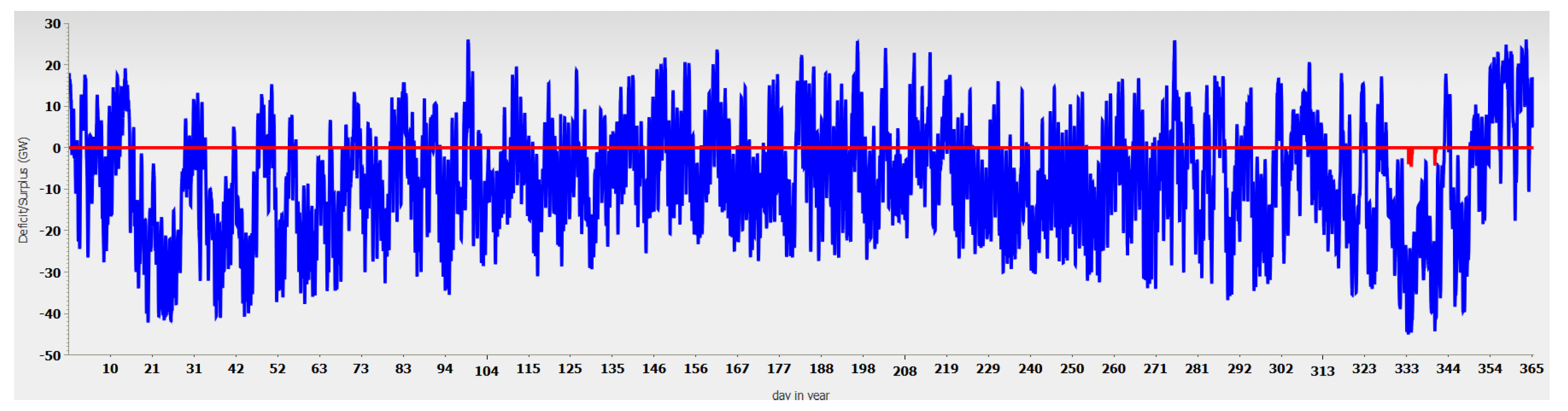
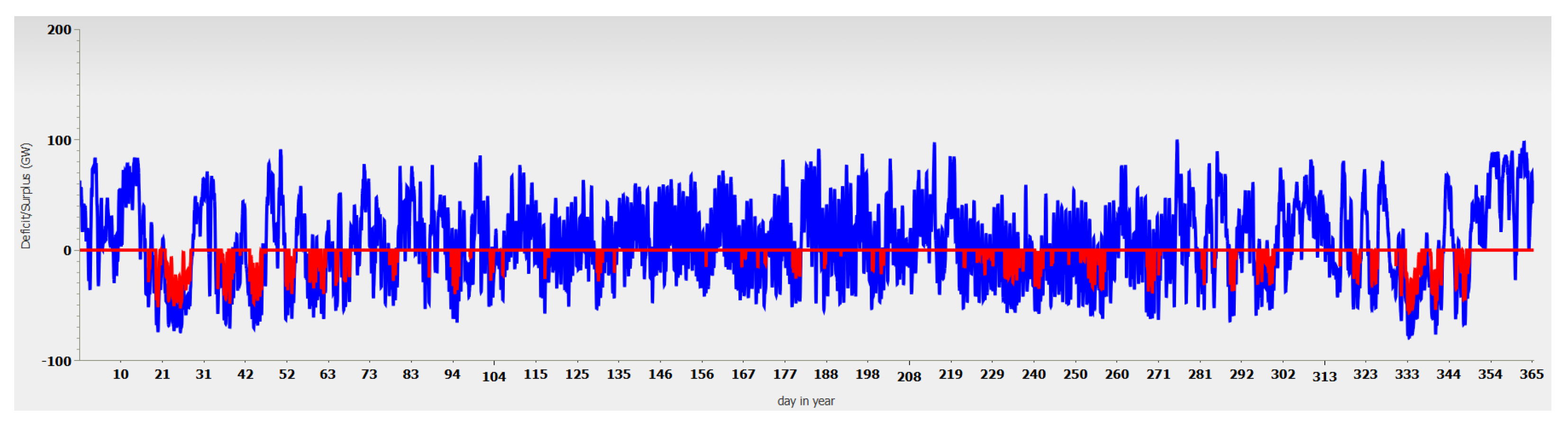
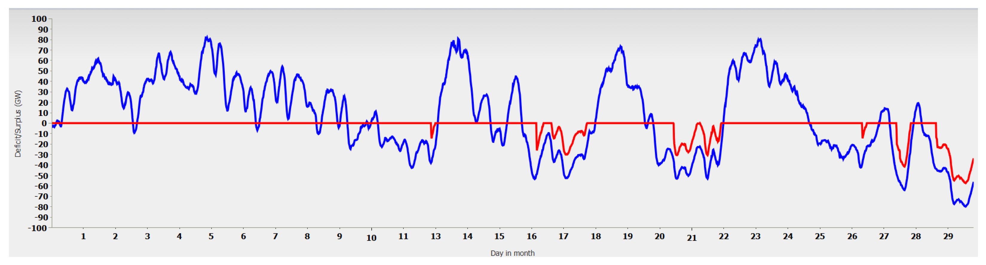
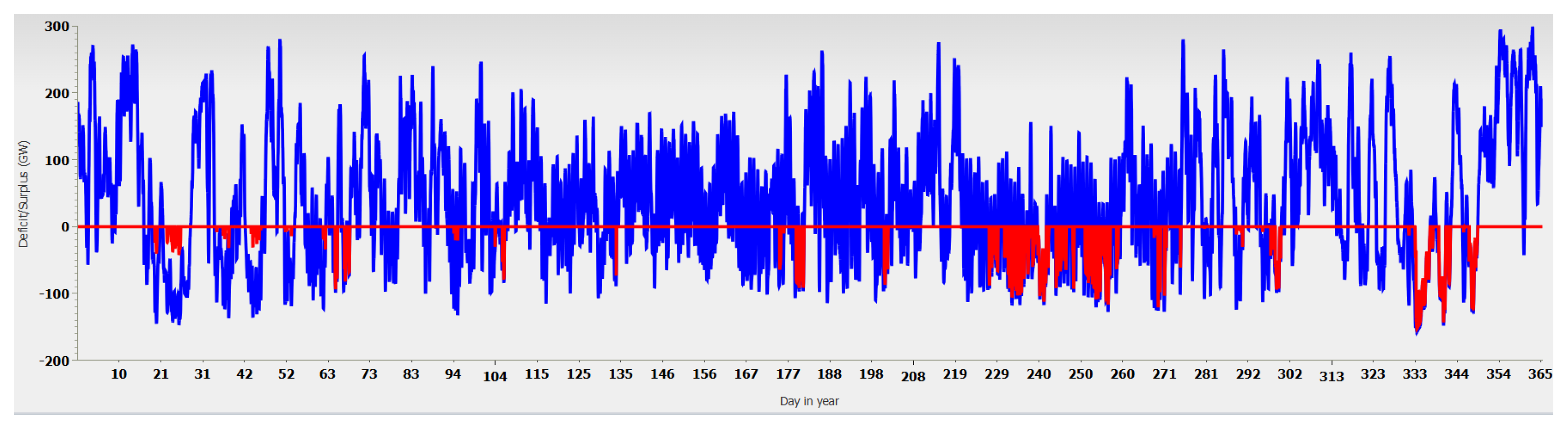
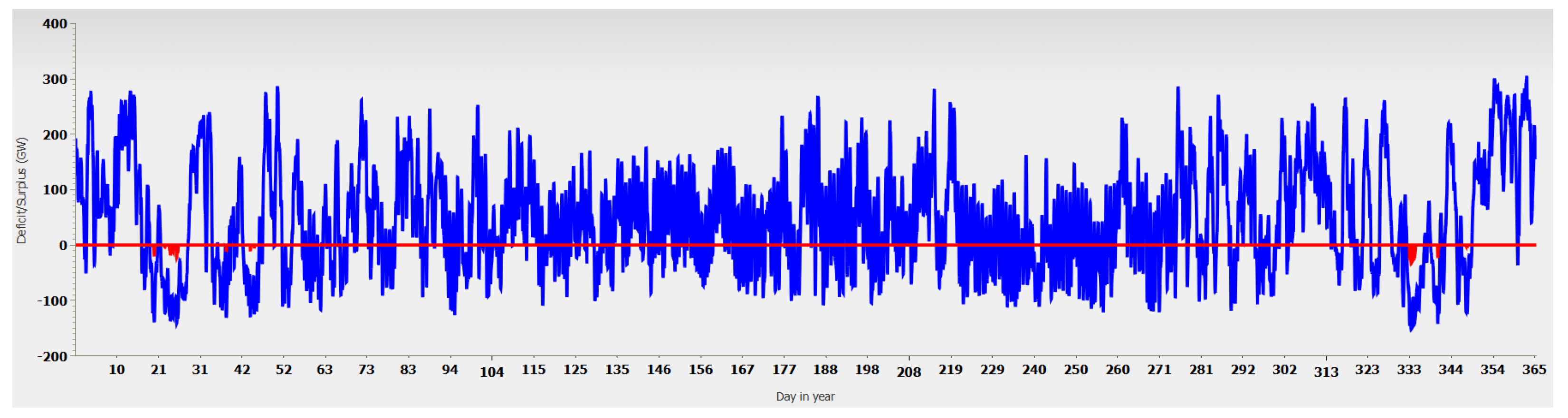
      Renewable Energy Volatility:
      *
      For each storage type (pumped, battery, gas), charts show surpluses (volatility > 0) and deficits (volatility < 0) in GW before (blue) and after (red) storage.
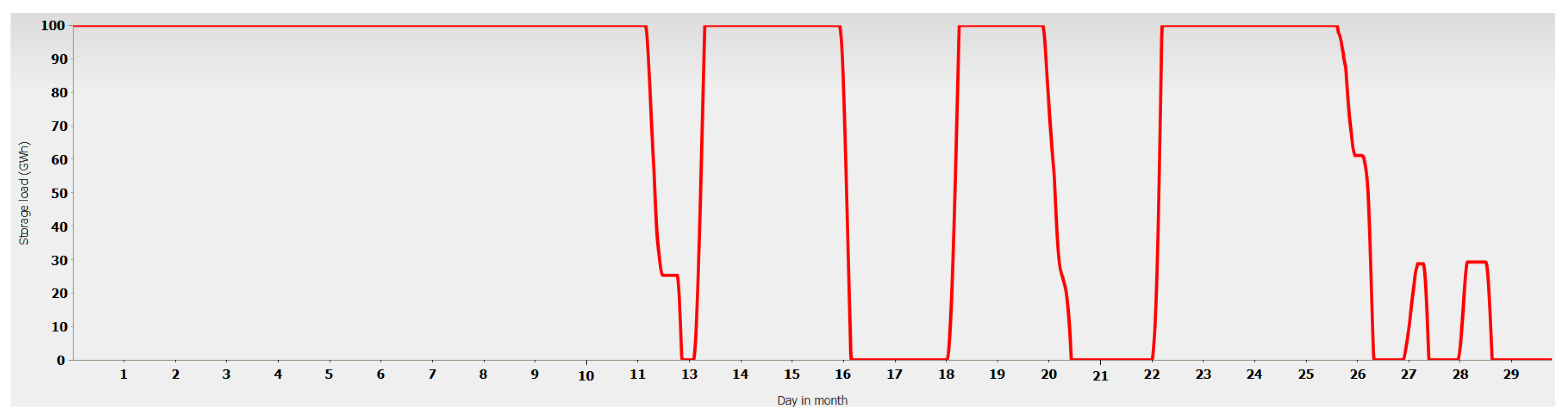
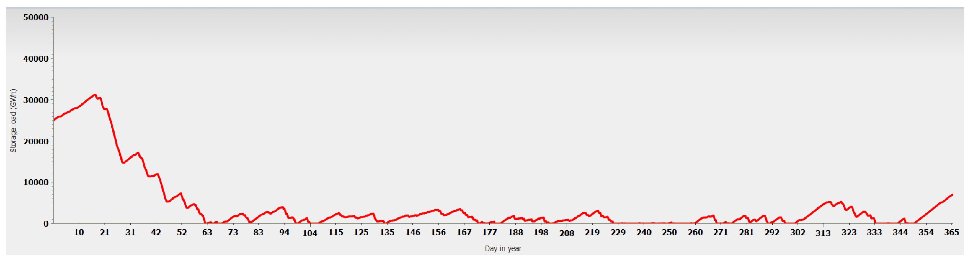
      Storage Charge Levels:
      *
      Charge levels (GWh) for pumped, battery, and gas storage over time.
      Energy Flow:
      *
      Energy flow into (red) and out of (blue) storage systems (GW) for each storage type.
      Residual Conventional Power Requirement:
      *
      Hours requiring conventional power, categorized by power capacity (GW).
    • Tables/Metrics:
      Energy Demand and Production:
      *
      Total demand (GWh).
      *
      Renewable production (total RE, wind + solar only) in GWh and % of demand.
      *
      Wind+solar directly usable, surplus (before/after storage), deficit (before/after storage), and full load hours.
      Baseload and Import/Export:
      *
      Reduced demand after fixed supply (GWh).
      *
      Contributions from hydro, biomass, nuclear, fossil backup, import, and export (GWh).
      Storage Metrics:
      *
      Energy flow into and out of storage systems (GWh).
      *
      Percentage of demand met by storage.
      Cost Metrics:
      *
      Specific costs for battery storage, gas storage (creation, storage, conversion), nuclear, and backup energy (EUR/MWh).
      *
      Shared costs for storage, PV, wind (onshore/offshore), biomass, nuclear, backup power, grid expansion, and subsidies (EUR/MWh).
      *
      Total shared cost of renewable energy (EUR/MWh).
  • User Interaction and Iteration
    • Users can adjust parameters (e.g., expansion factors, storage capacities, cost assumptions) and rerun the simulation to explore different scenarios.
    • The ability to drill down into monthly or daily data allows users to analyze specific periods simulation.
    • Scenario download/upload functionality enables users to save and share custom configurations.
  • Summary of Data Flow
    (a)
    Input Collection: Users select a scenario, dataset (Fraunhofer 2023/2024), time scope, and specify parameters for renewable expansion, consumption, storage, import/export, baseload power, and costs.
    (b)
    Simulation Execution: The tool processes inputs using a simplified model (copper plate assumption), calculating energy production, storage flows, and costs for the entire year. Surplus energy is curtailed, and storage balances volatility.
    (c)
    Output Generation: Results are displayed as charts (volatility, storage levels, energy flows) and tables (energy demand, production, storage, costs) for the selected time scope (year, month, or day).
    (d)
    Iteration: Users can modify parameters or scenarios, rerun the simulation, and download/upload configurations for further analysis.
This data flow enables users to explore optimistic energy transition scenarios, assess the role of storage and baseload power, and evaluate associated costs, with flexibility to customize and visualize results at different time scales.

References

  1. Enkard, S. Germany Records 457 Hours of Negative Electricity Prices in 2024. 2025. Available online: https://www.pv-magazine.com/2025/01/06/germany-records-457-hours-of-negative-electricity-prices-in-2024/ (accessed on 4 June 2025).
  2. Heimerl, S.; Kohler, B. Aktueller Stand der Pumpspeicher Kraftwerke in Deutschland. WasserWirtschaft 2017, 10, 77–79. [Google Scholar] [CrossRef]
  3. Weiß, M.; Wünsch, M.; Ziegenhagen, I. Klimaneutrales Deutschland 2045. 2021. Available online: https://www.agora-energiewende.de/fileadmin/Projekte/2023/2023-30_DE_KNDE_Update/A-EW_344_Klimaneutrales_Deutschland_WEB.pdf (accessed on 4 June 2025).
  4. Kuhlmann, A. Dena-Leitstudie Aufbruch Klimaneutralität. 2021. Available online: https://www.dena.de/infocenter/dena-leitstudie-aufbruch-klimaneutralitaet-1/ (accessed on 4 June 2025).
  5. Umweltbundesamt. Strommarkt und Klimaschutz: Transformation der Stromerzeugung bis 2050. 2021. Available online: https://www.umweltbundesamt.de/sites/default/files/medien/5750/publikationen/2021-02-17_cc_08-2021_transformation_stromerzeugung_2050_0.pdf (accessed on 4 June 2025).
  6. Wissenschaftlicher Dienst des Deutschen Bundestages. Zur Deckung des Zusätzlichen Strombedarfs Durch Erneuerbare Energien im Zuge der Energiewende. 2022. Available online: https://www.bundestag.de/resource/blob/890192/2396cb424eb80359f9d0494a563edabe/WD-5-026-22-pdf.pdf (accessed on 4 June 2025).
  7. Sinn, H.W. Buffering volatility: A study on the limits of Germany’s energy revolution. Eur. Econ. Rev. 2017, 99, 130–150. [Google Scholar] [CrossRef]
  8. Peters, B.; Watter, H.; Preusser, P.; Willner, T. Studie zur Klimaneutralität 2045: Offener Brief und Fragen zur Qualitätssicherung in öffentlichen Publikationen. 2021. Available online: https://www.energie-naturschutz.de/publikationen/studie-zur-klimaneutralitat-2045 (accessed on 4 June 2025).
  9. Peters, B.; Watter, H.; Preusser, P.; Willner, T. Replik auf Antwortschreiben Agora. 2021. Available online: https://www.energie-naturschutz.de/publikationen/replik-antwortschreiben-agora (accessed on 4 June 2025).
  10. Maier, K. Energiewende-Szenarien in Deutschland um 2045. 2025. Available online: https://magentacloud.de/s/x7LcTL7ckmcEByD (accessed on 4 June 2025).
  11. Maier, K. Dimensionierung Eines Ausschließlich auf Erneuerbaren Energien Basierenden Energiesystems in Deutschland. 2025. Available online: https://magentacloud.de/s/yt2eH6GacG5kBWm (accessed on 4 June 2025).
  12. Hansen, K.; Mathiesen, B.V.; Skov, I.R. Full energy system transition towards 100% renewable energy in Germany in 2050. Renew. Sustain. Energy Rev. 2019, 102, 1–13. [Google Scholar] [CrossRef]
  13. Gawel, E.; Lehmann, P.; Korte, K.; Strunz, S.; Bovet, J.; Köck, W.; Massier, P.; Löschel, A.; Schober, D.; Ohlhorst, D.; et al. The future of the energy transition in Germany. Energy Sustain. Soc. 2014, 4, 15. [Google Scholar] [CrossRef]
  14. Züttel, A.; Gallandat, N.; Dyson, P.; Schlapbach, L.; Gilgen, P.; Shin-ichi, O. Future Swiss Energy Economy: The Challenge of Storing Renewable Energy. Front. Energy Res. 2022, 9, 785908. [Google Scholar] [CrossRef]
  15. NZZ, Christoph Eisenring. Sechs Neue Kernkraftwerke? Studie der ETH Lausanne füHrt zu Einer Kontroverse. 2024. Available online: https://www.nzz.ch/wirtschaft/sechs-kernkraftwerke-studie-der-eth-lausanne-fuehrt-zu-einer-kontroverse-ld.1829743 (accessed on 4 June 2025).
  16. NREL. Power System Planning: Advancements in Capacity Expansion Modeling. 2021. Available online: https://www.nrel.gov/docs/fy21osti/80192.pdf (accessed on 4 June 2025).
  17. Nicoli, M.; Faria, V.A.D.; de Queiroz, A.R.; Savoldi, L. Modeling energy storage in long-term capacity expansion energy planning: An analysis of the Italian system. J. Energy Storage 2024, 101, 113814. [Google Scholar] [CrossRef]
  18. Löffler, K.; Hainsch, K.; Burandt, T.; Oei, P.Y.; Kemfert, C.; Von Hirschhausen, C. Designing a model for the global energy system—GENeSYS-MOD: An application of the open-source energy modeling system (OSeMOSYS). Energies 2017, 10, 1468. [Google Scholar] [CrossRef]
  19. Sarfarazi, S.; Sasanpour, S.; Cao, K. Improving energy system design with optimization models: Addressing the economic granularity gap in energy system modeling. Energy Rep. 2023, 9, 1859–1874. [Google Scholar] [CrossRef]
  20. Ruhnau, O.; Hirth, L.; Praktiknjo, A. Heating with wind: Economics of heat pumps and variable renewables. Energy Econ. 2020, 92, 104967. [Google Scholar] [CrossRef]
  21. Schöb, T.; Kullmann, F.; Linßen, J.; Stolten, D. The role of hydrogen for a greenhouse gas-neutral Germany by 2045. Int. J. Hydrogen Energy 2023, 48, 39124–39137. [Google Scholar] [CrossRef]
  22. Abuzayed, A.; Hartmann, N. MyPyPSA-Ger: Introducing CO2 taxes on a multi-regional myopic roadmap to a fully decarbonized German power system by 2050. Appl. Energy 2022, 310, 118576. [Google Scholar] [CrossRef]
  23. Brown, T.; Schlachtberger, D.; Kies, A.; Schramm, S.; Greiner, M. Synergies of sector coupling and transmission reinforcement in a cost-optimised, highly renewable European energy system. Energy 2018, 160, 720–739. [Google Scholar] [CrossRef]
  24. Schmidt, T.; Mangold, D.; Müller-Steinhagen, H. Seasonal Thermal Energy Storage in Germany. ISES Sol. World Congr. 2003. Available online: https://www.igte.uni-stuttgart.de/veroeffentlichungen/publikationen/publikationen_03-06.pdf (accessed on 4 June 2025).
  25. Popper, K.R. The Logic of Scientific Discovery; Hutchinson & Co.: London, UK, 1959. [Google Scholar]
  26. Peters, B.R. Schluss mit der Energiewende! Peters Coll. Beratungs-und-Beteiligungs-GmbH: Berlin, Germany, 2025. [Google Scholar]
  27. Peters, B. Der Erhalt von sechs Kernkraftwerken könnte den Großhandelspreis für Strom um die Hälfte absenken. ATW 2022, 68, 2–5. [Google Scholar]
  28. Ahlborn, D.; Ahlborn, F. Storage size estimation for volatile renewable power generation: An application of the Fokker–Planck equation. Eur. Phys. J. Plus 2023, 138, 401. [Google Scholar] [CrossRef]
  29. Dengler, J. Online Simulator of the German Energy Transition. 2025. Available online: https://www.cortima.com/energiewende/energytransition.html (accessed on 4 June 2025).
  30. Fraunhofer Institute for Solar Energy Systems ISE. Energy Charts. 2025. Available online: https://www.energy-charts.info/?l=en&c=DE (accessed on 4 June 2025).
  31. Battery University. BU-402: What Is C-Rate? 2021. Available online: https://batteryuniversity.com/article/bu-402-what-is-c-rate (accessed on 4 June 2025).
  32. Energy Information Administration. Utility-Scale Batteries and Pumped Storage Return About 80% of the Electricity They Store. 2021. Available online: https://www.eia.gov/todayinenergy/detail.php?id=46756 (accessed on 4 June 2025).
  33. BDEW Bundesverband der Energie- und Wasserwirtschaft e.V. Zahl der Woche/Bis zu 254,8 Milliarden Kilowattstunden Erdgas. 2023. Available online: https://www.bdew.de/presse/presseinformationen/zahl-der-woche-bis-zu-2548-milliarden-kilowattstunden-erdgas/ (accessed on 4 June 2025).
  34. Initiative Energie Speichern (INES). Saubere Energien in Gas und Wasserstoffspeichern. 2025. Available online: https://energien-speichern.de/positionen/umweltvertraeglichkeit/saubere-energien-in-gas-und-wasserstoffspeichern/ (accessed on 4 June 2025).
  35. Bossel, U. Wasserstoff löst Keine Energieprobleme. 2021. Available online: https://leibniz-institut.de/archiv/bossel_16_12_10.pdf (accessed on 4 June 2025).
  36. Bossel, U.; Eliasson, B.; Taylor, G. The Future of the Hydrogen Economy: Bright or Bleak? Cogener. Distrib. Gener. J. 2003, 18, 29–70. [Google Scholar] [CrossRef]
  37. Peters, B. Wasserstoff, Energieträger der Zukunft. Oder? 2019. Available online: https://deutscherarbeitgeberverband.de/Artikel.html?PR_ID=830 (accessed on 4 June 2025).
  38. Peters, B. Wasserstoffwirtschaft: Günstige Quellen müssen Her! 2020. Available online: https://deutscherarbeitgeberverband.de/Artikel.html?PR_ID=853 (accessed on 4 June 2025).
  39. Kopernikus-Projekte, Bundesministerium für Bildung und Forschung. Anforderungsprofile (für den Einsatz von Lastflexibilisierung). 2025. Available online: https://synergie-projekt.de/ergebnis/anforderungsprofile (accessed on 4 June 2025).
  40. Stede, J. Demand Response in Germany: Technical Potential, Benefits and Regulatory Challenges. 2016. Available online: https://www.diw.de/de/diw_01.c.532829.de/publikationen/roundup/2016_0096/demand_response_in_germany__technical_potential__benefits_and_regulatory_challenges.html (accessed on 4 June 2025).
  41. Deutsche Energie-Agentur. Flexibility Technologies and Measures in the German Power System. 2021. Available online: https://www.dena.de/fileadmin/dena/Dokumente/Projektportrait/Projektarchiv/Entrans/Flexibility_Technologies_and_Measures_in_the_German_Power_System_EN.pdf (accessed on 4 June 2025).
  42. Bender, J.; Fait, L.; Wetzel, H. Acceptance of demand-side flexibility in the residential heating sector—Evidence from a stated choice experiment in Germany. Energy Policy 2024, 191, 114145. [Google Scholar] [CrossRef]
  43. Katanich, D. Norway Aims to Cut Energy Links with Europe Due to Soaring Prices. 2024. Available online: https://www.euronews.com/business/2024/12/13/norway-aims-to-cut-energy-links-with-europe-due-to-soaring-prices (accessed on 4 June 2025).
  44. Czisch, G. Szenarien zur Zukünftigen Stromversorgung, Kostenoptimierte Variationen zur Versorgung Europas und Seiner Nachbarn mit Strom aus Erneuerbaren Energien. 2006. Available online: https://kobra.uni-kassel.de/items/cade2566-0243-481e-9e49-eb3ef90b27c9 (accessed on 4 June 2025).
  45. Loulou, R.; Goldstein, G.; Kanudia, A.; Lettila, A.; Remme, U. Documentation for the TIMES Model: Part I—Concepts and Theory. In Energy Technology Systems Analysis Programme (ETSAP); IEA-ETSAP: Paris, France, 2016. [Google Scholar]
  46. Hess, D.; Wetzel, M.; Cao, K.K. Representing node-internal transmission and distribution grids in energy system models. Renew. Energy 2018, 119, 874–890. [Google Scholar] [CrossRef]
  47. MAN Energy Solutions. Produce Greener Energy with Hybrid Power Plants. 2025. Available online: https://web.archive.org/web/20250505022054/https://www.man-es.com/energy-storage/solutions/hybrid-power (accessed on 4 June 2025).
  48. ENTSO-E. Frequency Stability Analysis in Long-Term Scenarios: Relevant Solutions and Mitigation Measures; Technical Report; European Network of Transmission System Operators for Electricity: Brussels, Belgium, 2023. [Google Scholar]
  49. Milano, F.; Dörfler, F.; Hug, G.; Hill, D.J.; Verbič, G. Foundations and Challenges of Low-Inertia Systems. In Proceedings of the 2018 Power Systems Computation Conference (PSCC), Dublin, Ireland, 11–15 June 2018; pp. 1–25. [Google Scholar] [CrossRef]
  50. Bundesnetzagentur. Bundesnetzagentur Publishes 2024 Electricity Market Data. 2025. Available online: https://www.bundesnetzagentur.de/SharedDocs/Pressemitteilungen/EN/2025/20250103_SMARD.html (accessed on 4 June 2025).
  51. Bundesverband Windenergie. Windenergie in Deutschland. 2025. Available online: https://www.wind-energie.de/themen/zahlen-und-fakten/deutschland/ (accessed on 4 June 2025).
  52. Maas, O.; Raasch, S. Wake properties and power output of very large wind farms for different meteorological conditions and turbine spacings: A large-eddy simulation case study for the German Bight. Wind Energy Sci. 2022, 7, 715–739. [Google Scholar] [CrossRef]
  53. Hilly, M.; Rettberg, N.J.; Ollington, R.; Nelson, M. Restarting Germany’s Reactors: Feasibility and Schedule; Technical Report; Radiant Energy Group: Chicago, IL, USA, 2024. [Google Scholar]
Figure 1. Energy mix and demand time series of week 13, 2025 from Fraunhofer ISE Energy Charts.
Sustainability 17 05295 g001
Figure 2. Volatility of existing renewable energy sources in 2023. Blue graph before process, red graph after process.
Sustainability 17 05295 g002
Figure 3. Volatility of the planned renewable energy in 2030. Blue graph before process, red graph after process.
Sustainability 17 05295 g003
Figure 4. Volatility of the planned renewable energy in November 2030. Blue graph before process, red graph after process.
Sustainability 17 05295 g004
Figure 5. Battery load state of the November 2030 scenario.
Sustainability 17 05295 g005
Figure 6. Required hours of additional power in 2030.
Sustainability 17 05295 g006
Figure 7. Volatility of the planned renewable energy in November 2030. Backup power changed to 50 GW. Blue graph before process, red graph after process.
Sustainability 17 05295 g007
Figure 8. Volatility of the planned renewable energy in 2045. Blue graph before process, red graph after process.
Sustainability 17 05295 g008
Figure 9. Gas storage load state in the 2045 scenario.
Sustainability 17 05295 g009
Figure 10. Volatility of the adapted renewable energy scenario for 2045. Blue graph before process, red graph after process.
Sustainability 17 05295 g010
Figure 11. Gas storage load state of the adapted renewable.
Sustainability 17 05295 g011
Table 1. Potential of demand-side management in Germany.
SectorTechn. PotentialActivation DurationKey Technologies
Heavy Industry5–15 GW1–8 hAluminum smelters,
cement kilns
SMEs2–7 GW30 min–2 hRefrigeration,
ventilation
Households3–30 GW15 min–4 hHeat pumps, EVs,
smart appliances
Table 2. Planned expansion of Wind and PV according to Agora.
DescriptionUnit202320302045
Installed power PVGW82215469
Installed power wind onshoreGW6198180
Installed power wind offshoreGW82673
Expected Energy PV + wind + hydroTWh2195071087
Expected Energy biomass and hydrogenTWh505092
Expected Energy others (garbage, nuclear, geothermal)TWh2903
Expected Energy coal and natural gasTWh1921320
Expected Energy battery storageTWh02059
Net demandTWh4897091241
Disclaimer/Publisher’s Note: The statements, opinions and data contained in all publications are solely those of the individual author(s) and contributor(s) and not of MDPI and/or the editor(s). MDPI and/or the editor(s) disclaim responsibility for any injury to people or property resulting from any ideas, methods, instructions or products referred to in the content.

