
A New Hybrid Framework for the MPPT of Solar PV Systems Under Partial Shaded Scenarios

 , , and
Abstract
1. Introduction
- A new hybrid framework is proposed that leverages the strengths of both the ANN and FOPID controller for solar MPPT applications. A modified Shuffled Frog Leaping Algorithm (MSFLA) is employed to train the ANN model for various values of temperature (T) and irradiance (G). Additionally, the Sanitized Teacher–Learning-Based Optimization (s-TLBO) algorithm is introduced to tune the FOPID controller, aiming to efficiently regulate the duty cycle.
- Furthermore, tailored parameter modifications, such as variable step-size scaling, are introduced in the MSFLA. This enhancement helps avoid local minima during ANN training and accelerates convergence, particularly under nonlinear conditions like partial shading.
- The proposed framework accurately predicts the reference voltage under different environmental conditions and consistently delivers superior output across various scenarios and for different types of solar panels (monocrystalline and polycrystalline), demonstrating its robustness.
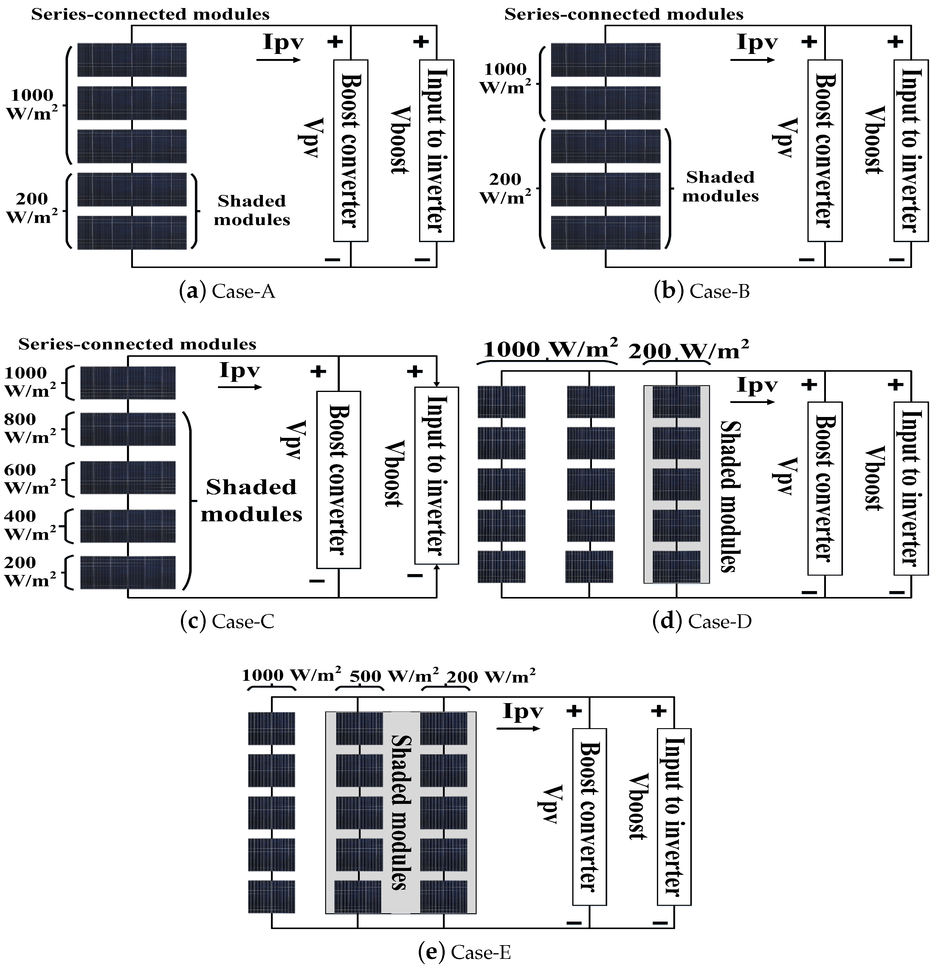
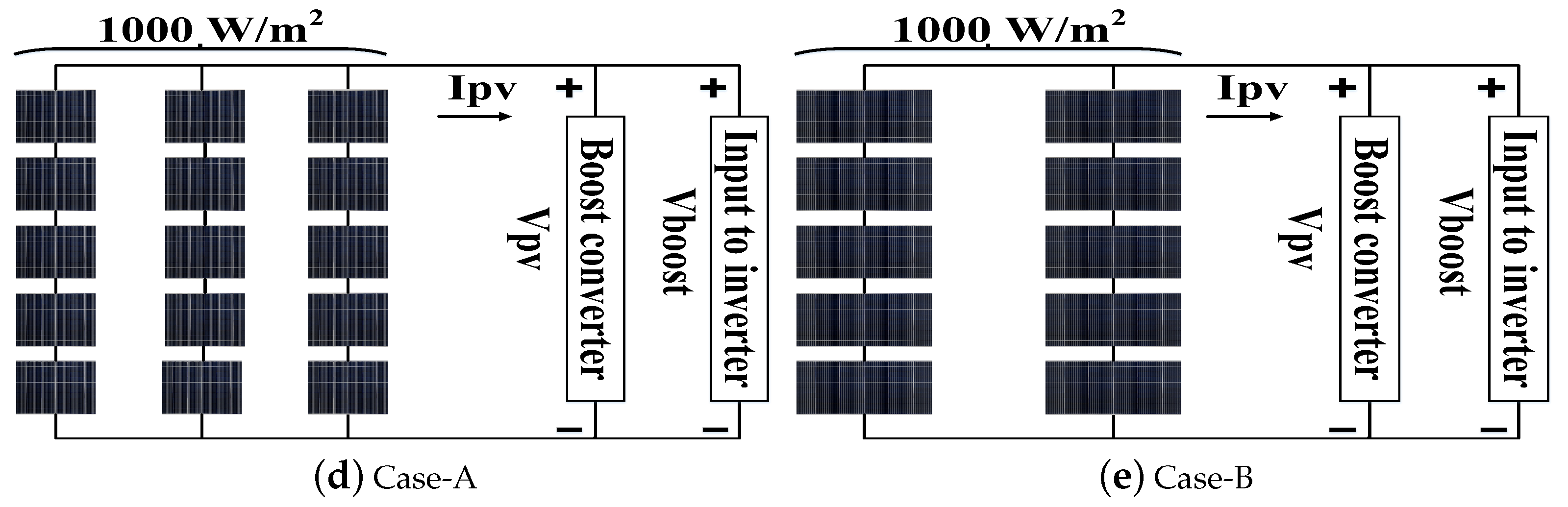
- It is finally validated by applying the proposed framework to different solar array configurations, namely, 5 × 1, 5 × 2, and 5 × 3 panel arrangements, under various partial shading conditions. The corresponding P–V and I–V characteristics curves are plotted, clearly illustrating the maximum power obtained for each case considered.
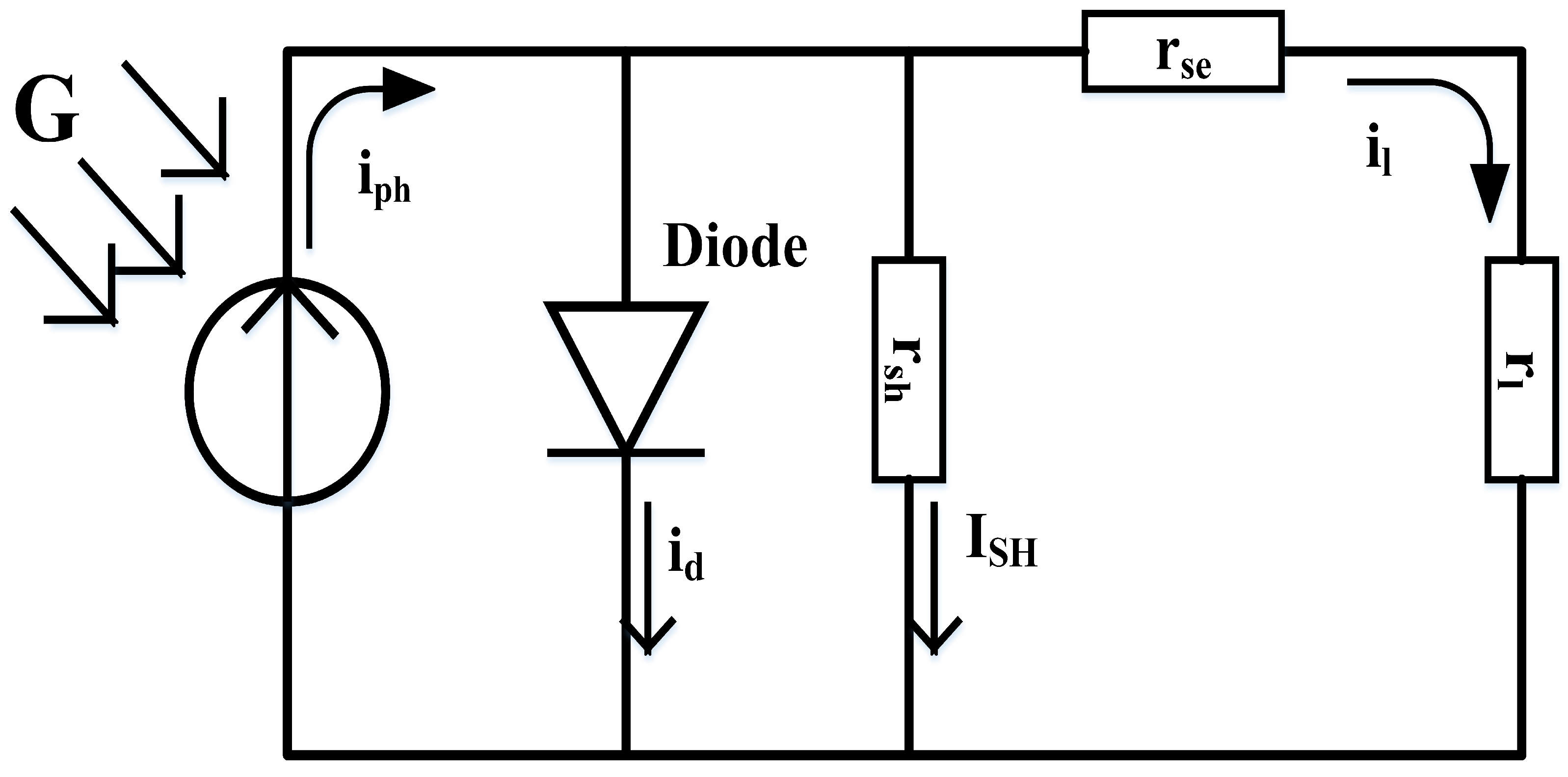
2. Solar PV Model
- = load voltage;
- = load current;
- = photon current;
- = saturation current;
- = series resistance;
- = shunt resistance;
- = thermal voltage ().
- = photo generated current (A);
- = reference temperature;
- = reference irradiance;
- T = absolute temperature;
- = SC current temperature coefficient (A/K) under standard test conditions;
- G = irradiance (W/).
3. Preliminaries
3.1. Artificial Neural Network (ANN)
- = input;
- = weights;
- = bias.
- N = no. of input data;
- M = no. of output data;
- = calculated output;
- = desired output.
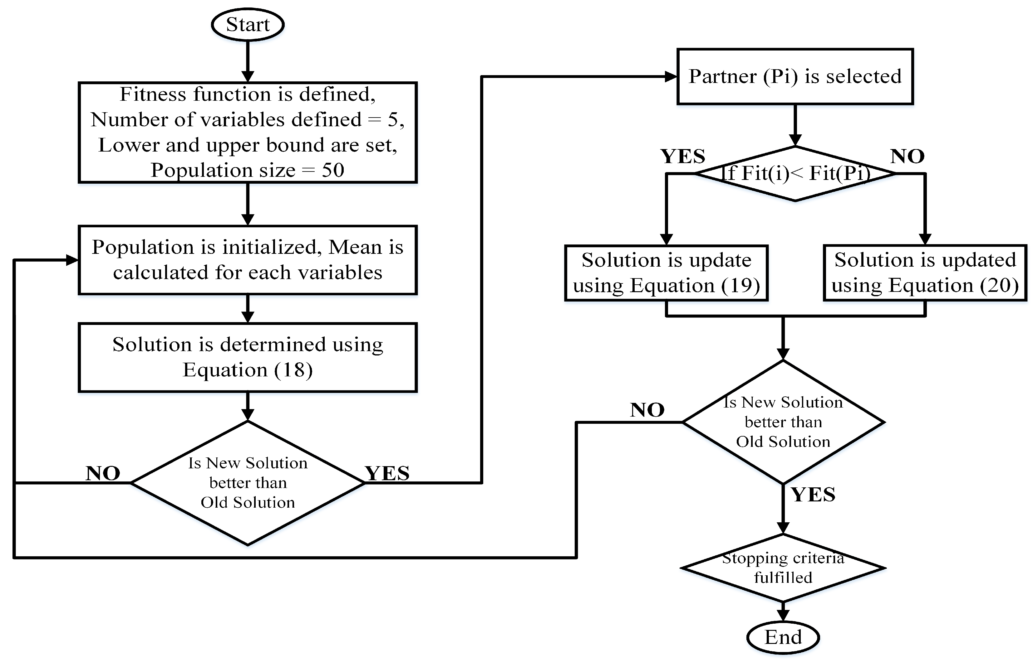
3.2. Sanitized Teacher–Learning-Based Optimization
3.2.1. Teacher Phase
3.2.2. Learner Phase
3.3. FOPID Controller
3.4. DC–DC Boost Converter
- Inductance (L) = 10 mH;
- Capacitance (C) = 500 μF;
- Resistance (R) = 25 ohms.
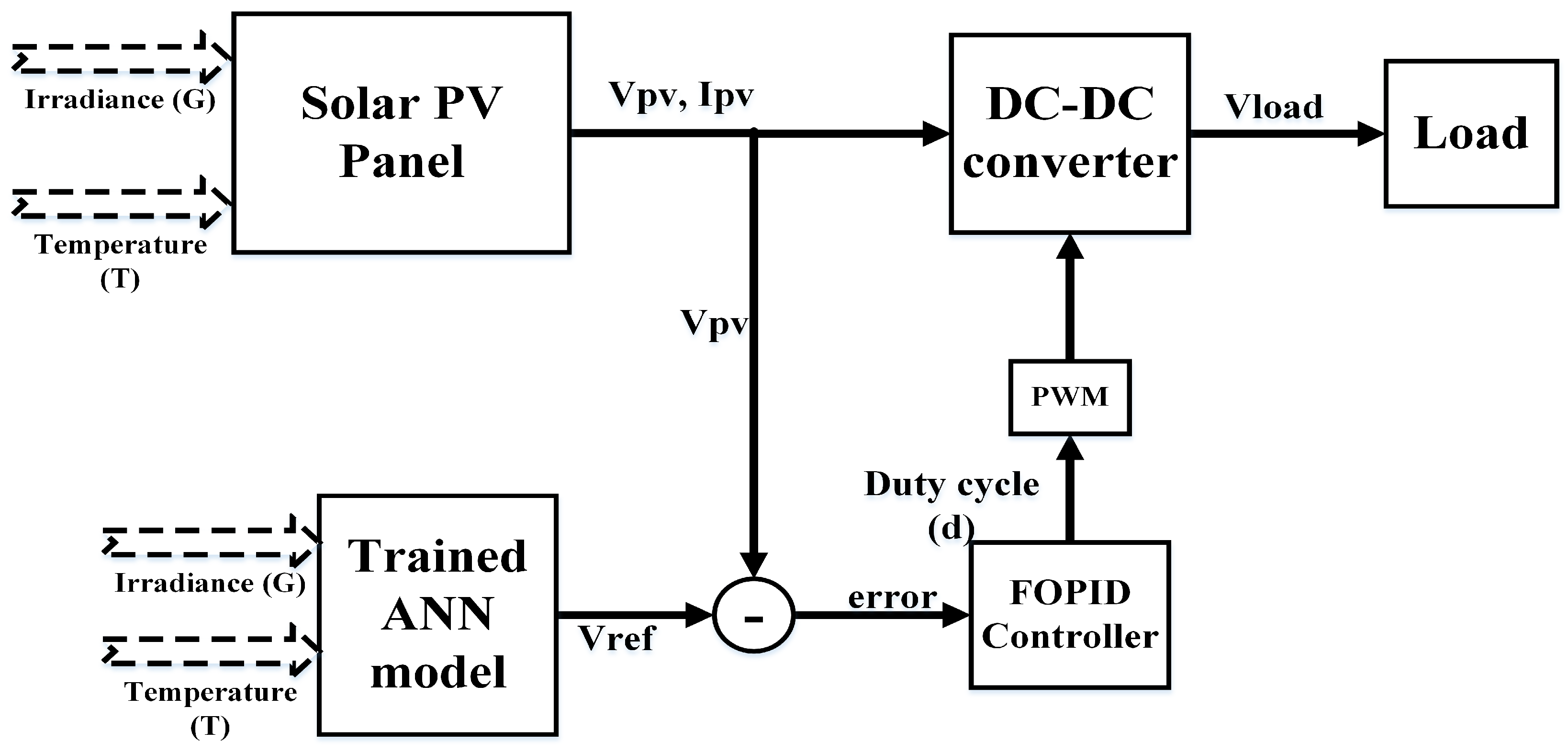
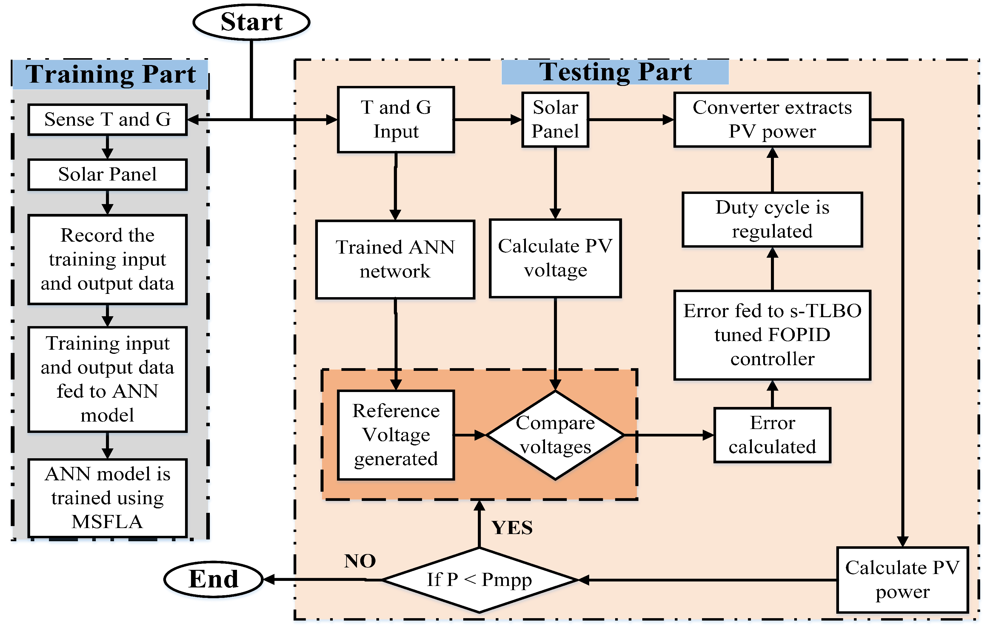
4. Proposed Hybrid-Framework
- An artificial neural network (ANN) trained using a Modified Shuffled Frog Leaping Algorithm (MSFLA), and
- A fractional-order PID (FOPID) controller dynamically tuned using a sanitized Teacher–Learning-Based Optimization (s-TLBO) algorithm.
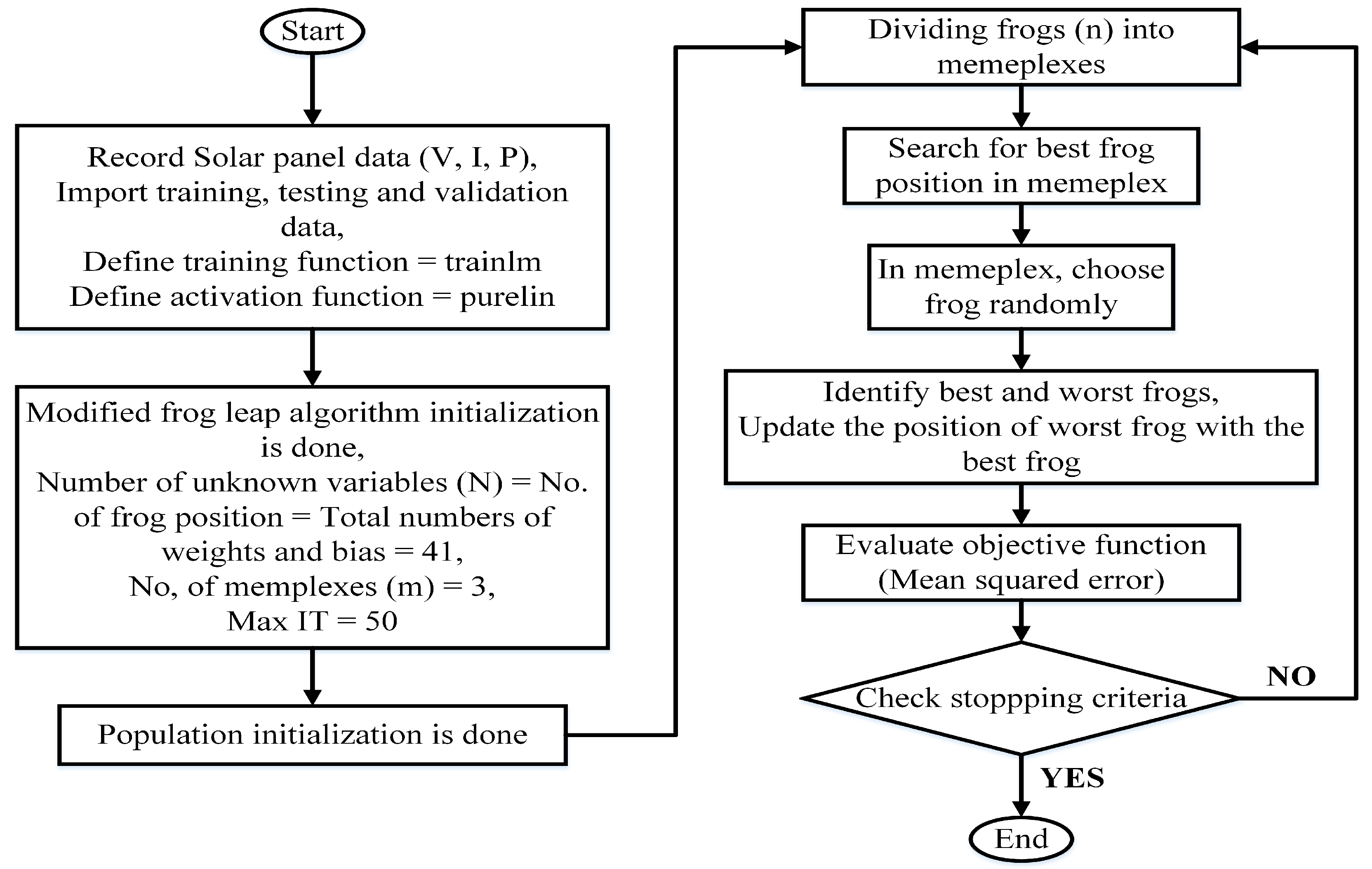
4.1. MSFLA-Based Trained ANN
- Number of weights = 30;
- Number of bias = 11;
- Learning rate () = 0.05;
- ANN training function = ‘trainlm’;
- ANN activation function = ‘Levenberg–Marquardt’;
- Number of unknown variables = 41;
- Number of memeplexes = 3;
- Number of frogs in each memeplex = 3;
- Maximum iteration = 50;
- Constant values, = = 1.5, w = 1.2.
- Variable step size scaling (s) for each frog is carried out and it is mathematically expressed in Equation (9),
4.2. FOPID Tuned Using s-TLBO
- = 100;
- Unknown variables (D) = 5;
- Upper limit (UL) = [4 4 4 1 1];
- Lower limit (LL) = [0 0 0 0 0];
- Max Iteration (i) = 100.
5. Computational Result Studies
- Relative error (RE) is a measure used to quantify the accuracy by comparing the calculated value with the true value. In the proposed work, relative error is measured by comparing the calculated power with the actual peak power.where is the peak power calculated and is the actual peak power of the panel.
- MPP efficiency is the measure of the precision obtained in measuring the actual peak power for the particular operating condition. It is expressed as
- Tracking speed is the measure of the speed by which the curve reaches its global peak and it is measured in seconds.
- Root mean squared error (RMSE) measures the average magnitude of the errors between the calculated values and the actual values. The smaller the RMSE, the better the model is at calculating the values.
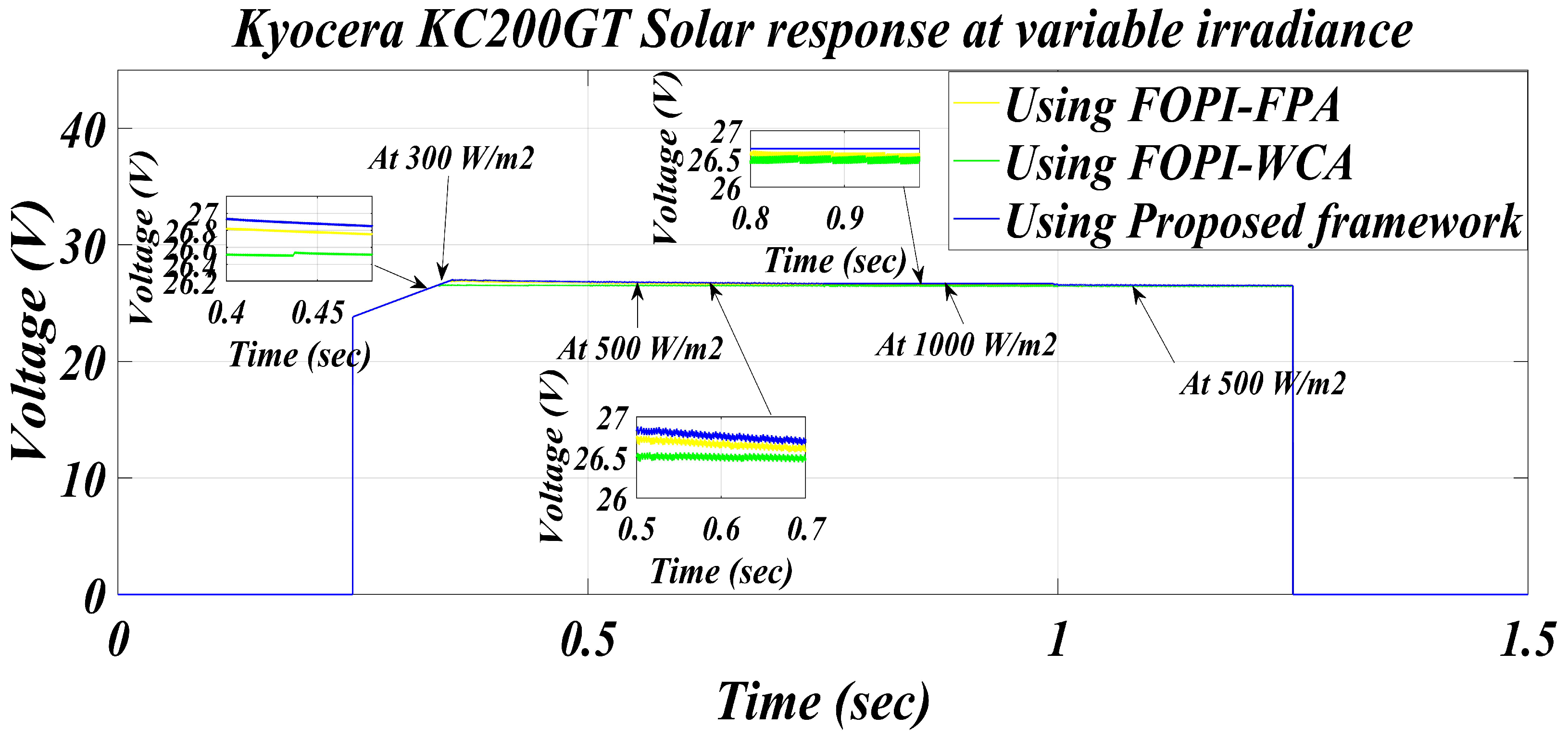
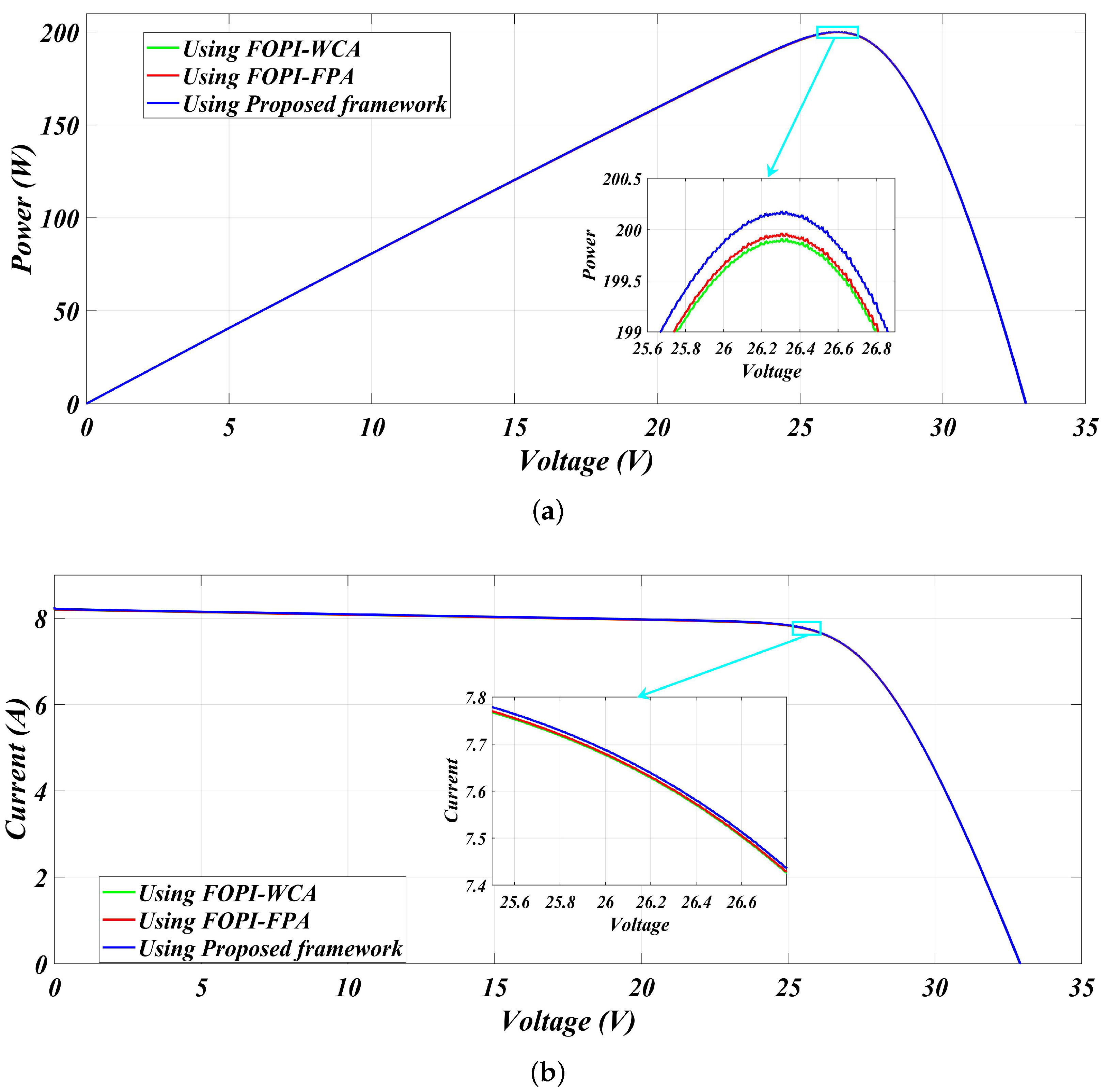
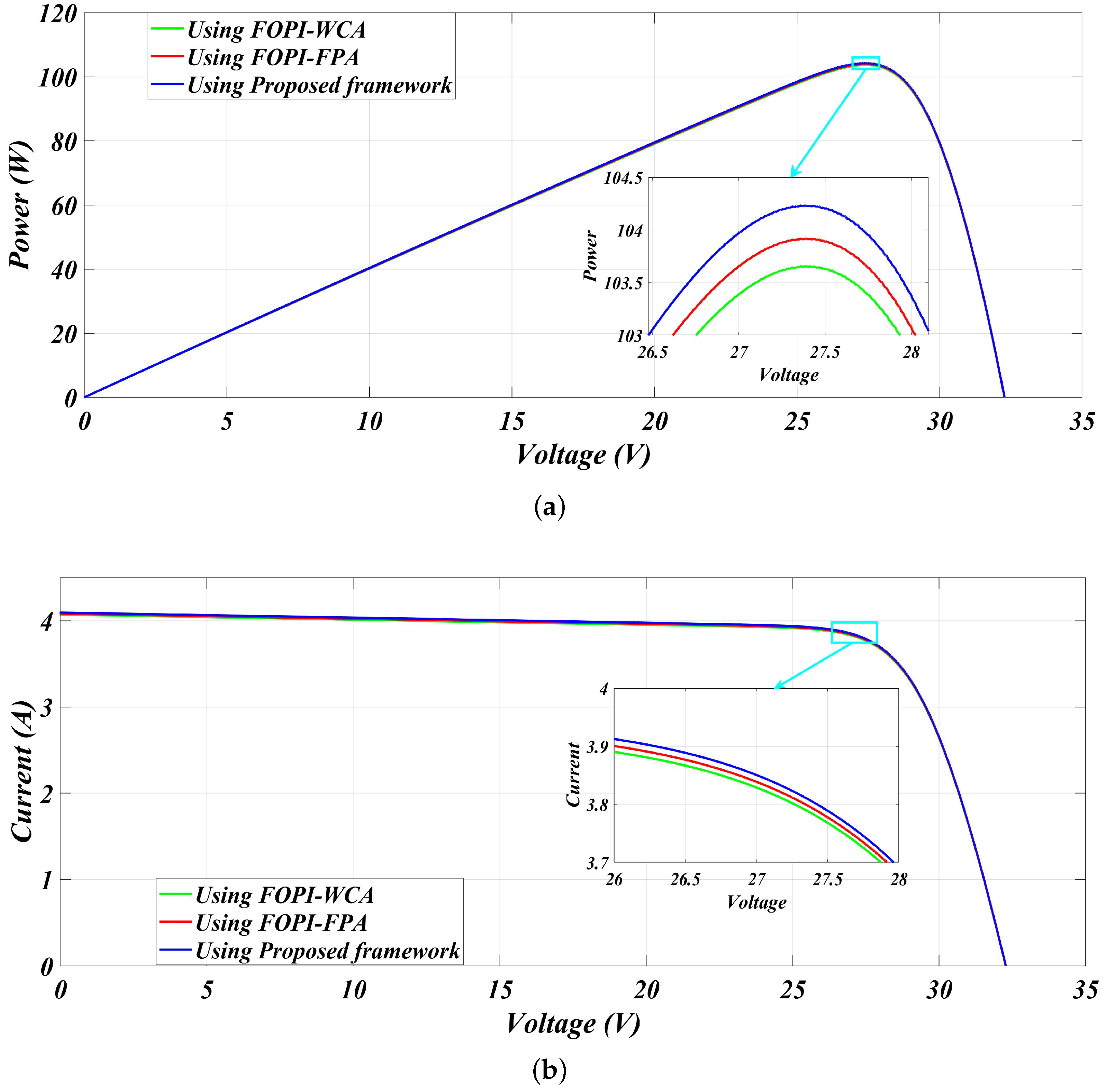
5.1. Solar Panel-1
5.1.1. Scenario-1
5.1.2. Scenario-2
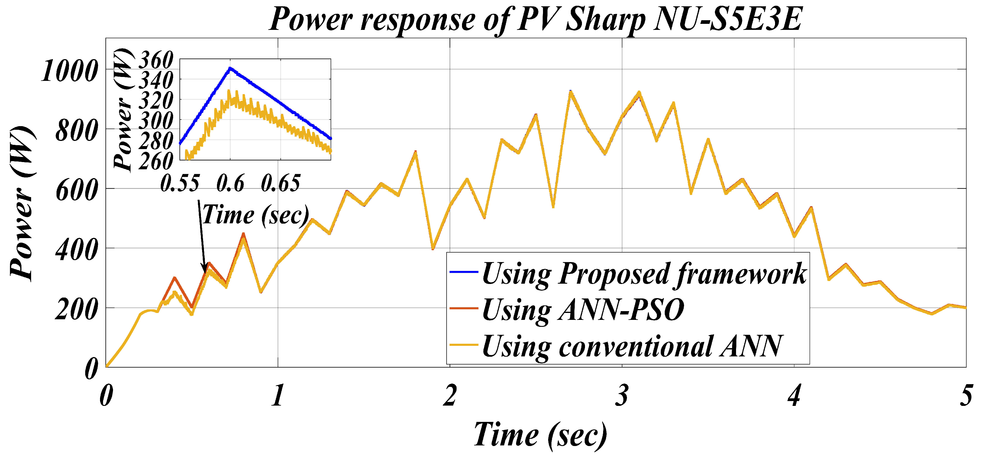
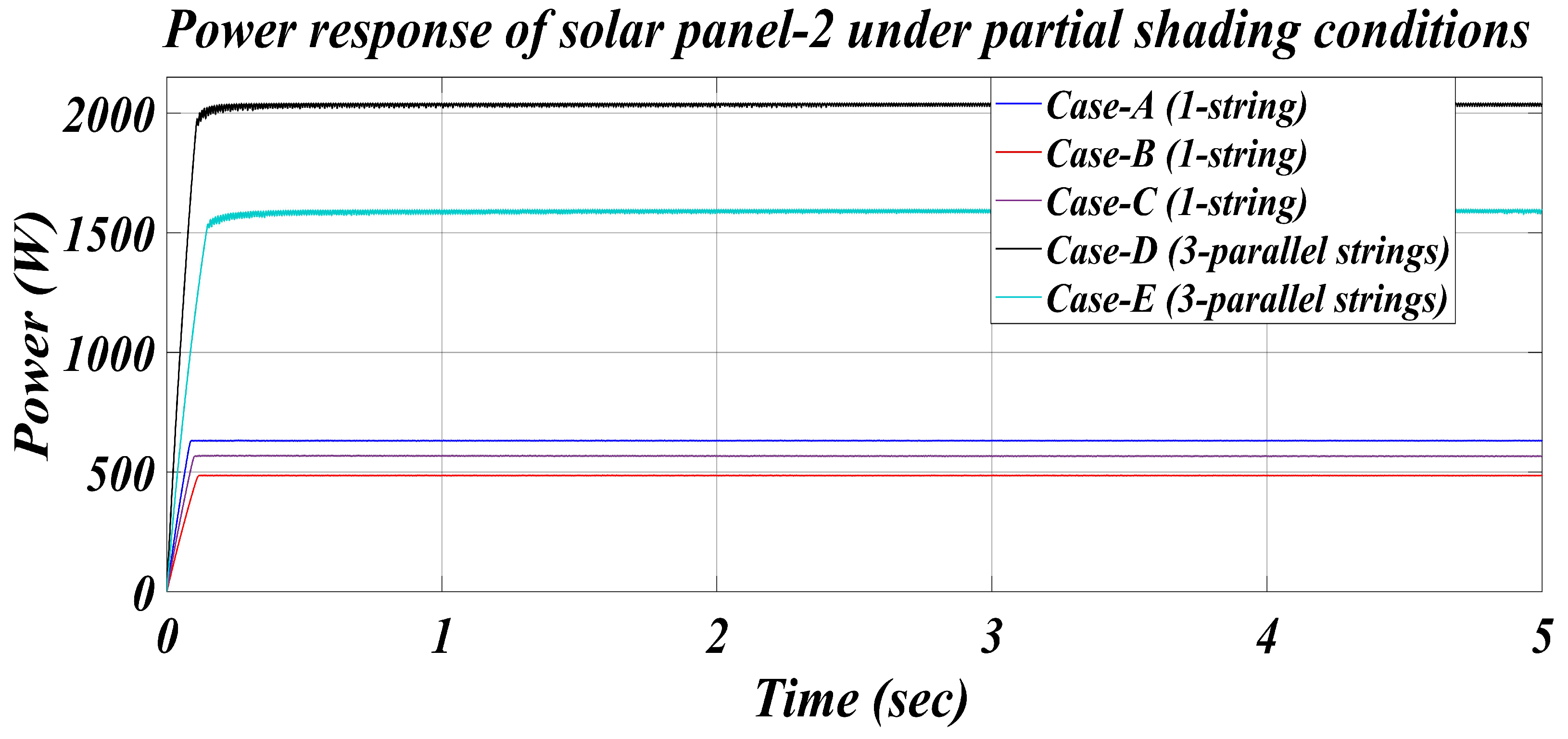
5.2. Solar Panel-2
5.2.1. Scenario-1
5.2.2. Scenario-2
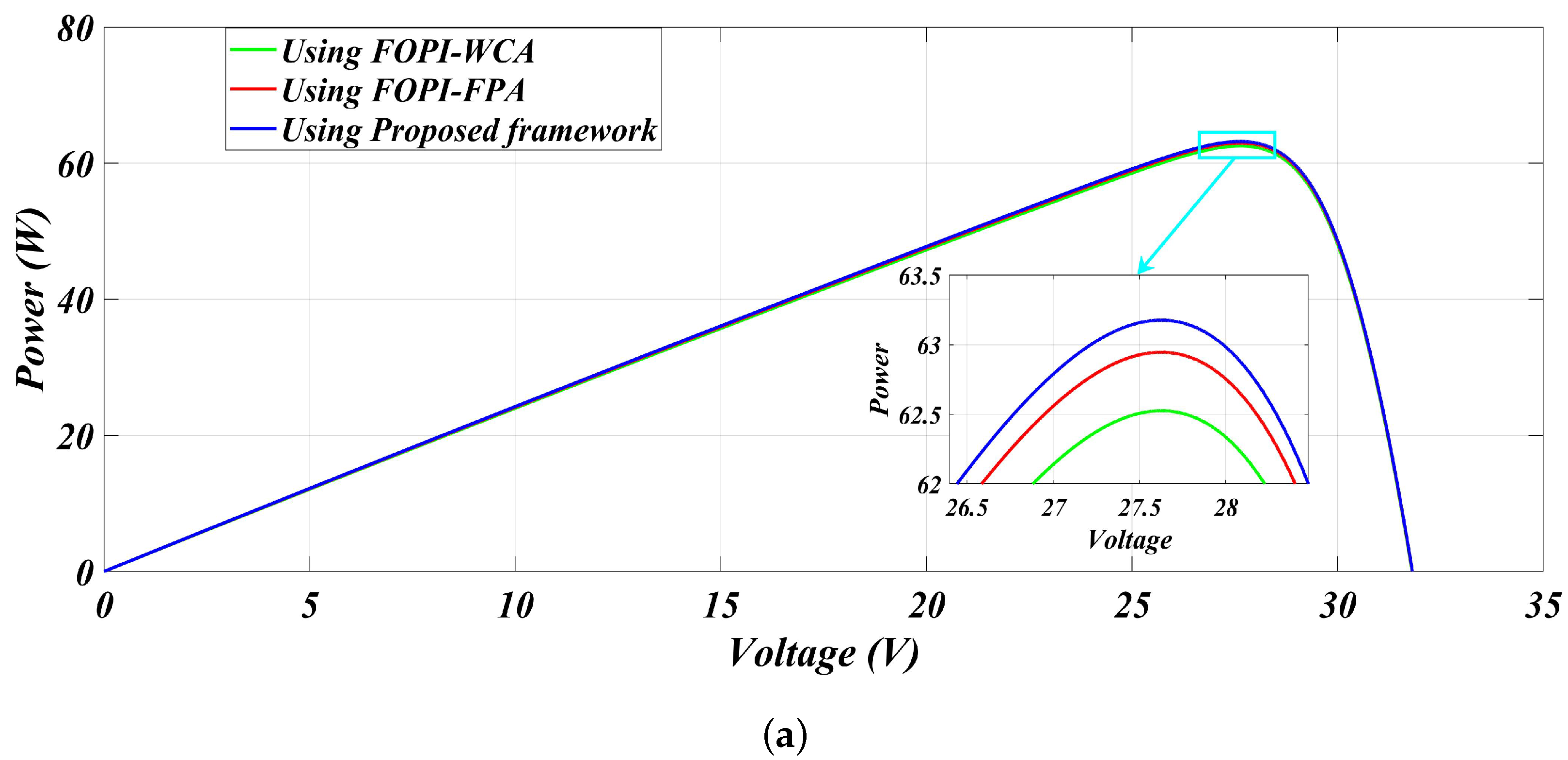
5.2.3. Scenario-3
- +1.04% over WCA at 300 W/m2.
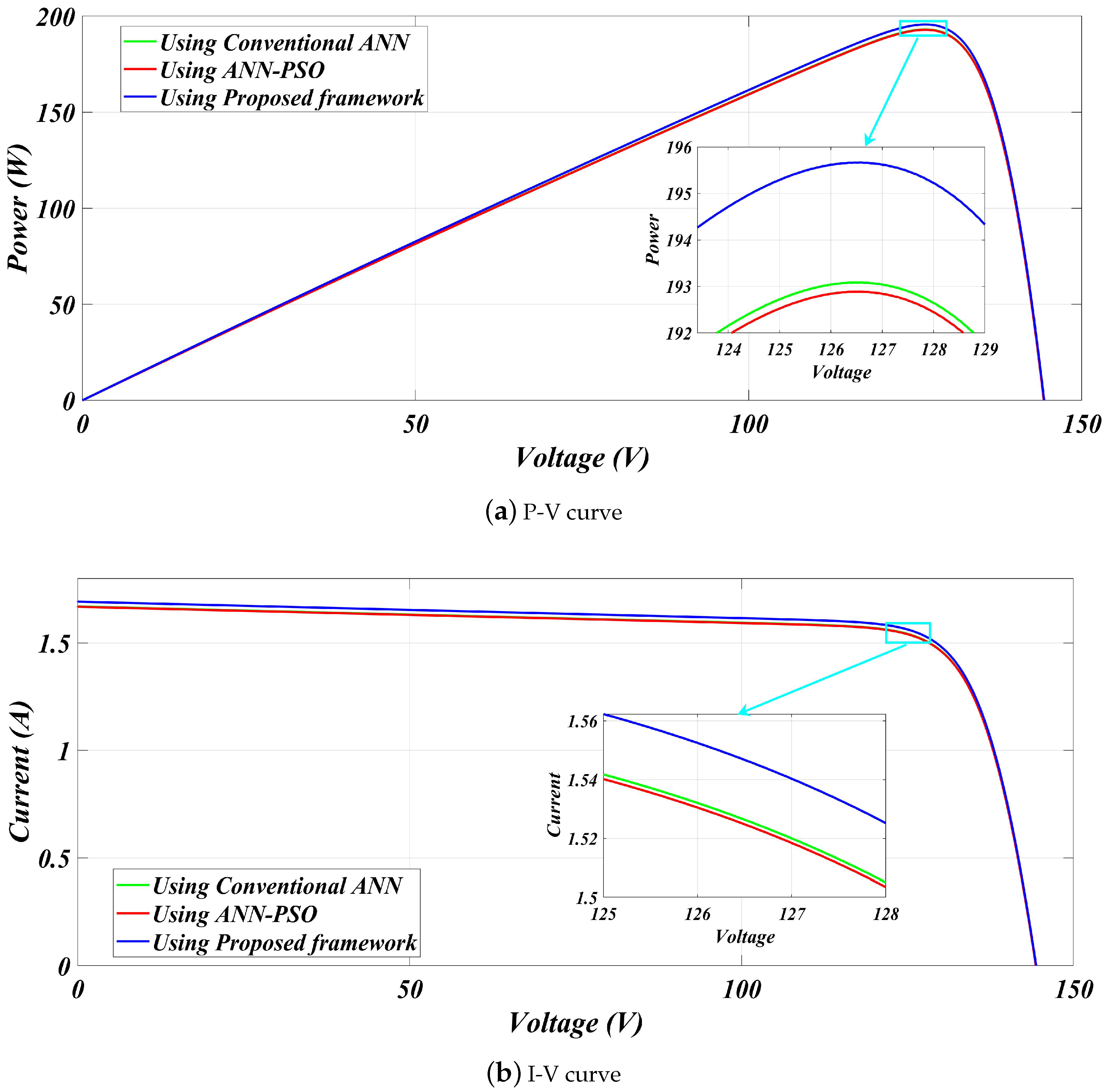
- +1.41% over ANN-PSO and +1.34% over conventional ANN at 200 W/m2.
6. Conclusions
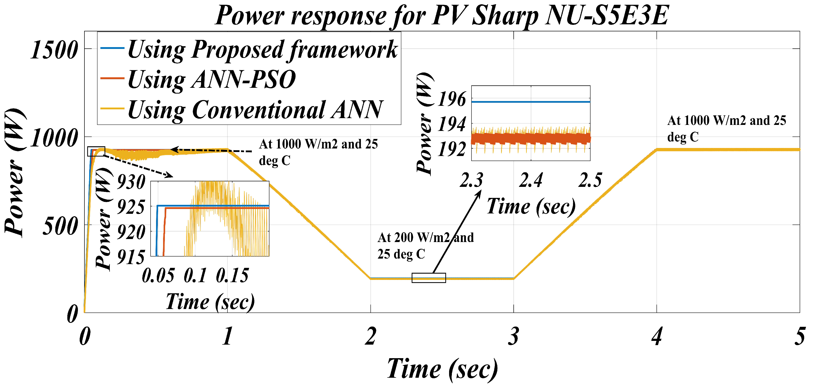
- To further assess its robustness, the framework was applied to an array configuration of solar panel-2. This evaluation included testing under various environmental conditions, such as cloudy weather and different partial shading scenarios. The framework was also tested on array configurations of 5 × 1, 5 × 2, and 5 × 3, yielding improved performance relative to prior studies, as shown in Table 5, Table 6, Table 7, Table 8 and Table 9. Notably, the proposed approach achieved fast and stable MPP tracking within 0.049 s, with minimal oscillations.
- The effectiveness of the proposed framework was further validated through rigorous simulations conducted using MATLAB software.
Author Contributions
Funding
Institutional Review Board Statement
Informed Consent Statement
Data Availability Statement
Conflicts of Interest
References
- Invest India. Renewable Energy. 2024. Available online: https://www.investindia.gov.in/sector/renewable-energy (accessed on 1 July 2022).
- Fazal, M.R.; Abbas, Z.; Kamran, M.; Ul Haq, I.; Ayyaz, M.N.; Mudassar, M. Modified Perturb and Observe MPPT algorithm for partial shading conditions. Int. J. Renew. Energy Resour. 2019, 9, 721–731. [Google Scholar]
- Pillai, D.S.; Rajasekar, N.; Ram, J.P.; Chinnaiyan, V.K. Design and testing of two phase array reconfiguration procedure for maximizing power in solar PV systems under partial shade conditions (PSC). Energy Convers. Manag. 2018, 178, 92–110. [Google Scholar] [CrossRef]
- Xu, H.; Zhao, M.; Xue, F.; Zhang, X.; Sun, L. An Improved Mayfly Algorithm with Shading Detection for MPPT of Photovoltaic Systems. IEEE Access 2023, 11, 110827–110836. [Google Scholar] [CrossRef]
- Aldair, A.A.; Obed, A.A.; Halihal, A.F. Design and implementation of ANFIS reference model controller based MPPT using FPGA for photovoltaic system. Renew. Sustain. Energy Rev. 2018, 82, 2202–2217. [Google Scholar] [CrossRef]
- Elgendy, M.A.; Zahawi, B.; Atkinson, D.J. Assessment of perturb and observe MPPT algorithm implementation techniques for PV pumping applications. IEEE Trans. Sustain. Energy 2011, 3, 21–33. [Google Scholar] [CrossRef]
- Mirbagheri, S.Z.; Mekhilef, S.; Mirhassani, S.M. MPPT with Inc. Cond method using conventional interleaved boost converter. Energy Procedia 2013, 42, 24–32. [Google Scholar] [CrossRef]
- Arjun, M.; Ramana, V.V.; Viswadev, R.; Venkatesaperumal, B. An Iterative Analytical Solution for Calculating Maximum Power Point in Photovoltaic Systems under Partial Shading Conditions. IEEE Trans. Circuits Syst. II Express Briefs 2019, 66, 973. [Google Scholar] [CrossRef]
- Ahmed, S.; Mekhilef, S.; Mubin, M.; Tey, K.S.; Kermadi, M. An Adaptive Perturb and Observe Algorithm with Enhanced Skipping Feature for Fast Global Maximum Power Point Tracking Under Partial Shading Conditions. IEEE Trans. Power Electron. 2023, 38, 11601–11613. [Google Scholar] [CrossRef]
- Piegari, L.; Rizzo, R. Adaptive perturb and observe algorithm for photovoltaic maximum power point tracking. IET Renew. Power Gener. 2010, 4, 317–328. [Google Scholar] [CrossRef]
- Anowar, M.H.; Roy, P. A Modified Incremental Conductance Based Photovoltaic MPPT Charge Controller. In Proceedings of the 2019 International Conference on Electrical, Computer and Communication Engineering (ECCE), Cox’sBazar, Bangladesh, 7–9 February 2019; pp. 1–5. [Google Scholar] [CrossRef]
- Mirjalili, S.; Mirjalili, S.M.; Lewis, A. Grey Wolf Optimizer. Adv. Eng. Softw. 2014, 69, 46. [Google Scholar] [CrossRef]
- Bisht, R.; Sikander, A. A New Soft Computing-Based Parameter Estimation of Solar Photovoltaic System. Arab. J. Sci. Eng. 2021, 47, 3341–3353. [Google Scholar] [CrossRef]
- Al-Majidi, S.D.; Abbod, M.F.; Al-Raweshidy, H.S. A particle swarm optimisation-trained feedforward neural network for predicting the maximum power point of a photovoltaic array. Eng. Appl. Artif. Intell. 2020, 92, 103688. [Google Scholar] [CrossRef]
- Mergos, P.E.; Yang, X.S. Flower pollination algorithm parameters tuning. Soft Comput. 2021, 25, 14429. [Google Scholar] [CrossRef]
- Abdel-basset, M.; Mohamed, R.; Chakrabortty, R.K.; Ryan, M.J.; El-fergany, A. An Improved Artificial Jellyfish Search Optimizer for Parameter Identification of Photovoltaic Models. Energies 2021, 14, 1867. [Google Scholar] [CrossRef]
- Diab, A.A.; Sultan, H.M.; Aljendy, R.; Al-Sumaiti, A.S.; Shoyama, M.; Ali, Z.M. Tree Growth Based Optimization Algorithm for Parameter Extraction of Different Models of Photovoltaic Cells and Modules. IEEE Access 2020, 8, 119668. [Google Scholar] [CrossRef]
- Eskandar, H.; Sadollah, A.; Bahreininejad, A.; Hamdi, M. Water cycle algorithm—A novel metaheuristic optimization method for solving constrained engineering optimization problems. Comput. Struct. 2012, 110–111, 151. [Google Scholar] [CrossRef]
- Verma, P.; Garg, R.; Mahajan, P. Asymmetrical interval type-2 fuzzy logic control based MPPT tuning for PV system under partial shading condition. ISA Trans. 2020, 100, 251. [Google Scholar] [CrossRef]
- Farajdadian, S.; Hosseini, S.M. Optimization of fuzzy-based MPPT controller via metaheuristic techniques for stand-alone PV systems. Int. J. Hydrogen Energy 2019, 44, 25457. [Google Scholar] [CrossRef]
- Rahul, I.; Hariharan, R. Enhancement of Solar PV Panel Efficiency Using Double Integral Sliding Mode MPPT Control. Tsinghua Sci. Technol. 2024, 29, 271–283. [Google Scholar] [CrossRef]
- Wu, Z.; Yu, D. Application of improved bat algorithm for solar PV maximum power point tracking under partially shaded condition. Appl. Soft Comput. J. 2018, 62, 101. [Google Scholar] [CrossRef]
- Yilmaz, U.; Kircay, A.; Borekci, S. PV system fuzzy logic MPPT method and PI control as a charge controller. Renew. Sustain. Energy Rev. 2018, 81, 994–1001. [Google Scholar] [CrossRef]
- Yilmaz, U.; Turksoy, O.; Teke, A. Improved MPPT method to increase accuracy and speed in photovoltaic systems under variable atmospheric conditions. Int. J. Electr. Power Energy Syst. 2019, 113, 634. [Google Scholar] [CrossRef]
- Asadi, A.; Karimzadeh, M.S.; Liang, X.; Mahdavi, M.S.; Gharehpetian, G.B. A Novel Control framework for a Single-Inductor Multi-Input Single-Output DC–DC Boost Converter for PV Applications. IEEE Access 2023, 11, 114753–114764. [Google Scholar] [CrossRef]
- Mohanty, S.; Subudhi, B.; Ray, P.K. A Grey Wolf-Assisted Perturb Observe MPPT Algorithm for a PV System. IEEE Trans. Energy Convers. 2017, 32, 340. [Google Scholar] [CrossRef]
- Mohamed, A.T.; Mahmoud, M.F.; Swief, R.A.; Said, L.A.; Radwan, A.G. Optimal fractional-order PI with DC-DC converter and PV system. Ain Shams Eng. J. 2021, 12, 1895. [Google Scholar] [CrossRef]
- Zayed, M.E.; Rehman, S.; Elgendy, I.A.; Al-Shaikhi, A.; Mohandas, M.A.; Irshad, K.; Alam, M.A. Benchmarking reinforcement learning and prototyping development of floating solar power system: Experimental study and LSTM modeling combined with brown-bear optimization algorithm. Energy Convers. Manag. 2025, 332, 119696. [Google Scholar] [CrossRef]
- Shboul, B.; Zayed, M.E.; Ashraf, W.M.; Usman, M.; Roy, D.; Irshad, K.; Rehman, S. Energy and economic analysis of building integrated photovoltaic thermal system: Seasonal dynamic modeling assisted with machine learning-aided method and multi-objective genetic optimization. Alex. Eng. J. 2024, 94, 131–148. [Google Scholar] [CrossRef]
- High Efficiency Multicrystal Photovoltaic Module. Available online: https://www.energymatters.com.au/images/kyocera/KC200GT.pdf (accessed on 1 July 2022).
- Posharp. Available online: http://www.posharp.com/nu-s5e3e-solar-panel-from-sharp_p41173220d.aspx (accessed on 1 July 2022).
- NASA. Available online: https://power.larc.nasa.gov/data-access-viewer/ (accessed on 1 July 2022).
- Ramanarayanan, V.; Umanand, L. Introduction to DC-DC Converter. Available online: https://nptel.ac.in/courses/108108036 (accessed on 1 July 2022).
- Yang, W.; Ho, S.L.; Fu, W. A modified shuffled frog leaping algorithm for the topology optimization of electromagnet devices. Appl. Sci. 2020, 10, 6186. [Google Scholar] [CrossRef]
- Azad, M.A.; Tariq, M.; Sarwar, A.; Sajid, I.; Ahmad, S.; Bakhsh, F.I.; Sayed, A.E. A Particle Swarm Optimization–Adaptive Weighted Delay Velocity-Based Fast-Converging Maximum Power Point Tracking Algorithm for Solar PV Generation System. Sustainability 2023, 15, 15335. [Google Scholar] [CrossRef]


| Different Solar Panels/Parameters | Kyocera KC200GT | Sharp NU-S5E3E |
|---|---|---|
| Im (Amps) | 7.61 | 7.71 |
| Vm (Volts) | 26.3 | 24 |
| Pm (W) | 200.1 | 185.04 |
| Isc (Amps) | 8.21 | 8.54 |
| Voc (Volts) | 32.9 | 30.2 |
| Ns | 54 | 48 |
| No. of panels | 1 | 5 |
| Parameter | FOPI-FPA [27] | FOPI-WCA [27] | Proposed FOPID-s-TLBO |
|---|---|---|---|
| RMSE | 0.050992 | 0.06892 | 0.01414 |
| Kp | 0.0121 | 0.015 | 0.8029 |
| Ki | 1.12 | 0.9 | 1.7407 |
| Kd | 0 | 0 | 0.3931 |
| Lambda | 1.52 | 1.62 | 0.9629 |
| Mu | 0 | 0 | 0.1350 |
| Irradiance | Frameworks | Pactual (W) | Pcalculated (W) | Vcalculated (V) | Relative Error | MPPEfficiency (%) |
|---|---|---|---|---|---|---|
| 1000 | FOPI-FPA [27] | 200.14 | 199.98 | 26.28 | 0.000799 | 99.92% |
| FOPI-WCA [27] | 200.14 | 199.96 | 26.28 | 0.000899 | 99.91% | |
| Proposed framework | 200.14 | 200.08 | 26.29 | 0.00029 | 99.97% | |
| 500 | FOPI-FPA [27] | 104.8 | 103.95 | 27.37 | 0.00811 | 99.18% |
| FOPI-WCA [27] | 104.8 | 103.75 | 27.39 | 0.01001 | 98.99% | |
| Proposed framework | 104.8 | 104.28 | 27.39 | 0.00496 | 99.50% | |
| 300 | FOPI-FPA [27] | 63.53 | 62.98 | 27.60 | 0.00865 | 99.13% |
| FOPI-WCA [27] | 63.53 | 62.52 | 27.70 | 0.01589 | 98.41% | |
| Proposed framework | 63.53 | 63.17 | 27.54 | 0.00566 | 99.43% |
| Irradiance (G) | Frameworks | ΔP (W) | ΔT (s) | 1/ΔT (Hz) | ΔP/ΔT (W/s) |
|---|---|---|---|---|---|
| 300 | Proposed | 0.00580 | 0.00704 | 141.90400 | 0.83070 |
| FOPI-WCA [27] | 0.02020 | 0.01104 | 90.56900 | 1.82900 | |
| FOPI-FPA [27] | 0.02970 | 0.01725 | 57.94900 | 1.72500 | |
| 500 | Proposed | 0.00170 | 0.01297 | 77.07000 | 0.13120 |
| FOPI-WCA [27] | 0.01404 | 0.01499 | 66.67900 | 0.93590 | |
| FOPI-FPA [27] | 0.01380 | 0.01501 | 66.60450 | 0.91910 | |
| 1000 | Proposed | 0.00375 | 0.00498 | 200.80500 | 0.75390 |
| FOPI-WCA [27] | 0.00959 | 0.00600 | 166.66800 | 1.59900 | |
| FOPI-FPA [27] | 0.01486 | 0.01097 | 91.09900 | 1.35450 |
| Irradiance | Frameworks | Pactual (W) | Pcalculated (W) | Vcalculated (V) | Relative Error | MPPEfficiency (%) |
|---|---|---|---|---|---|---|
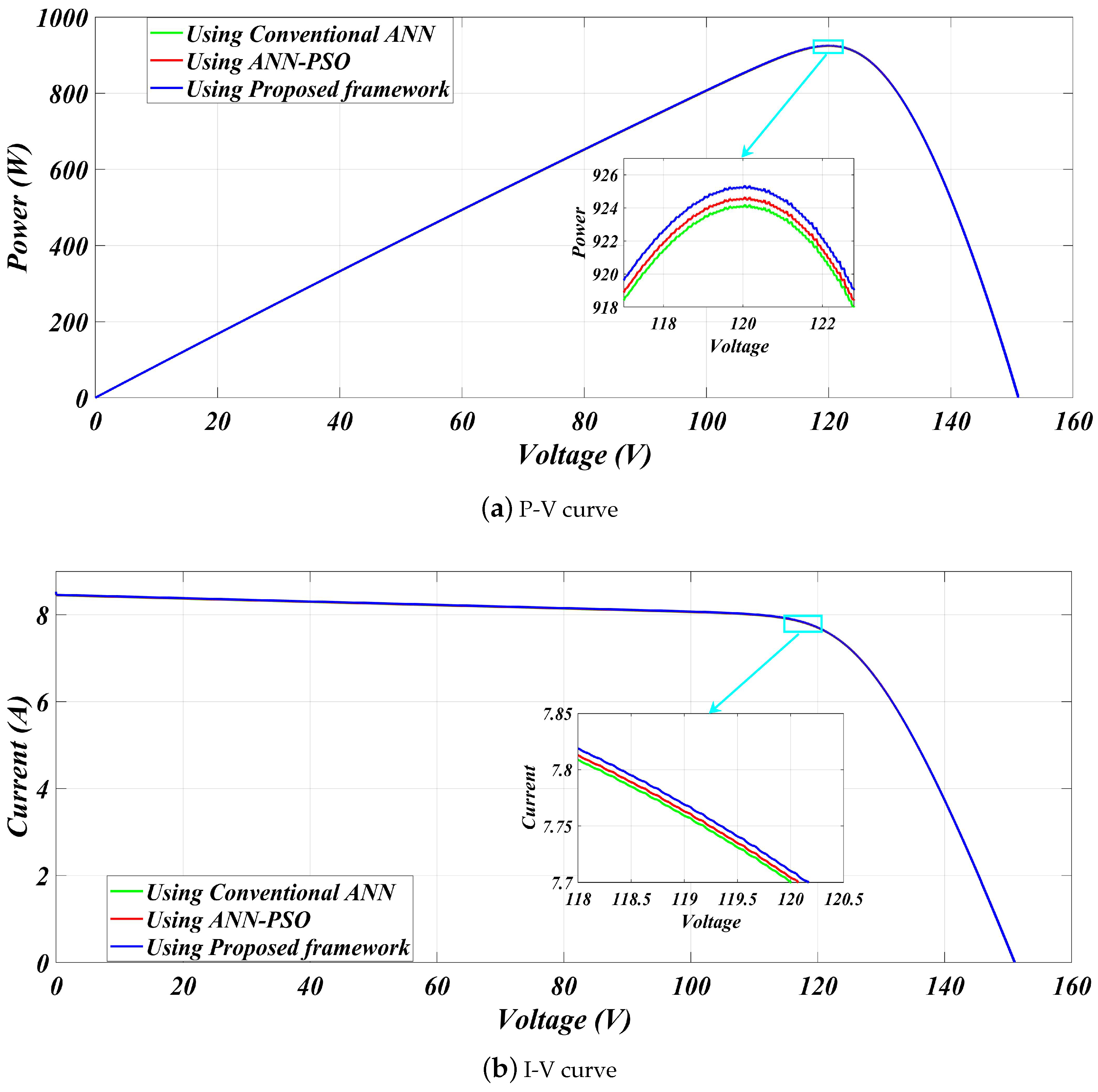
| 1000 | Using Conventional ANN [14] | 925.2 | 924 | 119.9 | 0.00129 | 99.87 |
| Using ANN-PSO [14] | 925.2 | 924.60 | 119.8 | 0.00064 | 99.93 | |
| Proposed framework | 925.2 | 925.09 | 120.02 | 0.00011 | 99.98 | |
| 200 | Using Conventional ANN [14] | 198.9 | 193.12 | 126.8 | 0.02905 | 97.09 |
| Using ANN-PSO [14] | 198.9 | 192.98 | 126.9 | 0.02976 | 97.02 | |
| Proposed framework | 198.9 | 195.70 | 127.2 | 0.01608 | 98.39 |
| Frameworks/Parameters | MSE | Epoch | MPP Tracking Time (s) | Oscillations |
|---|---|---|---|---|
| Proposed | 0.00000409 | 04 | 0.049 | Low |
| ANN-PSO [14] | 0.00068 | 17 | 0.06 | Low |
| Conventional ANN [14] | 0.0079 | 68 | 0.08 | High |
| Irradiance (G) | Frameworks | ΔP (W) | ΔT (s) | 1/ΔT (Hz) | ΔP/ΔT (W/s) |
|---|---|---|---|---|---|
| 200 | Proposed | 0.02076 | 0.02111 | 47.38210 | 0.98402 |
| ANN-PSO [14] | 0.05051 | 0.02585 | 38.68170 | 1.95400 | |
| Conv-ANN [14] | 0.06510 | 0.02588 | 38.62790 | 2.51500 | |
| 1000 | Proposed | 0.01930 | 0.02011 | 49.82800 | 0.96402 |
| ANN-PSO [14] | 0.05239 | 0.03098 | 32.27700 | 1.69100 | |
| Conv-ANN [14] | 0.13830 | 0.03205 | 31.19500 | 4.31500 |
| Cases/Parameters | PMPP (W) | PCalculated (W) | VCalculated (V) | VBoost (V) | MPPEfficiency (%) | MPP Tracking Time (s) |
|---|---|---|---|---|---|---|
| Case-A | 630.21 | 630.20 | 69.15 | 204.5 | 99.99 | 0.08 |
| Case-B | 486.30 | 486.20 | 130.10 | 222 | 99.97 | 0.11 |
| Case-C | 565.32 | 565.30 | 103.20 | 224 | 99.99 | 0.1 |
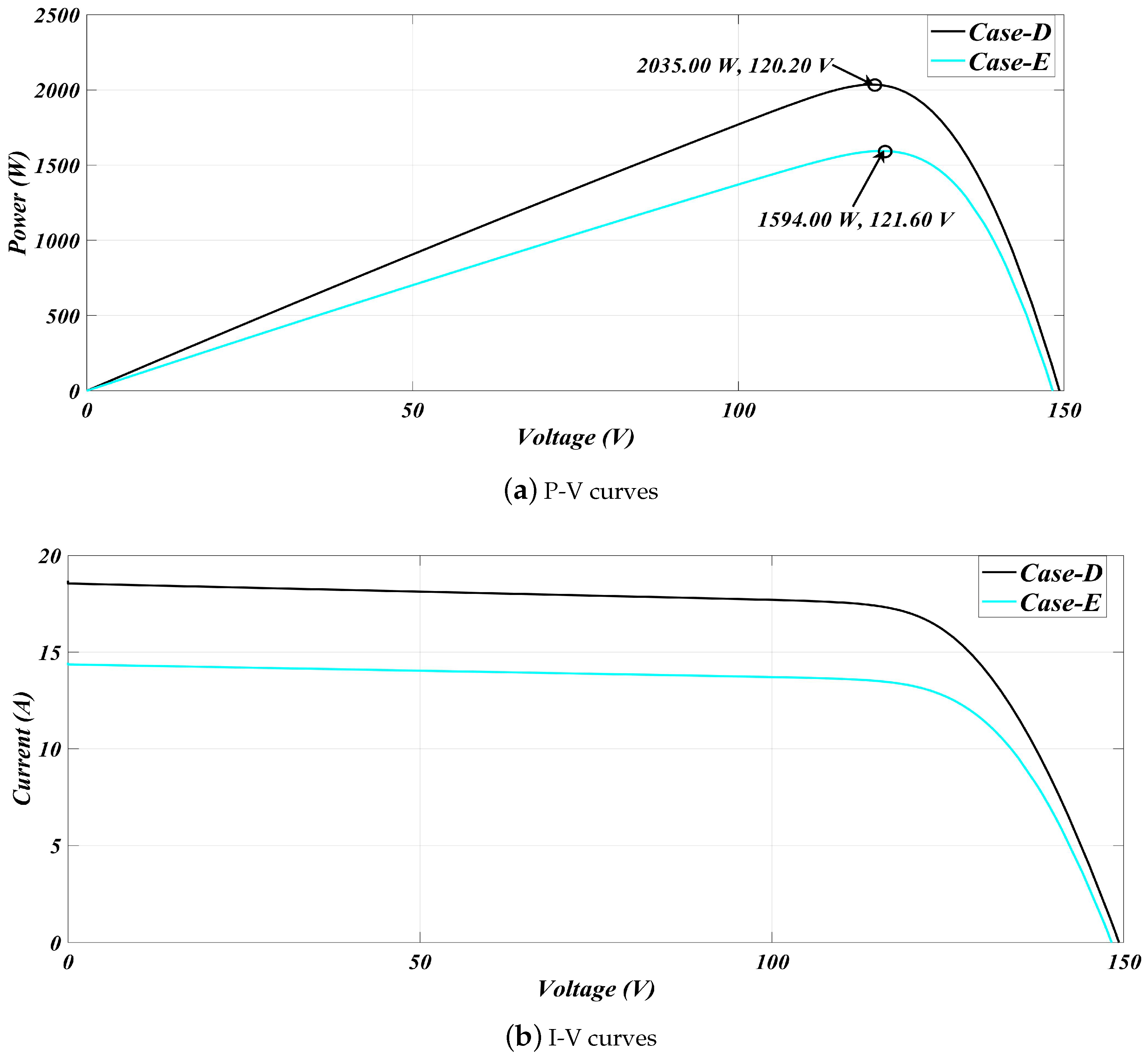
| Case-D | 2035.2 | 2035 | 120.20 | 225 | 99.99 | 0.14 |
| Case-E | 1594.8 | 1594 | 121.60 | 221 | 99.94 | 0.2 |
| Cases/Parameters | PMPP (W) | PCalculated (W) | VCalculated (V) | VBoost (V) | MPPEfficiency (%) | MPP Tracking Time (s) |
|---|---|---|---|---|---|---|
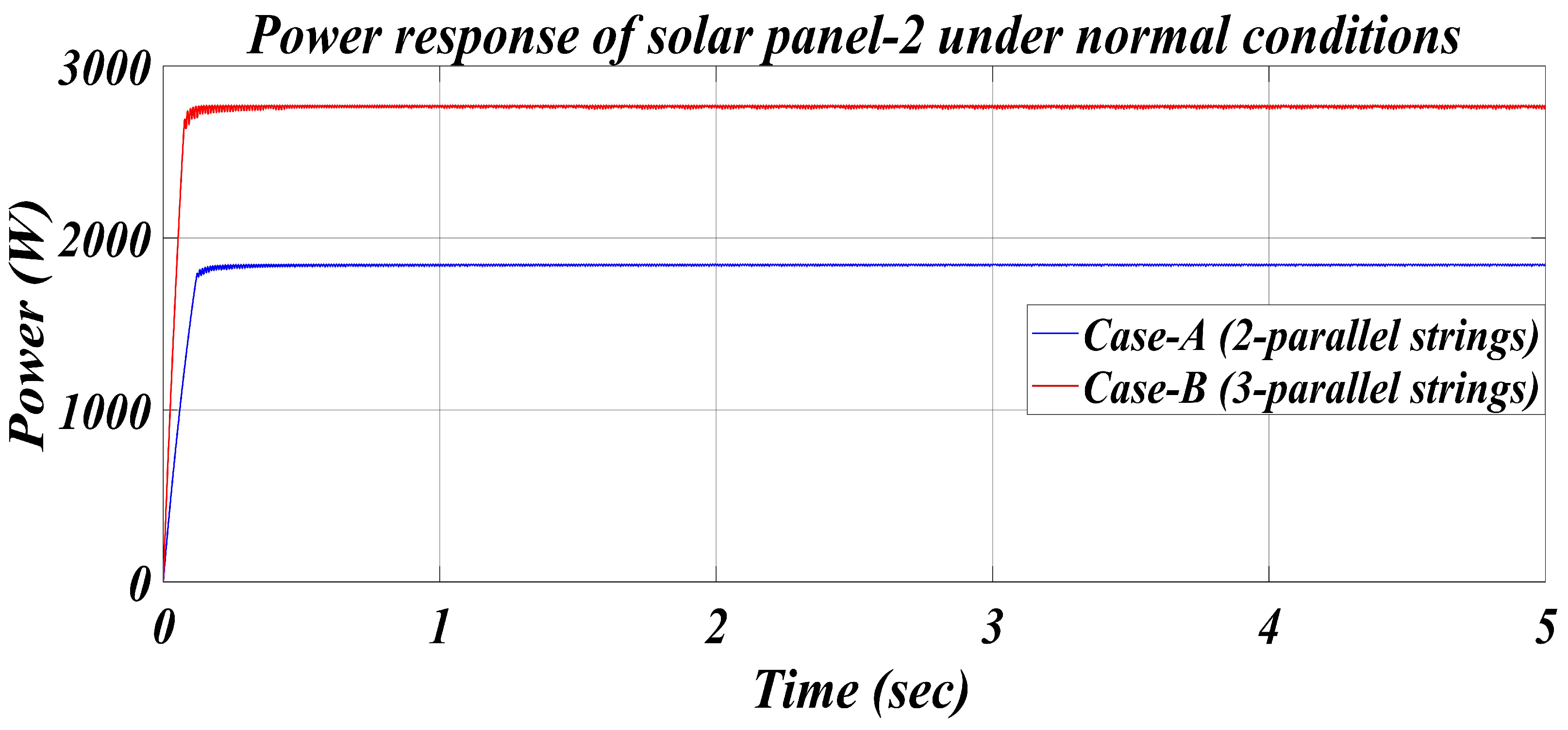
| Case-A | 1850.2 | 1849.8 | 119.9 | 220 | 99.97 | 0.15 |
| Case-B | 2775.6 | 2774.8 | 120.2 | 225 | 99.97 | 0.12 |
Disclaimer/Publisher’s Note: The statements, opinions and data contained in all publications are solely those of the individual author(s) and contributor(s) and not of MDPI and/or the editor(s). MDPI and/or the editor(s) disclaim responsibility for any injury to people or property resulting from any ideas, methods, instructions or products referred to in the content. |
© 2025 by the authors. Licensee MDPI, Basel, Switzerland. This article is an open access article distributed under the terms and conditions of the Creative Commons Attribution (CC BY) license (https://creativecommons.org/licenses/by/4.0/).
Share and Cite
Bisht, R.; Sikander, A.; Sharma, A.; Abidi, K.; Saifuddin, M.R.; Lee, S.S. A New Hybrid Framework for the MPPT of Solar PV Systems Under Partial Shaded Scenarios. Sustainability 2025, 17, 5285. https://doi.org/10.3390/su17125285
Bisht R, Sikander A, Sharma A, Abidi K, Saifuddin MR, Lee SS. A New Hybrid Framework for the MPPT of Solar PV Systems Under Partial Shaded Scenarios. Sustainability. 2025; 17(12):5285. https://doi.org/10.3390/su17125285
Chicago/Turabian StyleBisht, Rahul, Afzal Sikander, Anurag Sharma, Khalid Abidi, Muhammad Ramadan Saifuddin, and Sze Sing Lee. 2025. "A New Hybrid Framework for the MPPT of Solar PV Systems Under Partial Shaded Scenarios" Sustainability 17, no. 12: 5285. https://doi.org/10.3390/su17125285
APA StyleBisht, R., Sikander, A., Sharma, A., Abidi, K., Saifuddin, M. R., & Lee, S. S. (2025). A New Hybrid Framework for the MPPT of Solar PV Systems Under Partial Shaded Scenarios. Sustainability, 17(12), 5285. https://doi.org/10.3390/su17125285