Article

Optimal Multi-Period Manufacturing–Remanufacturing–Transport Planning in Carbon Conscious Supply Chain: An Approach Based on Prediction and Optimization

Laboratoire de Génie Informatique, de Production et de Maintenance, Université de Loraine, 54000 Nancy, France
*
Author to whom correspondence should be addressed.
Sustainability 2025, 17(11), 5218; https://doi.org/10.3390/su17115218
Submission received: 2 April 2025 / Revised: 23 May 2025 / Accepted: 27 May 2025 / Published: 5 June 2025
(This article belongs to the Special Issue Optimization of Sustainable Transport Process Networks)

Abstract

:
This paper presents a joint optimization framework for multi-period planning in a Manufacturing–Remanufacturing–Transport Supply Chain (MRTSC), focusing on carbon emission reduction and economic efficiency. A novel Mixed Integer Linear Programming (MILP) model is developed to coordinate procurement, production, remanufacturing, transportation, and returns under environmental constraints, aligned with carbon tax policies and the Paris Agreement. To address uncertainty in future demand and the number of returned used products (NRUP), a two-stage approach combining forecasting and optimization is applied. Among several predictive methods evaluated, a hybrid SARIMA/VAR model is selected for its accuracy. The MILP model, implemented in CPLEX, generates optimal decisions based on these forecasts. A case study demonstrates notable improvements in cost efficiency and emission reduction over traditional approaches. The results show that the proposed model consistently maintained strong service levels through flexible planning and responsive transport scheduling, minimizing both unmet demand and inventory excesses throughout the planning horizon. Additionally, the findings indicate that carbon taxation caused a sharp drop in profit with only limited emission reductions, highlighting the need for parallel support for cleaner technologies and more integrated sustainability strategies. The analysis further reveals a clear trade-off between emission reduction and operational performance, as stricter carbon limits lead to lower profitability and service levels despite environmental gains.

1. Introduction

In recent years, the conversation around sustainability has shifted from aspirational goals to urgent imperatives. As global environmental concerns grow sharper, companies are under increasing pressure to adopt responsible practices that not only minimize ecological harm but also ensure long-term economic resilience. Among the most critical avenues for achieving this balance is the supply chain, a complex system that, when managed thoughtfully, can serve as both a driver of sustainability and a source of competitive advantage. A truly sustainable supply chain is not merely about reducing emissions; it is about rethinking how resources are used, how waste is handled, and how products can have a second life through recovery and reuse [1]. This transformation begins with two foundational pillars: reverse logistics and remanufacturing. By facilitating the return, recovery, and regeneration of products, these practices help close the loop of production and consumption. Their value, however, goes beyond environmental benefit; they also reduce raw material dependency and offer measurable economic returns [2]. Yet, sustainability in the supply chain cannot be achieved by these practices alone. Transportation, the lifeblood of logistics, plays a central role in determining the environmental footprint of supply chain operations. Optimizing routes, upgrading fleets to low-emission alternatives, and making smarter modal choices are all essential to reducing greenhouse gas emissions and improving efficiency [3]. Despite its importance, transportation remains an often-underexplored element in sustainability research. Equally important is the regulatory landscape, which continues to evolve with policies aimed at capping emissions and encouraging greener practices. From carbon pricing to mandatory reporting systems, these mechanisms are shaping corporate behavior and pushing innovation in sustainable operations. To navigate this complex terrain, companies must move beyond piecemeal solutions. They require integrated, data-driven strategies, such as joint optimization frameworks, that consider production, transportation, inventory, and emissions simultaneously. Recent research in this domain has underscored the importance of such holistic approaches, highlighting their potential to reconcile environmental responsibility with operational excellence. It is within this context that the present study situates itself. By examining the interplay between logistics, regulation, and predictive planning, and by leveraging advanced modeling tools, this work contributes to the ongoing effort to build supply chains that are not only efficient but also aligned with the broader goals of sustainability and climate responsibility.
This document is structured as follows: Section 2 reviews the relevant literature. Section 3 highlights the specific contributions of the study. Section 4 introduces the proposed system and outlines the problem being addressed. Section 5 details the formulation and development of the mathematical model, incorporating the underlying assumptions. Section 6 provides a comparative study to identify the best prediction algorithm and numerical examples to illustrate the applicability of the proposed approach. Section 7 is devoted to the numerical results and the discussion of the main findings. Finally, Section 8 concludes the paper and outlines potential directions for future research.

2. Literature Review

To establish a comprehensive sustainable supply chain, integrating practices such as reverse logistics and remanufacturing is crucial, as they both address environmental and economic challenges [4]. Reverse logistics involves the efficient return and recovery of products, facilitating reuse, recycling, or proper disposal, thereby minimizing waste [5]. Remanufacturing complements this by restoring used products to like-new condition, extending their lifecycle and reducing the demand for raw materials. Recent studies highlight the significance of these practices in promoting a circular economy. For instance, ref. [6] emphasize the role of remanufacturing in value retention of waste products, while [7] discuss simplifying reverse logistics to enable remanufacturing in the automotive sector. Collectively, these approaches not only mitigate environmental impacts but also offer cost-saving opportunities, aligning business operations with global sustainability objectives [8].
Achieving a truly comprehensive sustainable supply chain requires addressing all critical components, including reverse logistics, remanufacturing, and transportation activities, as transportation significantly impacts environmental performance and operational efficiency. Strategies such as adopting low-emission vehicles, alternative fuels, and optimized routing are essential for reducing greenhouse gas emissions [9]. Decisions on transportation modes, vehicle types, and routing further decrease environmental impact [10]. Despite its importance, transportation activities receive limited attention in sustainable supply chain research, though they are vital for real-world efficiency. Recent studies, such as [9,11], highlight models addressing emissions and multi-stage transportation challenges within sustainability frameworks.
Reducing the carbon footprint is a critical objective in the pursuit of sustainable development, particularly within supply chains where emissions are significant contributors to climate change. Key strategies, such as adopting energy-efficient technologies and optimizing logistics to minimize transportation-related emissions, enable organizations to address environmental challenges while improving operational efficiency and aligning with global sustainability goals. These carbon reduction efforts are closely tied to compliance with emission regulation policies, which play a vital role in mitigating climate change by setting strict limits on greenhouse gas emissions [12]. Such policies, including carbon pricing, emissions trading systems, and mandatory reporting requirements, incentivize the adoption of sustainable practices across industries [13]. Additionally, by promoting renewable energy, energy-efficient technologies, and low-carbon transportation options, these regulations not only reduce emissions but also drive innovation and long-term sustainability [14].
Achieving sustainable supply chains requires integrating carbon reduction strategies and regulatory compliance with advanced joint optimization approaches to address emissions holistically [15]. In this context, joint optimization in a low-carbon sustainable supply chain focuses on integrating multiple decision-making processes across various stages to simultaneously minimize carbon emissions and enhance operational efficiency. This approach encompasses the coordinated optimization of transportation, inventory management, and production scheduling while aligning with carbon reduction targets. Recent research has advanced the understanding of these strategies by developing innovative models to balance environmental and economic outcomes.
For example, ref. [16] proposed a multi-objective optimization model for a joint enterprise supply chain, demonstrating that collaborative approaches significantly improve both environmental performance and economic efficiency. Similarly, ref. [17] explored low-carbon closed-loop supply chain strategies using differential games, emphasizing the effectiveness of dynamic optimization in managing new and remanufactured products. Additionally, ref. [18] presents a robust optimization model aimed at supporting green supplier selection and order allocation decisions within a closed-loop supply chain framework under the cap-and-trade mechanism, further showcasing the benefits of collaborative strategies in achieving carbon reduction and operational efficiency. In the same context [19], introduced a novel control model for managing unreliable manufacturing and remanufacturing systems, integrating environmental subsidies and overrun penalties to optimize production decisions. The model aims to balance economic performance with environmental considerations, providing a framework for sustainable operations. Collectively, these studies highlight the critical role of joint optimization in designing low-carbon supply chains that align with sustainability objectives and regulatory requirements.
While the studies reviewed above provide valuable insights into collaborative strategies, game-theoretic models, and green optimization under cap-and-trade or subsidy mechanisms, they often consider partial segments of the supply chain or rely on simplified assumptions such as unlimited inventory or indistinguishable product types. In contrast, our proposed framework addresses the supply chain as a fully integrated system, from raw material procurement to returns, while explicitly accounting for real-world constraints such as limited buffer stocks and differentiated pricing between new and remanufactured products. Unlike the models existing in the literature, which emphasize conceptual optimization or policy modeling, our work brings a practical and data-driven perspective by embedding demand and return forecasting into the decision-making process. The integration of a predictive layer with the MILP model enhances the realism and planning accuracy of the system, especially in dynamic environments. Furthermore, by incorporating contract carrier logistics and carbon tax mechanisms, we move beyond static optimization toward a more actionable, operations-oriented approach. This positions our contribution as both complementary to, and more practically grounded than, existing models, especially in terms of implementation readiness and alignment.
As it is known, multi-period planning in the supply chain framework involves determining future decisions regarding production, inventory, transportation, etc. [20]. Moreover, achieving efficient planning requires not only a robust model but also meaningful input data that may reflect real case or logic values in one domain. To achieve this target, we will estimate the future values of both demand and NRUP using a predictive model. These estimates will then be used as input data for the developed MILP to determine the optimal plan. Indeed, machine learning and predictive modeling play a crucial role in estimating future values, thereby enhancing supply chain efficiency. These models offer valuable insights into demand fluctuations and operational variables, enabling organizations to make data-driven decisions. The prediction approaches that are used in logistics provide insight into future demands and events to better manage supply and meet customer needs. Research in industrial and logistic fields typically provides input data in the form of averages or stochastic processes inspired by historical records [21]. Predictive models estimate future values while accounting for variability and seasonality, as well as capturing the interdependence between different events or phenomena. That provides meaningful values in relation to the industrial practice, which the planning management relies on to make optimal decisions. Among these predictive models in the literature, we found Vector AutoRegression (VAR), Seasonal AutoRegressive Integrated Moving Average (SARIMA), Long Short-Term Memory (LSTM), SARIMA/VAR hybrid, Holt–Winters Exponential Smoothing (HWES), and Ridge Regression Model (RRM).
The VAR model [22] is well-suited for modeling multivariate time series and capturing interdependencies among variables. It takes into account how past values of all variables influence one another, making it valuable for multivariate forecasting. The model incorporates delayed effects between variables, which is crucial when changes in one series impact another with a time lag. Consequently, the VAR model can predict all series simultaneously while considering their mutual influences. Ref. [23] have used a VAR model to predict the energy demands and compared it to the LSTM model with respect to three datasets of household energy management systems. The SARIMA is an extension of the Auto-Regressive Integrated Moving Average model [24], a specialized time-series model that combines elements of seasonality and exponential smoothing techniques. It is particularly useful for handling seasonal patterns in data while incorporating both autoregressive and moving average components, along with exponential smoothing for better adaptability. It is particularly useful for analyzing time-series data with periodic patterns, such as monthly, quarterly, or yearly trends. SARIMA is defined by its parameters for both non-seasonal (p, d, q) and seasonal (P, D, Q, s) components. Ref. [25] have used the SARIMA model to forecast demand patterns in the context of e-commerce. Ref. [26] used SARIMA to forecast future demand based on data spanning over 37 months of actual retail sales. Compared to LSTM, they demonstrated that SARIMA yields better results for products with seasonal behavior, whereas LSTM performs better for products with stable demand. Indeed, LSTM [27] is a specialized form of recurrent neural networks designed to model long-term dependencies in sequential data. Effectively, it captures nonlinear relationships and processes both univariate and multivariate time series. It is characterized by a flexible number of units (neurons) per layer and network depth, balancing computational complexity and learning capacity. Ref. [28] used an LSTM model to predict demand for humanitarian logistics in a complex problem considering immediate real implications. The model is reliable for forecasting but requires a large amount of training data. Another model, known as the SARIMA/VAR hybrid model, combines SARIMA and VAR to integrate both univariate components (trend/seasonality) and multivariate dependencies. It effectively captures univariate patterns (trend/seasonality) as well as multivariate relationships, making it more robust than standalone SARIMA or VAR. Although this hybrid model is robust, it is rarely used in literature due to its complexity in implementation. Addressing this limitation is one of the contributions of our work. The HWES [29] is a time-series forecasting method that adjusts parameters dynamically to capture level, trend, and seasonality. It provides optimal predictions by fine-tuning smoothing coefficients to reflect changes in demand and operational patterns. Finally, the RRM [30] is a regression-based predictive model that incorporates Ridge regularization to prevent overfitting. It is useful for handling multi collinear data while ensuring stable and interpretable parameter estimates. In conclusion, we will select some predictive models from the literature according to the data analysis and then find the optimal prediction.

3. Targeted Contributions

This study presents several key contributions to the field of sustainable supply chain optimization. First, we prioritize raw material procurement as a fundamental consideration in system design, ensuring a more efficient and resilient supply chain. Unlike many existing studies that focus on isolated components, we propose a comprehensive full supply chain system that integrates raw material ordering, manufacturing, remanufacturing, shipping, and return logistics within a real-world operational framework. To optimize decision-making across this integrated system, we develop a mixed-integer linear programming (MILP) model, which simultaneously determines optimal raw material procurement, transportation, remanufacturing, manufacturing, and return plans to maximize overall profitability. Another significant contribution is addressing the gap in the literature concerning pricing and quality differentiation between new and remanufactured products. While prior research often assumes these products are indistinguishable and share the same market price, we introduce a more realistic approach by distinguishing them based on their quality and pricing structure. Additionally, we incorporate contract carriers for transportation, acknowledging their role in improving operational efficiency, reducing costs, and enhancing service reliability. This integration ensures a more practical representation of supply chain dynamics, particularly in urban distribution systems. Unlike previous models that assume infinite inventory capacity and continuous machine operation, our study considers real-world constraints, including finite buffer stocks in both upstream and downstream stages. Moreover, we integrate carbon tax policy as a carbon reduction strategy while jointly optimizing various stages of the supply chain, aligning our model with global sustainability objectives. Collectively, these contributions enhance the realism, efficiency, and sustainability of supply chain decision-making, providing a robust framework for optimizing economic and environmental performance in low-carbon supply chains. Another major contribution involves forecasting future values of demands and NRUP using prediction models, which are then utilized by the MILP to provide efficient joint planning in line with practical applications. The challenge of this contribution lies in implementing various predictive models and selecting the best one while considering the interdependencies between the parameters

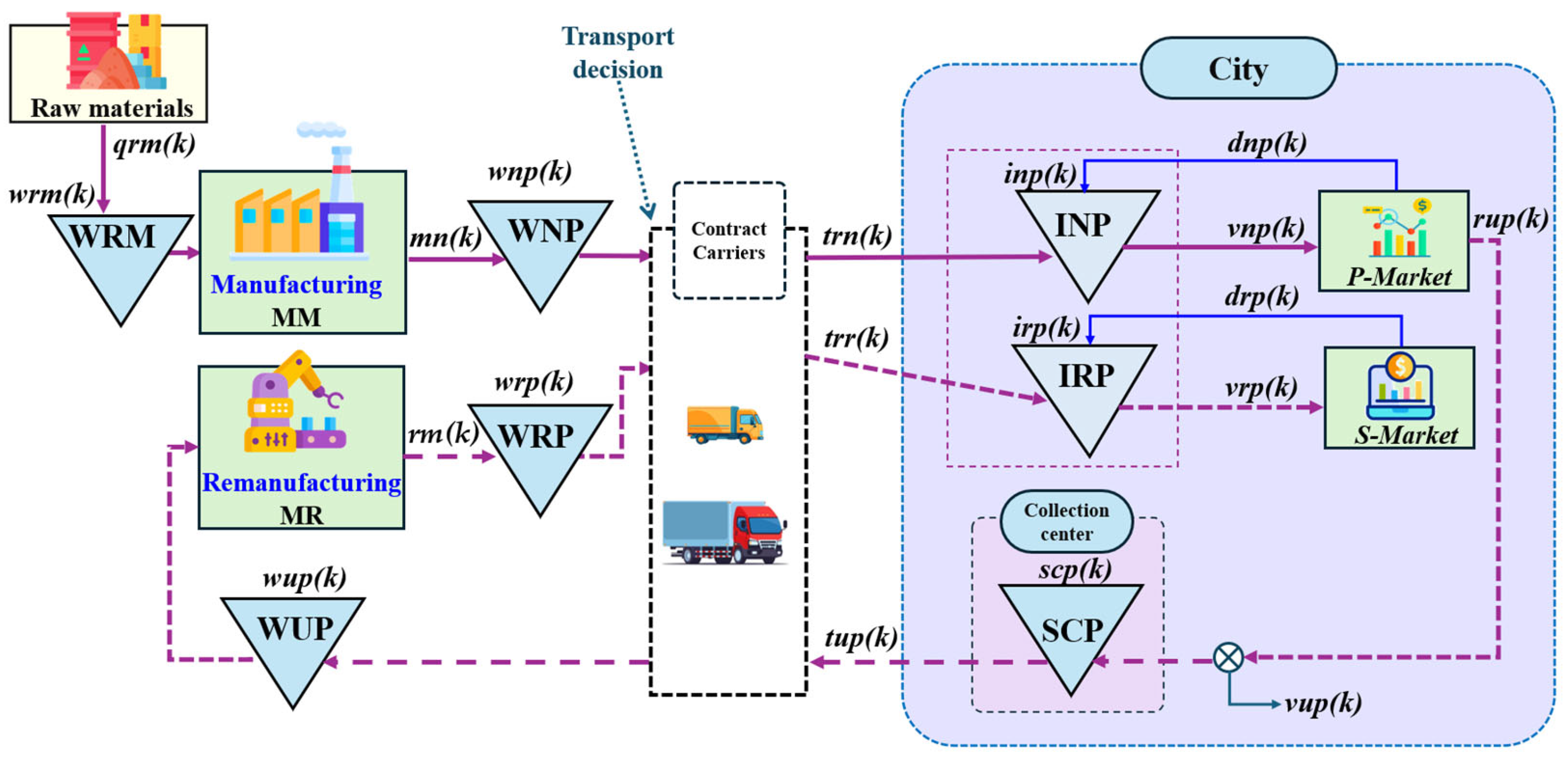
4. Problem Statement

This section presents and explains the suggested system (refer to Figure 1). Within the factory, the manufacturing of new products using raw materials is processed by the machine MM. These products are sold later to the primary market P-Market located in the city. However, the machine MR processes the remanufacturing of products using end-of-life returned items. These products are sold later to the secondary market S-Market located in the same city. The sales inventories INP and IRP satisfy consumers’ constant demands for manufactured dnp(k) and remanufactured drp(k) products at every period k. Taking into consideration the limited capacities of the inventory’s stocks as well as the upstream and downstream buffer stocks, the warehouse raw material stock WRM fills the machine MM, and the warehouse used products stock WUP fills the machine MR. Within the city, the returned used products will be stocked in SCP (stock of collected products) with consideration of its capacity. The excess quantity of collected products, vup(k), will be set aside for sale at a later time.
The city will receive the outgoing quantities trn(k) from the warehouse of new products stock WNP and trr(k) from the warehouse of returned products WRP. The transportation activities will be provided by two different vehicles with different capacities (contract carriers) dependent on the transport decision. There are two sales inventories for new and remanufactured products next to each other, defined as INP and IRP, respectively. The values vpn(k) and vrp(k), respectively, indicate the quantities of new and remanufactured products sold at period k. In preparation for remanufacturing, the quantities of end-of-life used products rup(k) will be collected and stored in stock SCP. Production is scheduled into equal-length production intervals across a defined horizon. The goal is to maximize profit, which is calculated as follows: profit is defined as total revenue from sales of new and remanufactured items and sales of exceeded quantities of collected items less total expected cost throughout the production planning horizon. This cost consists of production costs as well as inventory holding costs, costs associated with shortages, transportation costs, acquisition costs, costs associated with returning products, and an extra cost for carbon emissions.

5. Analytical Study

5.1. Notations

The parameters and decision variables that are used in this work to define the model and describe the problem are listed below.

5.1.1. Parameters

The following are parameters.
λLength of the production period
ZNumber of production periods in the planning horizon
Z. λLength of the finite planning horizon
PRCX(Z)Total profit considering carbon tax strategy
qrm(k)Quantity of raw materials to order during period k
qrm0Quantity of raw materials to order at the start of period 1
mn(k)Produced quantity of machine MM during period k
mn0Produced quantity of machine MM at the start of period 1
rm(k)Produced quantity of machine MR during period k
rm0Produced quantity of machine MR at the start of period 1
trn(k)Transported quantities of new products at period k
trn0Transported quantities of new products at the start of period 1
trr(k)Transported quantities of remanufactured products at period k
trr0Transported quantities of remanufactured products at the start of period 1
tup(k)Transported used products from SCP to WUP at period k
tup0Transported used products from SCP to WUP at the start of period 1
rup(k)Quantity of collected used products from the primary market at period k
rup0Quantity of collected used products from the primary market at the start of period 1
vup(k)Quantity sold of collected products at the end of period k
vup0Quantity sold of collected products at the start of period 1
wrm(k)Warehouse level of raw materials at the end of period k
wrm0Warehouse level of raw materials at the start of period 1
wnp(k)Warehouse level of new products at the end of period k
wnp0Warehouse level of new products at the start of period 1
wrp(k)Warehouse level of remanufactured products at the end of period k
wrp0Warehouse level of remanufactured products at the start of period 1
wup(k)Warehouse level of used products at the end of period k
wup0Warehouse level of used products at the start of period 1
inp(k)Sales inventory level of new products at the end of period k
inp0Sales inventory level of new products at the start of period 1
irp(k)Sale inventory level of remanufactured products at the end of period k
irp0Sale inventory level of remanufactured products at the start of period 1
scp(k)Storage level of collected used products in SCP at the end of period k
scp0Storage level of collected used products in SCP at the start of period 1
dnp(k)Demand in the primary market (new product) at the period k
drp(k)Demand in the secondary market (remanufactured product) at the period k
lnp (k)Unsatisfied demand quantity of new products at the period k
lnp0Unsatisfied demand for new products at the start of period 1
lrp (k)Unsatisfied demand quantity of remanufactured products at the period k
lrp0Unsatisfied demand quantity of remanufactured products at the start of period 1
xCost acquisition of one raw materials unit
aUnit production cost of new products
bUnit production cost of remanufactured products
wxWarehousing cost of one raw materials unit in WRM
waWarehousing cost of one new product in WNP
wbWarehousing cost of one remanufactured product in WRP
wcWarehousing cost of one remanufactured product in WUP
ctTransport cost of new product
caInventory holding cost of one new product in INP
cbInventory holding cost of one remanufactured product in IRP
csStorage cost of one collected item unit in SCP
yCost of one returned product
snShortage cost of one new product
srShortage cost of one remanufactured product
FT1Fixed round trip cost for vehicle V1
FT2Fixed round trip cost for vehicle V2
TCX (Z)Total carbon tax cost over the horizon
vnp(k)Quantity of new products sold at period k
vnp0Quantity of new products sold at the start of period 1
vrp(k)Quantity of remanufactured products sold at period k
vrp0Quantity of remanufactured products sold at the start of period 1
pnUnit selling price for a new product
prUnit selling price for remanufactured product
pvUnit selling price for collected product
ucpUnit carbon tax price
CF(Z)Carbon footprint over Z
CF0Carbon footprint at the start of period 1
RMMaximum capacity of WRM
NPMaximum capacity of WNP
RPMaximum capacity of WRP
NMaximum capacity of INP
RMaximum capacity of IRP
SPMaximum capacity of SCP
TRV1Capacity of the transport vehicle V1
TRV2Capacity of the transport vehicle V2
γ1(k)Transport decision variable for the vehicle 1
γ2(k)Transport decision variable for the vehicle 2
BNBig number for the linearization
GMMaximum quantity produced by MM during period k
GRMaximum quantity produced by MR during period k
emUnit carbon emissions from acquisition of raw materials
enUnit carbon emissions from manufacturing new product
erUnit carbon emissions from remanufacturing product
ermUnit carbon emissions from holding raw materials in WRM
ewnUnit carbon emissions from holding new product in WNP
ewrUnit carbon emissions from holding remanufactured in WRP
escUnit carbon emissions from holding one collected product in SCP
ecuUnit carbon emissions from holding one used product in WUP
enpUnit carbon emissions from holding new product in INP
erpUnit carbon emissions from holding remanufactured products in IRP
etrUnit carbon emissions from transporting new, remanufactured, or returned products
efrt1Fixed quantity of carbon emitted by vehicle V1
efrt2Fixed quantity of carbon emitted by vehicle V2
MC(Z)Manufacturing cost over Z
RC(Z)Remanufacturing cost over Z
NSC(Z)Shortage cost of new products over horizon Z
RSC(Z) Shortage cost of remanufactured products over horizon Z
HRM(Z)Inventory holding cost of raw material stock over horizon Z
HNP(Z)Inventory holding cost of new products stock over horizon Z
HRP(Z)Inventory holding cost of remanufactured products stock over horizon Z
HUP(Z)Inventory holding cost of returned products stock over horizon Z
HIN(Z)Inventory holding cost of sales inventory stock of new products over horizon Z
HIR(Z)Inventory holding cost of sales inventory stock of remanufactured products over horizon Z
HCP(Z)Inventory holding cost of stock of collected products over horizon Z
TC(Z)Transportation cost over horizon Z
ARM(Z)Acquisition of raw material cost over horizon Z
RPC(Z)Returned products cost over horizon Z
R(Z)Revenue over the horizon Z

5.1.2. Decision Variables

The following is how the different decision variables are presented.
QRMraw materials quantity order plan
MNmanufacturing plan of the machine MM
RMremanufacturing plan of the machine MR
TRNtransport plan of new products
TRRtransport plan of remanufactured products
TUPtransported returned quantity plan of used products from SCP
In order to maximize the total profit PRCX(Z), we determine the optimum values of the decision variables QRM*, MN*, RM*, TRN*, TRR*, and TUP* in this study. As a result, the maximum (optimal) value of PRCX(Z) is equal to the value of PRCX*(Z).
The problem of mixed-integer linear programming corresponds to the profit model that must be developed under constraints related to production, acquisition, inventory, transport, and carbon emissions.

5.2. Working Assumptions

We consider the following assumptions in the section that follows:
  • We assume that after their useful lives are over, the remanufactured products sold in Market 2 will be destroyed;
  • We assumed that the demands dnp(k), drp(k), and rup(k) are predicted using best prediction model;
  • To meet the demands dnp(k) and drp(k), the quantities mn(k) and rm(k) produced during period k are added to the stock at the end of the period;
  • There are no backorders, and a shortage cost is incurred because the units are lost;
  • Considering that the remanufactured products were the same size as the new ones but were of lower quality and price;
  • It is assumed that stocks WRM, WNP, WRP, INP, IRP, and SCP have limited capacities;
  • We consider the period of time between the making of an order and the reception of raw materials. It means that the decided quantity of raw materials is ordered at period k and received at time k+ 1 in order to have a realistic approach to our system.

5.3. Formulation of the Total Expected Profit

We began by creating equations and constraints related to inventory balance, production capacity, transport capacity, the number of new and used products sold at a given time, and carbon emissions. This helped us estimate the total cost for the whole planning period.

5.3.1. Balance Inventory

Equations (1) and (2) describe the evolution of new product inventory in the warehouse over time. Specifically, Equation (1) models the inventory balance at the end of each period k + 1, denoted as wnp(k + 1), based on three elements: the remaining inventory from the previous period wnp(k), the number of newly produced units mn(k + 1), and the quantity transported out for sales or distribution trn(k + 1). This relationship ensures that the warehouse inventory reflects actual operational activity: what is produced adds to the stock, and what is shipped reduces it. Equation (2) defines the initial condition at period 1. Here, the starting warehouse level wnp(1) is determined by the initial inventory wnp0, the quantity produced mn(1), and the transported quantity trn(1).
These equations are essential for maintaining an accurate flow of inventory throughout the system, ensuring that warehouse levels remain consistent with production outputs and logistics operations over the entire planning horizon.
w n p k   + 1 =   w n p k +   m n k   + 1 t r n k   + 1         k   = 0 ,   ,   Z 1
w n p 1 = w n p 0 +   m n 1 t r n 1  
Equations (3) and (4) describe how the remanufactured product inventory in the warehouse evolves over time. In Equation (3), the inventory level at the end of each period k + 1, denoted wrp(k + 1), is determined by the inventory carried over from the previous period wrp(k), the quantity of remanufactured products produced during the current period rm(k + 1), and the quantity transported out for distribution or sales trr(k + 1). This formulation captures the fundamental inventory balance: what is produced adds to stock, while what is shipped out reduces it.
Equation (4) sets the initial warehouse level for remanufactured products at the end of period 1. It combines the initial stock wrp0, the production volume rm(1), and the transported amount trr(1) to determine the available inventory at that point.
Together, these equations allow the model to track the flow of remanufactured products across the planning horizon, ensuring consistency between production, storage, and outbound logistics in the reverse side of the supply chain.
w r p k   + 1 =   w r p k +   r m k   + 1 t r r k   + 1     k   = 0 ,   ,   Z 1
w r p 1 = w r p 0 +   r m 1 t r r 1  
Equations (5) and (6) describe the inventory flow of collected used products within the storage facility SCP over time. Specifically, Equation (5) updates the storage level at the end of each period k + 1 by adding the quantity of newly collected used products from the market rup(k + 1), and subtracting the quantity transported to the remanufacturing facility tup(k + 1). This balance ensures that the storage level reflects both incoming and outgoing flows at each time step.
Equation (6) sets the initial condition for this dynamic, defining the stock level at the end of period 1 as a function of the initial stored quantity scp0, the used products collected at the start rup(1), and the number transported for processing tup(1).
Together, these equations enable the model to accurately track the availability of used products within the reverse logistics system across all planning periods k = 0, , Z − 1, and account for fluctuations in both return volumes and remanufacturing throughput. They are particularly important for capturing the real-time behavior of a sustainable supply chain that integrates product returns, temporary storage, and remanufacturing flows.
s c p ( k + 1 ) =   s c p ( k ) +   r u p ( k   + 1 ) t u p ( k   + 1 )   k   = 0 ,   ,   Z 1
s c p k =   s c p 0 + r u p 1 t u p ( 1 )
As previously discussed in the section on working assumptions, we choose to place our raw material order at time k, and we anticipate receiving it in the subsequent period k + 1, once it reaches stock WRM, which has a limited capacity.
Equations (7) and (8) describe the evolution of raw material inventory in the warehouse over the planning horizon. Specifically, Equation (7) calculates the stock level of raw materials at the end of each period k + 1 based on three factors: the stock remaining from the previous period wrm(k), the quantity of raw materials ordered during the current period qrm(k), and the quantity consumed by the production process mn(k + 1). This equation ensures that material usage for manufacturing is properly reflected in the inventory update, capturing the flow of resources within each cycle.
Equation (8) defines the initial condition for this inventory stream, where the warehouse level at the end of period 1 is determined by the starting stock wrm0, the quantity ordered at the beginning qrm(0), and the materials used by the machine mn(1).
Together, these equations provide a straightforward yet essential mechanism for tracking raw material availability across all periods k = 0, , Z − 1, ensuring that production decisions remain feasible and aligned with procurement planning. They also establish a clear connection between procurement schedules and production demands, which is crucial for maintaining operational continuity in the system.
w r m ( k   + 1 ) =   w r m ( k ) +   q r m ( k )   m n ( k   + 1 )   k   = 0 , ,   Z 1
w r m ( 1 ) =   w r m 0 +   q r m ( 0 ) m n ( 1 )
Within the structure of the supply chain, INP refers specifically to the inventory location for new products, while IRP holds remanufactured products, each serving the primary and secondary markets, respectively. By clearly separating these two sales inventory streams, the model reflects the practical dynamics of dual-market supply strategies and supports more accurate inventory planning.
Equation (9) governs the inventory flow of new products in the primary sales market, represented by the inventory variable inp(k + 1). This equation ensures that the sales inventory at the end of period k + 1 accounts for three essential elements: the stock carried over from the previous period inp(k), the quantity of new products transported to the sales point during the current period trn(k + 1), and the quantity sold in the same period vnp(k + 1). In essence, the available inventory grows with incoming stock and decreases as sales are fulfilled. This formulation is applied across all planning periods k = 0, , Z − 1, and allows the model to continuously update and monitor inventory levels in response to supply and demand variations.
i n p ( k + 1 ) = i n p ( k ) +   t r n ( k   + 1 ) v n p ( k   + 1 )   k   = 0 ,   ,   Z 1
Equation (10) describes the inventory dynamics of remanufactured products in the secondary sales market. Specifically, irp(k + 1) represents the inventory level at the end of period k + 1, and it is calculated by adding the incoming remanufactured products trr(k + 1) to the existing inventory irp(k), then subtracting the quantity sold during that period vrp(k + 1). This simple yet essential balance ensures that the remanufactured stock is accurately updated across each time step based on actual inflows and outflows.
This relationship holds for all periods k = 0, , Z − 1, and is fundamental to maintaining a reliable supply of remanufactured products in the secondary market.
i r p k   + 1 =   i r p k +   trr ( k + 1 ) v r p k   k   = 0 ,   ,   Z 1
Equations (11) and (12) define two binary decision variables, γ1(k) and γ2(k), which are used to indicate whether a specific transport vehicle is assigned to perform a round-trip during period k. More precisely,
γ 1 ( k ) = 1   i f   v e h i c u l e   1   w i l l   d o   t h e   r o u n d   t r i p 0   o t h e r w i s e  
γ 2 ( k ) = 1   i f   v e h i c u l e   2   w i l l   t h e   r o u n d   t r i p 0   o t h e r w i s e  
These binary indicators are essential for controlling and tracking transportation activities within the supply chain. By explicitly modeling vehicle availability through these variables, the system ensures that logistical constraints are respected, especially in cases where transport capacity, cost, or environmental impact must be factored into the decision-making process. This also allows the model to simulate real-world fleet scheduling more accurately within the broader optimization framework.

5.3.2. Quantities Sold of New and Remanufacturing Products at Period k

Equations (13) and (14) determine the actual sales quantities of new and remanufactured products in each period by accounting for both customer demand and inventory availability. In Equation (13), the quantity of new products sold in period k, denoted as vnp(k), is defined as the minimum between the demand in the primary market dnp(k) and the available inventory from the previous period inp(k − 1). This formulation ensures that sales do not exceed what is physically available in stock, and thus respects inventory constraints.
Similarly, Equation (14) defines the sales of remanufactured products vrp(k) as the minimum of the demand in the secondary market drp(k) and the remanufactured inventory carried over from the previous period irp(k − 1). Again, this guarantees that only the quantity available in inventory can be sold.
Together, these two equations reflect a realistic sales mechanism in both the primary and secondary markets, where product availability may limit fulfillment even when demand exists. By capturing this dependency, the model ensures a more accurate representation of how inventory levels impact service performance across planning periods.
vnp (k) = min (dnp (k), inp(k − 1))
v r p ( k ) = min ( d r p ( k ) , i r p ( k   -   1 ) )
The following subsection represents the total cost incurred over the finite planning horizon Z, encompassing production costs, shortage penalties, inventory holding costs, transportation expenses, raw material procurement, and the handling of returned products. For notational simplicity, we set λ = 1 throughout the formulation.

5.3.3. Manufacturing and Remanufacturing Costs

Equations (15) and (16) define the cumulative manufacturing and remanufacturing costs over the planning horizon Z. In Equation (15), MC(Z) represents the total manufacturing cost of new products, calculated as the product of the unit production cost a and the sum of all new product quantities mn(k) produced over each period k = 1, , Z.
Similarly, Equation (16) defines RC(Z), the total remanufacturing cost, as the unit cost b multiplied by the total volume of remanufactured products rm(k) produced across the same horizon. These two expressions quantify the direct production-related expenses for both product streams, new and remanufactured, and form a key component of the overall cost structure in the supply chain model.
M C ( Z ) = a   × k = 1 Z m n k
R C ( Z ) =   b × k = 1 Z r m k

5.3.4. Shortage Costs

Equations (17)–(20) quantify the shortage costs associated with unmet demand for both new and remanufactured products over the planning horizon Z. Equation (17) defines lnp(k), the unsatisfied demand for new products at period k, as the difference between the actual demand dnp(k) and the quantity fulfilled vnp(k). Similarly, Equation (18) computes the unsatisfied demand for remanufactured products lrp(k), as the gap between demand drp(k) and the sold quantity vrp(k).
l n p   ( k ) = d n p k v n p k
l r p   ( k ) = d r p k v r p k
These shortages carry financial consequences, captured in Equations (19) and (20). Equation (19) calculates the total shortage cost for new products, NSC(Z), as the product of the per-unit shortage cost sn and the total accumulated shortfall across all Z periods. In the same way, Equation (20) computes the shortage cost for remanufactured products, RSC(Z), using the unit shortage penalty sr applied to the total unmet demand lrp(k) over the same horizon.
Together, these expressions ensure that the cost of lost sales due to insufficient inventory is fully accounted for in the objective function, reinforcing the importance of balancing supply with market demand in both the primary and secondary channels.
N S C ( Z ) = s n × t = 1 Z l n p k
R S C ( Z ) = s r ×   k = 1 Z   l r p k

5.3.5. Inventory Holding Costs

Equations (21)–(27) define the total inventory holding costs associated with various stages and types of products across the supply chain over the planning horizon Z. These costs are essential components in the total cost structure, reflecting the financial impact of storing materials and products throughout the system.
Equation (21), HRM(Z), calculates the inventory holding cost for raw materials, based on the per-unit warehousing cost wx and the cumulative stock wrm(k) over all periods. Similarly, Equation (22), HNP(Z), represents the holding cost of new products in the production warehouse WNP, using the unit cost wa. Equation (23), HRP(Z), accounts for the inventory cost of remanufactured products stored in WRP, with unit warehousing cost wb. Equation (24), HUP(Z), reflects the cost of storing returned used products in WUP, multiplied by the corresponding unit cost wc.
H R M ( Z ) = w x ×   k = 1 Z   w r m k
  H N P Z = w a × k = 1 Z   w n p k
H R P Z = w b × k = 1 Z   w r p k
H U P Z =   w c × k = 1 Z   w u p k
On the sales side, Equation (25), HIN(Z), captures the inventory holding cost of new products stored in the primary market sales inventory INP, using a per-unit cost ca. Equation (26), HIR(Z), does the same for remanufactured products held in the secondary market inventory IRP, with cost cb.
H I N Z = c a × k = 1 Z i n p ( k )
H I R Z = c b × k = 1 Z i r p ( k )
Finally, Equation (27), HCP(Z), computes the storage cost of collected used products in the reverse logistics inventory SCP, based on a unit cost cs.
Altogether, these expressions provide a detailed and structured view of inventory-related expenses throughout the supply chain from raw material input to returned product handling ensuring that storage decisions are appropriately weighted in the optimization model.
H C P Z = c s × k = 1 Z s c p ( k )

5.3.6. Transport Cost

Equation (28) represents the total transportation cost, denoted as TC(Z), accumulated over the entire planning horizon Z. This cost accounts for all transport activities within the supply chain, including the movement of new products trn(k), remanufactured products trr(k), and used products transferred from the collection point SCP to the upstream processing unit WUP, represented by tup(k). Each of these transported quantities is summed over all periods and multiplied by the unit transportation cost ct, which is assumed here to be uniform across product types for simplicity. By incorporating all flows, forward and reverse, this expression ensures that the full cost impact of logistical operations is reflected in the overall model. This is particularly important in closed-loop supply chains, where managing both delivery and return logistics plays a critical role in cost optimization and system efficiency.
T C ( Z ) = c t × k = 1 Z t r n k + t r r k + t u p k

5.3.7. Raw Material Acquisition Cost

Equation (29) calculates the total acquisition cost of raw materials, denoted as ARM(Z), over the planning horizon Z. This cost is determined by summing the quantities of raw materials ordered in each period qrm(k), and multiplying the total by x, which represents the unit cost of acquiring one unit of raw material. The expression captures the cumulative financial commitment associated with material procurement and ensures that raw material ordering decisions are fully integrated into the overall cost structure of the supply chain. Since raw materials are the foundation of both manufacturing and remanufacturing processes, accurately accounting for their cost is essential for evaluating profitability and resource planning across all production stages.
A R M ( Z ) = x × k = 1 Z q r m k

5.3.8. Returned Products Cost

Equation (30) represents the total cost associated with handling returned products, denoted as RPC(Z), over the planning horizon Z. This cost is computed by summing up the quantity of used products collected from the primary market in each period, rup(k), and multiplying the total by y, the unit cost of managing a returned product.
This expression accounts for the operational effort involved in receiving, inspecting, and processing returned items, which forms an important part of reverse logistics in a closed-loop supply chain. By including RPC(Z) in the overall cost model, the formulation ensures that the economic impact of product returns is fully considered in evaluating system performance and sustainability.
R P C Z =   y × k = 1 Z r u p k

5.3.9. Carbon Reduction Strategy: Carbon Tax

Equation (31) captures the total carbon footprint generated throughout the supply chain over the entire planning horizon. It accounts for emissions arising from multiple operational layers, including raw material procurement, production of both new and remanufactured products, and all associated warehousing and transportation activities.
The model considers the environmental impact of holding inventory at each stage: raw materials, new products, remanufactured products, collected products, and sales stocks, reflecting emissions linked to storage operations. It also includes emissions from transporting new, remanufactured, and returned products, as well as fixed emissions produced by each transport vehicle used in the system.
By aggregating these emissions across all periods, the formulation offers a detailed, system-wide view of carbon output. This allows for meaningful integration of sustainability considerations into the optimization model and supports decision-making aligned with low-carbon supply chain objectives.
C F Z = k = 0 Z ( e m × q r m ( k ) + e n × m n ( k ) + e r × r m ( k ) + e r m × w r m ( k ) + e m n × w n p ( k ) ) + e w r × w r p ( k ) + e s c × s c p ( k ) + e c u × w u p ( k ) + e n p × i n p ( k ) + e r p × i r p ( k ) + e t r × t r n k + e t r × t r r k + e t r × t u p k + e f t r 1 × γ 1 k + e f t r 2 × γ 2 k )
Equation (32) represents the total carbon tax cost, denoted as TCX(Z), over the planning horizon Z. This cost is calculated by multiplying the total carbon footprint CF(Z) by the unit carbon price ucp, which reflects the tax applied per unit of emitted carbon. This formulation ensures that environmental impact is directly tied to financial outcomes within the model. By incorporating the carbon tax into the overall cost structure, the model accounts for regulatory pressures and environmental accountability, encouraging decision-making that aligns with low-carbon policies and sustainability objectives. It also reinforces the importance of emissions reduction as a tangible economic factor in supply chain planning.
T C X   Z = u c p × C F Z      

5.3.10. Revenue

Equation (33) defines the total revenue R(Z) generated over the planning horizon Z, accounting for all streams of product sales within the system. The revenue is calculated as the sum of three components. The first term represents the revenue from selling new products, where vnp(k) is the quantity sold in period k, and pn is the unit selling price. The second term captures revenue from remanufactured products, with vrp(k) being the quantity sold and pr the corresponding unit price. The third component accounts for sales of excess collected products, with vup(k) denoting the quantity sold and pv the unit price.
By aggregating all sales income over all periods, this equation offers a comprehensive measure of system-level revenue, supporting the evaluation of both financial performance and market effectiveness in a closed-loop supply chain.
R Z = p n × k = 1 Z v n p k + p r × k = 1 Z v r p k + p v × t = 1 Z v u p ( k )

5.3.11. Model Constraints

The following section outlines the set of constraints that govern the model, ensuring that all decisions remain consistent with the physical, operational, and environmental limits of the system.
  • Production capacity:
To ensure production remains within feasible operational limits, the model incorporates upper and lower bounds on the quantities produced by each machine during the planning horizon. Specifically, for each production period k = 1, , Z, the quantity produced by machine MM, denoted mn(k), is restricted by the constraint (34) below where GM represents the maximum production capacity of machine MM in a given period. Similarly, the output from machine MR, represented by rm(k), is restricted by the constraint (35) below, with GR denoting its maximum production capacity per period. These constraints reflect practical limitations in terms of machine throughput and available resources, and they ensure that the production schedules generated by the model remain realistic and implementable across all Z periods in the planning horizon.
0 ≤ mn(k) ≤ GM
0 ≤ rm(k) ≤ GR
  • Capacity of transportation:
To ensure feasibility in the distribution phase of the supply chain, transportation constraints are imposed on the movement of finished products. Specifically, the total quantity of products transported during period k, which includes both new products trn(k) and remanufactured products trr(k), must not exceed the carrying capacity of the designated transport vehicle V2, represented by TRV2 (see constraint (36)). Additionally, the quantities transported cannot surpass the available inventory levels in the warehouses. That is, trn(k) must remain less than or equal to the warehouse level of new products wnp(k), and trr(k) must not exceed the warehouse stock of remanufactured products wrp(k) (see constraints (37) and (38)). Together, these constraints ensure that transportation operations are not only within vehicle limits but also grounded in the actual availability of stock, thereby maintaining consistency between logistics planning and inventory status. All constraints related to the capacity of transportation are captured below.
trn(k) + trr(k) ≤ TRV2
trn(k) ≤ wnp(k)
trr(k) ≤ wrp(k)
  • Linearization constraints:
In the context of optimization, and more specifically in mixed-integer linear programming (MILP), nonlinear constraints frequently arise when modelling real-world systems. However, most commercial solvers such as CPLEX are designed to handle linear models efficiently. To ensure compatibility with these solvers and maintain computational tractability, it becomes necessary to transform nonlinear relationships into an equivalent set of linear constraints, a process commonly referred to as linearization.
This group of constraints ensures that the transportation of products during each period is both feasible in terms of inventory levels and logically tied to the activation of transport vehicles. The first two constraints below limit the quantity of products that can be shipped. They ensure that the transported quantities of new and remanufactured products do not exceed the available stock from the previous period, nor do they have the remaining space in the new and remanufactured products’ sales inventories (see constraints (39) and (40)). These conditions prevent stockouts and overfilling at the point of sale. The subsequent constraints govern the logic of vehicle usage. Constraint (41) ensures that if the vehicle V1 is used (γ1(k) = 1, the total transported quantity cannot exceed its capacity TRV1. Conversely, if the vehicle is not used (γ1(k) = 0, the inequality becomes non-restrictive due to the inclusion of the large number BN.
The lower-bound constraint (see constraint (42)) guarantees that when γ2(k) = 1, the total transported quantity reaches a minimum threshold, ensuring that the vehicle is only dispatched when justified. Lastly, constraint (43) below ensures that no transport takes place unless at least one of the transport decisions is activated. Together, these constraints establish a consistent, inventory-aware, and decision-driven structure for managing vehicle use and product dispatching across the planning horizon. All constraints related to the linearization process are captured below.
trn(k) ≤ (min (wnp(k − 1), N-vnp(k − 1))
trr(k) ≤ (min (wrp(k − 1), R-vrp(k − 1))
t r n ( k ) + ( k )     T R V 1 + ( B N × ( 1 γ 1 ( k ) ) )
t r n ( k ) + ( k )     ( T R V 1 + 1 )   ( B N × ( 1 γ 2 ( k ) ) )
t r n ( k ) + t r r ( k )     B N × ( γ 1 ( k ) + γ 2 ( k ) )
  • Inventories capacities constraints
To ensure the model remains grounded in realistic operational limits, several constraints are introduced to cap inventory levels within their respective storage capacities. Specifically, the warehouse levels of new products, remanufactured products, and raw materials at the end of each period represented by wnp(k), wrp(k), and wrm(k), respectively, are each constrained by their corresponding maximum capacities, NP, RP, and RM (see constraints (4446)). These limits reflect the physical boundaries of warehouse infrastructure and prevent infeasible storage scenarios. Similarly, the sales inventory levels for both new and remanufactured products at the end of each period, denoted inp(k)and irp(k), are subject to upper bounds N and R, which represent the maximum permissible stock at distribution or sales points (see constraints (47–48)). By enforcing these constraints, the model captures a more accurate picture of supply chain operations, helping to avoid overstocking and associated holding costs, while also maintaining consistency with logistical realities. Below are the different constraint inequalities:
wnp(k) ≤ NP
wrp(k) ≤ RP
wrm(k) ≤ RM
inp(k) ≤ N
irp(k) ≤ R

5.3.12. Objective Function

This subsection presents the objective function, which aims to maximize the total profit over the planning horizon by capturing the difference between total sales revenues and the aggregate of all costs incurred. The total profit considering the carbon tax strategy is provided by Equation (49) as follows:
P R C X ( Z ) = R ( Z ) ( M C ( Z ) + R C ( Z ) + N S C ( Z ) + R S C ( Z ) + H R M ( Z ) + H N P ( Z ) + H R P ( Z ) + H U P ( Z ) + H I N ( Z ) + H I R ( Z ) + H C P ( Z ) + T C ( Z ) + A R M ( Z ) + R P C ( Z ) + T C X ( Z ) + ( F T 1 × γ 1 ( k ) ) + ( F T 2 × γ 2 ( k ) ) )
With the mathematical formulation of the problem in place, the next step involves detailing the integrated prediction and optimization approach developed to determine optimal multi-period decisions, relying on forecasts of future demand and related parameters.

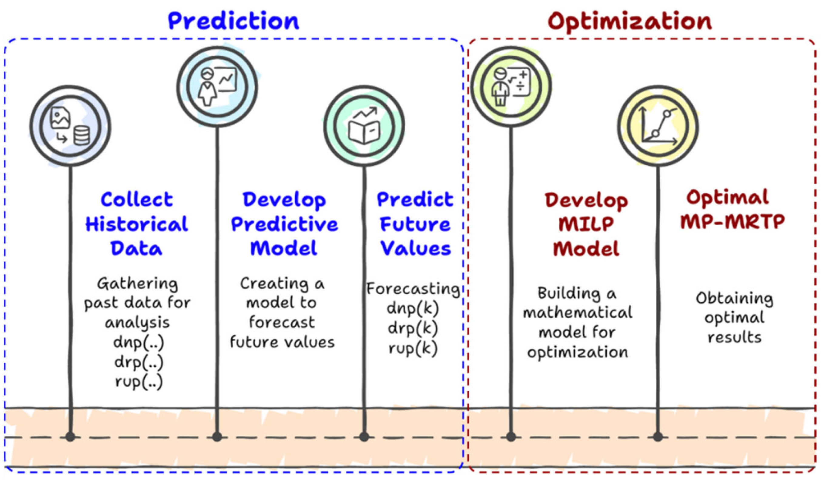
6. Prediction and Optimization Approach

6.1. Two-Stage Framework Approach

To support effective decision-making across multiple planning horizons, the proposed approach integrates prediction and optimization in a two-stage framework as shown in Figure 2 below. In the first stage, key input parameters dnp(k), drp(k), and rup(k) are forecasted over a defined planning horizon (24 periods) using historical data and appropriate predictive methods. These predicted values serve as inputs for the second stage, in which a mixed-integer linear programming (MILP) model is executed to identify the optimal manufacturing, remanufacturing, transportation, and procurement plans.
The two-stage framework outlined above forms the basis of the case study presented in the next section, where we report the predicted values of the key input parameters over the 24-period horizon and demonstrate how these forecasts inform the generation of optimal planning decisions.

6.2. Case Study and Prediction Results

The following section presents the case study and the corresponding prediction results, which serve as the foundation for evaluating the performance and applicability of the proposed optimization approach.

6.2.1. Case Study of an MRTSC

In this section, we illustrate the developed model using a case study of an MRTSC that produces and sells both new and remanufactured microwaves. To support our analysis, we contacted a home appliance sales enterprise and obtained relevant information regarding prices, costs, and demand for microwaves. The collected data provide approximate values for past demand and returned used microwaves shown in Table A1 (see Appendix A), prices of new and remanufactured units, as well as various costs, including inventory and transportation costs shown in Table A2 (see Appendix A). We found that the obtained data are significant and can be used to conduct a study that closely reflects a real MRTSC case. The data that concern carbon emissions and different capacities are empirically chosen. In what follows, the first subsection presents the method for determining the predicted values of dnp(k), drp(k), and rup(k). The second presents the different numerical studies.

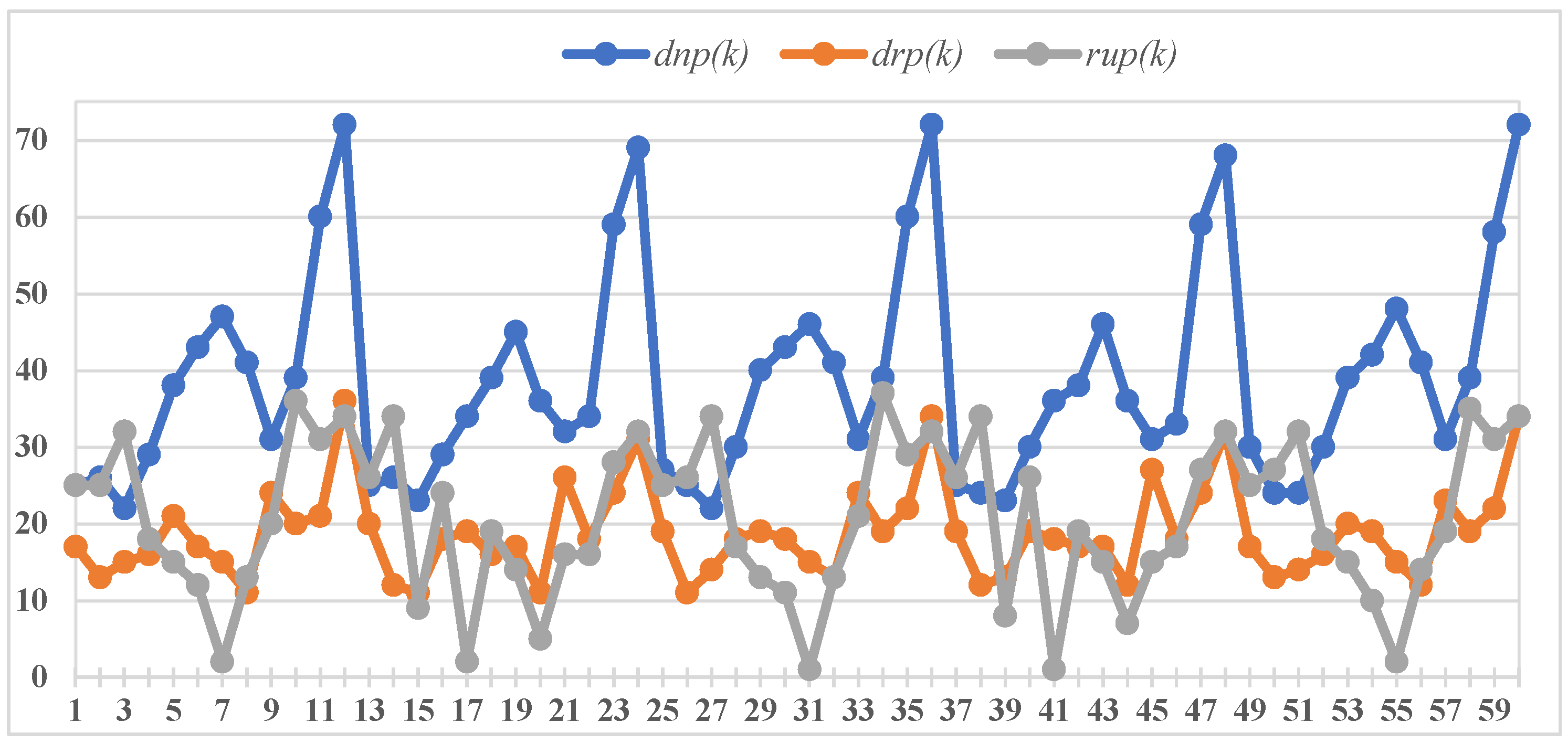
6.2.2. Prediction Results

The following subsection presents the prediction results, starting with the use of machine learning techniques to estimate future values of dnp(k), drp(k), and rup(k). These predicted parameters are essential for guiding the optimization model in the second stage of the proposed framework.

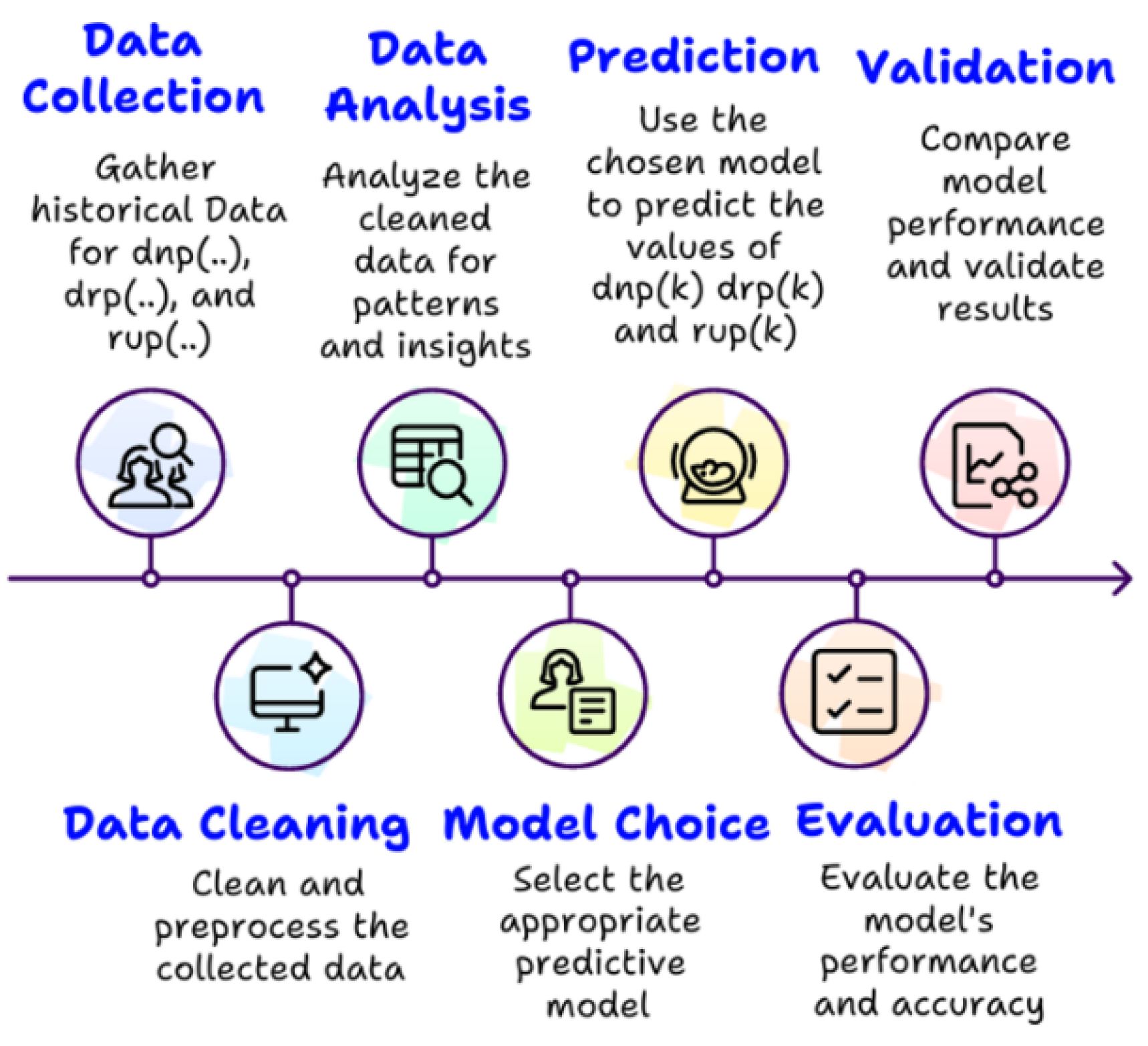
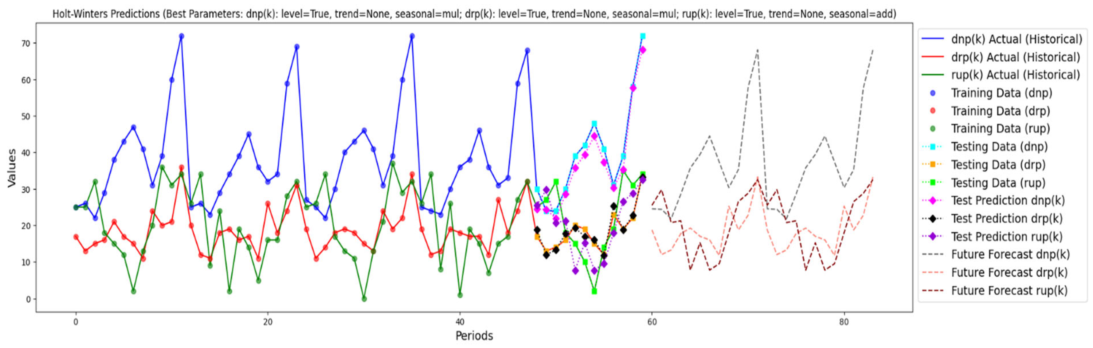
Prediction-Based Machine Learning of Future Values of dnp(k), drp(k), and rup(k)

This subsection targets predicting the future values of dnp(k), drp(k), and rup(k) that will be used as input data for determining the optimal plan over the next 24 periods (planning horizon). The collected data represent the recorded monthly demand values and NRUP over the past 60 periods (i.e., 60 months), which will be used in the different steps of the prediction process shown in Figure 3.

Data Analysis and Selection of Candidate Models

Before analyzing the collected data, we checked whether it was missing any values, contained outliers, or had non-standardized values. We then concluded that the data were clean and ready for use. To analyze the data, we have created a time-series plot for the demands and NRUP over the past 60 periods in Figure 4.
According to the series plot, the demands and NRUP exhibit fluctuations with several peaks and troughs over the observed 60 periods. Furthermore, they do not follow a strict upward or downward trend, meaning they might be influenced by factors. Regarding seasonality, the series of dnp(k) and drp(k) display recurring peaks and troughs every 12 periods. The series of rup(k) also shows repetitive peaks and troughs, but a definitive seasonality cannot be determined. The peaks in the series dnp(k) often coincide with changes in drp(k) and rup(k), indicating a possible interaction and interdependence between the variables. Some movements in the series of rup(k) appear to follow dnp(k) with a delay, indicating a time-lagged relationship. Based on this analysis and our literature study, we suggest five candidate models from the literature that are capable of handling the temporal complexity and interactions: VAR, SARIMA, SARIMA/VAR, LSTM, and HWES.

Prediction and Choice of the Best Model

This section evaluates the candidate models based on their prediction results and metrics. Each model is implemented using a machine learning algorithm that utilizes 80% of the data for training and 20% for testing. It then determines the predicted values (future values) of dnp(k), drp(k), and rup(k). Thus, the candidate algorithms are generated using Python software 3.13.1, and the results are presented below, which include the test evaluation, predicted values, and metrics (RMSE, MAE, R2, and MAPE). We recall that when the values of RMSE and MAE are low (compared to the target variable), R2 > 0.8 and MAPE < 10% indicates good performance of the model. Below, the results are analyzed to identify the best algorithm. Below, each model’s results are presented in a single figure that simultaneously displays the actual collected data, the training data (used to train the model), the testing data (used to evaluate prediction accuracy), the test prediction (results based on the trained model), and the forecasted future values.
  • VAR algorithm
The VAR algorithm differs from the other candidate models by capturing the interdependencies between the three series. It is defined by its key parameter, the maximum lag (referred to as maxlag), which specifies the maximum number of lagged observations included in the model. This parameter determines how many past time steps the algorithm considers when predicting the current values of the system’s variables. Thus, we have elaborated a program that varies the value of “maxlag” and determines the optimal prediction based on the metrics. In our case, the best prediction using the VAR algorithm corresponds to maxlag = 15 with the overall metrics MAE = 1.86, MSE = 6.01, R2 = 0.94, and MAPE = 10.08%.
The results in Figure 5 demonstrate that the VAR algorithm performs acceptable prediction, but the test prediction shows that it lacks precision on the dnp(k) and rup(k) prediction. Although the value of R2 indicates that this algorithm has a good correlation between the prediction and actual data, the values of MAPE and MSE are a little high. This suggests that the model effectively captures the overall trend and relationships between the variables. However, it is highly sensitive to the linearity of these relationships, and when they are nonlinear, the model may fail to make accurate predictions.
  • SARIMA algorithm
The SARIMA differs from the other candidate models by its handles of trend, seasonality, and external effects. Compared to the VAR model, SARIMA is better in capturing seasonality. It performs well with small datasets, where LSTM may struggle. Compared to the HWES model, SARIMA is more flexible for multiplicative seasonality and complex patterns. SARIMA is characterized by its parameters for both non-seasonal (p, d, q) and seasonal (P, D, Q, s) components. Thus, a program is elaborated that varies these parameters and determines the optimal prediction.
The optimal SARIMA parameters, testing, and prediction results are presented in the following figure.
The overall metrics results are MAE = 1.19, MSE = 2.07, R2 = 0.98, and MAPE = 7.76%. The results in Figure 6 demonstrate that the SARIMA algorithm performs excellent prediction. The test prediction shows that predicted curves are expected to closely follow the actual data. The high R2 value and the low MAPE, MAE, and MSE values indicate a strong correlation between the predictions and the actual data for this algorithm.
  • SARIMA/VAR Hybrid algorithm
The SARIMA/VAR model differs from the other candidate models by incorporating trend, seasonality, and multivariate relationships. It is thus characterized by both SARIMA (non-seasonal and seasonal) and VAR (max lag) parameters. A program is integrated into the algorithm to adjust these parameters and identify the optimal prediction. The optimal SARIMA/VAR parameters, testing, and prediction results are presented in Figure 7. Furthermore, the overall metrics results are MAE: 1.19, MSE: 1.99, R2: 0.98, MAPE: 7.61%.
The results in Figure 7 show that the SARIMA/VAR algorithm performs excellent prediction. In addition, the test prediction demonstrates that predicted curves are expected to closely follow the actual data. The high R2 value and the low MAPE, MAE, and MSE values indicate a strong correlation between the predictions and the actual data for this algorithm. Compared to the results of the SARIMA algorithm, the test predictions and future forecasts appear visually similar in Figure 6 and Figure 7. However, when evaluating overall metrics, the SARIMA/VAR model demonstrates slightly better robustness, as it achieves a lower MSE (1.99) and MAPE (7.61%) compared to SARIMA (MSE = 2.07, MAPE = 7.76%).
  • LSTM algorithm
The LSTM differs from other candidate models in that it effectively handles nonlinear relationships and elaborates with both univariate and multivariate data. It is primarily characterized by two parameters: the number of units (neurons) and the depth (number of layers). Therefore, a program is implemented that varies these parameters to determine the optimal prediction. The optimal LSTM parameters, testing, and prediction results are presented in Figure 8. The overall metrics obtained results are MAE: 5.75, MSE: 60.51, R2: 0.68, MAPE: 38.68%.
The results in Figure 8 indicate that the LSTM algorithm delivers poor predictions. Additionally, the test predictions reveal that the predicted curves do not align well with the actual data. The low R2 value, combined with the high MAPE, MAE, and MSE values, suggests a weak correlation between the predictions and the actual data for this algorithm. Despite testing a large number of units, the predictions remain poor, which may be explained by the fact that LSTM requires a large amount of data to generate accurate predictions.
  • HWES algorithm
The HWES captures level, trend, and seasonality using exponential smoothing. These parameters are adjusted automatically in the HWES algorithm for providing optimal prediction. It is known when
-
Level = True\None, means the model includes\not a level component.
-
Trend = True\None, means the model includes\not a trend component.
-
Seasonal = mul\add, means that her seasonality is multiplicative\additive.
The results are given in Figure 9, with the global metrics results as MAE = 2.71, MSE = 13.55, R2 = 0.92, and MAPE = 18.98%.
The test prediction indicates that the algorithm lacks precision and shows a weak correlation between the predicted and actual data. Additionally, although the predictive model achieves decent MAE, MSE, and R2, the high MAPE suggests that it is not very robust, and its inability to adapt to structural changes.
  • Conclusion and choice of the best model
The choice of the model is based on the predictions provided above and also on the metrics results that are summarized in Table 1 below.
Comparing the results in Figure 5, Figure 6, Figure 7, Figure 8 and Figure 9, both the SARIMA and SARIMA/VAR algorithms demonstrate excellent predictive performance and strong correlations between predictions and actual data (Figure 6 and Figure 7). Therefore, the choice of the best model will be between these two. An ideal algorithm should minimize MAE, MSE, and MAPE while maximizing R2. According to the summary table, both models achieve MAE = 1.19 and R2 = 0.98, indicating excellent predictive accuracy. However, SARIMA/VAR outperforms SARIMA by achieving a lower MSE (1.99) and MAPE (7.61%), which signifies higher accuracy and reduced error.
As a result, SARIMA is slightly less accurate than SARIMA/VAR due to its marginally higher MSE and MAPE. Consequently, SARIMA/VAR emerges as the best-performing algorithm, offering superior predictive accuracy with minimal error values. Thus, its prediction results will be used as the future values of dnp(k), drp(k), and rup(k) and they are presented in Table 2 below.

7. Numerical Results

This section aims to simultaneously optimize the quantity ordered for raw materials, manufacturing, remanufacturing, transport, and the returned quantity of used products. Using the solver CPLEX 22.1.1, we experimented by solving the suggested MILP on a laptop equipped with an Intel(R) Core (TM) i3-6006U CPU @2.00 GHz and 3,87 Gb of usable RAM. In fact, we chose to use CPLEX to solve our MILP because it is known as a very robust and reliable solver that includes sophisticated features such as sensitivity analysis. At its core, CPLEX is a set of algorithms used to make decisions. Moreover, it provides good-quality solutions at moderate computational time. The initials values are presented in Table A3 (see Appendix A). Before analyzing the numerical results, the model robustness is discussed in the following subsection.

7.1. The System’s Performance

Based on the numerical results, an optimal profit of 62,421.4 mu is achieved when the unit carbon tax price is equal to 0.01 mu (e.g., ucp = 0.01). This outcome aligns with the optimal plans outlined in Table A4 (see Appendix B). The results observed over the 24-period planning horizon offer valuable insights into the operational behavior of the closed-loop supply chain, particularly regarding production planning, inventory management, and reverse logistics dynamics.
The production schedule of MM (mn(k)) shows a highly variable pattern, with distinct peaks (e.g., k = 3, 17) interspersed with several inactive periods (e.g., k = 4, 7, 12, 14, 16, 18, 20, 23, 24). This non-continuous operation suggests that production is closely guided by demand and raw material availability. Indeed, the quantity of raw materials to order (qrm(k)) appears tightly linked to production demand, with procurement occurring predominantly before or during MM’s active periods.
In parallel, the remanufacturing operations carried out by MR (rm(k)) follow a similarly sporadic pattern but at generally lower volumes, indicating a supportive role in demand satisfaction. The remanufactured products are intended for the S-Market, and their flow appears responsive to the availability of returned items and collection efficiency.
Transportation quantities for both new (trn(k)) and remanufactured (trr(k)) products follow production outputs closely, confirming the efficiency of the outbound logistics system. New product deliveries dominate the flow, aligning with consistent demand in the P-Market. Remanufactured transport is more limited, reflecting either capacity constraints or lower demand in the S-Market.
The transport decision variables (γ1(k) and γ2(k)) indicate an alternating use of two vehicle resources. Initially, vehicle V1 is primarily engaged, with vehicle V2 activated in later periods. This staggered pattern may reflect strategic routing, cost-balancing, or utilization management.
The behavior of warehouse levels further illustrates the system’s responsiveness. The warehouse level of raw materials (wrm(k)) fluctuate significantly, generally increasing during non-production periods and depleting when production resumes. New product inventory (wnp(k)) rises following production peaks, while remanufactured product stock (wrp(k)) remains modest due to limited production.
More concerning are the trends in used product collection (tup(k)) and its subsequent warehousing (wup(k)), which display irregular accumulation patterns. High levels at k = 14, 16, 17 suggest potential delays in remanufacturing or mismatches between returns and processing capacity. The SCP storage (scp(k)) reflects similar build-ups, indicating a need for improved coordination in the reverse logistics flow.
Despite these challenges, customer demand is largely met. The unsatisfied demand quantities (lnp(k) for new, lrp(k) for remanufactured) remain near zero across most periods. Minor shortages in remanufactured products occur at k = 6 and k = 12, coinciding with reduced production and transport to the S-Market.
Sales inventory levels for both product types (inp(k) and irp(k)) show gradual accumulation, suggesting a strategy of buffering against future demand surges. However, care must be taken to avoid excessive holding costs or product obsolescence, particularly in the case of remanufactured goods.
Finally, sales data (vnp(k) and vrp(k)) confirm that new products consistently outsell remanufactured ones, especially in the middle of the planning horizon. This aligns with production priorities and possibly reflects stronger consumer preference for new products in the P-Market, though the S-Market shows a steady if limited uptake.
In summary, the proposed system demonstrates a high degree of adaptability across both forward and reverse logistics operations. It consistently maintains strong service levels through flexible production planning and responsive transport scheduling. While certain inefficiencies remain particularly within the reuse and remanufacturing processes, these highlight actionable areas for further optimization. In particular, improving the alignment between return collection rates, remanufacturing capacity, and secondary market demand presents a valuable opportunity for enhancing overall system performance. Moreover, the results presented clearly illustrate the robustness of the model under varying operational conditions. Despite fluctuations in demand and production, as well as the inherent complexities of managing reverse flows, the system sustained stable service levels and minimized unsatisfied demand throughout the planning horizon. This reliable performance not only affirms the model’s effectiveness as a decision-support tool but also reinforces its value as a practical performance indicator for evaluating the efficiency and responsiveness of a closed-loop supply chain.
Building upon this analysis, the following sub-section examines the system’s performance under environmentally driven constraints, specifically the impact of carbon tax pricing on total carbon footprint and profit.

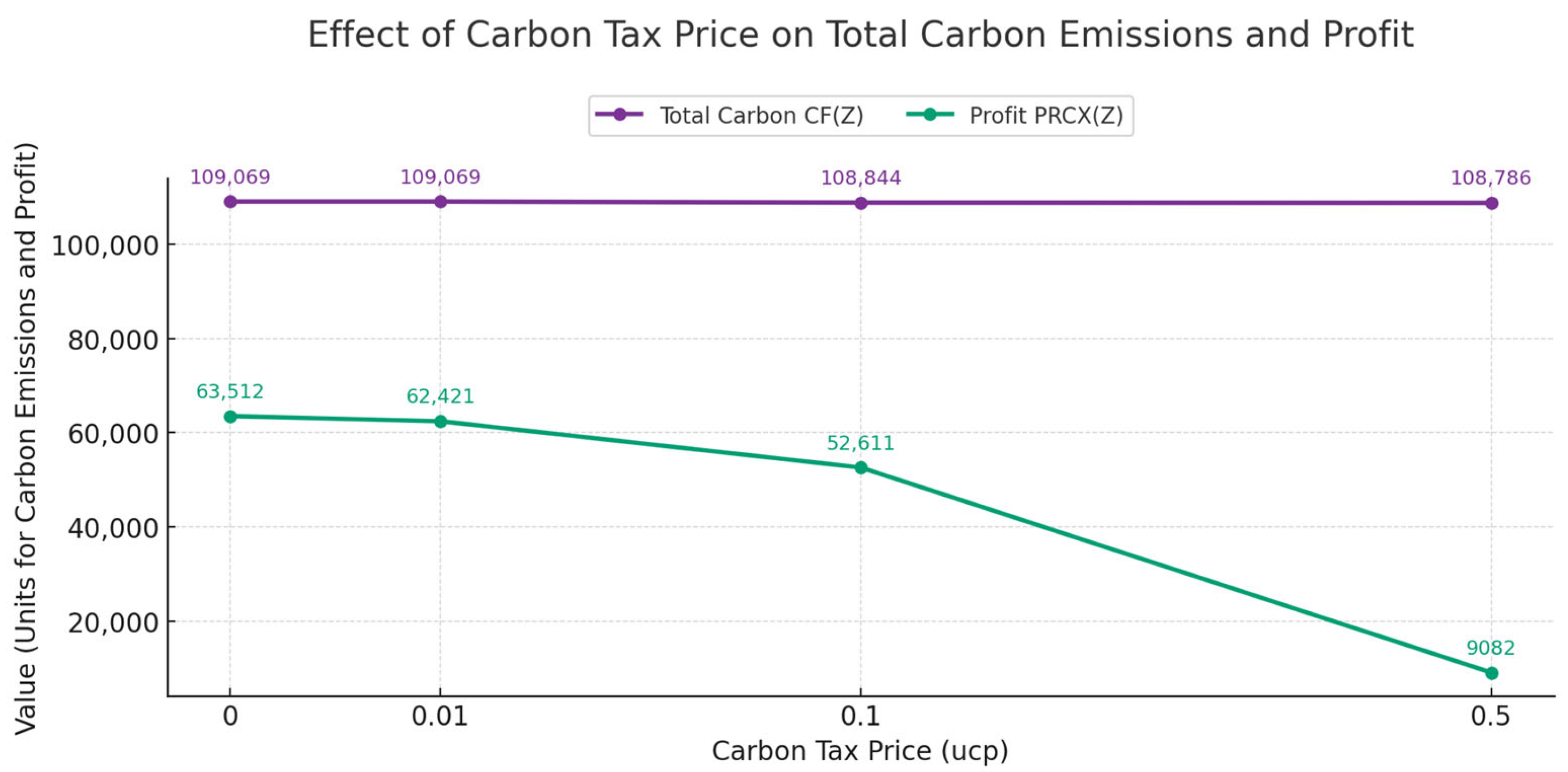
7.2. Results Based on Carbon Tax Price

Based on the numerical results, an optimal profit of 63,512 mu is achieved when no financial penalty is imposed on carbon emissions. This outcome aligns with the optimal plans outlined in Table A5 (see Appendix B). The results clearly indicate that both manufacturing and remanufacturing activities adjust in response to demand fluctuations to ensure a steady supply of selling inventories. Similarly, transportation plans evolve accordingly, adapting to variations in demand to maintain efficient inventory distribution across selling stores. Moreover, the order plan for raw materials is directly influenced by manufacturing requirements. When an adequate supply of raw materials is available for production, additional orders are unnecessary, resulting in an order quantity of zero during such periods. This relationship between production planning and financial considerations becomes even more evident when analyzing the effects of carbon taxation, as shown in Figure 10, where the interplay between emission regulations and economic performance is further explored. The results shown illustrate the impact of carbon tax pricing on total carbon emissions and profit within the system. As observed, the total carbon footprint (CF(Z) remains relatively stable, with only a slight decrease as the carbon tax price (ucp) increases. This suggests that within the studied range, the imposed tax is not substantial enough to drive significant emission reductions. However, the profit PRCX(Z) shows a sharp decline, particularly beyond ucp = 0.01, indicating that the financial burden of the carbon tax directly affects economic performance. At ucp = 0.5, profit drops drastically, highlighting a strong trade-off between sustainability policies and economic viability. These findings suggest that while carbon taxation serves as a regulatory tool, its effectiveness in reducing emissions may be limited unless coupled with incentives for cleaner technologies or more stringent tax rates. Moreover, businesses may need to adopt alternative sustainability strategies to mitigate financial losses while complying with environmental policies.
The implications of carbon taxation extend beyond individual economic systems and align with global initiatives aimed at mitigating climate change. This is exemplified by the Paris Agreement, which establishes a structured framework for reducing carbon emissions through international cooperation, policy implementation, and sustainable economic strategies.

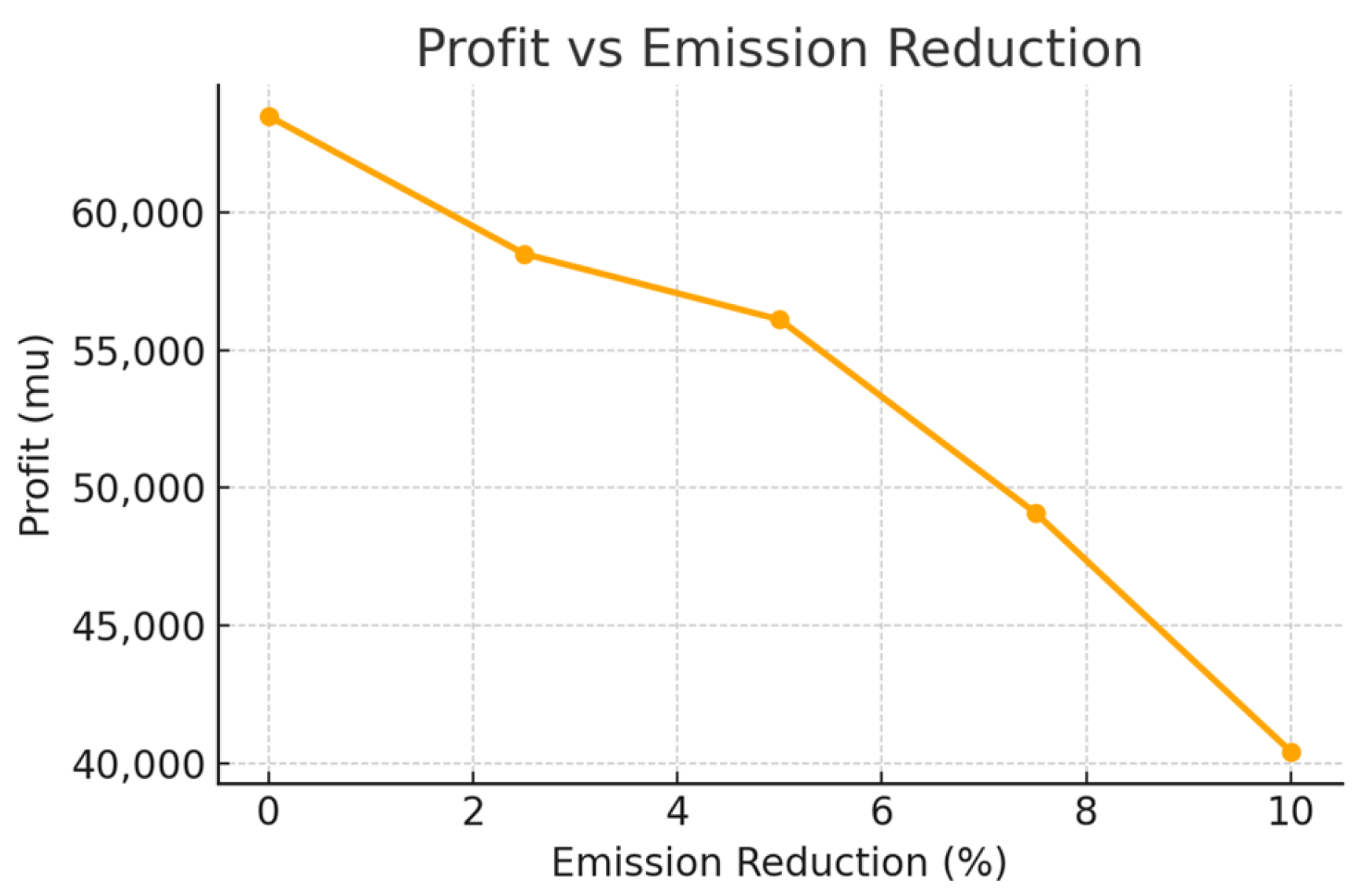
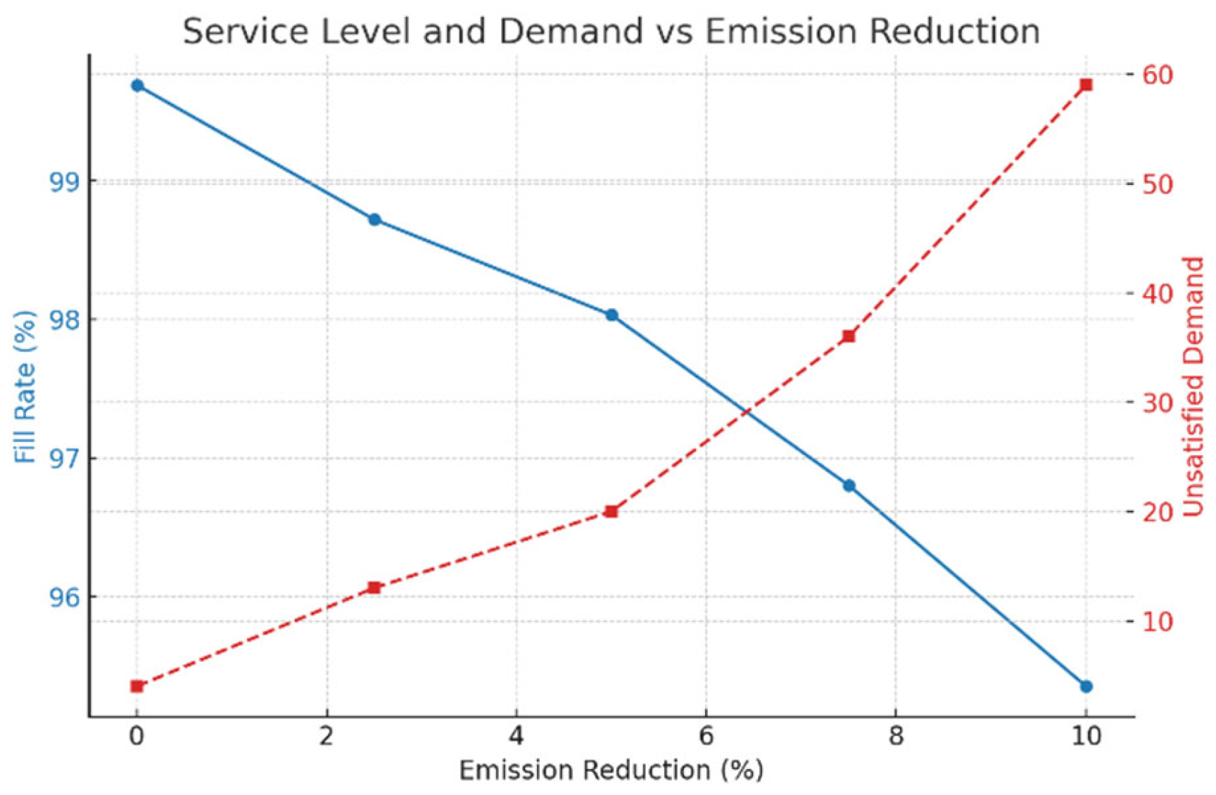
7.3. Based on Paris Agreement Limitation

The Paris Agreement represents a landmark global strategy aimed at reducing carbon emissions and mitigating climate change impacts. Adopted in 2015 during COP21, the agreement aims to limit the rise in global temperature to significantly below 2 °C, with efforts to cap warming at 1.5 °C above pre-industrial levels. It establishes a framework where participating nations submit and regularly update their Nationally Determined Contributions (NDCs), outlining targeted reductions in greenhouse gas (GHG) emissions [31]. A key aspect of the agreement is the promotion of carbon pricing mechanisms, renewable energy expansion, and sustainable industrial practices to achieve long-term decarbonization. Furthermore, developed nations commit to providing financial and technological support to assist developing countries in adopting low-carbon solutions and enhancing climate resilience. Despite its voluntary nature, the Paris Agreement serves as a critical driver of carbon emission reduction, encouraging global cooperation, innovation, and policy development to transition toward a net-zero future.
The results presented in Table 3 illustrate the trade-off between carbon emission reduction, economic performance, and service levels in the studied system. Under unrestricted emissions, the highest profit of 63,512.1 mu is achieved, with a total carbon footprint of 109,069 and a 99.69% order fill rate, indicating near-optimal operational efficiency. However, as emission reduction constraints are introduced, a progressive decline in profit is observed, reflecting the increasing financial burden associated with emission limitations.
For instance, at a 2.5% reduction, profit decreases to 58,510.1 mu, with a loss of earnings of 5002 mu, while total carbon emissions drop to 106,336 carbon units. Further reductions to 5%, 7.5%, and 10% resulted in even greater losses, with profits declining to 56,118, 49,098.3, and 40,413.2, respectively. At the 10% emissions reduction level, profit declines sharply, accompanied by the highest loss of earnings at 23,098.9, demonstrating the significant financial impact of stringent carbon constraints.
The order fill rate also deteriorates as carbon reduction targets increase, dropping from 99.69% without limitation to 95.35% at a 10% reduction. This decline correlates with an increase in unsatisfied demand, particularly for new products (lnp(k)), which rose from 0 to 35 units to the highest reduction level. Similarly, the total of unsatisfied demand (lnp(k) + lrp(k)) increases from 4 to 59, suggesting that stricter emission policies may lead to supply shortages, affecting service reliability.
These findings highlight the delicate balance between sustainability efforts and economic viability. While carbon emission reductions contribute to environmental sustainability, they impose financial costs and operational challenges, particularly in maintaining profitability and service levels. Therefore, effective carbon reduction strategies should integrate cost-efficient technological innovations and policy incentives to minimize adverse economic impacts while promoting sustainability goals.
To better illustrate the findings in Table 3 related to the impact of carbon reduction policies on operations and profitability, we have included two charts based on the decision matrix. The first chart shown in Figure 11 below displays how profit steadily declines as emission reduction targets increase. With a 0% reduction, the system achieves its highest profitability. However, as the constraints tighten, moving toward the 10% cut, profits drop significantly. This clearly reflects the financial pressure that can come with stricter environmental targets. The second chart shown in Figure 12 helps visualize how service performance is affected. As the fill rate decreases, the amount of unsatisfied demand rises sharply. This means that beyond a certain threshold, aggressive carbon cuts may begin to interfere with the company’s ability to meet customer needs reliably.
Together, these charts provide a clearer picture for decision-makers showing not just the environmental benefit of reducing emissions, but also the cost and trade-offs that come with it. They can help managers strike the right balance between sustainability goals and business performance.
From a managerial perspective, the findings underline the importance of aligning environmental responsibility with operational resilience. The gradual decline in profit and service levels as carbon constraints tighten suggests that emission reduction targets, if not paired with adaptive strategies, may strain supply chains and limit growth. Managers must anticipate these trade-offs by investing in cleaner production methods, diversifying supply sources, and optimizing resource usage to maintain service reliability under stricter regulations. In light of the Paris Agreement’s ambitions, businesses operating under such frameworks will need to integrate carbon performance into their core decision-making treating emissions not just as an environmental issue but as a financial and strategic variable. Proactive planning, scenario testing, and collaboration with policymakers can help firms stay competitive while supporting long-term climate goals.

7.4. Theoretical and Managerial Implications of the Model

The proposed model enhances the theoretical foundations of sustainable supply chain management by presenting a unified framework that explicitly integrates multi-period planning with carbon emissions constraints and demand uncertainty. By embedding predictive forecasting methods directly within the optimization structure, this work advances theoretical understanding of how anticipatory decision-making can be effectively operationalized under environmental regulations. Unlike traditional models that treat demand and emissions as exogenous or static, our approach illustrates how dynamic, data-driven inputs can shape production, transportation, and inventory strategies over time. Furthermore, the integration of hybrid forecasting techniques such as SARIMA/VAR expands existing theory on closed-loop systems, demonstrating how multivariate temporal relationships can be utilized to improve planning accuracy. These contributions lay the groundwork for future models aiming to align environmental policy compliance with operational efficiency in complex, real-world supply chains.
From a managerial standpoint, the proposed model serves as a practical decision-making tool for supply chain managers operating in an increasingly complex and regulated landscape. By integrating production, remanufacturing, and transportation decisions across multiple planning periods, it enables managers to align operational efficiency with environmental sustainability. The incorporation of forecasting techniques adds further value, empowering managers to proactively anticipate demand trends and allocate resources effectively, rather than merely reacting to changes. A key advantage of the model is its capacity to simulate carbon trade-offs, providing managers with clearer insights into how regulatory policies, such as carbon pricing or emissions caps, could impact their operations. This facilitates more informed, long-term planning, particularly in scenarios involving uncertainty or sustainability targets. Ultimately, the model fosters a strategic, forward-thinking approach to sustainable supply chain management.

8. Conclusions

This study developed and analyzed a comprehensive optimization model for multi-period planning in a closed-loop supply chain, with particular attention to manufacturing, remanufacturing, and transport activities under carbon-related constraints. By integrating forward and reverse flows, the model captures the operational complexities of a system designed to meet demand while respecting environmental limitations, such as carbon taxes and emissions targets.
Through detailed scenario analyses, the model demonstrated a strong capacity to adapt to variable production schedules, fluctuating return flows, and shifting demand, all while maintaining service levels and minimizing both inventory excesses and unmet demand. Its performance under both economic and environmental constraints highlights its potential as a practical decision-support tool for supply chain managers aiming to balance profitability with regulatory compliance and sustainability objectives.
An important contribution of this work involves the integration of demand forecasting methods directly into the optimization framework. Advanced predictive models such as Vector Autoregression (VAR), Seasonal ARIMA (SARIMA), hybrid SARIMA/VAR, Long Short-Term Memory (LSTM) networks, and Holt–Winters Exponential Smoothing (HWES) offer promising avenues for improving forecast accuracy. Among the forecasting methods evaluated, the hybrid SARIMA/VAR model proved to be the most effective, offering the highest level of predictive accuracy with consistently minimal error values. Its ability to capture both seasonal patterns and cross-variable relationships makes it particularly well-suited for anticipating demand and return dynamics in a closed-loop supply chain context. Given its performance, the predictions generated by the SARIMA/VAR model will be adopted as the basis for estimating future values of key input parameters, namely dnp(k), drp(k), and rup(k). Incorporating these forecasted values into the optimization framework strengthens the model’s ability to respond to uncertainty and enhances its utility as a proactive planning tool under environmental and operational constraints.
Moreover, the inclusion of carbon pricing mechanisms and Paris Agreement-aligned limitations offers valuable insight into the trade-offs between operational efficiency and environmental impact. The model thus contributes meaningfully to the growing body of research at the intersection of supply chain optimization and climate policy. Future extensions may include uncertainty modeling, real-time decision updates, or broader network configurations to further explore the model’s applicability in more complex or decentralized settings. On the forecasting side, while the hybrid SARIMA/VAR model delivered strong results, there is clear potential to experiment with ensemble-based approaches that combine statistical and machine learning methods. From a regulatory and policy perspective, future work could consider uncertainty in carbon markets by incorporating fluctuating carbon prices, cap-and-trade mechanisms, or differentiated tax regimes.

Author Contributions

Methodology, B.A. and S.T.; Software, S.T.; Validation, B.A. and S.D.; Formal analysis, B.A.; Investigation, S.D. and B.A.; Writing—original draft, B.A.; Supervision S.D. and S.T. All authors have read and agreed to the published version of the manuscript.

Funding

This research received no external funding.

Institutional Review Board Statement

Not applicable.

Informed Consent Statement

Not applicable.

Data Availability Statement

Due to the commercially sensitive nature of this research, supporting data is not available.

Conflicts of Interest

The authors declare no conflict of interest.

Appendix A. Additional Data and Tables

Table A1. Collected data during 60 periods.
Perioddnp(k)drp(k)rup(k)Perioddnp(k)drp(k)rup(k)Perioddnp(k)drp(k)rup(k)
1251725213226164136181
22613252234181642381719
32215322359242843461715
4291618246931324436127
53821152527192545312715
64317122625112646331817
7471522722143447592427
84111132830181748683232
93124202940191349301725
103920363043181150241327
11602131314615151241432
127236343241131352301618
132520263331242153392015
142612343439193754421910
1523119356022295548152
162918243672343256411214
17341923725192657312319
183916193824123458391935
19451714392313859582231
20361154030192660723434
Table A2. Model parameters and their values.
Parameter SymbolValueParameter SymbolValue
Z24NP220
Z. λ24RP200
x18N160
a75R110
b20SP150
wx0.1TRV170
wa0.5TRV2100
wb0.4GM80
ct1GR60
ca3.5em5 carbon units
cb3en60 carbon units
cs1er10 carbon units
y15erm1 carbon units
sn400ewn2 carbon units
sr320ewr2 carbon units
FT1500esc1 carbon units
FT2600ecu1 carbon units
pn145enp3 carbon units
pr110erp3 carbon units
pv17etr1 carbon units
ucp0.01efrt12500 carbon units
RM150efrt22800 carbon units
Table A3. Initial values of model parameters.
Parameter SymbolValueParameter SymbolValue
dnp050wup010
drp040scp010
rup010inp030
qrm030irp020
mn030vnp050
rm020vrp040
trn030lnp00
trr020lrp00
tup010γ1(k)1
wrm030γ2(k)0
wnp020vup00
wrp030CF00

Appendix B. Additional Results

Table A4. Optimal plans with ucp = 0.01.
k123456789101112131415161718192021222324
mn(k)162674043640356468380450660740570566500
rm(k)0152601533034632320250340260430233100
qrm(k)5604364035646838045066074057056650000
trn(k)1719267404364035646838045066074057056650
trr(k)81324260153303463232025034026043023310
tup(k)23253216023003235293205703201701902900
wnp(k)192674043640356468380450660740570566500
wrp(k)22242601533034632320250340260430233100
wrm(k)44740436403564683804506607405705665000
wup(k)33434965504040632353264399662946885426138363636
scp(k)232532161323013323529322557832017141914292757
vnp(k)262119263539433628355569242220253135413327305665
vrp(k)171113161915151122192132181011181716171025182331
inp(k)21192674394364283564774622452566357433573056650
irp(k)11132434151533223421323214291834172710431823310
lnp(k)000000000000000000000000
lrp(k)000002000002000000000000
vup(k)000000000000000000000000
γ1(k)111001001101010000000000
γ2(k)000100100010000101010110
Table A5. Optimal plans with ucp = 0.
k123456789101112131415161718192021222324
mn(k)162674043640356468380450660740570566500
rm(k)0152601533034632320250340260430233100
qrm(k)5604364035646838045066074057056650000
trn(k)1719267404364035646838045066074057056650
trr(k)81324260153303463232025034026043023310
tup(k)23253216023003235293205703201701902900

References

  1. Karim, R.; Roshid, M.M.; Waaje, A. Circular Economy and Supply Chain Sustainability. In Strategic Innovations for Dynamic Supply Chains; IGI Global: Hershey, PA, USA, 2024; pp. 1–30. [Google Scholar]
  2. Hajipour, V.; Kaveh, S.H.; Yiğit, F.; Gharaei, A. A multi-objective supply chain optimization model for reliable remanufacturing problems with M/M/m/k queues. Supply Chain. Anal. 2025, 10, 100118. [Google Scholar] [CrossRef]
  3. Cheng, F.; Jia, S.; Gao, W. Low-Carbon Logistics Distribution Vehicle Routing Optimization Based on INNC-GA. Appl. Sci. 2024, 14, 3061. [Google Scholar] [CrossRef]
  4. Salas-Navarro, K.; Castro-García, L.; Assan-Barrios, K.; Vergara-Bujato, K.; Zamora-Musa, R. Reverse Logistics and Sustainability: A Bibliometric Analysis. Sustainability 2024, 16, 5279. [Google Scholar] [CrossRef]
  5. Alkahtani, M.; Ziout, A.; Salah, B.; Alatefi, M.; Abd Elgawad, A.E.E.; Badwelan, A.; Syarif, U. An Insight into Reverse Logistics with a Focus on Collection Systems. Sustainability 2021, 13, 548. [Google Scholar] [CrossRef]
  6. Zhang, X.; Zou, B.; Feng, Z.; Wang, Y.; Yan, W. A Review on Remanufacturing Reverse Logistics Network Design and Model Optimization. Processes 2021, 10, 84. [Google Scholar] [CrossRef]
  7. Dam, S.; Bakker, C. Between a Rock and a Hard Place. A Case Study on Simplifying the Reverse Logistics of Car Parts to Enable Remanufacturing. J. Circ. Econ. 2024, 2, 1–23. [Google Scholar]
  8. Mbago, M.; Ntayi, J.M.; Mkansi, M.; Namagembe, S.; Tukamuhabwa, B.R.; Mwelu, N. Implementing reverse logistics practices in the supply chain: A case study analysis of recycling firms. Mod. Supply Chain Res. Appl. 2025. ahead of print. [Google Scholar] [CrossRef]
  9. Muchenje, K. Green Logistics and Supply Chain Management. In Contemporary Solutions for Sustainable Transportation Practices; IGI Global: Hershey, PA, USA, 2024; pp. 33–61. [Google Scholar]
  10. Yin, C.; Zhang, Z.A.; Fu, X.; Ge, Y.E. A low-carbon transportation network: Collaborative effects of a rail freight subsidy and carbon trading mechanism. Transp. Res. Part A Policy Pract. 2024, 184, 104066. [Google Scholar] [CrossRef]
  11. Sifaoui, T.; Aïder, M. Beyond green borders: An innovative model for sustainable transportation in supply chains. RAIRO Oper. Res. 2024, 58, 2185–2237. [Google Scholar] [CrossRef]
  12. Abassi, B.; Turki, S.; Dellagi, S.; Bellamine, I. Low-carbon manufacturing-remanufacturing supply chain: Systematic review and bibliometric analysis. Supply Chain Forum Int. J. 2025, 204, 160–173. [Google Scholar] [CrossRef]
  13. Metcalf, G.E.; Stock, J.H. The Macroeconomic Impact of Europe’s Carbon Taxes. Am. Econ. J. Macroecon. 2023, 15, 265–286. [Google Scholar] [CrossRef]
  14. Stechemesser, A.; Koch, N.; Mark, E.; Dilger, E.; Klösel, P.; Menicacci, L.; Nachtigall, D.; Pretis, F.; Ritter, N.; Schwarz, M.; et al. Climate policies that achieved major emission reductions: Global evidence from two decades. Science 2024, 385, 884–892. [Google Scholar] [CrossRef] [PubMed]
  15. Yang, W.; Li, H.; Shi, J. Collaborative innovation in low-carbon supply chain under cap-and-trade: Dual perspective of contracts and regulations. J. Clean. Prod. 2025, 499, 145223. [Google Scholar] [CrossRef]
  16. Ding, J. Design of a low carbon economy model by carbon cycle optimization in supply chain. Front. Ecol. Evol. 2023, 11, 1122682. [Google Scholar] [CrossRef]
  17. Wang, J.; Wang, D.; Yuan, Y. Research on low-carbon closed-loop supply chain strategy based on differential games-dynamic optimization analysis of new and remanufactured products. AIMS Math. 2024, 9, 32076–32101. [Google Scholar] [CrossRef]
  18. Mirzaee, H.; Samarghandi, H.; Willoughby, K. A robust optimization model for green supplier selection and order allocation in a closed-loop supply chain considering cap-and-trade mechanism. Expert Syst. Appl. 2022, 228, 120423. [Google Scholar] [CrossRef]
  19. Turki, S.; Jemmali, M.; Hidri, L. Optimal control for unreliable manufacturing and remanufacturing system under environmental subsidy and overrun penalty mechanism. IEEE Trans. Eng. Manag. 2025, 72, 1983–2002. [Google Scholar] [CrossRef]
  20. Mecheter, A.; Pokharel, S.; Tarlochan, F.; Tsumori, F. A multi-period multiple parts mixed integer linear programming model for AM adoption in the spare parts supply Chain. Int. J. Comput. Integr. Manuf. 2024, 37, 550–571. [Google Scholar] [CrossRef]
  21. Hamzaoui, A.F.; Malek, M.; Zied, H.; Sadok, T. Optimal production and non-periodic maintenance plan for a degrading serial production system with uncertain demand. Int. J. Syst. Sci. Oper. Logist. 2023, 10, 2235808. [Google Scholar] [CrossRef]
  22. Wang, J.; Rickman, D.; Yu, Y. Dynamics between global value chain participation, CO2 emissions, and economic growth: Evidence from a panel vector autoregression model. Energy Econ. 2022, 109, 105965. [Google Scholar] [CrossRef]
  23. Brucke, K.; Schmitz, S.; Köglmayr, D.; Baur, S.; Räth, C.; Ansari, E.; Klement, P. Benchmarking reservoir computing for residential energy demand forecasting. Energy Build. 2024, 314, 114236. [Google Scholar] [CrossRef]
  24. Wolny, M.; Kmiecik, M. Unveiling Patterns in Forecasting Errors: A Case Study of 3PL Logistics in Pharmaceutical and Appliance Sectors. Sustainability 2025, 17, 214. [Google Scholar] [CrossRef]
  25. Zhao, Y. E-Commerce Demand Forecasting Using SARIMA Model and K-means Clustering Analysis. J. Innov. Dev. 2024, 7, 1–6. [Google Scholar] [CrossRef]
  26. Falatouri, T.; Darbanian, F.; Brandtner, P.; Udokwu, C. Predictive Analytics for Demand Forecasting—A Comparison of SARIMA and LSTM in Retail SCM. Procedia Comput. Sci. 2022, 200, 993–1003. [Google Scholar] [CrossRef]
  27. Koohikeradeh, E.; Gumiere, S.; Bonakdari, H. NDMI-Derived Field-Scale Soil Moisture Prediction Using ERA5 and LSTM for Precision Agriculture. Sustainability 2025, 17, 2399. [Google Scholar] [CrossRef]
  28. Fuqua, D.; Hespeler, S. Commodity demand forecasting using modulated rank reduction for humanitarian logistics planning. Expert Syst. Appl. 2022, 206, 117753. [Google Scholar] [CrossRef]
  29. Ahlaqqach, M.; Elkourchi, A.; Ali Moulay, E.O. Demand Forecast of Pharmaceutical Products During COVID-19 Using Holt-Winters Exponential Smoothing. In International Conference on Artificial Intelligence & Industrial Applications; Springer Nature: Cham, Switerland, 2023; Volume 772, pp. 427–437. [Google Scholar]
  30. Tsigler, A.; Bartlett, P.L. Benign overfitting in ridge regression. J. Mach. Learn. Res. 2023, 24, 1–76. [Google Scholar]
  31. Chiquier, S.; Fajardy, M.; Dowell, N. CO2 removal and 1.5 °C: What, where, when, and how? Energy Adv. 2022, 1, 524–561. [Google Scholar] [CrossRef]
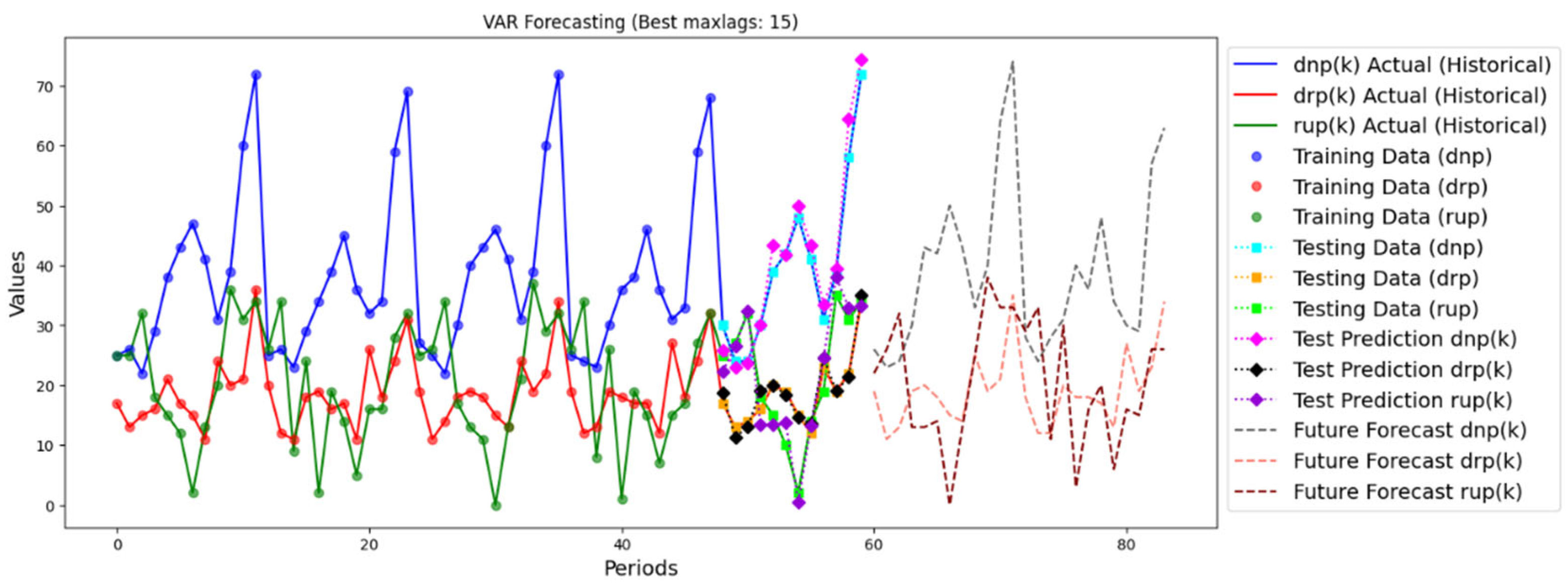
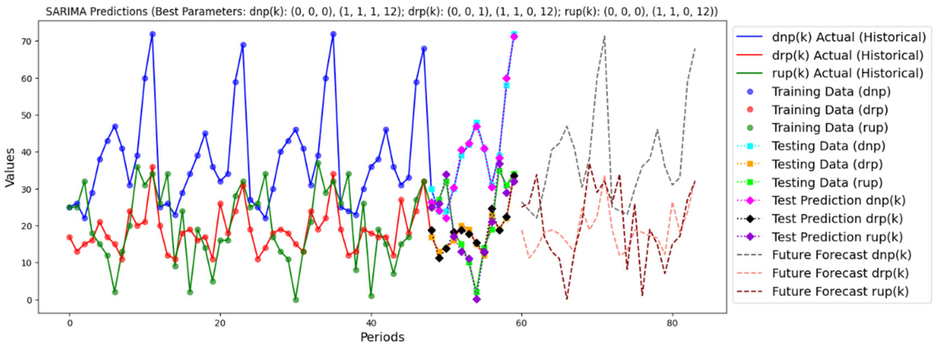
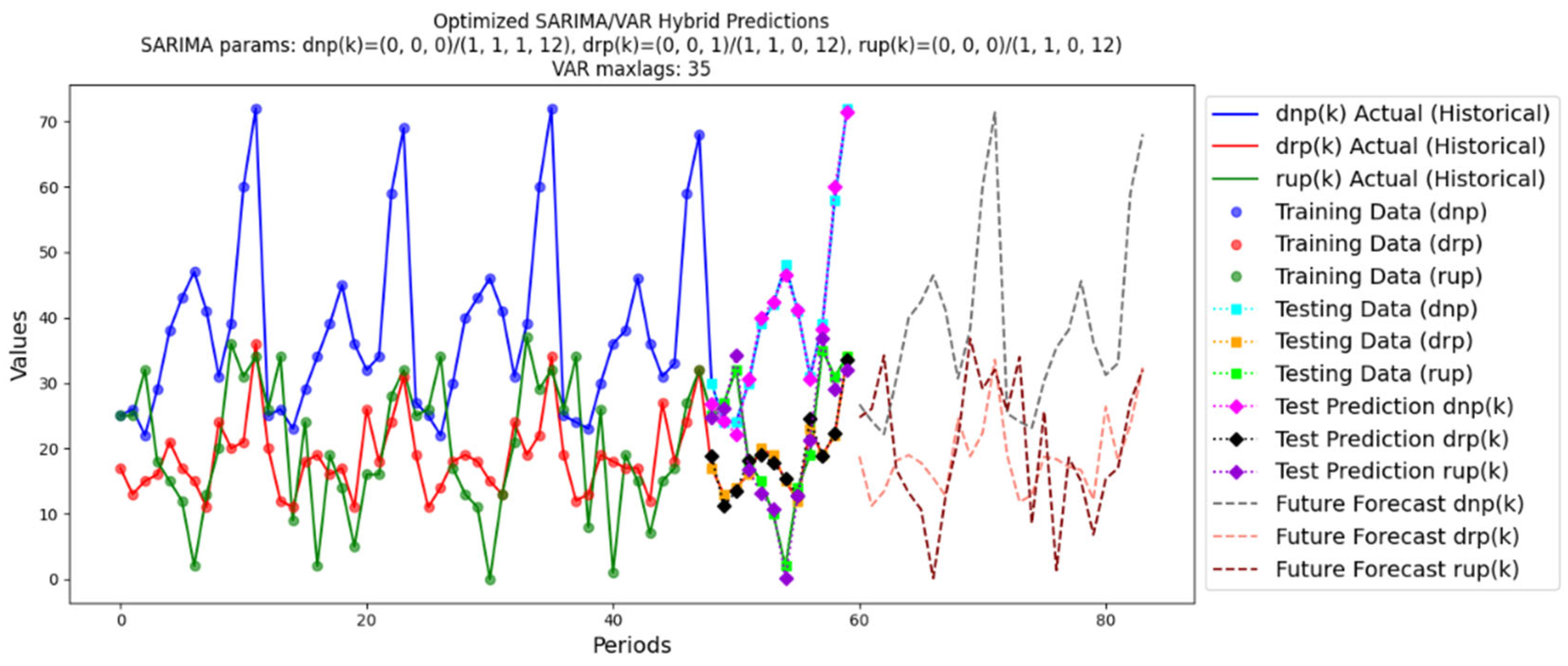
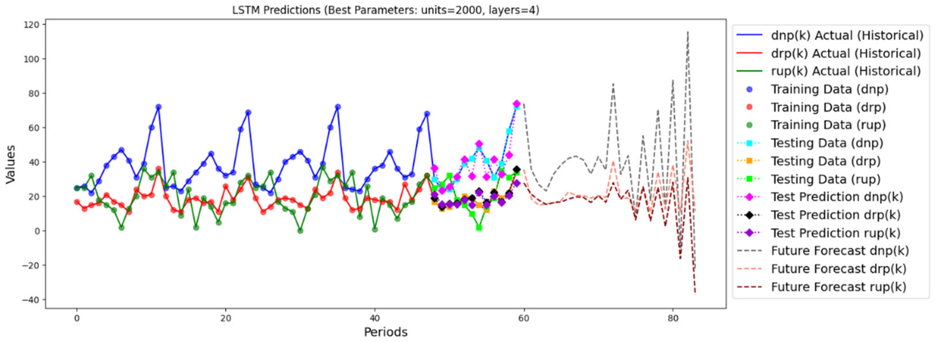
Figure 1. Comprehensive Sustainable Supply Chain.
Sustainability 17 05218 g001
Figure 2. Comprehensive approach.
Sustainability 17 05218 g002
Figure 3. Prediction process.
Sustainability 17 05218 g003
Figure 4. Time-series plot for dnp(k), drp(k), and rup(k).
Sustainability 17 05218 g004
Figure 5. VAR prediction.
Sustainability 17 05218 g005
Figure 6. SARIMA prediction.
Sustainability 17 05218 g006
Figure 7. SARIMA/VAR prediction.
Sustainability 17 05218 g007
Figure 8. LSTM prediction.
Sustainability 17 05218 g008
Figure 9. HWES prediction.
Sustainability 17 05218 g009
Figure 10. Impact of carbon tax pricing on total carbon footprint and profit.
Sustainability 17 05218 g010
Figure 11. Impact of emission reduction targets on profitability.
Sustainability 17 05218 g011
Figure 12. Effect of carbon constraints on service level and demand fulfillment.
Sustainability 17 05218 g012
Table 1. Comparison of metrics results.
AlgorithmMAE aMSE bR2 cMAPE d
VAR1.866.010.9410.08%
SARIMA1.192.070.987.76%
SARIMA/VAR1.191.990.987.61%
LSTM5.7560.510.6838.68%
HWES2.7113.550.9218.98%
a MAE: Mean Absolute Error; b MSE: Mean Squared Error; c R2: Coefficient of Determination; d MAPE: Mean Absolute Percentage Error; SARIMA/VAR achieved the best overall performance with the lowest MSE and MAPE.; LSTM performed significantly worse in this dataset, with the highest error values across all metrics.
Table 2. Predicted customer demands and returned used products of two future years (Z = 24, period k = 1, …, Z).
k123456789101112131415161718192021222324
dnp(k) a262119263539433628355569242220253135413327305665
drp(k) b171113161917151122192134181011181716171025182331
rup(k) c23253216131001319352932253282401714514152730
a dnp(k): Predicted demand for new products in period kb drp(k): Predicted demand for refurbished products in period kc rup(k): Predicted quantity of returned used products in period k; Highest new product demand occurs at k = 12 (69 units), suggesting a peak period in the first year. The lowest return quantity is observed at k = 7 and 17, indicating no used product inflow. A significant increase in both demand and returns is noticeable in the second half of the planning.
Table 3. Trade-off between carbon emission reduction, economic performance, and service levels.
CaseProfit
PRCX(Z)
Total Carbon CF(Z)Loss of EarningsTotal of lnp(k) aTotal of lrp(k) bTotal of lnp(k) and lrp(k)Global Service Level (Order Fill Rate)
Without limitation63,512.1109,069004499.69%
2.5% reduction compared to emissions without limitation58,510.1106,33650021241698.74%
5% reduction compared to emissions without limitation56,118103,6157394.11742198.35%
7.5% reduction compared to emissions without limitation49,098.3100,88814,413.82983797.09%
10% reduction compared to emission without limitation40,413.298,16223,098.935245995.35%
a lnp(k): unmet demand for new products; b lrp(k): unmet demand for regular products. A significant profit drop begins beyond 5% emission cut; total unmet demand surpasses 50 units at 10% reduction, indicating potential bottlenecks; order fill rate falls below 96% under 10% cut, highlighting service performance risk.
Disclaimer/Publisher’s Note: The statements, opinions and data contained in all publications are solely those of the individual author(s) and contributor(s) and not of MDPI and/or the editor(s). MDPI and/or the editor(s) disclaim responsibility for any injury to people or property resulting from any ideas, methods, instructions or products referred to in the content.

