Evaluating the Health Risks of Air Quality and Human Thermal Comfort–Discomfort in Relation to Hospital Admissions in the Greater Athens Area, Greece

Abstract

The aim of this study is to examine the impact of poor air quality and adverse meteorological conditions on health risks in the Greater Athens Area (GAA), Greece, during the period from 2018 to 2022. Specifically, the aim is to assess the Relative Risk (RR) of hospital admissions (HAs) for cardiovascular diseases (CVDs) and respiratory diseases (RDs), due to air pollution in combination with thermal discomfort, as well as to identify the time lag effect on admissions. For this purpose, data from six (6) different hospitals within the GAA were collected and used. Statistical analysis of hourly measurements of key pollutants (NO₂, O₃, PM_2.5, and PM₁₀) obtained from the Directorate of Climate Change and Air Quality (DCCAQ), which falls under the auspices of the Ministry of Environment and Energy (MEE), and meteorological parameters (T, RH, and wind velocity), is performed to calculate the daily air quality and human thermal comfort–discomfort levels, respectively. These conditions were examined using appropriate indexes for both air quality and human thermal comfort–discomfort, as independent variables in a Negative Binomial regression model developed in R, with daily HAs (not including scheduled cases or pre-existing health conditions) as the response variable. Moreover, a spatiotemporal analysis of air quality and meteorological parameters is conducted to identify associated variations in health risks. This analysis highlights key risk patterns linked to environmental conditions and the relevant measures to both manage and mitigate the risk. Findings indicate that extreme environmental conditions significantly elevate health risks, with cumulative RR over a one-week period peaking at 1.540 (95% CI: 1.158–2.050) during the warm season, while prolonged increases in the RR are also observed during the cold season, reaching 1.214 (95% CI: 0.937–1.572) under extreme cold exposures.

1. Introduction

Air pollution represents a significant environmental issue with profound implications for human health, particularly in urban areas where anthropogenic pollutant emissions are concentrated. Exposure to polluted air has been linked to various health conditions, including cardiovascular diseases (CVDs) and respiratory diseases (RDs) [1]. According to the Environmental Energy Agency report on air quality in Europe, approximately 400,000 premature deaths are attributed to high pollution levels, emphasizing its role as a critical public health concern [2].

More specifically, PM_2.5 and O₃ pollution episodes have been associated with airway inflammation, declines in lung function, and increased incidence and exacerbation of asthma and chronic obstructive pulmonary disease [3,4]. The correlation between high pollution days and adverse health outcomes underscores the urgency of effective air quality management [5,6].

The Air Quality Index (AQI) serves as a vital tool for monitoring pollution levels and assessing potential health effects. The AQI measures the concentration of key pollutants, including PM₁₀, PM_2.5, CO, SO₂, NO₂, and O₃, categorizing the air quality from “Good” to “Hazardous” based on the pollution levels [7]. This index provides a clear visual representation of air quality, facilitating targeted actions to mitigate pollution in affected areas [8,9,10]. Countries rely on AQI data to inform policy decisions aimed at reducing pollution and protecting public health [11,12]. Monitoring programs, such as the Recast of the Ambient Air Quality Directives (Recast 2024), further support efforts to maintain air quality standards [13].

In addition to air pollution, extreme heat events have emerged as a critical health threat, exacerbated by climate change. Heatwaves have been linked to significant mortality spikes, particularly among vulnerable populations such as the elderly [14]. Studies have demonstrated both the immediate and delayed health impacts of extreme temperatures, contributing to increased risks of CVD morbidity and hospitalizations [15,16,17]. The growing frequency and intensity of heatwaves highlight the necessity of adaptive strategies to address heat-related health risks.

Several statistical methodologies are employed to analyze the association between environmental variables and mortality/morbidity, including Generalized Additive Models (GAMs) and Generalized Linear Models (GLMs) [18,19]. To understand and model the complex relationships between environmental exposures and health outcomes, the Distributed Lag Non-linear Model (DLNM) framework provides a robust methodological approach. Originally developed for time series analysis, DLNMs account for both delayed and non-linear exposure–response (ER) relationships, making them well-suited for studying the prolonged health impacts of air pollution and extreme heat [20,21].

This framework has been extended beyond traditional time series data to encompass various study designs, offering a comprehensive tool for analyzing exposure–lag–response associations [22]. Few studies have examined the combined effects of meteorological and air quality factors, and even fewer have investigated their impact on hospital admissions (HAs) [23,24,25,26,27,28]. This highlights a key novelty of the present study, as most epidemiological studies have focused on either pollutants or meteorological parameters separately [29,30]. The results underscore the importance of the statistical model selection, the time lag parameter, and the pollutant/temperature classifications used in estimating risk levels [29,30].

This study investigates how environmental factors, specifically the AQI and Apparent Temperature, influence HAs in the GAA. By assessing long-term trends and variations in environmental health risks, this research provides valuable insights into their implications for public health strategies in the region.

2. Materials and Methods

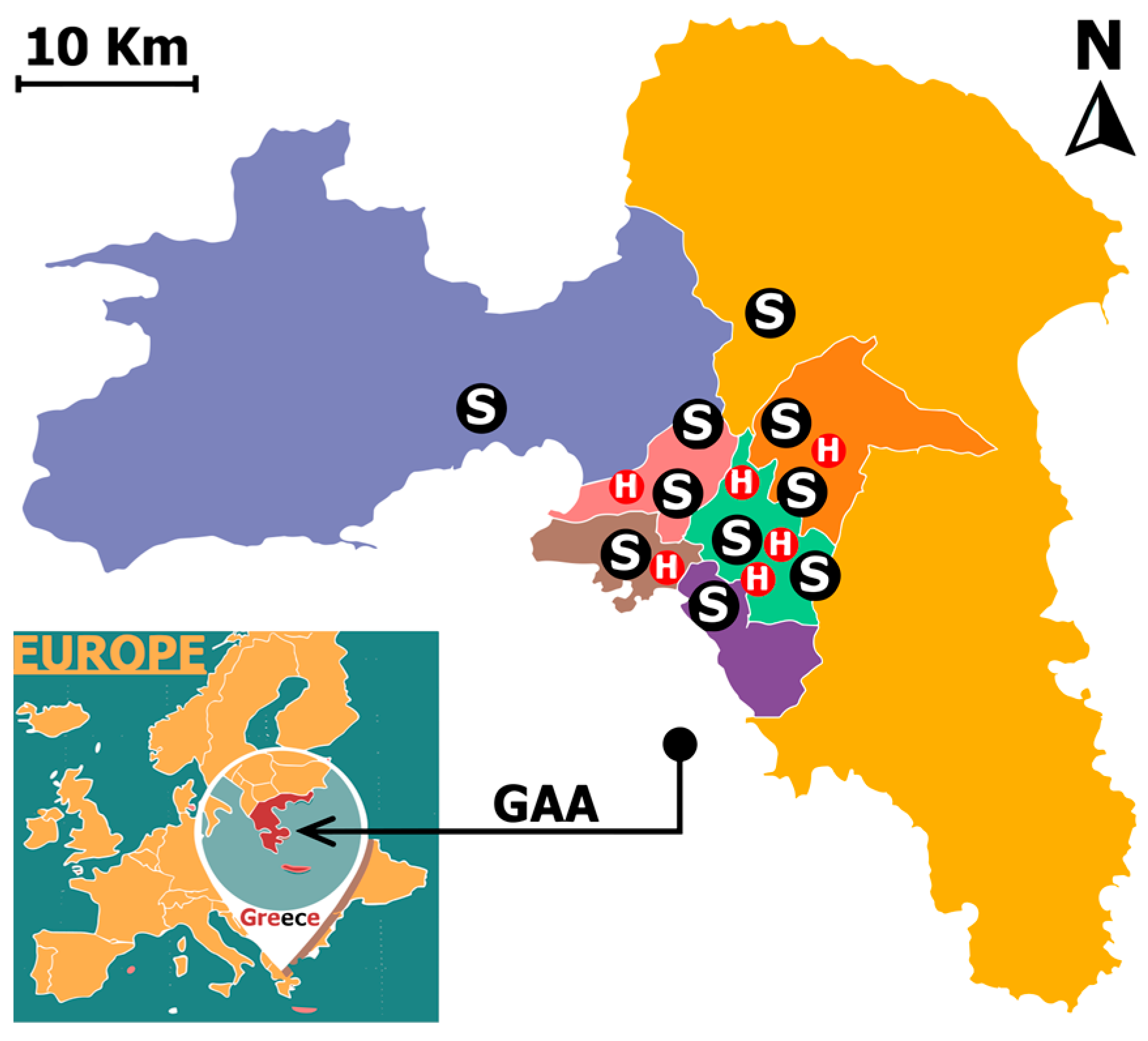
2.1. Study Area Characteristics

This study focuses on the Region of Attica, Greece, which includes the Greater Athens Area (GAA). The region has a population of approximately 3.79 million residents and is characterized by diverse landscapes and climatic conditions that contribute to fluctuating air quality and thermal comfort levels.

The primary sources of air pollutants in Attica include automobiles, industrial activities, and central heating, particularly during the colder months [31]. In 2020, approximately 4.4 million vehicles were in operation [32], leading to significant traffic congestion, exacerbated by an inefficient peripheral road network. This congestion remains a major contributor to photochemical pollutants, prompting local authorities to impose traffic restrictions based on vehicle registration numbers to mitigate pollution levels.

Industrial zones in the southwest of Athens and the Thriassion plain, along with emissions from the Piraeus harbor, contribute to regional pollution levels. These emissions, combined with prevailing atmospheric conditions (e.g., strong winter temperature inversions and sea–land breeze circulation), result in frequent air pollution episodes lasting from 3 to 5 days [33]. Despite these challenges, the air quality in Athens remains comparable to other European cities facing similar issues [33].

The region also experiences pronounced meteorological and thermal discomfort conditions, particularly during the warm season. Athens, located in the Mediterranean, is among the areas projected to experience significant increases in the frequency, intensity, and duration of heatwaves in both present and future climates [34,35,36]. Various methodologies, including absolute air temperature thresholds [37,38] and biometeorological indices [39,40], have been used to assess heatwave trends. Researchers have further analyzed heatwaves in Greek cities using the Excess Heat Factor index [41], highlighting the intensification of heat stress in the region.

Athens, and thus the GAA, has a typical Mediterranean climate, characterized by mild, wet winters and hot, dry summers [42]. During the warm period, strong north-northeasterly winds, known as ‘Etesians’, provide temporary relief from extreme heat, moderating temperatures and alleviating heat stress to some extent [43,44]. However, heatwaves, often exacerbated by Urban Heat Island effects, remain a critical concern, contributing to significant thermal discomfort and potential health impacts, particularly for vulnerable populations.

2.2. Data Collected

The data collected for this study covered the period from 2018 to 2022 and served as the exposure and response variables necessary for the model adopted to investigate the relationship between air pollution, meteorological conditions, and HAs. Specifically, daily hospital data were collected as the response variable, while hourly air pollution measurements and meteorological data (daily T, RH) were obtained from the national network of monitoring stations across the GAA, including Athens (ATH), Piraeus (PIR), Peristeri (PER), Elefsina (ELE), Maroussi (MAR), Thrakomakedones (THR), Agia Paraskevi (AGP), Lykovrisi (LYK), Nea Smyrni (NSM), and Liosia (LIO). All datasets were gathered by official public services, ensuring data reliability and standardization. However, to maintain data integrity, hospital admission records that lacked a precise location within the GAA were excluded as inconsistent. Additionally, meteorological and air pollution datasets were quality checked and cleared by their respective public agencies before analysis, ensuring accuracy and completeness. These datasets were then analyzed to assess their correlations and potential health impacts.

2.2.1. Hospital Admissions

The response variable HAs, specifically because of CVD and RD, were collected from six major hospitals in the GAA:

• Evaggelismos (EVA), Konstantopoulio (KON), and Elpis (ELP)—Central GAA Sector;
• Attikon (ATI)—West GAA Sector;
• Tzanio (TZA)—Piraeus (Southwest GAA);
• Sismanoglio (SIS)—North GAA Sector.

The selection of these hospitals was based on the following criteria:

✓

Data Availability and Consistency: Hospitals were chosen based on the availability of consistent admissions data covering the study period (2018–2022) to ensure robust analysis;

✓

Relevance to the Study: The selected hospitals include clinics specializing in RD and CVD, as these diseases are strongly linked to air pollution and temperature extremes;

✓

Public Healthcare System Representation: Only public hospitals were included to ensure access to a broad and diverse patient population, avoiding biases related to private healthcare access;

✓

Hospital Capacity and Regional Coverage: The six hospitals in the dataset collectively have a total bed capacity of 2907, which accounts for approximately 34% of the total bed capacity of public hospitals in Attica, standing at 8476 beds as of 2022 [45], ensuring adequate case volume for analysis.

Additionally, their geographic distribution covers all major regions of the GAA, ensuring regional representativeness.

These hospitals represent a broad geographical spread, ensuring comprehensive coverage of the region. During the five-year study period, a total of 64,044 HAs for CVDs and RDs were recorded, with approximately 60% related to RDs and 40% to CVD cases. These admissions collectively resulted in 469,844 hospital stays, indicating an average hospitalization duration of over a week per patient in these categories. This substantial burden highlights not only the direct health impacts of environmental factors, but also the considerable strain on healthcare resources and associated costs. The distribution of the hospitals across the Attica Region is shown in Figure 1, where the majority are located within the Attica Basin, with the exception of Attikon, which is situated in the Thriassion Plain to the west. Given the considerable number of hospitalizations linked to air quality-sensitive diseases, monitoring and controlling potential excess cases of HA is crucial. Effective public health interventions and environmental policies could play a key role in mitigating these impacts, reducing both the healthcare burden and the economic costs associated with prolonged hospital stays.

2.2.2. Air Quality Index Levels

The European Air Quality Index (EAQI) is an online tool developed by the European Environment Agency (EEA) that provides near real-time information on air quality across Europe. It integrates data from over 3500 monitoring stations, focusing on five critical pollutants: particulate matter (PM₁₀ and PM_2.5), ozone (O₃), nitrogen dioxide (NO₂), and sulfur dioxide (SO₂). The EAQI categorizes air quality into six classes, from “Good” to “Extremely Poor”, based on the pollutant with the highest concentration. This categorization helps to inform on potential health risks and offers recommendations for outdoor activities, especially for vulnerable groups.

In this study, data from 10 monitoring stations in Attica (Figure 1), operated by the Ministry of Environment and Energy (MEEN), were analyzed for the period 2018–2022. Hourly concentrations of O₃ and NO₂, and the moving 24 h averages for PM₁₀ and PM_2.5 were classified according to the EU AQI scale. For each pollutant, air quality categorized as ‘Good’ or ‘Fair’ was assigned a value of zero, indicating negligible health risk. For the remaining AQI categories, “Moderate” up to “Extremely Poor”, values were assigned within specific ranges using interpolation to reflect severity: (1–2] for “Moderate”, (2–3] for “Poor”, (3–4] for “Very Poor”, and (4–5] for “Extremely Poor”. This approach ensures a gradual and proportional representation of aggravating air quality.

The daily maximum AQI values were calculated based on the highest value across all pollutants for each day, resulting in a range from 0 to 5. To further refine the data, these values were categorized into levels based on pollutant concentration percentiles, as shown in the table below (Figure 2). Specifically, the “Moderate” and “Poor” AQI categories were divided into four equal parts using percentile ranges: 0–25th, 25th–50th, 50th–75th, and 75th–100th. The “Very Poor” AQI category was split into two levels based on percentiles, while the “Extremely Poor” category remained a single level due to its already severe pollution impact. The good and fair categories were combined into a single zero level, representing the threshold below which short-term air pollution impacts are considered negligible.

This structured classification allowed each day to be assigned a level from 0 to 11, named the Daily Maximum AQI Level (DMAQIL), reflecting the daily air quality and forming the basis for analyzing its impact on HAs. By segmenting air quality data into percentile-based sub-levels, the study was able to identify subtle variations in air pollution exposure and their correlation with health outcomes. This methodology provides a comprehensive approach for evaluating the health risks associated with air pollution in Attica, aiding in the development of targeted public health strategies.

2.2.3. Apparent Temperature

The meteorological data used in this study were obtained from ten meteorological stations operated by the METEO unit at the National Observatory of Athens [46], with their geographic distribution illustrated in Figure 1. The dataset includes hourly values of temperature, relative humidity, and wind speed, which were used to compute the Apparent Temperature (AT). In contrast to other studies that relied on hourly calculations, the AT in this study was determined separately for the warm and cold periods, to ultimately use the daily maximum and minimum values, respectively. The warm period is defined as April to September, while the cold period extends from October to March.

The AT was estimated following the Steadman formula [47], which accounts for the air temperature T in °C, vapor pressure VP in hPa (derived from the relative humidity and air temperature), and the wind speed u in m/s, to reflect the perceived thermal stress on the human body.

$$\mathrm{A}\mathrm{T}=\mathrm{T}+0.33\ast \mathrm{V}\mathrm{P}-0.7\ast \mathrm{u}-4.0$$

(1)

The computed values were then categorized into 19 levels regarding their percentile-based thresholds. Specifically, the warm period’s daily maximum AT was divided into levels 1 to 9, corresponding to percentile ranges from the 55th to the 95th, with the 55th percentile calculated at 21.3 °C. Conversely, the cold period’s daily minimum AT was categorized into levels −1 to −9, representing percentile ranges from the 45th to the 5th percentile, with the 45th percentile calculated at 11.44 °C. The intermediate range, spanning the 45th to 55th percentiles, serves as the baseline category where temperature-related health effects are assumed to be negligible.

This classification provides a framework for assessing the Daily Extreme Apparent Temperature Level (DEATL)’s impact on health outcomes. At a high absolute value of the DEATL, there were distinct patterns observed in the meteorological parameters (

Table 1. Daily Extreme Apparent Temperature Levels (DEATLs) along with the relative temperature ranges and percentiles. Corresponding ranges of temperature, vapor pressure, and wind velocity are displayed, out of which DEAT ranges are calculated.

DEATL	DEAT	Percentile	Temperature (°C)	Vapor Pressure (hPa)	Wind Velocity (m/s)
9	Over 37.24	Over 95th	31.6–44.4	8.1–31.2	0.0–4.5
8	35.78 to 37.24	90th–95th	30.1–40.1	9.6–30.6	0.0–5.4
7	34.54 to 35.78	85th–90th	28.7–39.2	7.5–31.9	0.0–5.8
6	33.17 to 34.54	80th–85th	27.8–38.2	7.2–31.1	0.0–6.3
5	31.74 to 33.17	75th–80th	26.6–37.9	9.1–29.9	0.0–7.6
4	29.62 to 31.74	70th–75th	24.8–36.3	6.0–29.7	0.0–8.9
3	27.89 to 29.62	65th–70th	23.2–36.0	4.8–27.7	0.0–9.8
2	24.73 to 27.89	60th–65th	21.1–35.8	4.9–26.8	0.0–13.0
1	21.31 to 24.73	55th–60th	18.6–31.8	5.4–24.1	0.0–16.1
0	14.50 to 21.31	50th–55th	13.6–30.9	4.5–22.9	0.0–17.0
0	11.44 to 14.50	45th–50th	11.2–24.3	3.6–17.8	0.0–13.4
−1	4.51 to 11.44	40th–45th	5.7–18.8	3.1–15.9	0.0–13.4
−2	2.33 to 4.51	35th–40th	3.8–14.6	3.1–11.5	0.0–13.9
−3	1.74 to 2.33	30th–35th	3.3–11.6	2.9–9.5	0.0–11.6
−4	1.51 to 1.74	25th–30th	3.1–10.5	3.4–9.1	0.0–9.4
−5	1.32 to 1.51	20th–25th	3.0–9.7	3.2–8.9	0.0–9.8
−6	1.17 to 1.32	15th–20th	2.9–9.8	3.2–9.8	0.0–10.3
−7	−0.27 to 1.17	10th–15th	1.6–12.4	2.5–10.4	0.0–16.1
−8	−2.45 to −0.27	5th–10th	−0.3–9.4	3.0–8.2	0.0–12.1
−9	Up to −2.45	Up to 5th	−6.5–6.9	0.0–7.9	0.0–13.9

). At high DEATL values, approaching level 9, the temperature exceeds 30 °C, with the vapor pressure reaching up to 31.2 hPa, indicating a high atmospheric moisture content. Meanwhile, the wind velocity remains low, often below 5 m/s, suggesting stagnant air conditions that exacerbate heat stress. In contrast, at low DEATL values, approaching level −9, the temperature drops to below −6.5 °C, the vapor pressure falls to 0–7.9 hPa, and the wind velocity increases, sometimes exceeding 10 m/s, intensifying cold stress. This contrast highlights that high temperatures are often accompanied by low wind velocity, whereas extreme cold conditions are linked to stronger winds, reinforcing their distinct impacts on human thermal discomfort (Table 1).

The use of percentile-based thresholds in defining AT extremes is aligned with previous research that has established strong associations between extreme temperature events and adverse health outcomes. Multiple studies have demonstrated that heat waves characterized by daily mean temperatures exceeding the 95th and 97.5th percentiles are linked to increased mortality risks, particularly during prolonged events lasting for three or more days [48]. Similar findings have been observed across various geographical regions, including multi-community studies spanning multiple countries [48]. Moreover, research focusing on Brazil has highlighted a higher risk of all-cause and non-accidental mortality under extreme heat conditions, reinforcing the significance of high-threshold percentile definitions [49].

Cold spells have also been associated with elevated mortality risks, particularly due to CVDs and cerebrovascular diseases. Extreme cold events defined at the 3rd percentile threshold have been found to significantly increase deaths from ischemic and hemorrhagic strokes, particularly among older populations [48]. Additional studies have identified heightened vulnerability among individuals with respiratory conditions, such as chronic obstructive pulmonary disease, during cold spells [50]. The increased mortality risk during both heat waves and cold spells is particularly pronounced among older adults, who exhibit reduced thermoregulatory capacity and greater susceptibility to physiological stressors linked to temperature extremes. This heightened vulnerability is further compounded by factors such as social isolation, pre-existing medical conditions, and medication use, all of which can impair the body’s ability to cope with extreme temperatures [51,52,53].

Extreme temperature events have been consistently associated with increases in CVD and RD mortality across multiple studies [54,55,56]. The effects of heat waves and cold spells on cause-specific mortality show significant variability, with heat waves predominantly impacting cerebrovascular diseases and ischemic strokes, while cold spells exhibit stronger associations with hemorrhagic stroke and ischemic heart disease [48]. Furthermore, studies have identified differential mortality risks based on heat wave intensity, with thresholds ranging from the 90th to 99th percentiles and durations spanning two to four days [22]. Similarly, cold spells have been defined using various percentile cutoffs, such as the 10th, 7.5th, and 5th percentiles, with durations of up to four consecutive days, demonstrating significant associations with non-accidental morbidity and mortality [57,58].

By adopting this classification, the analysis allows for a nuanced understanding of how different AT thresholds correspond to varying levels of health risk, contributing to the broader body of research on meteorology-related morbidity.

2.3. Distributed Lag Non-Linear Model (DLNM)

In this study, Distributed Lag Non-linear Models (DLNMs) were employed to evaluate the delayed effects of air pollution and thermal discomfort, represented by DMAQIL and DEATL, respectively, on HAs. This approach aligns with previous research on environmental exposures and health outcomes [22]. The effects are quantified using Relative Risk (RR), which measures the probability ratio of an event occurring in the exposed group compared to the non-exposed group [59]. An RR of 1 indicates no difference in risk between these groups, whereas an RR greater than 1 suggests an increased risk due to exposure, and an RR below 1 implies a protective effect.

DLNMs are particularly effective in capturing both the non-linear relationships and time-lagged impacts of exposure variables. This capability makes them superior to conventional models, which often fail to address the complexity of non-linear ER dynamics. The DLNM framework utilizes a cross-basis function to map the relationship between predictors and their lagged effects, offering a comprehensive analysis of exposure over time [60,61]. For this analysis, DLNMs were implemented using the R programming language, specifically leveraging the DLNM package (R version 4.2.3; R Foundation for Statistical Computing) [62]. Generalized non-linear models were applied, initially using a quasi-Poisson family guided by the Quasi Akaike Information Criterion (QAIC) to address overdispersion. However, model performance comparisons indicated that a Negative Binomial (NB) model provided a superior fit, as evidenced by lower Akaike Information Criterion (AIC) and Bayesian Information Criterion (BIC) values compared to both Poisson and Generalized Additive Models (GAMs) (

Table 2. Model performance comparison across key statistical metrics.

Parameters	Negative Binomial	Poisson	GAM
AIC	15,007.05	20,535.5	20,697.62
BIC	15,414.5	20,937.44	20,991.84
Dispersion parameter	1.123719	6.229468	6.22823
R	0.6051255	0.6087412	0.6078343
RMSE	14.39894	14.3544	13.93135
MAE	11.71858	11.69806	11.45116

). The NB model yielded an AIC of 15,007.05 and a BIC of 15,414.5, outperforming the Poisson (AIC = 20,535.5, BIC = 20,937.44) and GAMs (AIC = 20,697.62, BIC = 20,991.84).

The Poisson model exhibited significant overdispersion (dispersion parameter = 6.2295), indicating that it did not adequately capture the variability in the count data. In contrast, the Negative Binomial model (dispersion = 1.1237) effectively corrected for overdispersion, further validating its selection.

While the Generalized Additive Model (GAM) had slightly lower RMSE (13.9314) and MAE (11.4512) values than the NB model (RMSE = 14.3989, MAE = 11.7186), its higher AIC and BIC suggest that this marginal improvement in predictive accuracy came at the cost of increased model complexity. Furthermore, the correlation coefficient (R) for the GAM (0.6078) was comparable to the NB (0.6051) and Poisson (0.6087) models, reinforcing that overdispersion correction was the key improvement rather than any substantial gain in correlation strength. Given these findings, the Negative Binomial model was selected as the most appropriate approach for this analysis.

In environmental epidemiology, hospital admission data are often influenced by organizational variability such as staff scheduling, on-duty vs. off-duty days, weekdays vs. weekends, and reporting delays. These factors introduce random fluctuations that can obscure real associations with environmental exposures. To address this, a smoothing technique using an Asymmetric Epanechnikov (AE) kernel was applied that incorporates information from the current day and three subsequent days—a configuration that aligns with typical 4-day hospital “on duty” rotations observed in the GAA region. This approach is supported by similar findings in the recent literature [63], which emphasize the utility of asymmetric kernels in enhancing sensitivity to sustained health effects.

Compared to the baseline (Classical DLNM) without smoothing, the application of an AE kernel significantly enhanced model performance, as shown in

Table 3. Comparative model performance metrics for Classical DLNM vs. DLNM with AE kernel.

Parameters	Classical DLNM	DLNM + AE Kernel
AIC	15,007.05	12,152.64
BIC	15,414.5	12,559.68
Dispersion parameter	1.123719	1.094679
R	0.6051255	0.7931329
RMSE	14.39894	6.6336854
MAE	11.71858	5.3533178
MB	−0.00888	−0.00010
MFB	10.30241	2.086531

. This approach led to a substantially better fit and higher predictive accuracy, with noticeably lower error metrics and stronger alignment between observed and predicted values. A slight reduction in model dispersion further highlights the benefit of noise reduction, while still preserving much of the model’s sensitivity to acute environmental effects—acknowledging a modest trade-off in the magnitude of the most immediate response estimates. Overall, these findings support the value of incorporating asymmetric kernel smoothing to reveal more stable and interpretable ER patterns.

To assess short-term health impacts, various maximum lag periods were tested. Specifically, for DMAQIL, lags of 4 to 7 days were examined to capture the distributed lag effects of air pollution. For the DEATL and interaction term (defined as the product of the DMAQIL and DEATL), lags of 3 to 7 days were tested, considering temperature’s typically immediate effects (0–3 lag days), as supported by multiple studies [64,65,66,67]. Different degrees of freedom (df) for time and day of the year (doy) were evaluated, using the AIC to identify the optimal configuration. The final model incorporated the best-fitting maximum lags: 3 days for the DEATL, 5 days for the DMAQIL, and 7 days for the interaction term, while the degrees of freedom were set as specified in Equation (2).

$$\begin{array}{l}\mathrm{A}\mathrm{d}\mathrm{m}\mathrm{i}\mathrm{s}\mathrm{s}\mathrm{i}\mathrm{o}\mathrm{n}\mathrm{s}~\mathrm{D}\mathrm{M}\mathrm{A}\mathrm{Q}\mathrm{I}{\mathrm{L}}_{\mathrm{b}\mathrm{a}\mathrm{s}\mathrm{i}\mathrm{s}}+\mathrm{D}\mathrm{E}\mathrm{A}\mathrm{T}{\mathrm{L}}_{\mathrm{b}\mathrm{a}\mathrm{s}\mathrm{i}\mathrm{s}}+\mathrm{I}\mathrm{N}\mathrm{T}\mathrm{E}\mathrm{R}\mathrm{A}\mathrm{C}\mathrm{T}\mathrm{I}\mathrm{O}{\mathrm{N}}_{\mathrm{b}\mathrm{a}\mathrm{s}\mathrm{i}\mathrm{s}}+\\ \mathrm{n}\mathrm{s}\left(\mathrm{t}\mathrm{i}\mathrm{m}\mathrm{e},\mathrm{d}\mathrm{f}=6\ast 5\right)+\mathrm{d}\mathrm{o}\mathrm{w}+\mathrm{y}\mathrm{e}\mathrm{a}\mathrm{r}+\mathrm{n}\mathrm{s}\left(\mathrm{d}\mathrm{o}\mathrm{y},\mathrm{d}\mathrm{f}=6\right)\end{array}$$

(2)

DMAQIL_basis, DEATL_basis, and INTERACTION_basis represent the cross-basis functions for air pollution, temperature, and their interaction, respectively. Natural cubic splines, ns(time, df = 6 × 5) and ns(doy, df = 6), were applied to control for long-term trends and seasonality, while indicator variables accounted for the day of the week (dow) and year.

Exposure data, processed as the DMAQIL and DEATL, facilitated the analysis of the short-term effects on HAs. The maximum lag of 3 days for the DEATL minimized the AIC and BIC values, confirming its short-term influence. The optimal maximum lags for the DMAQIL and interaction term were 5 and 7 days, respectively, capturing both immediate and delayed health effects. Natural cubic splines were employed to describe both ER and lag–response functions, with knots placed at the 10th, 50th, and 90th percentiles of exposure variables and at equidistant points on the logarithmic scale of the lag period. This methodology allowed for a precise representation of ER relationships over time. Potential confounders, including the day of the week, long-term trends, and seasonality, were controlled using indicator variables and 6 degrees of freedom per year.

In addition to the interaction-based final model (Equation (2)), separate models were fitted for DMAQIL_basis and DEATL_basis according to the aforementioned configuration to examine the independent effects of the environmental stressors on HAs. The DLNM methodology, combined with the Negative Binomial framework, provided a detailed representation of exposure impacts, even in the presence of delayed effects. This comprehensive approach ensures a robust analysis of the relationship between environmental stressors and health outcomes, offering valuable insights for public health risk assessments.

3. Results

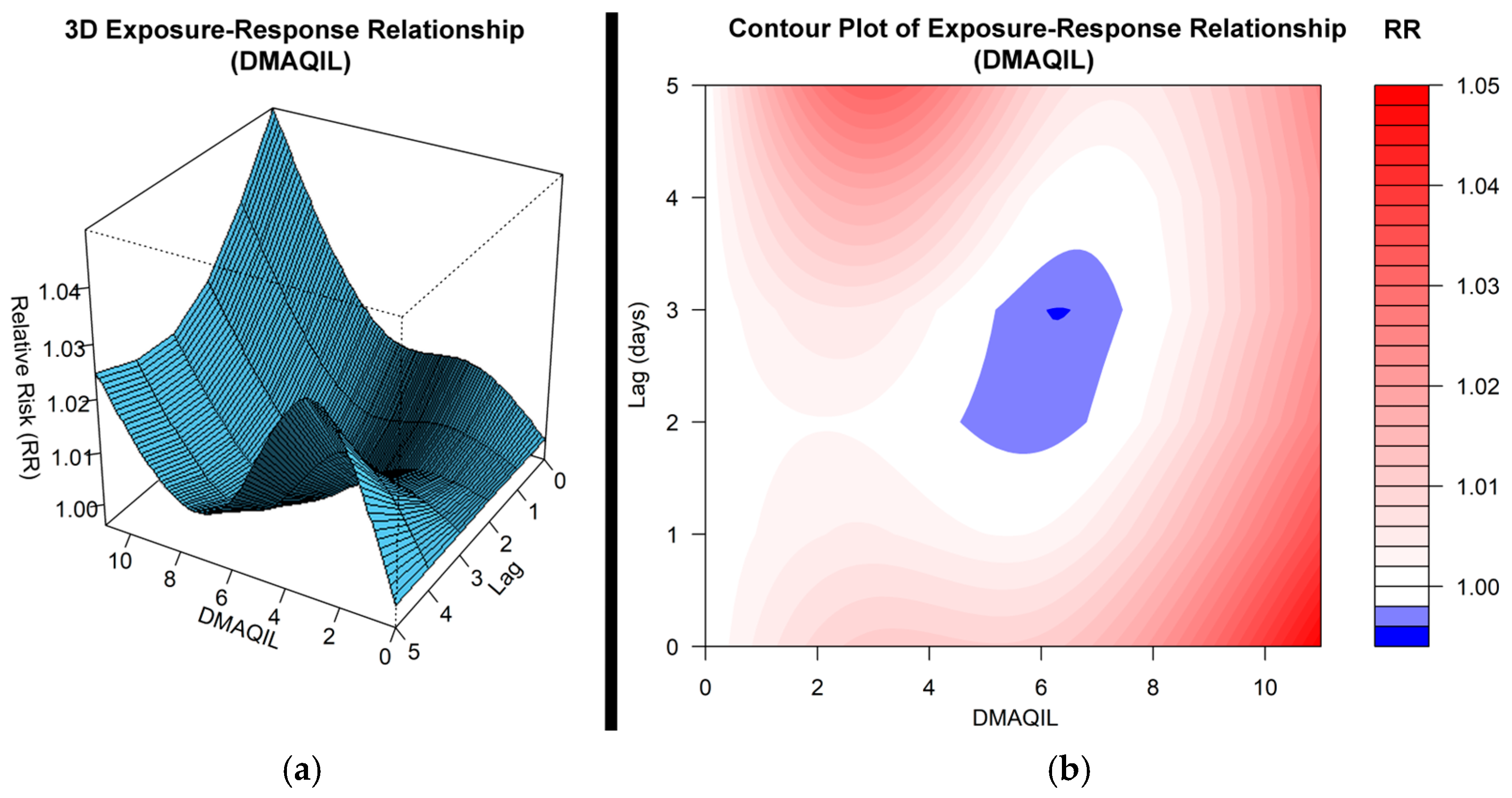
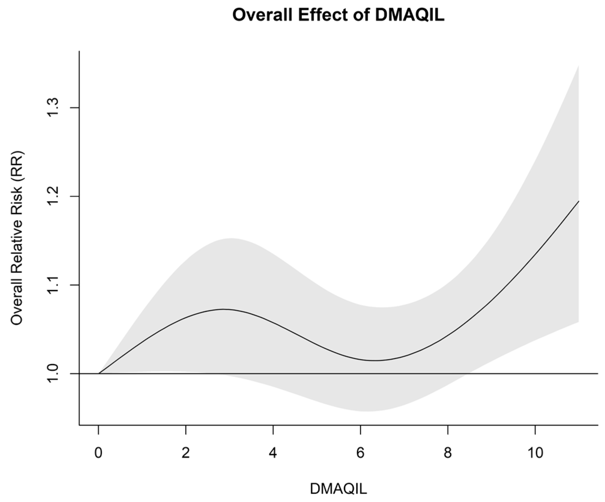
3.1. Impact of the DMAQIL on Hospital Admissions

Figure 3 displays the three-dimensional ER surface and the corresponding contour plot for the DMAQIL, derived from the independent DLNM analysis using the DMAQIL basis.

The most prominent peak appears at lag 0 for DMAQIL 11, where the RR reaches 1.050 (95% CI: 0.998–1.105). A second peak is observed at lag 1 for the same DMAQIL, with the RR at 1.037 (95% CI: 1.009–1.065). This upward trend continues across lags 2 to 5, where the RR remains elevated: at lag 2, the RR reaches 1.026 (95% CI: 0.994–1.060); and at lag 5, the RR peaks again at 1.025 (95% CI: 0.974–1.078).

Another notable increase is seen for the DMAQIL around 10, with the RR at 1.039 (95% CI: 1.000–1.079) at lag 0, and 1.027 (95% CI: 1.007–1.048) at lag 1. Additionally, for the DMAQIL around 9, there is a sustained rise across multiple lags: the RR reaches 1.029 (95% CI: 1.000–1.059) at lag 0, 1.018 (95% CI: 1.004–1.033) at lag 1, and 1.010 (95% CI: 0.992–1.028) at lag 2.

In contrast, the ER surface shows a mild decline in the RR for the DMAQIL values between 5 and 7, where the RR decreases to approximately 0.99 across lags 2 to 4.

These patterns highlight the dynamic short- and medium-term impacts of DMAQIL exposure, with acute effects emerging rapidly and additional responses extending across several lag days.

Figure 4 presents the overall effect of the DMAQIL on the RR, showing a distinct J-shaped pattern. At the lower end, the RR increases steadily from 1.000 at DMAQIL 0 to 1.036 at DMAQIL 1 (95% CI: 1.002–1.070). This upward trend continues, reaching 1.063 at DMAQIL 2 (95% CI: 1.002–1.128) and peaking around 1.072 at DMAQIL 3 (95% CI: 0.997–1.153). A gradual decline follows, with the RR tapering down through the mid-range: 1.058 at DMAQIL 4 (95% CI: 0.985–1.135) and dropping further to 1.033 at DMAQIL 5 (95% CI: 0.969–1.101). The lowest values occur at DMAQIL 6, where the RR reaches 1.016 (95% CI: 0.958–1.078), forming the bottom of the curve.

From DMAQIL 7 onward, the RR begins to climb again, reaching 1.020 at DMAQIL 7 (95% CI: 0.965–1.078) and 1.043 at DMAQIL 8 (95% CI: 0.987–1.102). This rising trend accelerates notably at higher DMAQIL values: the RR reaches 1.083 at DMAQIL 9 (95% CI: 1.014–1.156) and climbs sharply to 1.135 at DMAQIL 10 (95% CI: 1.038–1.241), culminating at 1.195 at DMAQIL 11 (95% CI: 1.058–1.348).

This overall trajectory illustrates a marked increase in risk at high air pollution levels, emphasizing the health burden associated with extreme DMAQIL exposures.

Figure 5 and Figure 6 present the frequency distribution of pollutant levels (PM₁₀, PM_2.5, O₃, and NO₂) across different DMAQIL categories, as well as their spatial distribution across various monitoring locations during the study period (2018–2022). Higher DMAQILs tend to be associated with more frequent occurrences of elevated PM₁₀ and PM_2.5 cases, particularly around DMAQIL 7 and 8. The O₃ levels show notable variability, with peak frequencies occurring around DMAQIL 5, while NO₂ demonstrates a declining pattern, with lower frequency counts at higher DMAQILs.

The absence of O₃ and NO₂ at DMAQILs between 9 and 11, despite the presence of PM₁₀ and PM_2.5, may be attributed to heterogeneous reactions occurring on particulate matter surfaces. Studies [68] have demonstrated that particulate matter can directly adsorb O₃ and facilitate redox reactions involving NO₂ and other nitrogen oxides (NO₃ and N₂O₅). Additionally, aerosol–photolysis feedback mechanisms can reduce photolysis rates, further limiting O₃ formation. These processes suggest that particulate matter not only persists, but actively modulates the concentrations of gaseous pollutants, supporting the observed trends in Figure 5.

In terms of the spatial distribution, station PIR records the highest frequencies of occurrences across most DMAQILs, particularly in mid-to-high ranges, suggesting that this area experiences a greater frequency of pollution events, which are attributed to NO₂, PM₁₀, and PM_2.5 levels. Conversely, locations such as PER, MAR, and AGP exhibit relatively lower frequencies across all DMAQILs. ATH and ELE show moderate frequencies, with noticeable increases at mid-range DMAQILs. This distribution highlights the variations in air pollution exposure across different regions during the study period.

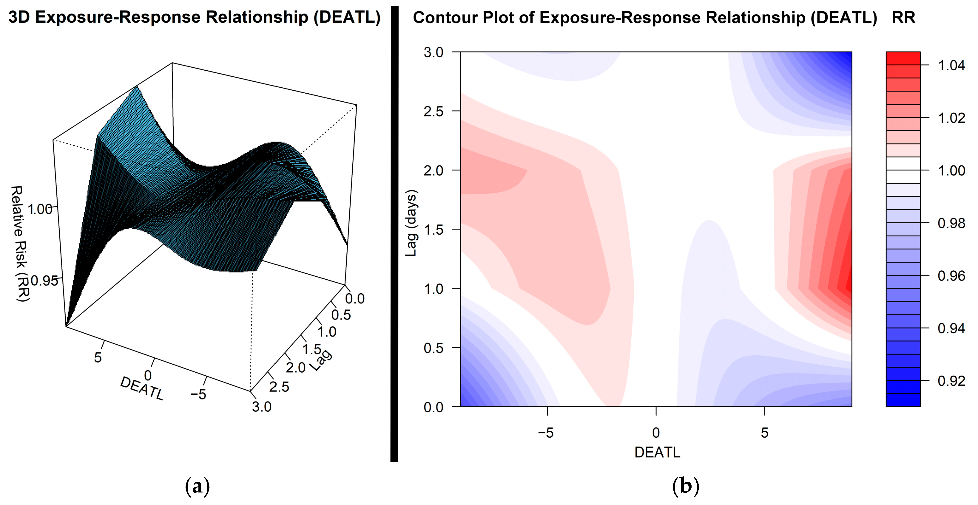
3.2. Impact of DEATL on Hospital Admissions

Figure 7 presents the three-dimensional ER relationship and the corresponding contour plot for the DEATL, based on the independent DLNM application of the DEATL_basis. The surface reveals three distinct peaks in the RR, two of which are notably associated with negative DEATL values.

The first and most prominent peak appears from lag 1 to lag 2 for DEATL values around −6 to −4, where the RR reaches approximately 1.014 (95% CI: 0.989–1.039) at lag 1 and DEATL −4. This zone indicates a consistent increase in the RR across lag 1 for moderately negative exposures. A second elevated region emerges for strongly negative DEATL values (around −9), particularly at lag 2, where the RR climbs to roughly 1.019 (95% CI: 0.987–1.053). This area marks a delayed risk response to extreme negative deviations in the DEATL.

The third and most sustained peak occurs at positive DEATL values, especially from lag 1 to lag 3. At lag 1 and DEATL 9, the RR reaches 1.044 (95% CI: 0.986–1.105), and at lag 2 and DEATL 9, it increases to 1.028 (95% CI: 0.970–1.088), reflecting a gradual and delayed increase in the RR under high exposure conditions.

In contrast, the contour plot shows a few blue regions indicating protective associations. The most pronounced decrease is seen at lag 3 and high DEATL values (8–9), where the RR drops to approximately 0.91. A more modest decline is also observed at lag 0 and DEATL −9, with the RR falling to around 0.94. These suggest both immediate and delayed protective effects at extreme values.

Figure 8 presents a bar chart illustrating the frequency of DEATLs across various levels (lvl_−9 to lvl_9) for all areas. A distinct pattern emerges, with ATH exhibiting the highest counts at positive levels (warm season), peaking at lvl_9 with 56 cases and maintaining high values from lvl_1 onward. In contrast, LIO records values only at negative levels (cold season), with a notable concentration at lvl_−9 (23 cases). ELE consistently shows zero counts across all levels, while NSM displays a distinct peak at lvl_0 (46 cases) and remains relatively high from lvl_1 to lvl_8. THR stands out with a significant presence at negative levels, particularly at lvl_−9 (51 cases) and lvl_−2 (53 cases), before gradually decreasing at higher levels. Meanwhile, AGP, MAR, PER, PIR, and LYK exhibit moderate fluctuations, with occasional peaks, such as PIR at lvl_5 (17 cases) and MAR at lvl_−7 (12 cases). Overall, the distribution indicates a shift in patterns, with certain regions showing a stronger presence at negative levels, while others peak at positive ones. These variations suggest potential regional differences, associated with the Urban Heat Island effect, in the underlying factors influencing the distribution of DEATLs across the level spectrum.

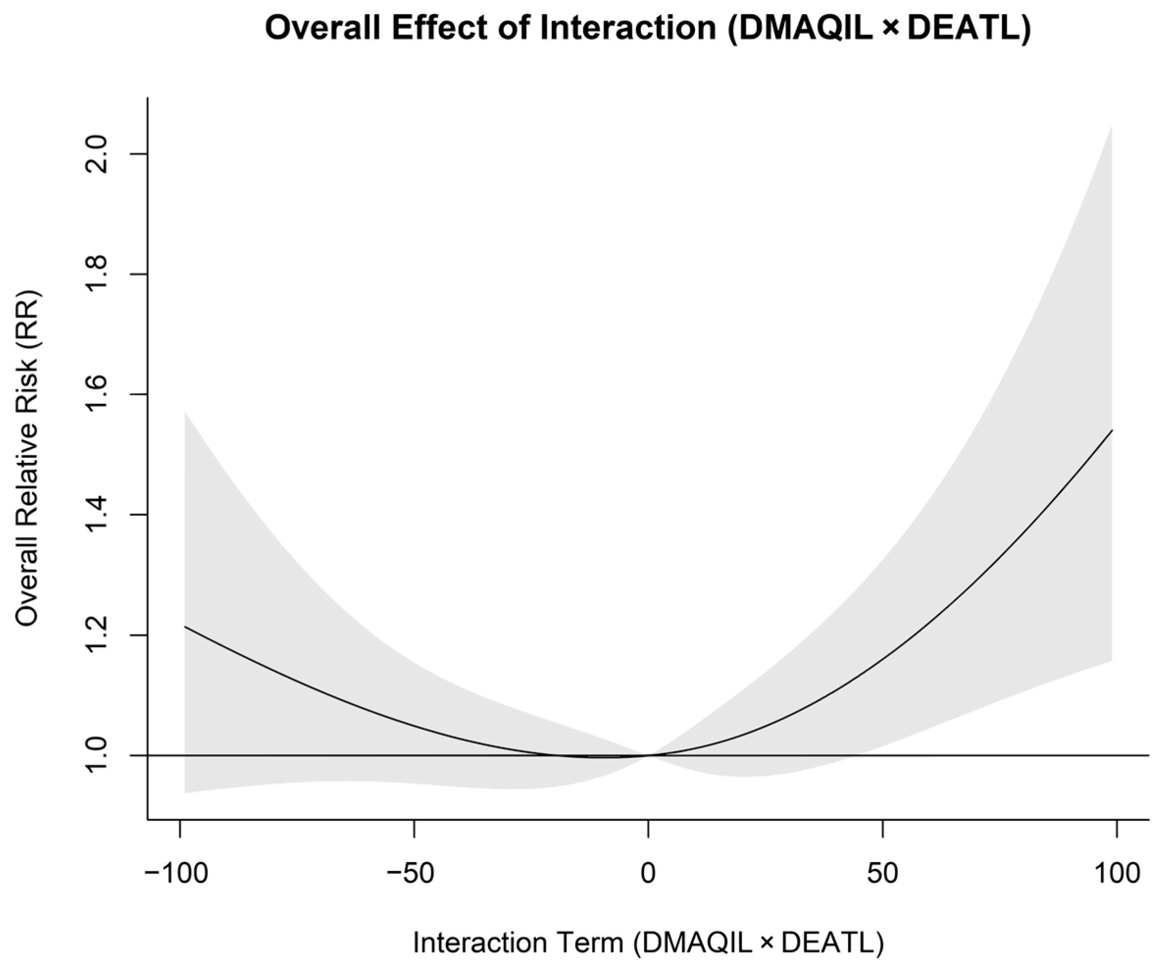
3.3. Impact of Interaction Term on Hospital Admissions

Figure 9 presents the 3D ER relationship and relative contour plot for the interaction term, derived from the final DLNM application (Equation (2)). A notable peak in the RR is evident when the interaction term goes beyond −15, with the RR increasing from 1.011 (95% CI: 0.994–1.027) to 1.154 (95% CI: 1.054–1.263) between lag 0 and just before lag 3, peaking at lag 0. A more pronounced rise is observed when the interaction term surpasses 25, where the RR escalates from 1.011 (95% CI: 0.994–1.028) to 1.152 (95% CI: 1.015–1.307) between lag 0 and just before lag 6, with the most substantial peak occurring around lag 0. Additionally, the contour plot reveals two blue spots, indicating a rapid decrease in the RR that follows after the corresponding red spots. The RR decreases to 0.94, with a faster decline observed in the spot that reaches the highest positive interaction values.

Figure 10 illustrates the overall RR in relation to the interaction term, showing a consistent and more pronounced increase when the interaction term exceeds +10. For negative interaction values beyond −30, such as −40 (approximately the 10th percentile), the RR is 1.027 (95% CI: 0.948–1.114), while at the extreme of −99 (0th percentile), the RR reaches 1.214 (95% CI: 0.937–1.572), indicating a gradual but notable elevation in the RR. However, the increase becomes more substantial in the positive range. For instance, at 20 (approximately the 75th percentile), the RR is 1.034 (95% CI: 0.965–1.109), while at the extreme value of 99 (100th percentile), the RR peaks at 1.540 (95% CI: 1.158–2.050). This pattern suggests that while both high negative and high positive interaction values are associated with an increased RR, the magnitude of risk becomes significantly higher as the interaction term surpasses +20, indicating a stronger synergistic effect in this direction.

4. Discussion

This study highlights significant associations between the DMAQIL, DEATL, and HAs, identifying distinct patterns in ER relationships and their temporal dynamics. The HA RR increases sharply at DMAQILs beyond 8, particularly around lag 0, and further intensifies even at low levels below 6 for lags 3–5. These findings suggest that air pollution thresholds trigger delayed health effects, where the impact of pollutants extends beyond the initial exposure period. The results align with prior research employing DLNMs that demonstrate similar delayed health effects [69,70,71].

Furthermore, the short-term nature of these effects supports findings that show that acute exposure to pollutants, particularly PM₁₀ and PM_2.5, has a direct and immediate impact on CVD and RD admissions [72,73]. This is further supported by Figure 5, which reveals that beyond DMAQIL 6, the contribution of particulate matter to air pollution increases, with PM_2.5 gradually becoming the dominant pollutant. This shift implies that at higher DMAQILs, the immediate and acute health impact of air pollution is largely driven by fine particulate matter. Given that PM_2.5 is smaller in size and can penetrate deeper into the respiratory and circulatory systems, its dominance at elevated DMAQILs may explain the rapid increase in HAs observed in this study. These findings align with the existing literature highlighting the heightened toxicity of PM_2.5 compared to larger particulates, reinforcing its role in triggering acute CVD and RD effects upon exposure [74,75,76].

Additionally, micron particles demonstrate enhanced deposition in stenotic regions when particle release velocities are low [77]. In this study, extreme positive DEATL values, which correspond to lower wind velocities, are associated with increased particle residence time and, consequently, higher deposition in critical areas of the respiratory system. Conversely, extreme negative DEATL values, indicative of higher velocities, tend to reduce particle deposition. This dynamic helps explain why the RR is greater during the warm season compared to the cold season. This observation further underscores the crucial role of meteorological conditions in modulating air pollution effects, highlighting the importance of considering these interactions when assessing health risks.

The findings reinforce those of previous studies [72], which emphasize that the air pollution effects on CVD are largely acute, underscoring the importance of short-term variations in pollutant exposure. Studies also indicate that the impact of pollutants on respiratory admissions is particularly pronounced in cold industrial regions, where lower temperatures contribute to temperature inversion, trapping pollutants in the atmosphere [78]. Strong correlations were observed between DMAQILs and pollution cases, particularly in industrial and densely populated regions such as PIR [79]. Additionally, significant associations between NO₂, PM₁₀, and ischemic stroke onset have been established [80], demonstrating how high pollution exposure increases ischemic stroke risk. These findings emphasize the need for targeted interventions in pollution hotspots. Moreover, the results corroborate earlier findings that pollutant interactions significantly modify health risks, with temperature changes influencing pollutant dispersion and modifying exposure levels [81].

The findings are consistent with previous research [82] in GAA, demonstrating that Black Smoke (BS) plays a dominant role in air pollution-related health outcomes, with a 10.2% increase in daily hospital admissions per 10 µg/m³ increase in PM₁₀ concentration. Similar associations were found for O₃, resulting in a 7.2% increase in daily hospital admissions per 10 µg/m³ increase. Moreover, meteorological factors such as temperature, wind velocity, and relative humidity were identified as critical determinants in estimating daily hospital admissions, emphasizing the complex interplay between meteorological conditions and air quality and its impact on health outcomes.

Similarly, the DEATL demonstrates a critical threshold effect, with HA risk increasing notably beyond level 5, along with additional peaks for values below −1. According to other research [83], the RR of mortality in Thessaloniki, Greece, was found to increase exponentially when the maximum Apparent Temperature exceeded 35 °C, which is close to DEATL 5, corresponding to 33 °C. This further supports the notion that extreme temperatures, both high and low, significantly impact health outcomes. Observed lagged effects for the DEATL confirm that extreme heat has a more immediate impact, a pattern also identified in previous research [84]. These results highlight the need for tailored response strategies focusing on immediate interventions to address heat-related health risks. These findings further reinforce the importance of acute responses to temperature fluctuations, aligning with the rapid increase in the RR observed when the DEATL surpassed level 5 within the first three days. Notably, studies have shown that exposure to extreme temperatures (>27 °C or <0.5 °C) significantly increases HAs for RD, with heat-related effects being more pronounced [78].

Another study conducted in Cyprus [85], using the daily mean temperature rather than the extreme AT, reported a U-shaped relationship between cardiorespiratory morbidity and temperature. Notably, health impacts were primarily associated with extreme cold, while the effects of extreme heat were comparatively modest.

The discrepancy between these findings and those from Cyprus likely stems from methodological differences. Unlike the daily mean temperature, the extreme Apparent Temperature used in this study is a more comprehensive meteorological metric, incorporating wind velocity and relative humidity. This allows for a more accurate assessment of temperature-related health impacts. Additionally, variations in local climate characteristics, pollution profiles, and population vulnerability between Greece and Cyprus may contribute to the observed differences.

Ozone is the dominant contributor at low DMAQILs, which also corresponds to a higher cumulative Relative Risk (RR), suggesting that ozone plays a key role in driving the elevated risk observed in these conditions. Notably, a study found increased mortality at 40–50 ppb (80–100 µg/m³), which falls within this range [86]. Additionally, other studies [87,88] linked a 10 ppb (19.6 µg/m³) ozone increase to 0.52–1.59% increases in daily mortality, reinforcing the idea that even small increases in low ozone concentrations can have measurable effects. These studies were conducted at mean ozone levels of 26 ppb (50.96 µg/m³) and 40.8 ppb (79.97 µg/m³), respectively, further highlighting the impact of relatively low ozone exposures on health. Similarly, others have identified a V-shaped relationship between O₃ and ischemic stroke onset [80], indicating that both high and low levels of O₃ may elevate health risks. These findings emphasize the need for comprehensive ER assessments that account for complex pollutant interactions.

Pollutant distribution analysis indicates that elevated DMAQILs correspond to PM₁₀ and PM_2.5 domination, whereas NO₂ exhibits a declining pattern at higher DMAQILs. Additionally, the spatial distribution of these pollutants emphasizes disproportionate exposure burdens in certain regions, with PIR recording the highest frequency of occurrences across most DMAQILs. The presence of blue spots across contour plots indicates temporary reductions in the RR, prior to or followed by peaks of increased HAs. These blue areas suggest several mechanisms, including the harvesting effect, delayed hospitalizations, risk absorption by other factors, and non-linear ER relationships. The pollutant distribution analysis indicates that elevated DMAQILs correspond to PM₁₀ and PM_2.5 domination, whereas NO₂ exhibits a declining pattern at higher DMAQILs. Additionally, the spatial distribution of these pollutants emphasizes disproportionate exposure burdens in certain regions, with PIR recording the highest frequency of occurrences across most DMAQILs. Another important aspect of this research is the presence of blue spots across contour plots, which indicate temporary reductions in RR, prior or followed by peaks of increased HA. These blue areas suggest several mechanisms, including the harvesting effect, delayed hospitalizations, risk absorption by other factors, and non-linear ER relationships.

The harvesting effect occurs when extreme weather or air pollution conditions accelerate adverse health outcomes among the most susceptible individuals, leading to short-term health impact displacement [89,90,91,92]. This phenomenon is particularly evident in CVD and stroke morbidity, where a surge in HAs or out-of-hospital deaths occurs early, followed by a subsequent drop in risk [74,93,94]. In Figure 9, where interaction effects are examined, the blue spots following red areas suggest harvesting, as vulnerable individuals are hospitalized early or succumb quickly, leading to a temporary decline in admissions. Similarly, in Figure 3 (DMAQIL contour plot), a sharp RR increase was observed at lag 0, as the DMAQIL surpasses 6, followed by a part of a blue spot, which aligns with previous studies identifying mortality displacement after acute exposure peaks [95,96].

Another reason for blue spots is delayed hospitalization and the avoidance of immediate medical attention. Cold-related illnesses often manifest later than heat-related conditions, contributing to temporary dips in the RR before subsequent increases in hospitalizations [93,97]. Certain populations, such as immigrants, individuals with complications, or those with limited access to healthcare, may delay hospitalization due to financial or systemic barriers [98,99]. In Figure 7 (DEATL contour plot), the blue spots at lag 0–1 (DEATL −9) suggest that cold-related admissions may be delayed, supported by studies where cold effects on CVD hospitalizations peaked at lag 10–12 [93,97]. Light blue areas appearing before a red peak, such as in Figure 3 at DMAQIL ~5, suggest that patients postpone hospital visits despite experiencing symptoms, which aligns with findings that some individuals delay care until symptoms worsen [75,76].

Additionally, protective behavioral responses can also lead to temporary reductions in the RR. Behavioral responses to extreme conditions such as staying indoors, using protective measures like masks or air purification, and reducing outdoor exposure, may mitigate exposure risk, leading to fewer HAs than expected [100,101]. In Figure 7 (DEATL contour plot), a rapid RR drop around DEATL 9 at lag 0 was found, likely due to high temperatures, prompting behavioral changes such as air conditioning use, hydration, and avoidance of outdoor exposure.

Another key observation is that the interaction term appears to absorb the RR at its highest absolute values, particularly at early lags. This pattern suggests that at extreme co-exposure levels, competing physiological mechanisms, behavioral adaptations, or even the initial depletion of the most vulnerable population may suppress HAs. Specifically, when the DEATL reaches its highest absolute values (8–9), even in combination with relatively low DMAQILs (around 3), its absolute product approaches 25, marking the threshold above which the interaction term begins to increase its RR, significantly, (as seen in Figure 9’s contour plot) at early lags. This dynamic may contribute to an initial decrease in the RR in the DEATL, reinforcing the idea that extreme conditions interact to create a short-term buffering effect before delayed health consequences emerge.

A similar attenuation effect is observed in Figure 4, in the DMAQIL range of 4–6, forming a distinct U-shaped pattern. This aligns with the blue spot in Figure 3, suggesting a temporary reduction in HAs at these moderate DMAQILs. Several explanations could account for this phenomenon. First, moderate pollution exposure might trigger short-term physiological adaptations, temporarily suppressing health impacts before cumulative effects take hold [75,102]. Second, risk attenuation due to non-linear ER relationships could contribute to this pattern, as observed in previous studies showing that moderate pollution levels do not always lead to significant health risks [75,102]. Third, environmental or behavioral factors may play a role, as moderate DMAQILs could coincide with meteorological conditions that mitigate pollution effects, or individuals may perceive air quality as tolerable and delay seeking medical attention [103,104].

The presence of this protective RR range reinforces the complexity of ER dynamics, highlighting the need for refined assessments that consider not only peak pollution levels, but also intermediate exposures and their interactions with meteorological conditions. This aligns with findings that show that short-term adjustments to extreme weather and pollution, such as reduced mobility, hydration, or medical interventions, can modulate immediate health effects before delayed physiological consequences manifest [102,104]. The present analysis further confirms that the interaction between air pollution and meteorology exacerbates health risks, extending the duration and severity of exposure effects [74,76,102]. In Figure 9, the RR increases significantly for both positive and negative interaction values, indicating that pollution-interactions lead to more sustained HAs compared to isolated factors [74,76]. The overall cumulative risk graphs (Figure 10) show that the interaction effects are of greater magnitude than those of air pollution alone, reinforcing findings that combined environmental exposures extend health risks over multiple days [103,104].

5. Conclusions

This study investigates the combined effects of air pollution and meteorological conditions on HAs in the GAA from 2018 to 2022, utilizing data from multiple monitoring locations and hospitals across the region. By analyzing ER relationships through the DLNM, how environmental stressors influence CVD and RD health risks over time was assessed.

The present analysis demonstrates novel insights into the ER relationships of the DMAQIL and DEATL, reinforcing previously observed trends while also identifying new patterns that warrant further investigation. Crucially, the interaction between meteorology and air pollution creates more acute, immediate, and prolonged health effects than individual exposures alone, underscoring the need for integrated public health strategies to mitigate these synergistic risks. The observed interaction term effects demonstrate a significantly greater cumulative impact than air pollution alone, further emphasizing that combined environmental stressors must be accounted for in assessing population health risks. Given the increasing frequency of extreme temperature events and persistent air pollution challenges, the findings of this study highlight the need for targeted public health interventions that prioritize real-time monitoring and adaptive response strategies to mitigate HA risks.

5.1. Policy and Hospital Recommendations

To mitigate the health impacts of air pollution and thermal stress, the analysis suggests several key interventions:

• Hospital Preparedness and Public Health Response
  • Hospitals should implement action protocols informed by advanced heat–health–air quality warning systems, allowing for proactive patient management during high-risk periods;
  • Emergency departments should be equipped with specialized protocols for handling heatstroke, respiratory distress, and cardiovascular exacerbations linked to environmental exposure;
  • Vulnerable populations, such as the elderly, children, and individuals with preexisting conditions, should be prioritized in hospital risk mitigation plans during extreme weather and pollution events.
• Air Quality and Urban Planning Policies
  • Policymakers should strengthen air quality regulations by enforcing stricter pollution control measures, particularly for industrial zones and traffic-congested areas, where air pollution is most severe;
  • Urban planning should integrate green infrastructure, such as vegetation barriers and urban forests, to reduce Urban Heat Island effects and improve air quality;
  • Public awareness campaigns should educate citizens about self-protection measures, such as avoiding outdoor activities during high pollution days and using air filtration systems indoors.

5.2. Implications for Environmental Regulations and Hospital Protocols

The analysis reveals that environmental regulations should consider the interactive effects of meteorology and air pollution, rather than assessing these factors in isolation. Future policies should focus on dynamic risk assessment models that integrate weather forecasting and air quality trends to better anticipate hospital admission surges. Additionally, hospital protocols should adopt climate-adaptive health strategies, ensuring that medical infrastructure is resilient to increasing climate variability and pollution-related health burdens.

5.3. Study Limitations and Potential Biases

While the current study provides valuable insights, several limitations must be acknowledged:

• Data quality and measurement bias: Air pollution and meteorological data were obtained from certain monitoring stations, which may not fully capture personal exposure levels or localized environmental variations within the GAA;
• Lack of individual and demographic data: The analysis was based on aggregated hospital admissions rather than individual health records, limiting the ability to control for demographic variations, preexisting medical conditions, socioeconomic factors, or lifestyle behaviors that could influence health risks;
• Potential reporting bias: The dataset excludes cases from private hospitals, which may lead to an incomplete representation of hospital admissions across different socioeconomic groups. Additionally, unreported cases of mild or untreated conditions could result in an underestimation of the true health burden;
• Confounding factors: While the model adjusts for seasonality and long-term trends, additional confounding factors, such as indoor air pollution, occupational exposures, or medication use, were not directly assessed;
• Higher-order Nonlinearities and model assumptions: Although the DLNM with the NB model was selected due to its strong fit and ability to handle overdispersion, GAMs are capable of capturing complex, non-linear relationships in the data. The slightly lower RMSE and MAE values for the GAM suggest that higher-order non-linear effects may exist, which the DLNM does not fully capture.

5.4. Future Research Directions

To enhance the understanding of environmental health risks, future studies should carry out the following:

• Integrate high-resolution patient data to assess individual susceptibility more accurately;
• Expand real-time environmental surveillance by deploying additional monitoring stations for better spatial coverage;
• Develop personalized health risk models that account for socioeconomic disparities in exposure and access to healthcare;
• Investigate potential synergies between pollutants to enhance the understanding of their individual and combined impacts on health outcomes;
• Future research could explore DLNM-GAM hybrid models to capture both the delayed and non-linear effects of environmental exposures while balancing flexibility with interpretability;
• While the current findings provide valuable insights, future studies could benefit from access to larger datasets and more granular hospital or exposure data to further reduce noise and uncertainty in the estimates. Additionally, incorporating machine learning techniques—such as random forests, gradient boosting, or neural networks—may further improve model efficiency by capturing complex, non-linear interactions that traditional approaches may miss. These techniques hold promise for enhancing predictive accuracy and uncovering more nuanced patterns in environmental health relationships.

By addressing these gaps, future research can further refine intervention strategies and improve climate-resilient public health responses.

References

1. Gao, J.H.; Woodward, A.; Vardoulakis, S.; Kovats, S.; Wilkinson, P.; Li, L.P.; Xu, L.; Li, J.; Yang, J.; Cao, L.; et al. Haze, public health and mitigation measures in China: A review of the current evidence for further policy response. Sci. Total Environ. 2017, 578, 148–157. [Google Scholar] [CrossRef]
2. European Environment Agency (EEA). Cutting Air Pollution in Europe Would Prevent Early Deaths, Improve Productivity and Curb Climate Change. Available online: https://www.eea.europa.eu/highlights/cutting-air-pollution-in-europe (accessed on 15 December 2024).
3. Duan, R.R.; Hao, K.; Yang, T. Air pollution and chronic obstructive pulmonary disease. Chronic Dis. Transl. Med. 2020, 6, 260–269. [Google Scholar] [CrossRef]
4. Jiang, X.Q.; Mei, X.D.; Feng, D. Air pollution and chronic airway diseases: What should people know and do? J. Thorac. Dis. 2016, 8, E31–E40. [Google Scholar] [PubMed]
5. Brunekreef, B.; Holgate, S.T. Air pollution and health. Lancet 2002, 360, 1233–1242. [Google Scholar] [CrossRef] [PubMed]
6. De Sario, M.; Katsoujanni, K.; Michelozzi, P. Climate change, extreme weather events, air pollution and respiratory health in Europe. Eur. Respir. J. Off. J. Eur. Soc. Clin. Respir. Physiol. 2013, 42, 826–843. [Google Scholar] [CrossRef]
7. USA EPA. Technical Assistance Document for the Reporting of Daily Air Quality—The Air Quality Index (AQI); Environmental Protection Agency: Washington, DC, USA, 2018.
8. Jiang, X.; Wei, P.; Luo, Y.; Li, Y.J.A. Air pollutant concentration prediction based on a CEEMDAN-FE-BiLSTM model. Atmosphere 2021, 12, 1452. [Google Scholar] [CrossRef]
9. Wang, J.; Du, P.; Hao, Y.; Ma, X.; Niu, T.; Yang, W. An innovative hybrid model based on outlier detection and correction algorithm and heuristic intelligent optimization algorithm for daily air quality index forecasting. J. Environ. Manag. 2020, 255, 109855. [Google Scholar] [CrossRef]
10. Li, H.; Wang, J.; Li, R.; Lu, H. Novel analysis—Forecast system based on multi-objective optimization for air quality index. J. Clean. Prod. 2019, 208, 1365–1383. [Google Scholar] [CrossRef]
11. Xie, Y.J.; Zhao, L.J.; Xue, J.; Gao, H.O.; Li, H.Y.; Jiang, R.; Qiu, X.Y.; Zhang, S.H. Methods for defining the scopes and priorities for joint prevention and control of air pollution regions based on data-mining technologies. J. Clean. Prod. 2018, 185, 912–921. [Google Scholar] [CrossRef]
12. Thunis, P.; Degraeuwe, B.; Pisoni, E.; Trombetti, M.; Peduzzi, E.; Belis, C.A.; Wilson, J.; Clappier, A.; Vignati, E. PM2.5 source allocation in European cities: A SHERPA modelling study. Atmos. Environ. 2018, 187, 93–106. [Google Scholar] [CrossRef]
13. Recast. European Parliament. 2024. Available online: https://eur-lex.europa.eu/eli/dir/2024/2881/oj/eng (accessed on 4 January 2025).
14. Poumadère, M.; Mays, C.; Le Mer, S.; Blong, R. The 2003 heat wave in France: Dangerous climate change here and now. Risk Anal. 2005, 25, 1483–1494. [Google Scholar] [CrossRef] [PubMed]
15. Cui, Y.; Ai, S.; Liu, Y.; Qian, Z.; Wang, C.; Sun, J.; Sun, X.; Zhang, S.; Syberg, K.M.; Howard, S.; et al. Hourly Associations Between Ambient Temperature and Emergency Ambulance Calls in One Central Chinese City: Call for an Immediate Emergency Plan. Sci. Total Environ. 2020, 711, 135046. [Google Scholar] [CrossRef]
16. Bhaskaran, K.; Armstrong, B.; Hajat, S.; Haines, A.; Wilkinson, P.; Smeeth, L. Heat and Risk of Myocardial Infarction: Hourly Level Case-Crossover Analysis of MINAP Database. BMJ 2012, 345, e8050. [Google Scholar] [CrossRef]
17. Liu, Y.; Kan, H.; Xu, J.; Rogers, D.; Peng, L.; Ye, X.; Chen, R.; Zhang, Y.; Wang, W. Temporal Relationship Between Hospital Admissions for Pneumonia and Weather Conditions in Shanghai, China: A Time-Series Analysis. BMJ Open 2014, 4, e004961. [Google Scholar] [CrossRef] [PubMed]
18. Kladakis, A.; Fameli, K.-M.; Moustris, K.; Assimakopoulos, V.D.; Nastos, P. Investigation into Atmospheric Pollution Impacts on Hospital Admissions in Attica Using Regression Models. Environ. Sci. Proc. 2023, 26, 25. [Google Scholar]
19. Parliari, D.; Economou, T.; Giannaros, C.; Kushta, J.; Melas, D.; Matzarakis, A.; Lelieveld, J. A comprehensive approach for assessing synergistic impact of air quality and thermal conditions on mortality: The case of Thessaloniki, Greece. Urban. Clim. 2024, 56, 102088. [Google Scholar] [CrossRef]
20. Schwartz, J. The distributed lag between air pollution and daily deaths. Epidemiology 2000, 11, 320–326. [Google Scholar] [CrossRef]
21. Gasparrini, A.; Leone, M. Attributable risk from distributed lag models. BMC Med. Res. Methodol. 2014, 14, 55. [Google Scholar] [CrossRef]
22. Singh, N.; Area, A.; Breitner, S.; Zhang, S.; Agewall, S.; Schikowski, T.; Schneider, A. Heat and Cardiovascular Mortality: An Epidemiological Perspective. Circ. Res. 2024, 134, 1098–1112. [Google Scholar] [CrossRef]
23. Joshi, M.; Goraya, H.; Joshi, A.; Bartter, T. Climate change and respiratory diseases. Curr. Opin. Pulm. Med. 2020, 26, 119–127. [Google Scholar] [CrossRef]
24. Katsouyanni, K.; Analitis, A. Investigating the Synergistic Effects Between Meteorological Variables and Air Pollutants: Results from the European PHEWE, EUROHEAT and CIRCE Projects. Epidemiology 2009, 20, S264. [Google Scholar] [CrossRef]
25. Analitis, A.; Donato, F.D.; Scortichini, M.; Lanki, T.; Basagana, X.; Ballester, F.; Astrom, C.; Paldy, A.; Pascal, M.; Gasparrini, A.; et al. Synergistic Effects of Ambient Temperature and Air Pollution on Health in Europe: Results from the PHASE Project. Int. J. Environ. Res. Public. Health 2018, 15, 1856. [Google Scholar] [CrossRef] [PubMed]
26. Lepeule, J.; Litonjua, A.A.; Gasparrini, A.; Koutrakis, P.; Sparrow, D.; Vokonas, P.S.; Schwartz, J. Lung function association with outdoor temperature and relative humidity and its interaction with air pollution in the elderly. Environ. Res. 2018, 165, 110–117. [Google Scholar] [CrossRef] [PubMed]
27. Jiang, Y.; Chen, R.; Kan, H. The Interaction of Ambient Temperature and Air Pollution in China. In Ambient Temperature and Health in China; Springer Nature: Singapore, 2019; pp. 105–116. [Google Scholar]
28. Krug, A.; Fenner, D.; Holtmann, A.; Scherer, D. Occurrence and Coupling of Heat and Ozone Events and Their Relation to Mortality Rates in Berlin, Germany, Between 2000 and 2014. Atmosphere 2019, 10, 348. [Google Scholar] [CrossRef]
29. Ryti, N.; Guo, Y.; Jaakkola, J. Global Association of Cold Spells and Adverse Health Effects: A Systematic Review and Meta-Analysis. Environ. Health Perspect. 2016, 124, 12–22. [Google Scholar] [CrossRef]
30. Pozzer, A.; Anenberg, S.C.; Dey, S.; Haines, A.; Lelieveld, J.; Chowdhury, S. Mortality attributable to ambient air pollution: A review of global estimates. GeoHealth 2023, 7, e2022GH000711. [Google Scholar] [CrossRef]
31. Fameli, K.-M.; Assimakopoulos, V.D. The New Open Flexible Emission Inventory for Greece and the Greater Athens Area (FEI-GREGAA): Account of Pollutant Sources and Their Importance from 2006 to 2012. Atmos. Environ. 2016, 137, 17–37. [Google Scholar] [CrossRef]
32. Chaziris, A.; Yannis, G. A critical assessment of Athens Traffic Restrictions using multiple data sources. Transp. Res. Procedia 2022, 72, 375–382. [Google Scholar] [CrossRef]
33. Kallos, G.; Kassomenos, P.; Pielke, R.A. Synoptic and mesoscale weather conditions during air pollution episodes in Athens, Greece. Bound. Layer. Meteorol 1993, 62, 163–184. [Google Scholar] [CrossRef]
34. Kuglitsch, F.G.; Toreti, A.; Xoplaki, E.; Della-Marta, P.M.; Zerefos, C.S.; Türke¸s, M.; Luterbacher, J. Heat wave changes in the eastern Mediterranean since 1960. Geophys. Res. Lett. 2010, 37, L04802. [Google Scholar] [CrossRef]
35. Diffenbaugh, N.S.; Pal, J.S.; Giorgi, F.; Gao, X. Heat stress intensification in the Mediterranean climate change hotspot. Geophys. Res. Lett. 2007, 34, L11706. [Google Scholar] [CrossRef]
36. Ouzeau, G.; Soubeyroux, J.M.; Schneider, M.; Vautard, R.; Planton, S. Heat waves analysis over France in present and future climate: Application of a new method on the EURO-CORDEX ensemble. Clim. Serv. 2016, 4, 1–12. [Google Scholar] [CrossRef]
37. Founda, D. Evolution of the air temperature in Athens and evidence of climatic change: A review. Adv. Build. Energy Res. 2011, 5, 7–41. [Google Scholar] [CrossRef]
38. Founda, D.; Giannakopoulos, C. The exceptionally hot summer of 2007 in Athens, Greece—A typical summer in the future climate? Glob. Planet. Chang. 2009, 67, 227–236. [Google Scholar] [CrossRef]
39. Matzarakis, A.; Nastos, P.T. Human-biometeorological assessment of heat waves in Athens. Theor. Appl. Climatol. 2011, 105, 99–106. [Google Scholar] [CrossRef]
40. Nastos, P.T.; Matzarakis, A. The effect of air temperature and human thermal indices on mortality in Athens, Greece. Theor. Appl. Climatol. 2012, 108, 591–599. [Google Scholar] [CrossRef]
41. Tolika, K. Assessing Heat Waves over Greece Using the Excess Heat Factor (EHF). Climate 2019, 7, 9. [Google Scholar] [CrossRef]
42. Peel, M.C.; Finlayson, B.L.; McMahon, T.A. Updated world map of the Köppen-Geiger climate classification. Hydrol. Earth Syst. Sci. 2007, 11, 1633–1644. [Google Scholar] [CrossRef]
43. Giannaros, C.; Agathangelidis, I.; Papavasileiou, G.; Galanaki, E.; Kotroni, V.; Lagouvardos, K.; Giannaros, T.M.; Cartalis, C.; Matzarakis, A. The extreme heat wave of July–August 2021 in the Athens urban area (Greece): Atmospheric and human-biometeorological analysis exploiting ultra-high resolution numerical modeling and the local climate zone framework. Sci. Total Environ. 2023, 857, 159300. [Google Scholar] [CrossRef]
44. Giannaros, C.; Economou, T.; Parliari, D.; Galanaki, E.; Kotroni, V.; Lagouvardos, K.; Matzarakis, A. A thermo-physiologically consistent approach for studying the heat-health nexus with hierarchical generalized additive modelling: Application in Athens urban area (Greece). Urban Clim. 2024, 857, 159300. [Google Scholar] [CrossRef]
45. Ministry of Health. Hospital Admissions and Hospital Beds. Available online: https://www.moh.gov.gr/articles/bihealth/stoixeia-noshleytikhs-kinhshs/10431-klines-noshleythentes-hmeres-noshleias-2021 (accessed on 20 December 2024).
46. Lagouvardos, K.; Kotroni, V.; Bezes, A.; Koletsis, I.; Kopania, T.; Mazarakis, N.; Papagiannaki, K.; Vougioukas, S. The automatic weather stations NOANN network of the National Observatory of Athens: Operation and database. Geosci. Data J. 2017, 4, 4–16. [Google Scholar] [CrossRef]
47. Steadman, R.G. A Universal Scale of Apparent Temperature. J. Clim. Appl. Meteorol. 1984, 23, 1674–1687. [Google Scholar] [CrossRef]
48. Moraes, S.L.; Almendra, R.; Barrozo, L.V. Impact of heat waves and cold spells on cause-specific mortality in the city of São Paulo, Brazil. Int. J. Hyg. Environ. Health 2022, 239, 113861. [Google Scholar] [CrossRef]
49. Guo, Y.; Gasparrini, A.; Armstrong, B.G.; Tawatsupa, B.; Tobias, A.; Lavigne, E.; Coelho, M.S.Z.S.; Pan, X.; Kim, H.; Hashizume, M.; et al. Heat Wave and Mortality: A Multicountry, Multicommunity Study. Environ. Health Perspect. 2017, 125, 087006. [Google Scholar] [CrossRef]
50. Chen, J.; Yang, J.; Zhou, M.; Yin, P.; Wang, B.; Liu, J.; Chen, Z.; Song, X.; Ou, C.Q.; Liu, Q. Cold spell and mortality in 31 Chinese capital cities: Definitions, vulnerability and implications. Environ. Int. 2019, 128, 271–278. [Google Scholar] [CrossRef]
51. Balmain, B.N.; Sabapathy, S.; Louis, M.; Morris, N.R. Aging and Thermoregulatory Control: The Clinical Implications of Exercising under Heat Stress in Older Individuals. Biomed Res. Int. 2018, 8306154. [Google Scholar] [CrossRef]
52. Kenny, G.P.; Yardley, J.; Brown, C.; Mph, R.J.S.; Jay, O. Heat stress in older individuals and patients with common chronic diseases. CMAJ 2010, 182, 1053–1060. [Google Scholar] [CrossRef]
53. Tansey, E.A.; Johnson, C.D. Recent advances in thermoregulation. Adv. Physiol. Educ. 2014, 39, 139–148. [Google Scholar] [CrossRef] [PubMed]
54. Anderson, B.G.; Bell, M.L. Weather-Related Mortality: How Heat, Cold, and Heat Waves Affect Mortality in the United States. Epidemiology 2009, 20, 205–213. [Google Scholar] [CrossRef]
55. Cheng, J.; Xu, Z.; Bambrick, H.; Prescott, V.; Wang, N.; Zhang, Y.; Su, H.; Tong, S.; Hu, W. Cardiorespiratory effects of heatwaves: A systematic review and meta-analysis of global epidemiological evidence. Environ. Res. J. 2019, 177, 108610. [Google Scholar] [CrossRef]
56. Fouillet, A.; Rey, G.; Laurent, F.; Pavillon, G.; Bellec, S.; Guihenneuc-Jouyaux, C.; Clavel, J.; Jougla, E.; Hémon, D. Excess mortality related to the August 2003 heat wave in France. Int. Arch. Occup. Environ. Health 2006, 80, 16–24. [Google Scholar] [CrossRef] [PubMed]
57. Feng, J.; Cao, D.; Zheng, D.; Qian, Z.; Huang, C.; Shen, H.; Liu, Y.; Liu, Q.; Sun, J.; Jiao, G.; et al. Cold spells linked with respiratory disease hospitalization, length of hospital stay, and hospital expenses: Exploring cumulative and harvesting effects. Sci. Total Environ. 2023, 863, 160726. [Google Scholar] [CrossRef]
58. Ning, Z.; He, S.; Liao, X.; Ma, C.; Wu, J. Health impacts of a cold wave and its economic loss assessment in China’s high-altitude city, Xining. Arch. Public Health 2024, 82, 52. [Google Scholar] [CrossRef]
59. Simon, S.D. Understanding the odds ratio and the relative risk. J. Androl. 2001, 22, 533–536. [Google Scholar] [CrossRef] [PubMed]
60. Gasparrini, A. Modeling exposure-lag-response associations with distributed lag non-linear models. Stat. Med. 2014, 33, 881–899. [Google Scholar] [CrossRef]
61. Gasparrini, A.; Armstrong, B.; Kenward, M.G. Distributed lag non-linear models. Stat. Med. 2010, 29, 2224–2234. [Google Scholar] [CrossRef]
62. Gasparrini, A. Distributed lag linear and non-linear models in R: The package dlnm. J. Stat. Softw. 2011, 43, 1–20. [Google Scholar] [CrossRef] [PubMed]
63. Masselot, P.; Chebana, F.; Bélanger, D.; St-Hilaire, A.; Abdous, B.; Gosselin, P.; Ouarda, T.B.M.J. Aggregating the response in time series regression models, applied to weather-related cardiovascular mortality. Sci. Total Environ. 2018, 628, 217–225. [Google Scholar] [CrossRef]
64. Rahman, M.M.; McConnell, R.; Schlaerth, H.; Ko, J.; Silva, S.; Lurmann, F.W.; Palinkas, L.; Johnston, J.; Hurlburt, M.; Yin, H.; et al. The Effects of Coexposure to Extremes of Heat and Particulate Air Pollution on Mortality in California: Implications for Climate Change. Am. J. Respir. Crit. Care Med. 2022, 206, 1117–1127. [Google Scholar] [CrossRef]
65. Rai, M.; Stafoggia, M.; de’Donato, F.; Scortichini, M.; Zafeiratou, S.; Vazquez Fernandez, L.; Zhang, S.; Katsouyanni, K.; Samoli, E.; Rao, S.; et al. Heat-related cardiorespiratory mortality: Effect modification by air pollution across 482 cities from 24 countries. Environ. Int. 2023, 174, 107825. [Google Scholar] [CrossRef]
66. Xia, Y.; Shi, C.; Li, Y.; Jiang, X.; Ruan, S.; Gao, X.; Chen, Y.; Huang, W.; Li, M.; Xue, R.; et al. Effects of ambient temperature on mortality among elderly residents of Chengdu city in Southwest China, 2016-2020: A distributed-lag non-linear time series analysis. BMC Public. Health. 2023, 23, 149. [Google Scholar] [CrossRef] [PubMed]
67. Zhang, S.; Breitner, S.; Rai, M.; Nikolaou, N.; Stafoggia, M.; De’ Donato, F.; Samoli, E.; Zafeiratou, S.; Katsouyanni, K.; Rao, S.; et al. Assessment of short-term heat effects on cardiovascular mortality and vulnerability factors using small area data in Europe. Environ. Int. 2023, 179, 108154. [Google Scholar] [CrossRef] [PubMed]
68. Qu, Y.; Wang, T.; Yuan, C.; Wu, H.; Gao, L.; Huang, C.; Li, Y.; Li, M.; Xie, M. The underlying mechanisms of PM2.5 and O3 synergistic pollution in East China: Photochemical and heterogeneous interactions. Sci. Total Environ. 2023, 873, 162434. [Google Scholar] [CrossRef]
69. Allen, M.J.; Sheridan, S.C. Mortality risks during extreme temperature events (ETEs) using a distributed lag non-linear model. Int. J. Biometeorol. 2015, 62, 57–67. [Google Scholar] [CrossRef] [PubMed]
70. Li, A.; Fan, L.; Xie, L.; Ren, Y.; Li, L. Associations between air pollution, climate factors and outpatient visits for eczema in West China Hospital, Chengdu, south-western China: A time series analysis. J Eur Acad. Dermatology Venereol. 2018, 32, 486–494. [Google Scholar] [CrossRef]
71. Petkova, E.P.; Gasparrini, A.; Kinney, P.L. Heat and mortality in New York city since the beginning of the 20th century. Epidemiology 2014, 25, 554–560. [Google Scholar] [CrossRef]
72. Martins, L.C.; Pereira, L.A.; Lin, C.A.; Santos, U.P.; Prioli, G.; Luiz, O.C.; Saldiva, P.H.; Braga, A.L. The effects of air pollution on cardiovascular diseases: Lag structures. Rev. Saude Publica 2006, 40, 677–683. [Google Scholar] [CrossRef]
73. Pothirat, C.; Chaiwong, W.; Liwsrisakun, C.; Bumroongkit, C.; Deesomchok, A.; Theerakittikul, T.; Limsukon, A.; Tajarernmuang, P.; Phetsuk, N. Acute effects of air pollutants on daily mortality and hospitalizations due to cardiovascular and respiratory diseases. J. Thorac. Dis. 2019, 11, 3070–3083. [Google Scholar] [CrossRef]
74. Yang, C.; Lei, L.; Li, Y.; Huang, C.; Chen, K.; Bao, J. Bidirectional modification effects on nonlinear associations of summer temperature and air pollution with first-ever stroke morbidity. Ecotoxicol. Environ. Saf. 2024, 272, 116034. [Google Scholar] [CrossRef]
75. Yang, L.; Yang, J.; Liu, M.; Sun, X.; Li, T.; Guo, Y.; Hu, K.; Bell, M.L.; Cheng, Q.; Kan, H.; et al. Nonlinear effect of air pollution on adult pneumonia hospital visits in the coastal city of Qingdao, China: A time-series analysis. Environ. Res. 2022, 209, 112754. [Google Scholar] [CrossRef]
76. Pan, K.; Lin, F.; Huang, K.; Zeng, S.; Guo, M.; Cao, J.; Dong, H.; Wei, J.; Xi, Q. The effect of short-term exposure to air pollution on the admission of ischemic stroke and its interaction with meteorological factors. Public. Health 2025, 239, 103–111. [Google Scholar] [CrossRef] [PubMed]
77. Gosman, R.E.; Sicard, R.M.; Cohen, S.M.; Frank-Ito, D.O. A computational analysis on the impact of multilevel laryngotracheal stenosis on airflow and drug particle dynamics in the upper airway. Exp. Comput. Multiph. Flow. 2023, 5, 235–246. [Google Scholar] [CrossRef] [PubMed]
78. Jia, H.; Xu, J.; Ning, L.; Feng, T.; Cao, P.; Gao, S.; Shang, P.; Yu, X. Ambient air pollution, temperature and hospital admissions due to respiratory diseases in a cold, industrial city. J. Glob. Health 2022, 12, 04085. [Google Scholar] [CrossRef]
79. euPOLIS Project. City of Piraeus. Available online: https://eupolis-project.eu/project/city-of-piraeus/ (accessed on 15 January 2025).
80. Wang, Z.; Peng, J.; Liu, P.; Duan, Y.; Huang, S.; Wen, Y.; Liao, Y.; Li, H.; Yan, S.; Cheng, J.; et al. Association between short-term exposure to air pollution and ischemic stroke onset: A time-stratified case-crossover analysis using a distributed lag nonlinear model in Shenzhen, China. Environ. Health A Glob. Access Sci. Source 2020, 19, 1. [Google Scholar] [CrossRef]
81. Wu, Z.; Miao, C.; Li, H.; Wu, S.; Gao, H.; Liu, W.; Li, W.; Xu, L.; Liu, G.; Zhu, Y. The lag-effects of meteorological factors and air pollutants on child respiratory diseases in Fuzhou, China. J. Glob. Health 2022, 12, 11010. [Google Scholar] [CrossRef] [PubMed]
82. Kassomenos, P.; Papaloukas, C.; Petrakis, M.; Karakitsios, S. Assessment and prediction of short term hospital admissions: The case of Athens, Greece. Atmos. Environ. 2008, 42, 7078–7086. [Google Scholar] [CrossRef]
83. Parliari, D.; Cheristanidis, S.; Giannaros, C.; Keppas, S.C.; Papadogiannaki, S.; de’Donato, F.; Sarras, C.; Melas, D. Short-Term Effects of Apparent Temperature on Cause-Specific Mortality in the Urban Area of Thessaloniki, Greece. Atmosphere 2022, 13, 852. [Google Scholar] [CrossRef]
84. Bao, J.; Wang, Z.; Yu, C.; Li, X. The influence of temperature on mortality and its Lag effect: A study in four Chinese cities with different latitudes. BMC Public Health 2016, 16, 375. [Google Scholar] [CrossRef]
85. Wang, Y.; Achilleos, S.; Salameh, P.; Kouis, P.; Yiallouros, P.; Critselis, E.; Nicolaides, K.; Tymvios, F.; Savvides, C.; Vasiliadou, E.; et al. Temperature and hospital admissions in the Eastern Mediterranean: A case study in Cyprus. Environ. Res. Health 2004, 2, 025004. [Google Scholar] [CrossRef]
86. Huang, W.H.; Chen, B.Y.; Kim, H.; Honda, Y.; Guo, Y.L. Significant Effects of Exposure to Relatively Low Level Ozone on Daily Mortality in 17 cities from three Eastern Asian Countries. Environ. Res. 2018, 168, 80–84. [Google Scholar] [CrossRef]
87. Bell, M.L.; McDermott, A.; Zeger, S.L.; Samet, J.M.; Dominici, F. Ozone and short-term mortality in 95 USA urban communities, 1987–2000. J. Am. Med. Assoc. 2004, 292, 2372–2378. [Google Scholar] [CrossRef] [PubMed]
88. Tao, Y.B.; Huang, W.; Huang, X.L.; Zhong, L.J.; Lu, S.E.; Li, Y.; Dai, L.Z.; Zhang, Y.H.; Zhul, T. Estimated acute effects of ambient ozone and nitrogen dioxide on mortality in the Pearl River Delta of Southern China. Environ. Health Perspect. 2012, 120, 393–398. [Google Scholar] [CrossRef]
89. Kovats, R.S.; Edwards, S.J.; Charron, D.; Cowden, J.; D’Souza, R.M.; Ebi, K.L.; Gauci, C.; Gerner-Smidt, P.; Hajat, S.; Hales, S.; et al. Climate variability and campylobacter infection: An international study. Int. J. Biometeorol. 2005, 49, 207–214. [Google Scholar] [CrossRef] [PubMed]
90. Mastrangelo, G.; Hajat, S.; Fadda, E.; Buja, A.; Fedeli, U.; Spolaore, P. Contrasting patterns of hospital admissions and mortality during heat waves: Are deaths from circulatory disease a real excess or an artifact? Med. Hypotheses 2006, 66, 1025–1028. [Google Scholar] [CrossRef] [PubMed]
91. Schwartz, J.; Samet, J.M.; Patz, J.A. Hospital admissions for heart disease: The effects of temperature and humidity. Epidemiology 2004, 15, 755–761. [Google Scholar] [CrossRef]
92. Saha, M.V.; Davis, R.E.; Hondula, D. Mortality displacement as a function of heat event strength in 7 USA cities. Am J Epidemiol. 2014, 179, 467–474. [Google Scholar] [CrossRef]
93. Iñiguez, C.; Royé, D.; Tobías, A. Contrasting patterns of temperature related mortality and hospitalization by cardiovascular and respiratory diseases in 52 Spanish cities. Environ. Res. 2021, 192, 110191. [Google Scholar] [CrossRef]
94. Hanzlíková, H.; Plavcová, E.; Kynčl, J.; Kříž, B.; Kyselý, J. Contrasting patterns of hot spell effects on morbidity and mortality for cardiovascular diseases in the Czech Republic, 1994–2009. Int. J. Biometeorol. 2015, 59, 1673–1684. [Google Scholar] [CrossRef]
95. D’Ippoliti, D.; Michelozzi, P.; Marino, C.; de’Donato, F.; Menne, B.; Katsouyanni, K.; Kirchmayer, U.; Analitis, A.; Medina-Ramon, M.; Paldy, A.; et al. The impact of heat waves on mortality in 9 European cities: Results from the EuroHEAT project. Environ. Health 2010, 9, 37. [Google Scholar] [CrossRef]
96. Achebak, H.; Devolder, D.; Ballester, J. Trends in temperature-related age-specific and sex-specific mortality from cardiovascular diseases in Spain: A national time-series analysis. Lancet Planet. Health 2019, 3, e297–e306. [Google Scholar] [CrossRef]
97. Buya, S.; Lim, A.; Saelim, R.; Musikasuwan, S.; Choosong, T.; Taneepanichskul, N. Impact of air pollution on cardiorespiratory diseases in Southern Thailand. Clin. Epidemiol. Glob. Health 2024, 25, 101501. [Google Scholar] [CrossRef]
98. Fong, K.C.; Heo, S.; Lim, C.C.; Kim, H.; Chan, A.; Lee, W.; Stewart, R.; Choi, H.M.; Son, J.Y.; Bell, M.L. The Intersection of Immigrant and Environmental Health: A Scoping Review of Observational Population Exposure and Epidemiologic Studies. Environ. Health Perspect. 2022, 130, 96001. [Google Scholar] [CrossRef] [PubMed]
99. Lavigne, E.; Gasparrini, A.; Wang, X.; Wang, X.; Chen, H.; Yagouti, A.; Fleury, D.M.; Cakmak, S. Extreme ambient temperatures and cardiorespiratory emergency room visits: Assessing risk by comorbid health conditions in a time series study. Environ. Health 2014, 13, 5. [Google Scholar] [CrossRef] [PubMed]
100. Schwartz, J. Is there harvesting in the association of airborne particles with daily deaths and hospital admissions? Epidemiology 2001, 12, 55–61. [Google Scholar] [CrossRef]
101. Tian, Y.; Liu, H.; Wu, Y.; Si, Y.; Li, M.; Wu, Y.; Wang, X.; Wang, M.; Chen, L.; Wei, C.; et al. Ambient particulate matter pollution and adult hospital admissions for pneumonia in urban China: A national time series analysis for 2014 through 2017. PLoS Med. 2019, 16, e1003010. [Google Scholar] [CrossRef]
102. Bayart, N.E.; Pereira, G.; Reid, C.M.; Nyadanu, S.D.; Badamdorj, O.; Lkhagvasuren, B.; Rumchev, K. Effects of outdoor air pollution on hospital admissions from cardiovascular diseases in the capital city of Mongolia. Atmos. Pollut. Res. 2025, 16, 102338. [Google Scholar] [CrossRef]
103. Cao, H.; Xu, R.; Lu, X.; Jiang, W.; Wang, L.; Yu, M.; Wang, W.; Yuan, J. Air pollution, temperature and mumps: A time-series study of independent and interaction effects. Ecotoxicol. Environ. Saf. 2025, 291, 117826. [Google Scholar] [CrossRef]
104. Luo, Y.; Zhang, L.; Zhang, S.; Ai, L.; Lv, H.; Zhu, C.; Wu, J.; Tan, W. Effects and interaction of air pollution and meteorological factors on pertussis incidence in PR China. Hyg. Environ. Health Adv. 2022, 4, 100036. [Google Scholar] [CrossRef]
Figure 1. The GAA region, located in Greece, which is part of Europe, divided into its seven sectors, each distinguished by a different color. Red circles (H) indicate the locations of the six hospitals included in the study. Black circles (S) mark the locations of air pollution and meteorological monitoring stations, indicating areas where environmental data were collected.
Sustainability 17 05182 g001
Figure 2. AQI ranges, sub-levels, and EU breakpoints per pollutant.
Sustainability 17 05182 g002
Figure 3. ER relationship of DMAQIL. (a) Three-dimensional; (b) Contour plot.
Sustainability 17 05182 g003
Figure 4. Cumulative effect of DMAQIL in total duration of 5 days (CI in gray).
Sustainability 17 05182 g004
Figure 5. Frequency distribution of pollutants across DMAQILs.
Sustainability 17 05182 g005
Figure 6. Frequency distribution of monitoring locations across DMAQILs.
Sustainability 17 05182 g006
Figure 7. ER relationship of DEATL. (a) Three-dimensional; (b) Contour plot.
Sustainability 17 05182 g007
Figure 8. Frequency distribution of monitoring locations across DEATLs.
Sustainability 17 05182 g008
Figure 9. ER relationship of DMAQIL and DEATL interaction. (a) Three-dimensional; (b) Contour plot.
Sustainability 17 05182 g009
Figure 10. Cumulative effect of DMAQIL and DEATL interaction in total duration of 7 days (CI in gray).
Sustainability 17 05182 g010