Small Signal Stability Analysis of GFM and GFL Inverters Hybrid System with Three Typical Grid Topology Structures

Abstract

With the large-scale integration of renewable energy sources, power electronic components within power grids have surged. Traditional synchronous generator-based power generation is gradually transitioning to renewable energy generation integrated with grid-following (GFL) and grid-forming (GFM) inverters. Furthermore, power grid topology structures are evolving from traditional radial and ring-type configurations toward meshed-type architectures. The impact of grid topology structures on the stability of hybrid systems combining GFL and GFM inverters urgently requires systematic investigation. This paper establishes state-space models of GFM and GFL inverters under three typical grid topology structures and then compares the small signal stability of hybrid systems. First, mathematical models of inverters and transmission lines are established, and a full-order state-space model of the system is accordingly derived. Second, key stability indicators, including eigenvalues, damping ratio, participation factors, and sensitivity indices, are obtained by analyzing the system state matrix. Finally, simulation models for these grid topology structures are implemented in MATLAB/Simulink R2022b to validate the influences of grid topology structures on the stability related to inverters. The results demonstrate that GFL inverters are highly sensitive to grid topology structures, whereas GFM inverters are more influenced by their synchronization control capabilities. Smaller GFL inverters connection impedances and larger GFM inverters connection impedances can enhance system stability.

1. Introduction

With the proposal of global carbon neutrality and sustainable development goals, the rapid growth of renewable energy generation has introduced new challenges to system stability, including reduced system inertia and weakened grid strength [1,2]. To address the increasing demands for power supply and grid dispatch, the power system has progressively transformed from traditional radial- and ring-type grids to interconnected meshed-type grids [3]. In the context of traditional radial power grids, several drawbacks are notable. These include a broad scope of fault impact and challenges in power restoration. The study [4] investigates the 2021 Texas winter blackout event, revealing the inherent vulnerability of cascading grid failures and the complexity of fault clearance mechanisms. During cascading failures, local equipment faults rapidly escalated into system-wide collapse. This analysis crucially exposes the limitations of conventional radial grid topology in modern power systems. In the context of new types of power grids, including ring- and meshed-type grid topology structures, the random and volatile nature of new energy generation gives rise to the issue of insufficient schedulable resources. The study [5] mentioned the root causes of grid load shedding during California’s August 2020 extreme heatwave, identifying insufficient dispatchable resources in power systems as the critical weakness. This crisis demonstrates how new power system planning fails to address climate-driven demand patterns and resource scheduling challenges, ultimately resulting in operational emergencies.

Power electronic inverters, as critical enabling components for the grid integration of renewable energy units, hold critical importance for power systems in terms of their small-signal stability analysis. Currently, most renewable energy power generation equipment adopt grid-following (GFL) inverters based on phase-locked loop (PLL) synchronization to achieve grid connection [6,7]. GFL inverters have the ability and characteristic to track the voltage and phase of the grid. Their normal operation relies on the existence of voltage sources to build voltage at their grid connection points. GFL inverters have excellent stability in strong grids. However, the lack of inherent frequency and voltage for GFL inverters makes them susceptible to oscillatory instability in weak grids due to adverse interactions between renewables and the grid [8]. To ensure stable operation in modern power systems with high penetration of power electronics, some scholars have proposed the grid-forming (GFM) control strategy [9,10]. GFM inverters actively regulate grid voltage and frequency, provide inertial support, and maintain stable operation even in extremely weak grid conditions [11].

Currently, to reveal the small signal stability mechanisms of GFL and GFM inverters, some studies adopt simplified grid topology structures or the infinite grid, allowing for a clear analysis of the interactions between the GFL and GFM inverters. The state-space model was established to analyze the dynamic characteristics and small signal stability of multi-GFL inverters while optimizing inverter parameters [12]. Another state-space model was established for a virtual synchronous generator (VSG) multi-machine parallel microgrid system, and a coordinated optimization control strategy was proposed for VSG parameters [13]. The state-space model for hybrid GFL inverters, GFM inverters, and synchronous generator systems was constructed in [14]. The synchronization mechanisms of power-synchronized GFM and PLL-based GFL inverters were compared, and negative-damping oscillations caused by their interactions were analyzed. A novel dynamic analysis framework for GFL inverters based on numerical state-space modeling is proposed in [15]. By establishing a refined model and conducting simulation verification, the dynamic response characteristics of this system in a high-renewable energy penetration power grid were revealed, providing theoretical support for the optimization of power system stability. However, these studies focus primarily on inverter control parameters and stability under idealized grid topology structures, neglecting the impact of real grid topology structures on the interactions and small signal stability between GFL and GFM inverters.

At present, some studies have revealed the impact of grid topology structures on small signal stability in power systems. In [16], the small signal power angle stability analysis method was proposed based on grid topology structure, and the influence of network characteristics such as node connection modes, branch impedance distribution, generator and load positions on the dynamic behavior of the system was revealed. Besides, quantitative correlations were established between the network parameters and the stability. However, existing studies on small signal stability analysis of such systems have been limited to a single grid topology and fail to account for the impact of structural variations in grid topology structures on stability margins. In addition, the impact of distributed generators on the stability of inverter-based microgrids was studied under bus- and tree-type topology structures [17]. It demonstrates that the proliferation of tree-type grid topology reduces the stability of the system due to the increasing distributed generators. Besides, it mentioned that forming loops can enhance stability margins. However, these studies focused solely on bus- and chain-type grids, neglecting the influence of grid topology structural differences, such as ring- and meshed-type grids, on small signal stability.

The connection impedances of the components, as integral components of the grid topology, also critically influence the small signal stability of the renewable energy integration system. The stability analysis method for multi-inverter systems was developed with distributed transmission line impedance parameters [18]. By establishing a frequency domain impedance model, the study analyzed the mechanism of high frequency resonance caused by the interaction of line connection impedance distribution parameters and inverter control, proposing parameter optimization strategies to suppress oscillations. In addition, harmonic issues were addressed in grid-connected photovoltaic inverters in weak grids [19]. The interplay between grid impedance and inverter control was dissected to reveal harmonic coupling mechanisms. However, their research activities were limited to traditional generators or inverters, with minimal exploration of hybrid GFM and GFL inverter systems.

Research on the analysis of small signal stability of hybrid GFM and GFL inverter systems under practical grid topology structures, such as radial-, ring-, and meshed-type, remains in its nascent stage. In the context of small signal stability analysis for grid-connected inverter systems, existing studies predominantly employ frequency domain analysis based on impedance models [20]. Commonly used impedance models include the $dq$-frame impedance model and the sequence impedance model [21]. The $dq$-frame impedance model typically represents a multi-input multi-output system, where stability analysis is performed using the generalized Nyquist criterion [22]. The sequence impedance model typically represents a single-input single-output system, where stability analysis can be performed using the classical Nyquist criterion [23]. However, impedance models can only reflect the input-output characteristics of the studied system, making it difficult to expose the coupling mechanisms between internal states. In contrast, time domain analysis based on state-space models identifies system vulnerabilities and quantifies the participation of state variables in oscillation modes by solving system eigenvalues, calculating participation factors, and analyzing the sensitivity of eigenvalues [24]. This approach provides a more intuitive representation of the internal state-variable couplings. Therefore, this paper adopts state-space modeling to analyze the impact of radial-, ring-, and meshed-type grid topology structures on the small signal stability of grid-connected inverters.

The structure of this paper is organized as follows. Section 2 establishes the state-space models for both GFM and GFL inverters, along with state-space representations for three typical grid topology structures. Section 3 compares the small signal stability of systems under three typical grid topology structures and analyzes the eigenvalue shifts caused by parameter variations. Section 4 develops simulation models for three typical grid topology structures in MATLAB/Simulink R2022b to validate the theoretical analysis from Section 3. Section 5 concludes the study and provides recommendations.

2. Modeling of Inverter Grid-Connected Power System with Typical Topology Structures

The control architectures of the GFM and GFL inverters are first introduced in this section, followed by their respective state-space models. Then, system models for small signal stability analysis with three typical grid topology structures are established.

2.1. Control Structures of GFM and GFL Inverters

The grid-connected structures of the GFM and GFL inverters adopted in this paper are shown in Figure 1. In this paper, the subscript ‘m’ indicates the variables related to the GFM inverters, and the subscript ‘l’ indicates the variables related to the GFL inverters. The subscripts ‘m’ and ‘l’ represent the number of GFM and GFL inverters, respectively. $U_{\mathrm{dc}}$ represents the equivalent voltage on the DC side of the inverters. $L_f$, $R_f$, and $C_f$ represent the filter inductance, parasitic resistance, and filter capacitor, respectively. ${\mathit{u}}_{ldq}$ and ${\mathit{i}}_{ldq}$ represent the output voltage and current of the inverter in the coordinate system $dq$. ${\mathit{u}}_{odq}$ and ${\mathit{i}}_{odq}$ denote the voltage and current at the filter outlet in the coordinate system $dq$, respectively. $P_e$ and $Q_e$ represent the power at the filter outlet, respectively.

The control architectures of the GFM and GFL inverters in Figure 1 are shown in Figure 2a and Figure 2b, respectively. The GFM inverters adopt VSG control with reactive power-based outer loop and voltage-current-based inner loop, while the GFL inverters employ PLL control with power-based outer loop and current-based inner loop. The subscript ‘i’ represents the sequence of inverters. The synchronization control loop of ith-inverter generates a rotation angle ${\theta }_{\mathrm{m}/\mathrm{l}i}$, which represents the temporal angle variation of its own $dq$ coordinate system. The power grid also has its own grid phase angle ${\theta }_g$ and the $dq$ coordinate system. Therefore, each $dq$ coordinate system rotates over time with its respective angular velocity $\omega$.

Attributable to the different coordinate systems of each inverter and the grid, for convenience in the analysis, the coordinate system $d_{\mathrm{m}1}{q}_{\mathrm{m}1}$ of the first GFM inverter is selected as the common coordinate system $DQ$. Align the origins of all inverter $d_{\mathrm{m}/\mathrm{l}i}{q}_{\mathrm{m}/\mathrm{l}i}$ coordinate systems with the grid $dq$ coordinate system, as illustrated in Figure 3. ${\delta }_{\mathrm{m}/\mathrm{l}i}={\theta }_{\mathrm{m}/\mathrm{l}i}-{\theta }_{\mathrm{m}1}$ represents the angle difference between the coordinate system of the GFMi or GFLi inverter and the common coordinate system $DQ$. ${\delta }_g={\theta }_{\mathrm{m}1}-{\theta }_g$ represents the angle difference between the common coordinate system $DQ$ and the grid coordinate system.

2.2. State-Space Models of GFM and GFL Inverters

For subsequent application and analysis, the state-space equations of the GFM and GFL inverters are briefly presented in this subsection. The detailed derivation process can be found in [25].

The VSG control dynamics of the ith GFM inverter can be described by the following linearized differential equations.

$$\left\{\begin{array}{cc}\hfill \Delta {\dot{\delta }}_{\mathrm{m}i}& =\Delta {\omega }_{\mathrm{m}i}-\Delta {\omega }_{\mathrm{m}1}\hfill \\ \hfill \Delta {\dot{\omega }}_{\mathrm{m}i}& =-{\displaystyle \frac{D_{\mathrm{m}i}}{J_{\mathrm{m}i}}}\Delta {\omega }_{\mathrm{m}i}-{\displaystyle \frac{{\omega }_g}{J_{\mathrm{m}i}}}\Delta P_{e\mathrm{m}i}^{*}\hfill \end{array}\right.$$

(1)

Here the $d_{\mathrm{m}1}{q}_{\mathrm{m}1}$ coordinate system of the first GFM inverter is selected as $DQ$, $\Delta {\delta }_{\mathrm{m}1}=0$. ${\omega }_{\mathrm{m}i}$ and ${\omega }_g$ denote the angular velocity and the reference angular velocity, respectively. $D_{\mathrm{m}i}$ is the equivalent damping coefficient. $J_{\mathrm{m}i}$ is the virtual inertia. $P_{e\mathrm{m}i}^{*}=P_{e\mathrm{m}i}/P_N$ is the per-unit value [26] of $P_{e\mathrm{m}i}$. $P_N$ is the rated power of ith GFM inverter. Here, the per-unit value of $P_{e\mathrm{m}i}$ is selected for the control of VSG to enhance the synchronization control effect.

The dynamics of the reactive power outer loop and the voltage-current dual inner loop of the ith GFM inverter can be described as follows.

$$\left\{\begin{array}{cc}\hfill \Delta {\dot{u}}_{dref\mathrm{m}i}& =-m_{\mathrm{m}i}\Delta Q_{e\mathrm{m}i}\hfill \\ \hfill \Delta {\dot{x}}_{ud\mathrm{m}i}& =k_{iu\mathrm{m}i}\left(\Delta u_{dref\mathrm{m}i}-\Delta u_{od\mathrm{m}i}\right)\hfill \\ \hfill \Delta {\dot{x}}_{uq\mathrm{m}i}& =-k_{iu\mathrm{m}i}\Delta u_{oq\mathrm{m}i}\hfill \\ \hfill \Delta {\dot{x}}_{id\mathrm{m}i}& =k_{ii\mathrm{m}i}\left[k_{pu\mathrm{m}i}\left(\Delta u_{dref\mathrm{m}i}-\Delta u_{od\mathrm{m}i}\right)+\Delta x_{ud\mathrm{m}i}-\Delta i_{ld\mathrm{m}i}\right]\hfill \\ \hfill \Delta {\dot{x}}_{iq\mathrm{m}i}& =k_{ii\mathrm{m}i}\left(-k_{pu\mathrm{m}i}\Delta u_{oq\mathrm{m}i}+\Delta x_{uq\mathrm{m}i}-\Delta i_{lq\mathrm{m}i}\right)\hfill \end{array}\right.$$

(2)

where $m_{\mathrm{m}i}$ represents the reactive power-voltage droop coefficient. $x_{ud/q\mathrm{m}i}$ and $x_{id/q\mathrm{m}i}$ are state variables involved in the voltage-current dual inner loop, respectively. $k_{pu\mathrm{m}i}$ and $k_{iu\mathrm{m}i}$ are the proportional and integral coefficients of the voltage inner loop, respectively. $k_{pi\mathrm{m}i}$ and $k_{ii\mathrm{m}i}$ are the proportional and integral coefficients of the current inner-loop, respectively.

The dynamics of the filter for each inverter in its own coordinate system can be described as follows.

$$\left\{\begin{array}{cc}\hfill L_{f\mathrm{m}i}\Delta {\dot{i}}_{ld\mathrm{m}i}& =-R_{f\mathrm{m}i}\Delta i_{ld\mathrm{m}i}+L_{f\mathrm{m}i}{I}_{lq\mathrm{m}i}\Delta {\omega }_{\mathrm{m}i}+L_{f\mathrm{m}i}{\omega }_{\mathrm{m}i}^{\left(0\right)}\Delta i_{lq\mathrm{m}i}+\Delta u_{ld\mathrm{m}i}-\Delta u_{od\mathrm{m}i}\hfill \\ \hfill L_{f\mathrm{m}i}\Delta {\dot{i}}_{lq\mathrm{m}i}& =-R_{f\mathrm{m}i}\Delta i_{lq\mathrm{m}i}-L_{f\mathrm{m}i}{I}_{ld\mathrm{m}i}\Delta {\omega }_{\mathrm{m}i}-L_{f\mathrm{m}i}{\omega }_{\mathrm{m}i}^{\left(0\right)}\Delta i_{ld\mathrm{m}i}+\Delta u_{lq\mathrm{m}i}-\Delta u_{oq\mathrm{m}i}\hfill \\ \hfill C_{f\mathrm{m}i}\Delta {\dot{u}}_{od\mathrm{m}i}& =C_{f\mathrm{m}i}{U}_{oq\mathrm{m}i}\Delta {\omega }_{\mathrm{m}i}+C_{f\mathrm{m}i}{\omega }_{\mathrm{m}i}^{\left(0\right)}\Delta u_{oq\mathrm{m}i}+\Delta i_{ld\mathrm{m}i}-\Delta i_{od\mathrm{m}i}\hfill \\ \hfill C_{f\mathrm{m}i}\Delta {\dot{u}}_{oq\mathrm{m}i}& =-C_{f\mathrm{m}i}{U}_{od\mathrm{m}i}\Delta {\omega }_{\mathrm{m}i}-C_{f\mathrm{m}i}{\omega }_{\mathrm{m}i}^{\left(0\right)}\Delta u_{od\mathrm{m}i}+\Delta i_{lq\mathrm{m}i}-\Delta i_{oq\mathrm{m}i}\hfill \end{array}\right.$$

(3)

where $I_{od\mathrm{m}i}$, $I_{oq\mathrm{m}i}$, $I_{ld\mathrm{m}i}$, $I_{lq\mathrm{m}i}$, $U_{od\mathrm{m}i}$, $U_{oq\mathrm{m}i}$ are the steady-state values of the corresponding voltages and currents in the coordinate system $dq$ of GFMi inverter, respectively. ${\omega }_{\mathrm{m}i}^{\left(0\right)}$ is the steady-state value of ${\omega }_{\mathrm{m}i}$.

Combining Equations (1)–(3), the state-space model of the ith GFM inverter can be obtained, where the state variable ${\mathit{x}}_{\mathrm{m}i}$ is listed as follows.

$$\begin{array}{cc}\hfill {\mathit{x}}_{\mathrm{m}i}=& {\left[{\delta }_{\mathrm{m}i}{\omega }_{\mathrm{m}i}{u}_{dref\mathrm{m}i}{x}_{ud\mathrm{m}i}{x}_{uq\mathrm{m}i}{x}_{id\mathrm{m}i}{x}_{iq\mathrm{m}i}{i}_{ld\mathrm{m}i}{i}_{lq\mathrm{m}i}{u}_{od\mathrm{mi}}{u}_{oq\mathrm{m}i}\right]}^{\mathrm{T}}\in {\mathbb{R}}^{11\times 1}\hfill \end{array}$$

(4)

It should be noted that ${\mathit{x}}_{\mathrm{m}1}\in {\mathbb{R}}^{10\times 1}$.

The PLL dynamics of the ith GFL inverter can be described as follows.

$$\left\{\begin{array}{cc}\hfill \Delta {\dot{\delta }}_{\mathrm{l}i}& =\Delta {\omega }_{\mathrm{l}i}-\Delta {\omega }_{\mathrm{m}1}\hfill \\ \hfill \Delta {\dot{\omega }}_{\mathrm{l}i}& =k_{p\mathrm{plll}i}\Delta {\dot{u}}_{oq\mathrm{l}i}+k_{i\mathrm{plll}i}\Delta u_{oq\mathrm{l}i}\hfill \end{array}\right.$$

(5)

where ${\omega }_{\mathrm{l}i}$ is the angular velocity of the ith GFL inverter. $k_{p\mathrm{plll}i}$ and $k_{i\mathrm{plll}i}$ are the proportional and integral coefficients of PLL, respectively.

The low-pass filter dynamics of the ith GFL inverter can be described as follows.

$$\left\{\begin{array}{cc}\hfill \Delta {\dot{u}}_{odf\mathrm{l}i}& =-{\displaystyle \frac{1}{T}}\Delta u_{odf\mathrm{l}i}+{\displaystyle \frac{1}{T}}\Delta u_{od\mathrm{l}i}\hfill \\ \hfill \Delta {\dot{u}}_{oqf\mathrm{l}i}& =-{\displaystyle \frac{1}{T}}\Delta u_{oqf\mathrm{l}i}+{\displaystyle \frac{1}{T}}\Delta u_{oq\mathrm{l}i}\hfill \end{array}\right.$$

(6)

where $u_{odf\mathrm{l}i}$ and $u_{oqf\mathrm{l}i}$ represent the output voltages of the low-pass filter. T is the time constant of the low-pass filter.

The dynamics of the power outer loop and the current inner loop involved in the ith GFL inverter can be described by

$$\left\{\begin{array}{cc}\hfill \Delta {\dot{x}}_{P\mathrm{l}i}& =k_{ip\mathrm{l}i}\left(\Delta P_{ref\mathrm{l}i}-\Delta P_{e\mathrm{l}i}\right)\hfill \\ \hfill \Delta {\dot{x}}_{Q\mathrm{l}i}& =k_{ip\mathrm{l}i}\left(\Delta Q_{e\mathrm{l}i}-\Delta Q_{ref\mathrm{l}i}\right)\hfill \\ \hfill \Delta {\dot{x}}_{id\mathrm{l}i}& =k_{ii\mathrm{l}i}\left[k_{pp\mathrm{l}i}\left(\Delta P_{ref\mathrm{l}i}-\Delta P_{e\mathrm{l}i}\right)+\Delta x_{P\mathrm{l}i}-\Delta i_{1d\mathrm{l}i}\right]\hfill \\ \hfill \Delta {\dot{x}}_{iq\mathrm{l}i}& =k_{ii\mathrm{l}i}\left[k_{pp\mathrm{l}i}\left(\Delta Q_{e\mathrm{l}i}-\Delta Q_{ref\mathrm{l}i}\right)+\Delta x_{Q\mathrm{l}i}-\Delta i_{1q\mathrm{l}i}\right]\hfill \end{array}\right.$$

(7)

where $x_{P\mathrm{l}i}$ and $x_{Q\mathrm{l}i}$ are the state variables of the power outer loop. $k_{pp\mathrm{l}i}$ and $k_{ip\mathrm{l}i}$ are the proportional and integral coefficients of the power outer loop, respectively. $k_{pi\mathrm{l}i}$ and $k_{ii\mathrm{l}i}$ are the proportional and integral coefficients of the current inner loop, respectively.

Similar to Equation (3), the filter dynamics of the ith GFL inverter can be obtained. Then $\Delta {\dot{u}}_{oq\mathrm{l}i}$ in Equation (5) can be eliminated by substituting $\Delta {\dot{u}}_{oq}$. Combined with Equations (5)–(7), the state variable ${\mathit{x}}_{\mathrm{l}i}$ of the ith GFL inverter is characterized as follows.

$$\begin{array}{cc}\hfill {\mathit{x}}_{\mathrm{l}i}=& {\left[{\delta }_{\mathrm{l}i}{\omega }_{\mathrm{l}i}{u}_{odf\mathrm{l}i}{u}_{oqf\mathrm{l}i}{x}_{P\mathrm{l}i}{x}_{Q\mathrm{l}i}{x}_{id\mathrm{l}i}{x}_{iq\mathrm{l}i}{i}_{ld\mathrm{l}i}{i}_{lq\mathrm{l}i}{u}_{od\mathrm{l}i}{u}_{oq\mathrm{l}i}\right]}^{\mathrm{T}}\in {\mathbb{R}}^{12\times 1}\hfill \end{array}$$

(8)

2.3. State-Space Models of Three Typical Grid Topology Structures

The typical structures of grid topology include radial-, ring-, and meshed-types [27], which are denoted as T1-type, T2-type, and T3-type in the subsequent analysis, respectively. The characteristic of the T1-type grid is that the lines radiate outward from the power source point, which has a simple structure and low investment cost. Although easy to design and construct, it suffers from low reliability and poor power supply flexibility. The characteristic of the T2-type grid is that the lines form a closed loop, which has high reliability and better flexibility of the power supply. However, its disadvantages include higher investment costs, complex design and operation, and longer fault handling time. The characteristic of the T3-type grid is a multi-path power supply, which has the highest reliability and excellent power supply flexibility. Its drawbacks include the highest investment costs, complex design and operation, and difficulties in fault localization.

Three typical grid topology structures adopted in this paper are shown in Figure 4. To ensure the consistency of the model, the state-space equations of all connected lines and loads are established in the common coordinate system $DQ$. In Figure 4, $L_e$ and $R_e$ represent the equivalent inductance and resistance of the connecting line, respectively. ${\mathit{i}}_{eDQ}$ is the current that flows through the connecting line. $L_d$ and $R_d$ are the equivalent inductance and resistance of the load, respectively. ${\mathit{i}}_{dDQ}$ is the current that flows through the load. $L_g$ and $R_g$ are the equivalent inductance and resistance of the AC system, respectively. ${\mathit{i}}_{gDQ}$ is the current that flows through the grid line. ${\mathit{u}}_{bDQ}$ is the voltage of the point of common coupling (PCC). In Figure 4, Each power grid topology structure contains m GFM inverters and l GFL inverters. Due to the limitation of space, some of the inverters are indicated by ellipses in Figure 4. Theoretically, the values of m and l can be infinite.

The dynamic of the angle difference between the grid and the GFM1 inverter coordinate system can be expressed as follows.

$$\Delta {\dot{\delta }}_g=\Delta {\omega }_{\mathrm{m}1}$$

(9)

The state-space equations for the lines, loads, and the grid lines can be listed as follows.

$$\left\{\begin{array}{cc}\hfill L_{ej}\Delta {\dot{i}}_{eDj}& =-R_{ej}\Delta i_{eDj}+L_{ej}{\omega }_{\mathrm{m}1}^{\left(0\right)}\Delta i_{eQj}+L_{ej}{I}_{eQj}\Delta {\omega }_{\mathrm{m}1}+\Delta u_{eDj}^{\mathrm{in}}-\Delta u_{eDj}^{\mathrm{out}}\hfill \\ \hfill L_{ej}\Delta {\dot{i}}_{eQj}& =-R_{ej}\Delta i_{eQj}-L_{ej}{\omega }_{\mathrm{m}1}^{\left(0\right)}\Delta i_{eDj}-L_{ej}{I}_{eDj}\Delta {\omega }_{\mathrm{m}1}+\Delta u_{eQj}^{\mathrm{in}}-\Delta u_{eQj}^{\mathrm{out}}\hfill \\ \hfill L_{dk}\Delta {\dot{i}}_{dDk}& =-R_{dk}\Delta i_{dDk}+L_{dk}{\omega }_{\mathrm{m}1}^{\left(0\right)}\Delta i_{dQk}+L_{dk}{I}_{dQk}\Delta {\omega }_{\mathrm{m}1}+K_T\Delta u_{oD\mathrm{m}/\mathrm{l}i}\hfill \\ \hfill L_{dk}\Delta {\dot{i}}_{dQk}& =-R_{dk}\Delta i_{dQk}-L_{dk}{\omega }_{\mathrm{m}1}^{\left(0\right)}\Delta i_{dDk}-L_{dk}{I}_{dDk}\Delta {\omega }_{\mathrm{m}1}+K_T\Delta u_{oQ\mathrm{m}/\mathrm{l}i}\hfill \\ \hfill L_{gt}\Delta {\dot{i}}_{gDt}& =-R_{gt}\Delta i_{gDt}+L_{gt}{\omega }_{\mathrm{m}1}^{\left(0\right)}\Delta i_{gQt}+L_{gt}{I}_{gQt}\Delta {\omega }_{\mathrm{m}1}+\Delta u_{bDt}+U_{g}sin{\delta }_g^{\left(0\right)}\Delta {\delta }_g\hfill \\ \hfill L_{gt}\Delta {\dot{i}}_{gQt}& =-R_{gt}\Delta i_{gQt}-L_{gt}{\omega }_{\mathrm{m}1}^{\left(0\right)}\Delta i_{gDt}-L_{gt}{I}_{gDt}\Delta {\omega }_{\mathrm{m}1}+\Delta u_{bQt}+U_{g}cos{\delta }_g^{\left(0\right)}\Delta {\delta }_g\hfill \end{array}\right.$$

(10)

where the subscript ’j’ represents the sequence of $L_e$, ’k’ represents the sequence of $L_d$, and ’t’ represents the sequence of $L_g$. $u_{eDQj}^{\mathrm{in}}$ represents the voltage variable that the current $i_{eDQj}$ flows into the terminal point of $L_e$. $u_{eDQj}^{\mathrm{out}}$ represents the voltage variable the current $i_{eDQj}$ flows out from the terminal point of $L_e$. They are determined by the topology structure of the lines shown in Figure 4. $I_{eDj}$, $I_{eQj}$, $I_{dDk}$, $I_{dQk}$, $I_{gDt}$, $I_{gQt}$ are the steady-state values of the corresponding currents in the common $DQ$ coordinate system. $K_T$ is the transformer ratio. $U_g$ is the effective value of grid voltage.

Taking the $i_{eDQ1}$, $i_{dDQ1}$ and $i_{gDQ}$ in the T1-type grid as examples, the state-space equations are established as follows.

$$\left\{\begin{array}{cc}\hfill L_{e1}\Delta {\dot{i}}_{eD1}& =-R_{e1}\Delta i_{eD1}+L_{e1}{\omega }_{\mathrm{m}1}^{\left(0\right)}\Delta i_{eQ1}+L_{e1}{I}_{eQ1}\Delta {\omega }_{\mathrm{m}1}+K_T\Delta u_{oD\mathrm{m}1}-\Delta u_{bD}\hfill \\ \hfill L_{e1}\Delta {\dot{i}}_{eQ1}& =-R_{e1}\Delta i_{eQ1}-L_{e1}{\omega }_{\mathrm{m}1}^{\left(0\right)}\Delta i_{eD1}-L_{e1}{I}_{eD1}\Delta {\omega }_{\mathrm{m}1}+K_T\Delta u_{oQ\mathrm{m}1}-\Delta u_{bQ}\hfill \\ \hfill L_{d1}\Delta {\dot{i}}_{dD1}& =-R_{d1}\Delta i_{dD1}+L_{d1}{\omega }_{\mathrm{m}1}^{\left(0\right)}\Delta i_{dQ1}+L_{d1}{I}_{dQ1}\Delta {\omega }_{\mathrm{m}1}+K_T\Delta u_{oD\mathrm{m}1}\hfill \\ \hfill L_{d1}\Delta {\dot{i}}_{dQ1}& =-R_{d1}\Delta i_{dQ1}-L_{d1}{\omega }_{\mathrm{m}1}^{\left(0\right)}\Delta i_{dD1}-L_{d1}{I}_{dD1}\Delta {\omega }_{\mathrm{m}1}+K_T\Delta u_{oQ\mathrm{m}1}\hfill \\ \hfill L_g\Delta {\dot{i}}_{gD}& =-R_g\Delta i_{gD}+L_g{\omega }_{\mathrm{m}1}^{\left(0\right)}\Delta i_{gQ}+L_g{I}_{gQ}\Delta {\omega }_{\mathrm{m}1}+\Delta u_{bD}+U_{g}sin{\delta }_g^{\left(0\right)}\Delta {\delta }_g\hfill \\ \hfill L_g\Delta {\dot{i}}_{gQ}& =-R_g\Delta i_{gQ}-L_g{\omega }_{\mathrm{m}1}^{\left(0\right)}\Delta i_{gD}-L_g{I}_{gD}\Delta {\omega }_{\mathrm{m}1}+\Delta u_{bQ}+U_{g}cos{\delta }_g^{\left(0\right)}\Delta {\delta }_g\hfill \end{array}\right.$$

(11)

For both T2- and T3-type grids, the voltage terms $u_{eDQj}^{\mathrm{in}}$ and $u_{eDQj}^{\mathrm{out}}$ in Equation (10) are the parts that need to be modified according to the topology structure shown in Figure 4. Due to space limitations, detailed elaboration is omitted here.

2.4. Full-Order State-Space Model of the System

To unify the models of each part, it is necessary to convert the voltage and current at the interface between the inverter and the line in different coordinate systems, that is, ${\mathit{i}}_{odq\mathrm{m}/\mathrm{l}i}={\mathit{T}}_{D\mathrm{m}/\mathrm{l}i}{\mathit{i}}_{oDQ\mathrm{m}/\mathrm{l}i}$ and ${\mathit{u}}_{oDQ\mathrm{m}/\mathrm{l}i}={\mathit{T}}_{D\mathrm{m}/\mathrm{l}i}^{-1}{\mathit{u}}_{odq\mathrm{m}/\mathrm{l}i}$. By substituting them into Equations (3) and (10), ${\mathit{i}}_{odq\mathrm{m}/\mathrm{l}i}$ and ${\mathit{u}}_{oDQ\mathrm{m}/\mathrm{l}i}$ can be eliminated. ${\mathit{T}}_{D\mathrm{m}/\mathrm{l}i}$ is the transformation matrix.

$${\mathit{T}}_{D\mathrm{m}/\mathrm{l}i}=\left[\begin{array}{cc}cos{\delta }_{\mathrm{m}/\mathrm{l}i}& sin{\delta }_{\mathrm{m}/\mathrm{l}i}\\ -sin{\delta }_{\mathrm{m}/\mathrm{l}i}& cos{\delta }_{\mathrm{m}/\mathrm{l}i}\end{array}\right]$$

(12)

However, the current ${\mathit{i}}_{oDQ\mathrm{m}/\mathrm{l}i}$ at the filter outlet of each inverter is not a state variable. To eliminate ${\mathit{i}}_{oDQ\mathrm{m}/\mathrm{l}i}$, the KCL equations at the intersection points of lines, loads, and inverters can be written as

$$\Delta {\mathit{i}}_{oDQ\mathrm{m}/\mathrm{l}i}=K_T\left(\sum \Delta {\mathit{i}}_{eDQj}+\Delta {\mathit{i}}_{dDQk}\right)$$

(13)

where j and k are determined by the $L_e$ and $L_d$ at the intersection points. Taking the T1-type power grid as an example, it can be specified as

$$\left\{\begin{array}{cc}\hfill \Delta {\mathit{i}}_{oDQ\mathrm{m}1}& =K_T\left(\Delta {\mathit{i}}_{eDQ1}-\Delta {\mathit{i}}_{eDQ3}+\Delta {\mathit{i}}_{dDQ1}\right)\hfill \\ \hfill ⋮\\ \hfill \Delta {\mathit{i}}_{oDQ\mathrm{m}m}& =K_T\left(\Delta {\mathit{i}}_{eDQ2}-\Delta {\mathit{i}}_{eDQ4}+\Delta {\mathit{i}}_{dDQ2}\right)\hfill \\ \hfill \Delta {\mathit{i}}_{oDQ\mathrm{l}1}& =K_T\left(\Delta {\mathit{i}}_{eDQ3}+\Delta {\mathit{i}}_{dDQ3}\right)\hfill \\ \hfill ⋮\\ \hfill \Delta {\mathit{i}}_{oDQ\mathrm{l}l}& =K_T\left(\Delta {\mathit{i}}_{eDQ4}+\Delta {\mathit{i}}_{dDQ4}\right)\hfill \end{array}\right.$$

(14)

In addition, since the voltage ${\mathit{u}}_{bDQt}$ at the PCC is also not a state variable, the virtual resistance of the ground $R_{VN}$ is introduced [28]. If $R_{VN}$ is sufficiently large, the influence of $R_{VN}$ on the system can be ignored, and the various parts of the model can be unified. After introducing $R_{VN}$, the KVL equations at the PCC points can be denoted as

$$\Delta {\mathit{u}}_{bDQt}=R_{VN}\left(\sum \Delta {\mathit{i}}_{eDQj}-\Delta {\mathit{i}}_{gDQt}\right)$$

(15)

where j and t are determined by the $L_e$ and $u_g$ connected to the PCC points.

Taking the T1-type power grid as an example, it can be specified as

$$\Delta {\mathit{u}}_{bDQ}=R_{VN}\left(\Delta {\mathit{i}}_{eDQ1}+\Delta {\mathit{i}}_{eDQ2}-\Delta {\mathit{i}}_{gDQ}\right)$$

(16)

Substituting Equation (15) into Equation (10) can eliminate ${\mathit{u}}_{bDQt}$. For both T2- and T3-type power grids, the corresponding KVL equations can be listed according to their circuit structures.

Combining Equations (10), (12), (13) and (15), the state variables of the lines can be denoted as

$$\left\{\begin{array}{c}{\mathit{x}}_e={\left[\begin{array}{ccc}{\mathit{i}}_{eDQ1}& \dots & {\mathit{i}}_{eDQ{n}_e}\end{array}\right]}^{\mathrm{T}}\in {\mathbb{R}}^{2n_e\times 1}\hfill \\ {\mathit{x}}_d={\left[\begin{array}{ccc}{\mathit{i}}_{dDQ1}& \dots & {\mathit{i}}_{dDQ{n}_d}\end{array}\right]}^{\mathrm{T}}\in {\mathbb{R}}^{n_d\times 1}\hfill \\ {\mathit{x}}_g={\left[\begin{array}{cccc}{\delta }_g& {\mathit{i}}_{gDQ1}& \dots & {\mathit{i}}_{gDQ{n}_g}\end{array}\right]}^{\mathrm{T}}\in {\mathbb{R}}^{\left(2n_g+1\right)\times 1}\hfill \end{array}\right.$$

(17)

where ${\mathit{x}}_e$ and ${\mathit{x}}_d$ and are the state variables related to $L_e$ and $L_d$. ${\mathit{x}}_g$ is the state variable related to ${\delta }_g$ and $L_g$. ‘$n_e$’, ‘$n_d$’ and ‘$n_g$’ indicate the maximum number of $L_e$, $L_d$ and $L_g$ among three typical grid topology structures.

In summary, the full-order state-space model of the system under different grid topology structures can be denoted as

$$\Delta {\dot{\mathit{x}}}_{\mathrm{s}}={\mathit{A}}_{\mathrm{s}}\Delta {\mathit{x}}_{\mathrm{s}}$$

(18)

where ${\mathit{x}}_{\mathrm{s}}\in {\mathbb{R}}^{N\times 1}$ and ${\mathit{A}}_{\mathrm{s}}\in {\mathbb{R}}^{N\times N}$ are the state variables and state matrix of the system.

$$\begin{array}{c}{\mathit{x}}_{\mathrm{s}}\triangleq {\left[{\mathit{x}}_{\mathrm{m}}^{\mathrm{T}}{\mathit{x}}_{\mathrm{l}}^{\mathrm{T}}{\mathit{x}}_e^{\mathrm{T}}{\mathit{x}}_d^{\mathrm{T}}{\mathit{x}}_g^{\mathrm{T}}\right]}^{\mathrm{T}}={\left[\begin{array}{ccccccccc}{\mathit{x}}_{\mathrm{m}1}^{\mathrm{T}}& \dots & {\mathit{x}}_{\mathrm{m}m}^{\mathrm{T}}& {\mathit{x}}_{\mathrm{l}1}^{\mathrm{T}}& \dots & {{\mathit{x}}_{\mathrm{l}l}}^{\mathrm{T}}& {{\mathit{x}}_e}^{\mathrm{T}}& {{\mathit{x}}_d}^{\mathrm{T}}& {{\mathit{x}}_g}^{\mathrm{T}}\end{array}\right]}^{\mathrm{T}}\hfill \\ {\mathit{A}}_{\mathrm{s}}=\left[\begin{array}{ccccc}{\mathit{A}}_{\mathrm{MM}}& 0& {\mathit{A}}_{\mathrm{M}e}& {\mathit{A}}_{\mathrm{M}d}& 0\\ {\mathit{A}}_{\mathrm{LM}}& {\mathit{A}}_{\mathrm{LL}}& {\mathit{A}}_{\mathrm{L}e}& {\mathit{A}}_{\mathrm{L}d}& 0\\ {\mathit{A}}_{e\mathrm{M}}& {\mathit{A}}_{e\mathrm{L}}& {\mathit{A}}_{ee}& 0& {\mathit{A}}_{eg}\\ {\mathit{A}}_{d\mathrm{M}}& {\mathit{A}}_{d\mathrm{L}}& 0& {\mathit{A}}_{dd}& 0\\ {\mathit{A}}_{g\mathrm{M}}& 0& {\mathit{A}}_{ge}& 0& {\mathit{A}}_{gg}\end{array}\right]\hfill \\ {\mathit{A}}_{\mathrm{MM}}=\left[\begin{array}{ccc}{\mathit{A}}_{\mathrm{m}1,\mathrm{m}1}& \dots & {\mathit{A}}_{\mathrm{m}1,\mathrm{m}m}\\ ⋮& \ddots & ⋮\\ {\mathit{A}}_{\mathrm{m}m,\mathrm{m}1}& \dots & {\mathit{A}}_{\mathrm{m}m,\mathrm{m}m}\end{array}\right],{\mathit{A}}_{\mathrm{LM}}=\left[\begin{array}{ccc}{\mathit{A}}_{\mathrm{l}1,\mathrm{m}1}& \dots & {\mathit{A}}_{\mathrm{l}1,\mathrm{m}m}\\ ⋮& \ddots & ⋮\\ {\mathit{A}}_{\mathrm{l}l,\mathrm{m}1}& \dots & {\mathit{A}}_{\mathrm{l}l,\mathrm{m}m}\end{array}\right],\dots \hfill \end{array}$$

(19)

Notably, the numbers of GFM and GFL state variables ${\mathit{x}}_{\mathrm{m}}$ and ${\mathit{x}}_{\mathrm{l}}$ in Equation (19) can theoretically be infinite. For details, see Appendix B. The sub-matrix subscripts of ${\mathit{A}}_{\mathrm{s}}$ indicate the interactions among inverters and the grid lines. In Equation (19), the detailed expression of part of the matrix ${\mathit{A}}_{\mathrm{s}}$ is presented.

3. Comparative Analysis of Small Signal Stability with Different Grid Topology Structures

In order to compare the influence of grid topology structures on the small signal stability of systems, the potential dominant oscillation modes of the system require a primary investigation. Previous study has shown that both GFM and GFL inverters can cause system oscillations [29]. On the one hand, an increase in $k_{p\mathrm{plll}i}$ and $k_{i\mathrm{plll}i}$ in PLL of the GFL inverters may cause high-frequency oscillation. On the other hand, the decrease in $D_{\mathrm{m}i}$ in the synchronous loop of the GFM inverters may cause sub-synchronous oscillation. Therefore, both the T1-, T2-, and T3-type grids are characterized by the potential oscillation modes triggered by the GFM and GFL inverters. The following analysis will investigate differences in small signal stability under varying grid topology structures, while maintaining identical parameters of GFM and GFL inverters.

Building on the full-order state-space models of the T1-, T2-, and T3-type grids derived in the previous sections, the small signal analysis of the system is performed by calculating eigenvalues $\lambda$ of the state matrix ${\mathit{A}}_{\mathrm{s}}$ of the system. When the system is stable, all the eigenvalues exhibit negative real parts. Depending on some eigenvalue ${\lambda }_i$, the oscillation frequency is determined by $f=\mathrm{Im}\left({\lambda }_i\right)/2\pi$. The damping ratio is given by ${\zeta }_i=-\mathrm{Re}\left({\lambda }_i\right)/\left|{\lambda }_i\right|$, where $|{\lambda }_i|$ denotes the magnitude of ${\lambda }_i$. The system exhibits divergent oscillation if ${\zeta }_i<0$, sustained oscillations without attenuation if ${\zeta }_i=0$, and decaying oscillation if $0<{\zeta }_i<1$. The parameter sensitivity is defined as

$${\displaystyle \frac{\partial {\lambda }_i}{\partial \alpha }}={\mathit{v}}_i^{\mathrm{T}}{\displaystyle \frac{\partial {\mathit{A}}_{\mathrm{s}}}{\partial \alpha }}{\mathit{u}}_i$$

(20)

where ${\mathit{u}}_i$ and ${\mathit{v}}_i$ represent the right and left eigenvectors corresponding to the eigenvalue ${\lambda }_i$ with normalization ${\mathit{v}}_i^{\mathrm{T}}{\mathit{u}}_i=1$. Typically, the parameter sensitivity is a complex-valued quantity, whose magnitude quantifies the rate of change of the parameter under infinitesimal variation $\alpha$, and its phase indicates the directional change of ${\lambda }_i$ in the complex plane. Furthermore, the participation factor $p_{ki}=v_{ki}{u}_{ki}$ can be used to quantify the degree of participation of the k-th state variable in the i-th eigenvalue. Here, $v_{ki}$ and $u_{ki}$ represent the elements of the left and right eigenvectors of the system, respectively. The detailed derivation procedure can be found in [24].

3.1. Impact Analysis of Grid Topology on Oscillation Modes Dominant by GFL Inverters

Based on the previous analysis, the dominant oscillation modes of the GFL inverters are governed primarily by the proportional and integral coefficients of the PLL. From Equation (5), the linearized dynamics of the angular frequency deviation $\Delta {\dot{\omega }}_{\mathrm{l}j}$ is related to it

$$\begin{array}{c}\Delta {\dot{\omega }}_{\mathrm{l}j}={\mathit{A}}_{\mathrm{l}j,\mathrm{l}j}^{\mathrm{PLL}}\Delta {\mathit{x}}_{\mathrm{l}j}^{\mathrm{PLL}}+\sum {\mathit{A}}_{\mathrm{l}j,ej}^{\mathrm{PLL}}\Delta {\mathit{x}}_{ej}^{\mathrm{PLL}}+\sum {\mathit{A}}_{\mathrm{l}j,dj}^{\mathrm{PLL}}\Delta {\mathit{x}}_{dj}^{\mathrm{PLL}}\hfill \\ {\mathit{x}}_{\mathrm{l}j}^{\mathrm{PLL}}=\left[{\delta }_{\mathrm{l}j}{\omega }_{\mathrm{l}j}{i}_{lq\mathrm{l}j}{\mathit{u}}_{odq\mathrm{l}j}\right],{\mathit{x}}_{ej}^{\mathrm{PLL}}=\left[{\mathit{i}}_{eDQj}\right],{\mathit{x}}_{dj}^{\mathrm{PLL}}=\left[{\mathit{i}}_{dDQj}\right]\hfill \end{array}$$

(21)

where ${\mathit{A}}_{\mathrm{l}j,\mathrm{l}j}^{\mathrm{PLL}}$, ${\mathit{A}}_{\mathrm{l}j,ej}^{\mathrm{PLL}}$ and ${\mathit{A}}_{\mathrm{l}j,dj}^{\mathrm{PLL}}$ are the sub-matrixs of ${\mathit{A}}_{\mathrm{l}j,\mathrm{l}j}$, ${\mathit{A}}_{\mathrm{l}j,e}$ and ${\mathit{A}}_{\mathrm{l}j,d}$ that contains $k_{p\mathrm{plll}j}$ and $k_{i\mathrm{plll}j}$. ${\mathit{x}}_{\mathrm{l}j}^{\mathrm{PLL}}$ represents the part of the state variables related to the PLL in the GFLj inverter, while ${\mathit{x}}_{ej}^{\mathrm{PLL}}$ and ${\mathit{x}}_{dj}^{\mathrm{PLL}}$ are the state variables related to the currents ${\mathit{i}}_{eDQj}$ and ${\mathit{i}}_{dDQj}$ of connection lines and loads near the connection point of the GFLj inverter.

From Equation (21), it can be seen that the parameters $k_{p\mathrm{plll}j}$ and $k_{i\mathrm{plll}j}$ that affect the dominant oscillation modes of GFL inverters are not only associated with their local state variables ${\mathit{x}}_{\mathrm{l}j}^{\mathrm{PLL}}$, but also dynamically coupled with the state variables of interconnected lines ${\mathit{x}}_{ej}^{\mathrm{PLL}}$ and ${\mathit{x}}_{dj}^{\mathrm{PLL}}$. This indicates that GFL inverters are susceptible to the influence of the grid topology variations.

From Equation (20), the variation of system eigenvalues induced by changes in parameters $k_{p\mathrm{plll}j}$ and $k_{i\mathrm{plll}j}$ can be approximated as follows.

$$\begin{array}{c}\Delta {\lambda }_i=\sum {\displaystyle \frac{\partial {\lambda }_i}{\partial k_{ppll\mathrm{l}j}}}\Delta k_{ppll\mathrm{l}j}+\sum {\displaystyle \frac{\partial {\lambda }_i}{\partial k_{ipll\mathrm{l}j}}}\Delta k_{ipll\mathrm{l}j}\hfill \\ =\sum {\mathit{v}}_i^{\mathrm{T}}{\displaystyle \frac{\partial \left({\mathit{A}}_{\mathrm{l}j,\mathrm{l}j}^{\mathrm{PLL}}+\sum {\mathit{A}}_{\mathrm{l}j,ej}^{\mathrm{PLL}}+\sum {\mathit{A}}_{\mathrm{l}j,dj}^{\mathrm{PLL}}\right)}{\partial k_{ppll\mathrm{l}j}}}{\mathit{u}}_i\Delta k_{ppll\mathrm{l}j}+\sum {\mathit{v}}_i^{\mathrm{T}}{\displaystyle \frac{\partial \left({\mathit{A}}_{\mathrm{l}j,\mathrm{l}j}^{\mathrm{PLL}}+\sum {\mathit{A}}_{\mathrm{l}j,ej}^{\mathrm{PLL}}+\sum {\mathit{A}}_{\mathrm{l}j,dj}^{\mathrm{PLL}}\right)}{\partial k_{ipll\mathrm{l}j}}}{\mathit{u}}_i\Delta k_{ipll\mathrm{l}j}\hfill \\ =\sum \left[p_{{\delta }_{\mathrm{l}j}}\left(I_{oD\mathrm{l}j}cos{\delta }_{\mathrm{l}j}^{\left(0\right)}+I_{oQ\mathrm{l}j}sin{\delta }_{\mathrm{l}j}^{\left(0\right)}\right)-p_{{\omega }_{\mathrm{l}j}}{U}_{od\mathrm{l}j}\right.+p_{i_{lq\mathrm{l}j}}/\phantom{p_{i_{lq\mathrm{l}j}}{C}_{f\mathrm{l}j}}{C}_{f\mathrm{l}j}+p_{u_{od\mathrm{l}j}}{\omega }_{\mathrm{l}j}^{\left(0\right)}+p_{i_{eDj}}sin{\delta }_{\mathrm{l}j}^{\left(0\right)}/\phantom{sin{\delta }_{\mathrm{l}j}^{\left(0\right)}{C}_{f\mathrm{l}j}}{C}_{f\mathrm{l}j}\hfill \\ \left.-p_{i_{eQj}}cos{\delta }_{\mathrm{l}j}^{\left(0\right)}/\phantom{cos{\delta }_{li}^{\left(0\right)}{C}_{f\mathrm{l}j}}{C}_{f\mathrm{l}j}+p_{i_{dDj}}sin{\delta }_{\mathrm{l}j}^{\left(0\right)}/\phantom{sin{\delta }_{\mathrm{l}j}^{\left(0\right)}{C}_{f\mathrm{l}j}}{C}_{f\mathrm{l}j}-p_{i_{dQj}}cos{\delta }_{\mathrm{l}j}^{\left(0\right)}/\phantom{cos{\delta }_{\mathrm{l}j}^{\left(0\right)}{C}_{f\mathrm{l}j}}{C}_{f\mathrm{l}j}\right]\Delta k_{ppll\mathrm{l}j}+\sum p_{u_{oq\mathrm{l}j}}\Delta k_{ipll\mathrm{l}j}\hfill \end{array}$$

(22)

where $p_{x_j}^{\mathrm{PLL}}$ denotes the participation factor associated with state variable $x_j^{\mathrm{PLL}}$.

3.2. Impact Analysis of Grid Topology on Oscillation Modes Dominant by GFM Inverters

Based on the preceding analysis, the dominant oscillation mode of GFM inverters is governed primarily by the damping coefficient $D_{\mathrm{m}j}$. From Equation (1), the linearized dynamics of the angular frequency deviation $\Delta {\dot{\omega }}_{\mathrm{m}j}$ is related to it

$$\begin{array}{c}\Delta {\dot{\omega }}_{\mathrm{m}j}={\mathit{A}}_{\mathrm{m}j,\mathrm{m}j}^D\Delta {\dot{\omega }}_{\mathrm{m}j}\hfill \\ {\mathit{x}}_{\mathrm{m}j}^D=\left[{\omega }_{\mathrm{m}j}\right]\hfill \end{array}$$

(23)

where ${\mathit{A}}_{\mathrm{m}j,\mathrm{m}j}^D$ is part of the matrix ${\mathit{A}}_{\mathrm{m}j,\mathrm{m}j}$ that contains $D_{\mathrm{m}i}$. ${\mathit{x}}_{\mathrm{m}j}^D$ solely contains the state variable ${\omega }_{\mathrm{m}j}$ of the VSG control loop of GFMj.

From Equation (23), it can be seen that the parameter $D_{\mathrm{m}j}$ that affects the dominant oscillation mode of GFM inverters is solely dependent on its own state variables ${\omega }_{\mathrm{m}j}$ and independent of the state variables ${\mathit{x}}_e$ and ${\mathit{x}}_d$ of the connected lines and loads. This indicates that GFM inverters are less susceptible to grid topology variations and are more governed by the intrinsic synchronization control capability of the inverter itself.

From Equation (20), the variation of system eigenvalues induced by changes in parameter $D_{\mathrm{m}j}$ can be approximated as follows.

$$\begin{array}{c}\Delta {\lambda }_i=\sum {\displaystyle \frac{\partial {\lambda }_i}{\partial D_{\mathrm{m}j}}}\Delta D_{\mathrm{m}j}\hfill \\ =\sum {\mathit{v}}_i^{\mathrm{T}}{\displaystyle \frac{\partial {\mathit{A}}_{\mathrm{m}j,\mathrm{m}j}^D}{\partial D_{\mathrm{m}j}}}{\mathit{u}}_i\Delta D_{\mathrm{m}j}\hfill \\ =-\sum p_{{\omega }_{\mathrm{m}j}}/\phantom{p_{{\omega }_{\mathrm{m}j}}{J}_{\mathrm{m}j}}{J}_{\mathrm{m}j}\Delta D_{\mathrm{m}j}\hfill \end{array}$$

(24)

where $p_{{\omega }_{\mathrm{m}j}}$ denotes the participation factor associated with the state variable ${\omega }_{\mathrm{m}j}$.

3.3. Impact Analysis of Grid Impedance on Oscillation Modes Dominant by Inverters

The electrical distance between each inverter and the PCC is defined as the connection impedance $Z_{ej}=R_{ej}+\mathrm{j}{L}_{ej}$ of the inverter. Taking the T1-type power grid as an example, from Equation (10), the linearized dynamics of the angular frequency deviation $\Delta {\dot{\mathit{i}}}_{eDQj}$ is related to it

$$\begin{array}{c}\Delta {\dot{\mathit{i}}}_{eDQj}=\sum {\mathit{A}}_{ej,\mathrm{m}j}^{Z_e}\Delta {\mathit{x}}_{\mathrm{m}j}^{Z_e}+\sum {\mathit{A}}_{ej,\mathrm{l}j}^{Z_e}\Delta {\mathit{x}}_{\mathrm{l}j}^{Z_e}\hfill \\ +\sum {\mathit{A}}_{ej,ej}^{Z_e}\Delta {\mathit{x}}_{ej}^{Z_e}+\sum {\mathit{A}}_{ej,gj}^{Z_e}\Delta {\mathit{x}}_{gj}^{Z_e}\hfill \\ {\mathit{x}}_{\mathrm{m}j}^{Z_e}=\left[{\delta }_{\mathrm{m}j}{\mathit{u}}_{odq\mathrm{m}j}\right],{\mathit{x}}_{\mathrm{l}j}^{Z_e}=\left[{\delta }_{\mathrm{l}j}{\mathit{u}}_{odq\mathrm{l}j}\right],\hfill \\ {\mathit{x}}_{ej}^{Z_e}=\left[{\mathit{i}}_{eDQj}\right],{\mathit{x}}_{gj}^{Z_e}=\left[{\mathit{i}}_{gDQj}\right]\hfill \end{array}$$

(25)

where ${\mathit{A}}_{ej,\mathrm{m}j}^{Z_e}$, ${\mathit{A}}_{ej,\mathrm{l}j}^{Z_e}$, ${\mathit{A}}_{ej,ej}^{Z_e}$ and ${\mathit{A}}_{ej,gj}^{Z_e}$ are the sub-matrixs of ${\mathit{A}}_{ej,\mathrm{m}j}$, ${\mathit{A}}_{ej,\mathrm{l}j}$, ${\mathit{A}}_{ej,ej}$ and ${\mathit{A}}_{ej,gj}$ that contains $R_{ej}$ and $L_{ej}$. ${\mathit{x}}_{ej}^{Z_e}$ solely contains the state variable ${\mathit{i}}_{eDQj}$ of the line $L_{ej}$. ${\mathit{x}}_{\mathrm{m}j}^{Z_e}$, ${\mathit{x}}_{\mathrm{l}j}^{Z_e}$ and $x_{gj}^{Z_e}$ are the state variables related to the GFMj inverter, the GFLj inverter and the grid line $L_{gj}$ connected to the line $L_{ej}$, respectively.

As revealed by Equation (25), $Z_{ej}$ is not only dependent on its intrinsic state variable ${\mathit{x}}_{ej}^{Z_e}$, but is also coupled with related state variables ${\mathit{x}}_{\mathrm{m}j}^{Z_e}$ and ${\mathit{x}}_{\mathrm{l}j}^{Z_e}$ of the GFM and GFL inverters. This demonstrates that the grid impedance exerts bidirectional stability impacts on both GFM and GFL inverters.

From Equation (20), the variation of system eigenvalues induced by changes in parameters $Z_{ej}$ can be approximated as follows.

$$\begin{array}{c}\Delta {\lambda }_i=\sum {\displaystyle \frac{\partial {\lambda }_i}{\partial R_{ej}}}\Delta R_{ej}+\sum {\displaystyle \frac{\partial {\lambda }_i}{\partial L_{ej}}}\Delta L_{ej}\hfill \\ =\sum {\mathit{v}}_i^{\mathrm{T}}{\displaystyle \frac{\partial \left(\sum {\mathit{A}}_{ej,\mathrm{m}j}^{Z_e}+\sum {\mathit{A}}_{ej,\mathrm{l}j}^{Z_e}+\sum {\mathit{A}}_{ej,ej}^{Z_e}+\sum {\mathit{A}}_{ej,gj}^{Z_e}\right)}{\partial R_{ej}}}{\mathit{u}}_i\Delta R_{ej}\hfill \\ +\sum {\mathit{v}}_i^{\mathrm{T}}{\displaystyle \frac{\partial \left(\sum {\mathit{A}}_{ej,\mathrm{m}j}^{Z_e}+\sum {\mathit{A}}_{ej,\mathrm{l}j}^{Z_e}+\sum {\mathit{A}}_{ej,ej}^{Z_e}+\sum {\mathit{A}}_{ej,gj}^{Z_e}\right)}{\partial L_{ej}}}{\mathit{u}}_i\Delta L_{ej}\hfill \\ =\sum \left(p_{i_{eDj}}+p_{i_{eQj}}\right)/\phantom{\left(p_{i_{eDj}}+p_{i_{eQj}}\right)L_{ej}}{L}_{ej}\Delta R_{ej}+\sum \left[p_{{\delta }_{\mathrm{m}j}}\left(U_{od\mathrm{m}j}+U_{oq\mathrm{m}j}\right)cos{\delta }_{\mathrm{m}j}^{\left(0\right)}\right.\hfill \\ +p_{{\delta }_{\mathrm{l}j}}\left(U_{od\mathrm{l}j}+U_{oq\mathrm{l}j}\right)cos{\delta }_{\mathrm{l}j}^{\left(0\right)}-\left(p_{u_{od\mathrm{m}j}}+p_{u_{oq\mathrm{m}j}}\right)cos{\delta }_{\mathrm{m}j}^{\left(0\right)}/\phantom{-\left(p_{u_{od\mathrm{m}j}}+p_{u_{oq\mathrm{m}j}}\right)cos{\delta }_{\mathrm{m}j}^{\left(0\right)}{L}_{ej}^2}{L}_{ej}^2\hfill \\ -\left(p_{u_{od\mathrm{l}j}}+p_{u_{oq\mathrm{l}j}}\right)cos{\delta }_{\mathrm{l}j}^{\left(0\right)}/\phantom{-\left(p_{u_{od\mathrm{l}j}}+p_{u_{oq\mathrm{l}j}}\right)cos{\delta }_{\mathrm{l}j}^{\left(0\right)}{L}_{ej}^2}{L}_{ej}^2+p_{i_{eDj}}\left(R_{\mathrm{VN}}+R_{ej}\right)/\phantom{+p_{i_{eDj}}(R_{\mathrm{VN}}+R_{ej})L_{ej}^2}{L}_{ej}^2\hfill \\ \left.-\left(p_{i_{gDj}}+p_{i_{gQj}}\right)R_{\mathrm{VN}}/\phantom{R_{\mathrm{VN}}{L}_{ej}^2}{L}_{ej}^2\right]\Delta L_{ej}\hfill \end{array}$$

(26)

where $p_{x_j}^{Z_e}$ denotes the participation factor associated with state variable $x_j^{Z_e}$.

Similarly, following the methodology analogous to Equations (25) and (26), the variation in the eigenvalue $\Delta {\lambda }_i$ can be computed for grid systems of type T2 and type T3.

4. Results and Discussion

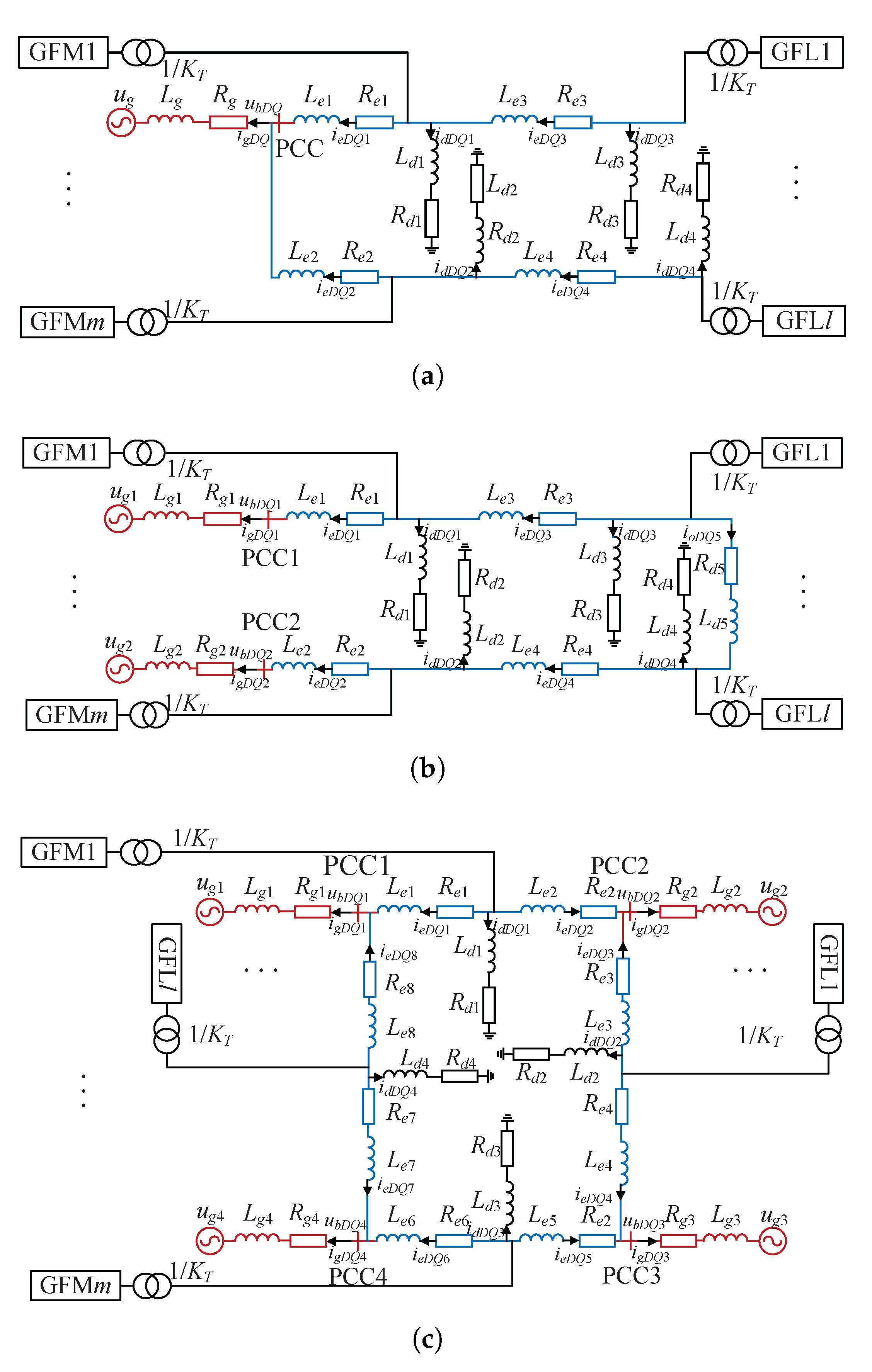
To validate the accuracy of the aforementioned theoretical analysis, the simulation models of the T1-, T2-, and T3-type grids are developed as illustrated in Figure 4 using Matlab/Simulink. This paper conducts research on two GFM inverters and two GFL inverters. Three grid topology structures adopt identical parameter sets as specified in

Table 1. System parameters.

Parameter	Value	Parameter	Value	Parameter	Value
$S_{\mathrm{B}}/\mathrm{kVA}$	5000	$L_{f\mathrm{l}1,2}/\mathrm{mH}$	0.0303	$L_{f\mathrm{m}1,2}/\mathrm{mH}$	0.4546
$U_{\mathrm{B}}/\mathrm{V}$	690	$R_{f\mathrm{l}1,2}/\Omega$	0.0004	$R_{f\mathrm{m}1,2}/\Omega$	0.0004
$U_{g\mathrm{B}}/\mathrm{V}$	10,500	$C_{f\mathrm{l}1,2}/\mathrm{F}$	0.0017	$C_{f\mathrm{m}1,2}/\mathrm{F}$	0.0017
$U_{cd}/\mathrm{V}$	1100	$k_{p\mathrm{pll}1,2}$	0.14	$D_{\mathrm{m}1,2}$	15
$U_g/\mathrm{V}$	10,500	$k_{i\mathrm{pll}1,2}$	3.08	$J_{\mathrm{m}1,2}$	0.1
$R_g/\Omega$	1.1025	$k_{pi\mathrm{l}1,2}$	0.8	$m_{\mathrm{m}1,2}$	20
$L_g/\mathrm{H}$	0.0234	$k_{ii\mathrm{l}1,2}$	5	$k_{pi\mathrm{m}1,2}$	0.8
$P_{d1,2}/\mathrm{kW}$	200	$k_{pp\mathrm{l}1,2}$	2	$k_{ii\mathrm{m}1,2}$	5
$P_{d3,4}/\mathrm{kW}$	100	$k_{ip\mathrm{l}1,2}$	50	$k_{pu\mathrm{m}1,2}$	5
$Q_{d1}/\mathrm{kVar}$	10	$R_e/\Omega$	0.0350	$k_{iu\mathrm{m}1,2}$	100
$Q_{d2,3,4}/\mathrm{kVar}$	40	$L_e/\mathrm{mH}$	0.1725	$K_T$	15.22

, where $S_{\mathrm{B}}$ denotes the base power of the system, $U_{\mathrm{B}}$ and $U_{g\mathrm{B}}$ represent the base voltages of the inverter and the grid, respectively. To simplify the model, the DC-side dynamics of the inverters are neglected and replaced by a constant voltage source $U_{cd}=1100$ V, producing an AC-side output voltage of 690 V. The grid voltage is set to 10,500 V, resulting in a transformer ratio $K_T$ = 10,500/690. The load connection powers are denoted as $P_d$ and $Q_d$.

4.1. Numerical Examples

The subsequent analysis will elucidate the state-space modeling process referenced above by employing the T1-type grid topology structure illustrated in Figure 4a with two GFM inverters and two GFL inverters. The detailed procedural steps are as follows:

• GFM inverter state space model. The linearized state-space equations for each GFM inverter are formulated according to Equations (1)–(3). A full-order state matrix Equation (4) ${\mathit{x}}_{\mathrm{m}1}\in {\mathbb{R}}^{10\times 1}$ and ${\mathit{x}}_{\mathrm{m}2}\in {\mathbb{R}}^{11\times 1}$ incorporating all GFM inverter state variables can be constructed.
• GFL inverter state space model. The linearized state-space equations for each GFL inverter are derived following Equations (5)–(7). A full-order state matrix Equation (8) ${\mathit{x}}_{\mathrm{l}1,2}\in {\mathbb{R}}^{12\times 1}$ incorporating all GFL inverter state variables can be constructed.
• Grid topology structure state space model. Based on the T1-type grid shown in Figure 4a, Equations (9) and (11) are derived to establish linearized state-space equations for each transmission line. This enables the construction of a full-order state matrix Equation (17) ${\mathit{x}}_e\in {\mathbb{R}}^{8\times 1}$, ${\mathit{x}}_d\in {\mathbb{R}}^{8\times 1}$ and ${\mathit{x}}_g\in {\mathbb{R}}^{3\times 1}$ that contains the dynamic characteristics of lines $L_e$, $L_d$, and $L_g$.
• Eliminate non-state variables. The transformation matrix ${\mathit{T}}_D$ defined in Equation (12) is applied by substituting ${\mathit{i}}_{odq}={\mathit{T}}_D{\mathit{i}}_{oDQ}$ and ${\mathit{u}}_{oDQ}={\mathit{T}}_D^{-1}{\mathit{u}}_{odq}$ into Equations (3) and (11), thereby replacing ${\mathit{i}}_{odq}$ and ${\mathit{u}}_{oDQ}$ with ${\mathit{i}}_{oDQ}$ and ${\mathit{u}}_{odq}$ through axis transformation. Following the T1-type grid topology in Figure 4a, Equation (14) is formulated and substituted into Equation (11) to replace ${\mathit{i}}_{oDQ}$ with branch currents ${\mathit{i}}_{eDQ}$ and ${\mathit{i}}_{dDQ}$. The PCC coupling Equation (16) corresponding to the T1-type grid is substituted into Equation (11) to eliminate the non-state variable ${\mathit{u}}_{bDQ}$. At this point, all non-state variables are replaced by state variables.
• System full-order state space variables. Consolidate and combine Equations (1)–(3), (5)–(7), (9) and (11) to compile all linearized state-space equations into the unified system model Equation (18). Simultaneously, combine state matrices Equations (4), (8) and (17) to derive the complete state vector ${\mathit{x}}_{\mathrm{s}1}=[{\mathit{x}}_{\mathrm{m}1},{\mathit{x}}_{\mathrm{m}2},{\mathit{x}}_{\mathrm{l}1},{\mathit{x}}_{\mathrm{l}2},{\mathit{x}}_e,{\mathit{x}}_d,{\mathit{x}}_g]\in {\mathbb{R}}^{64\times 1}$ encompassing all state variables. The specific expression of ${\mathit{x}}_{\mathrm{s}1}$ is shown in Equation (A1) of the Appendix B.
• System full-order state space model. Extract the coefficients of state variables from the aggregated state-space Equation (18) to construct the system state matrix ${\mathit{A}}_{\mathrm{s}1}\in {\mathbb{R}}^{64\times 64}$, explicitly formulated in Equation (19). By substituting the parameters in Table 1 into each element of the matrix ${\mathit{A}}_{\mathrm{s}1}$, the specific expression of ${\mathit{A}}_{\mathrm{s}1}$ can be obtained.
• Calculate eigenvalues and participation factors. The eigenvalues and participation factors of the state matrix ${\mathit{A}}_{\mathrm{s}1}$ are computed using MATLAB, yielding 64 eigenvalues corresponding to the total number of state variables ${\mathit{x}}_{\mathrm{s}1}$ and a participation factor matrix ${\mathbf{P}}_{\mathrm{s}1}$ that quantifies the contribution of each state variable to eigenvalues.
• Calculate eigenvalue variations. Selected participation factors from Equation (22), (24) and (26) are extracted. Incremental variations of $k_{p\mathrm{plll}1,2}$, $k_{i\mathrm{plll}1,2}$, $D_{\mathrm{m}1,2}$ and $Z_e$ are introduced into these equations to calculate three sets of eigenvalue variations $\Delta \lambda$. This enables the determination of the changing trend of the dominant eigenvalue.
• Calculate the oscillation frequency and damping ratio. The oscillation frequency f is derived from the imaginary parts of the dominant eigenvalues, while the damping ratio $\zeta$ is obtained from their real parts. State variables with participation factors below 0.1 are prioritized for analysis to identify dominant contributors to critical oscillation modes.
• Simulation verification. A Simulink model of the T1-type grid is implemented for validation. Simulations are performed using the parameters listed in Table 1 to generate system active power waveforms. The oscillation frequency and divergence/convergence characteristics of the waveforms are analyzed and compared with the calculated frequency f and damping ratio $\zeta$ from the previous step, thereby validating the accuracy of the state-space modeling approach.

The analysis process for T2- and T3-type grids is similar to that of T1-type. Their full-order state variables are as shown in Equations (A2) and (A3) in Appendix B.

4.2. Simulation Validation of Grid Topology Impact on GFL-Dominant Oscillation Modes

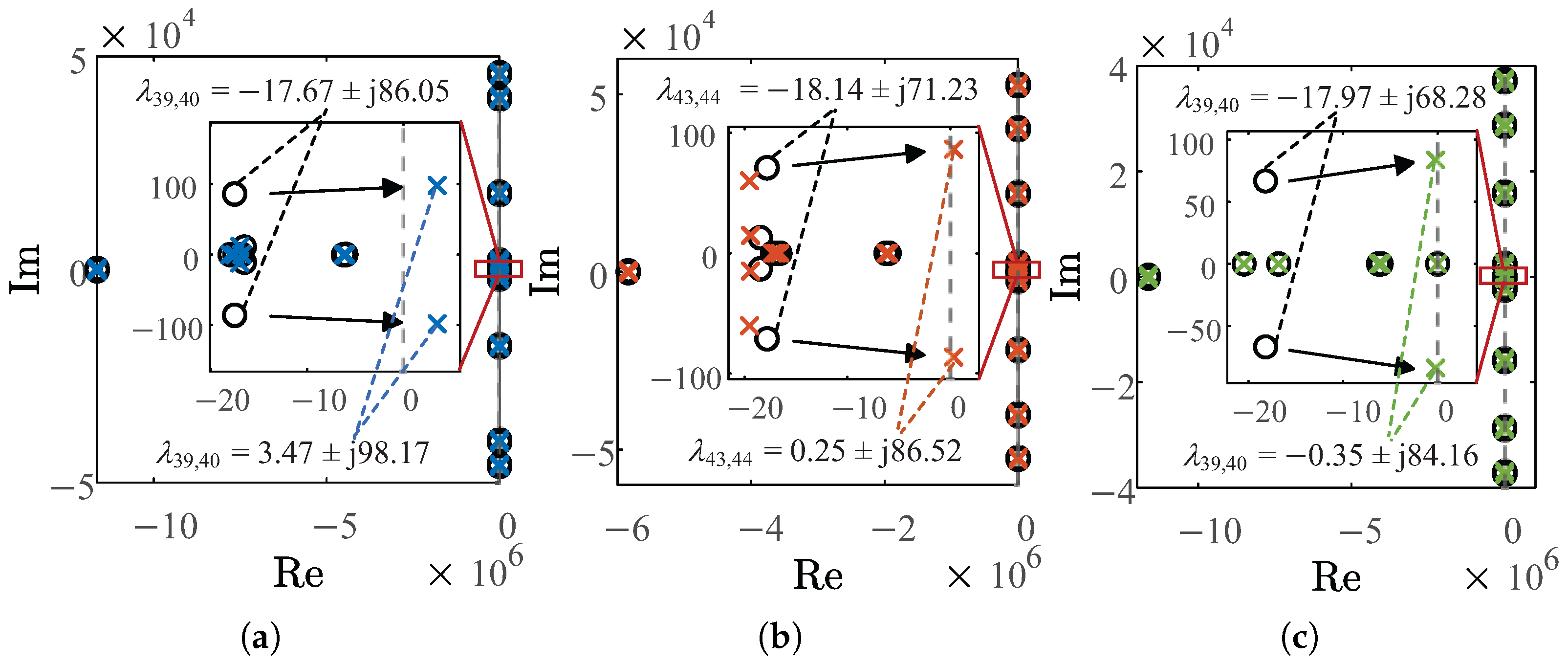
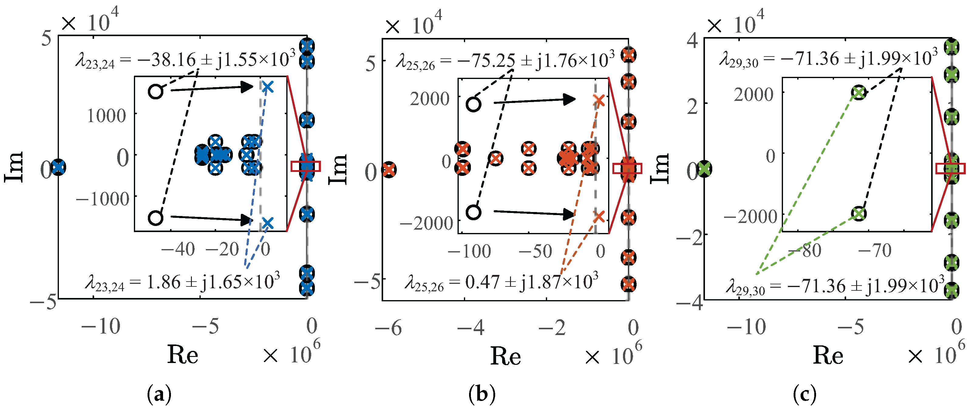
In order to analyze the impact of grid topology structure on the dominant oscillation modes of the GFL inverters, the dominant eigenvalues of the GFL inverters are first identified. Based on the initial parameters in Table 1, gradually increase $k_{p\mathrm{plll}1,2}$ and $k_{i\mathrm{plll}1,2}$, and observe that when $k_{p\mathrm{plll}1,2}=9$ and $k_{i\mathrm{plll}1,2}=1960$, the full-order eigenvalues of three grid topology structures are shown in Figure 5a–c. The eigenvalues dominated by GFL inverters in the T1-, T2-, and T3-type topology structures are ${\lambda }_{23,24}=-38.16\pm \mathrm{j}1.55\times {10}^3$, ${\lambda }_{25,26}=-75.25\pm \mathrm{j}1.76\times {10}^3$, and ${\lambda }_{29,30}=-71.36\pm \mathrm{j}1.99\times {10}^3$, respectively. Then, with increments $\Delta k_{p\mathrm{plll}1,2}=0.3$ and $\Delta k_{i\mathrm{plll}1,2}=60$, the increase in the dominant eigenvalues of three grid topology structures can be calculated using Equation (22), causing $\Delta {\lambda }_{23,24}=3.60\pm \mathrm{j}7.51$, $\Delta {\lambda }_{25,26}=6.60\pm \mathrm{j}8.32$, and $\Delta {\lambda }_{29,30}=0$, respectively. This demonstrates that increasing $k_{p\mathrm{plll}1,2}$ and $k_{i\mathrm{plll}1,2}$ shifts the eigenvalues of the system along the real axis toward the right half-plane (RHP), indicating reduced stability margins. Continue to increase $k_{p\mathrm{plll}1,2}=13.5$ and $k_{i\mathrm{plll}1,2}=3000$, and the full-order eigenvalues of three grid topology structures are shown in Figure 5. Under these parameters, ${\lambda }_{23,24}=1.86\pm \mathrm{j}1.65\times {10}^3$, ${\lambda }_{25,26}=0.47\pm \mathrm{j}1.87\times {10}^3$, and ${\lambda }_{29,30}=-71.36\pm \mathrm{j}1.99\times {10}^3$, respectively, are listed in

Table 2. The dominant eigenvalue of the GFL inverters when $k_{p\mathrm{plll}1,2}=13.5$ and $k_{i\mathrm{plll}1,2}=3000$.

Grid Type	$\mathit{\lambda }$	f (Hz)	$\mathit{\zeta }$ (%)	Participation Factor (>0.1)
T1	${\lambda }_{23,24}=1.86$ $\pm \mathrm{j}1.65\times {10}^3$	262.3	−0.0020	${\delta }_{\mathrm{l}1,\mathrm{l}2}=0.1790$ $i_{gq}=0.2017$
T2	${\lambda }_{25,26}=0.47$ $\pm \mathrm{j}1.87\times {10}^3$	298.2	−0.0003	${\delta }_{\mathrm{l}1,\mathrm{l}2}=0.1774$ $i_{gq1,2}=0.1455$
T3	${\lambda }_{29,30}=-71.36$ $\pm \mathrm{j}1.99\times {10}^3$	316.7	0.0358	${\delta }_{\mathrm{l}1,\mathrm{l}2}=0.2338$ $i_{gq1,2,3,4}=0.2196$

.

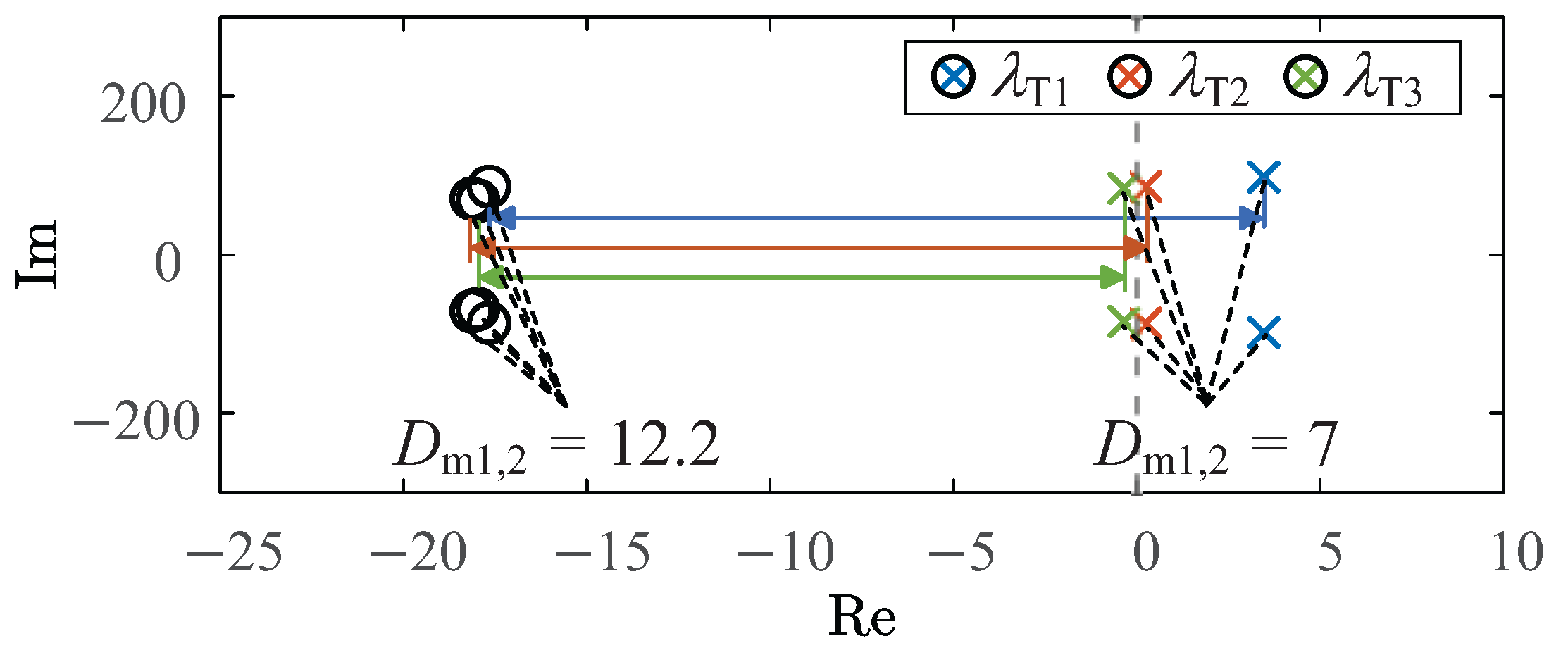
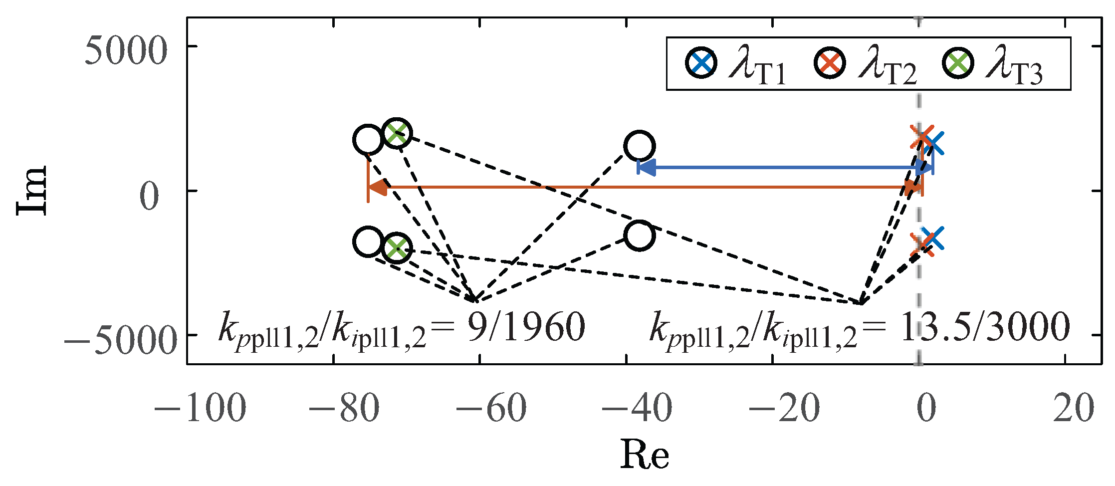
As evidenced in Figure 5, it can be observed that a pair of dominant eigenvalues move to the RHP under three different grid topology structures, whereas other system eigenvalues remain stationary. This observation confirms that the stability characteristics of GFL inverters under different grid topology structures can be effectively characterized by these migrating eigenvalue pairs. To enable focused analysis, we have reconstructed the migration trajectories of these three critical eigenvalue pairs from Figure 5 into the comparative plot shown in Figure 6. The distance between points ‘o’ and ‘x’ in the Figure 6 represents the stability region of eigenvalues when GFL inverters undergo identical parameter variations under three grid topology structures.It can be observed that with increasing proportional and integral coefficients of the PLL, the eigenvalues of both grid topology structures are shifted right along the real axis, consistent with the eigenvalue variation analysis $\Delta \lambda$ presented earlier. Observing Figure 6, it can be seen that, under the same initial parameters $k_{p\mathrm{plll}1,2}=9$ and $k_{i\mathrm{plll}1,2}=1960$, the eigenvalues of T1-type grid topology structure are the farthest to the right. Under the same parameter variations, the real parts of the eigenvalues in the T1-type grid are the first to cross the imaginary axis, followed by those in the T2-type grid. By observing the eigenvalue trajectories of three grid topology structures under the same parameter variations, it can be seen that the feasible parameter domain of the T1-type grid is smaller than that of the T2-type grid. For the T3-type grid, its eigenvalues remain invariant under parameter variations. This demonstrates that GFL inverters in T3-type grid topology structure exhibit high stability and robustness. That is, GFL inverters possess a larger feasible region under strong grid conditions.

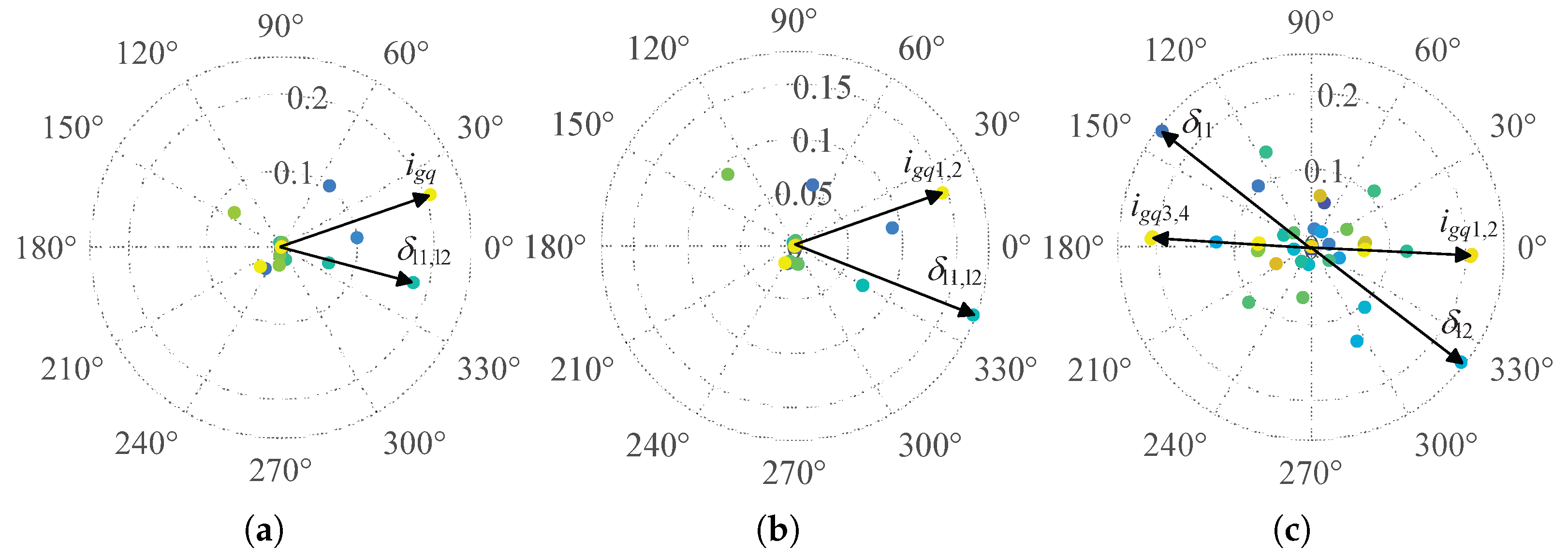
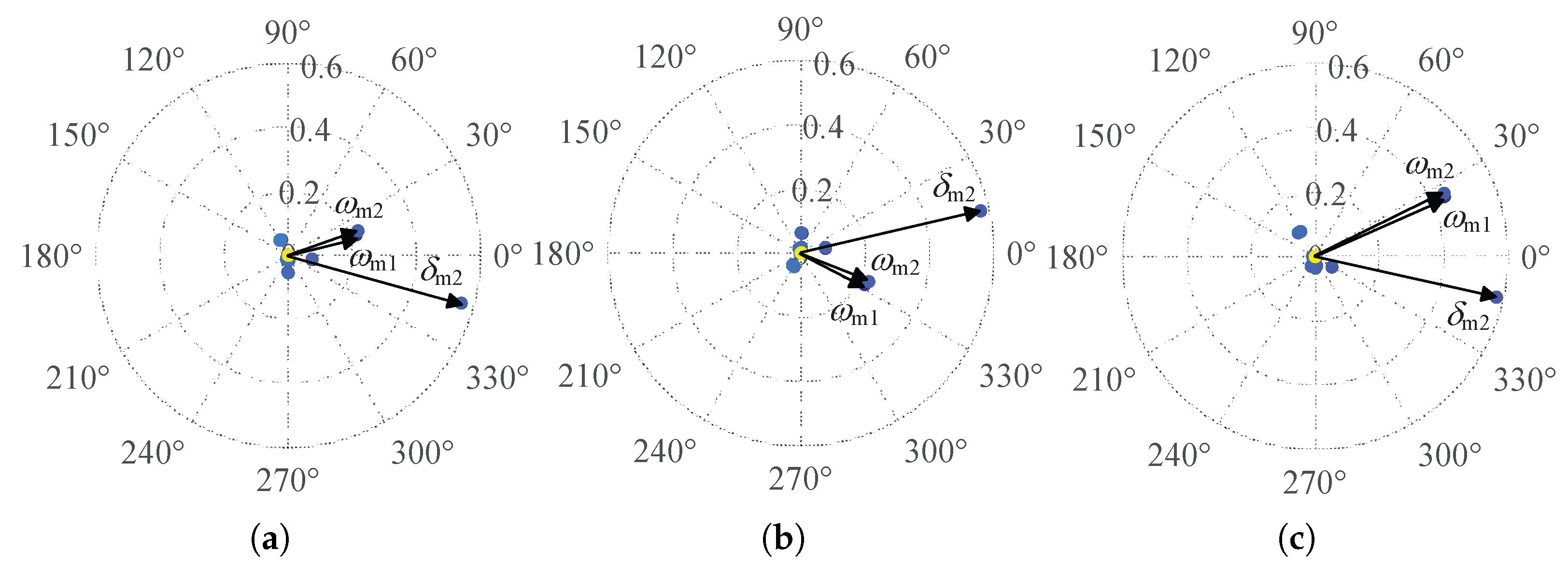
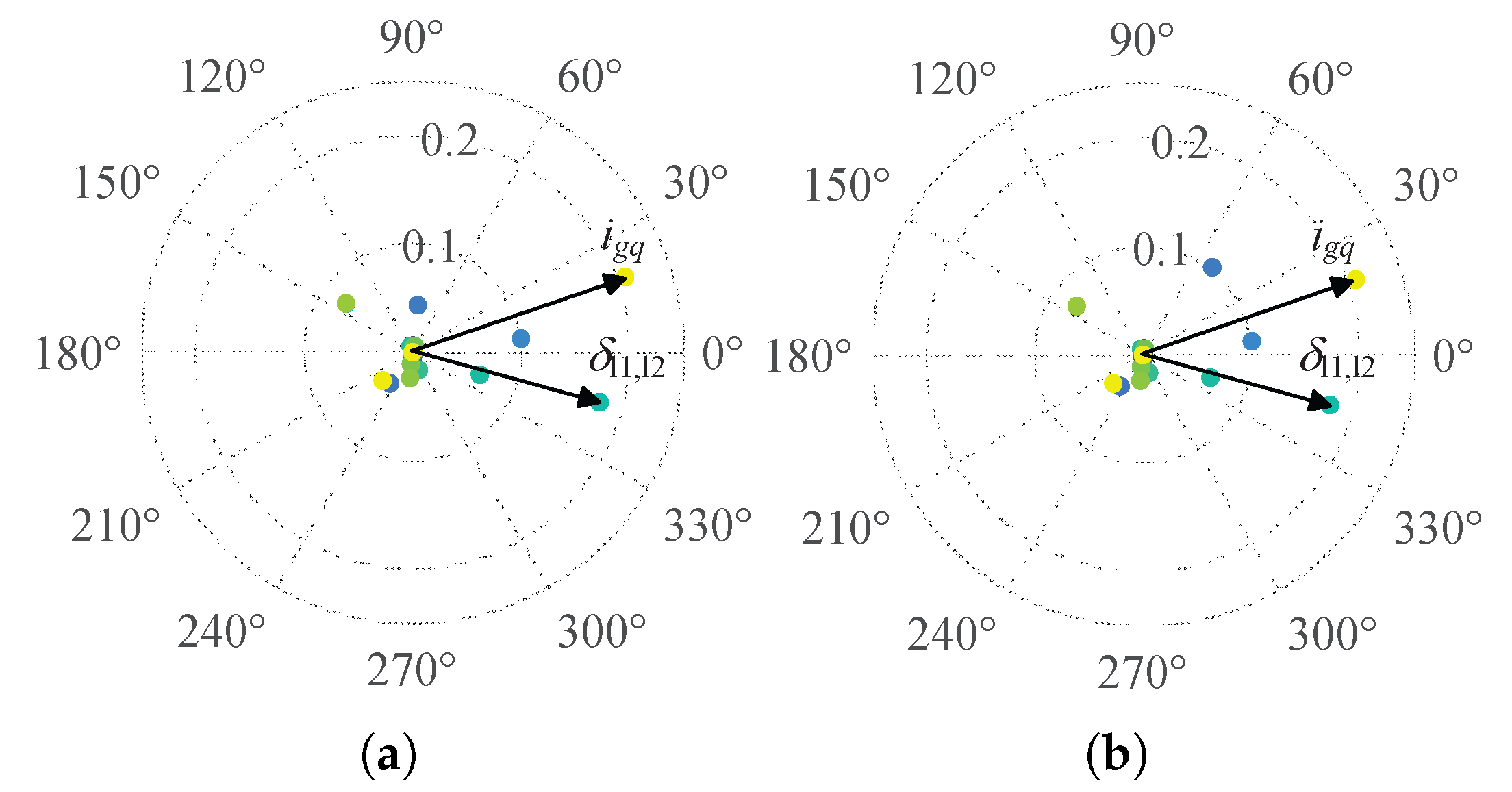
Under the operating conditions of $k_{p\mathrm{plll}1,2}=13.5$ and $k_{i\mathrm{plll}1,2}=3000$, the small signal analysis of eigenvalues is presented in Table 2. The whole participation factors of the three pairs of eigenvalues are calculated and represented by colored dots as shown in Figure 7, respectively. In the participation factor graph, those greater than 0.1 are considered key state variables, which have a significant degree of participation in the eigenvalues and are indicated by arrows in Figure 7. In the T1-type grid, the highest participation factor is observed in $i_{gq}$, followed by ${\delta }_{\mathrm{l}1,\mathrm{l}2}$. For the T2-type grid, the participation factors of both $i_{gq1,2}$ and ${\delta }_{\mathrm{l}1,\mathrm{l}2}$ are reduced compared to the T1-type grid. According to the definition of the state-space model, ${\delta }_{\mathrm{l}1,\mathrm{l}2}$ represents the interaction between the GFL and the GFM1 inverter. $i_{gq}$ represents the influence of the q-axis component of the current of the grid on the GFL inverters, which partially quantifies the impact of the grid on the dynamics of the GFL inverters. As indicated by the participation factor results, it can be seen that the influence of the grid on the GFL inverters is reduced in the T2-type grid, and the interaction between the GFL and the GFM1 inverter is also weakened. For the T3-type grid, the participation factors of both $i_{gq1,2,3,4}$ and ${\delta }_{\mathrm{l}1,\mathrm{l}2}$ increase compared to the T1- and T2-type grids. This is attributed to the closer proximity of the GFL inverters to the infinite grid in the T3-type grid topology structure.

Meanwhile, a small signal analysis is conducted on three eigenvalue pairs corresponding to $k_{p\mathrm{plll}1,2}=13.5$ and $k_{i\mathrm{plll}1,2}=3000$, and the results are presented in Table 2. A comparison of the oscillation frequencies f reveals that the T3-type grid exhibits a higher frequency than the T2- and T1-type grid. Furthermore, the damping ratios $\zeta$ for the T1, T2 and T3-type grids are measured as $-0.0020\%$ and $-0.0003\%$ respectively, signifying the presence of time-divergent oscillations in both systems. However, the T2-type grid demonstrates a relatively larger damping ratio, resulting in a slower rate of oscillatory divergence. The damping ratio of the T3-type grid is greater than zero, which indicates that no oscillations in T3-type grid.

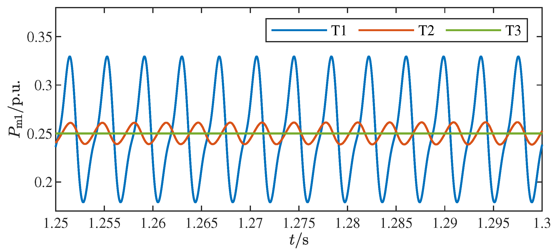
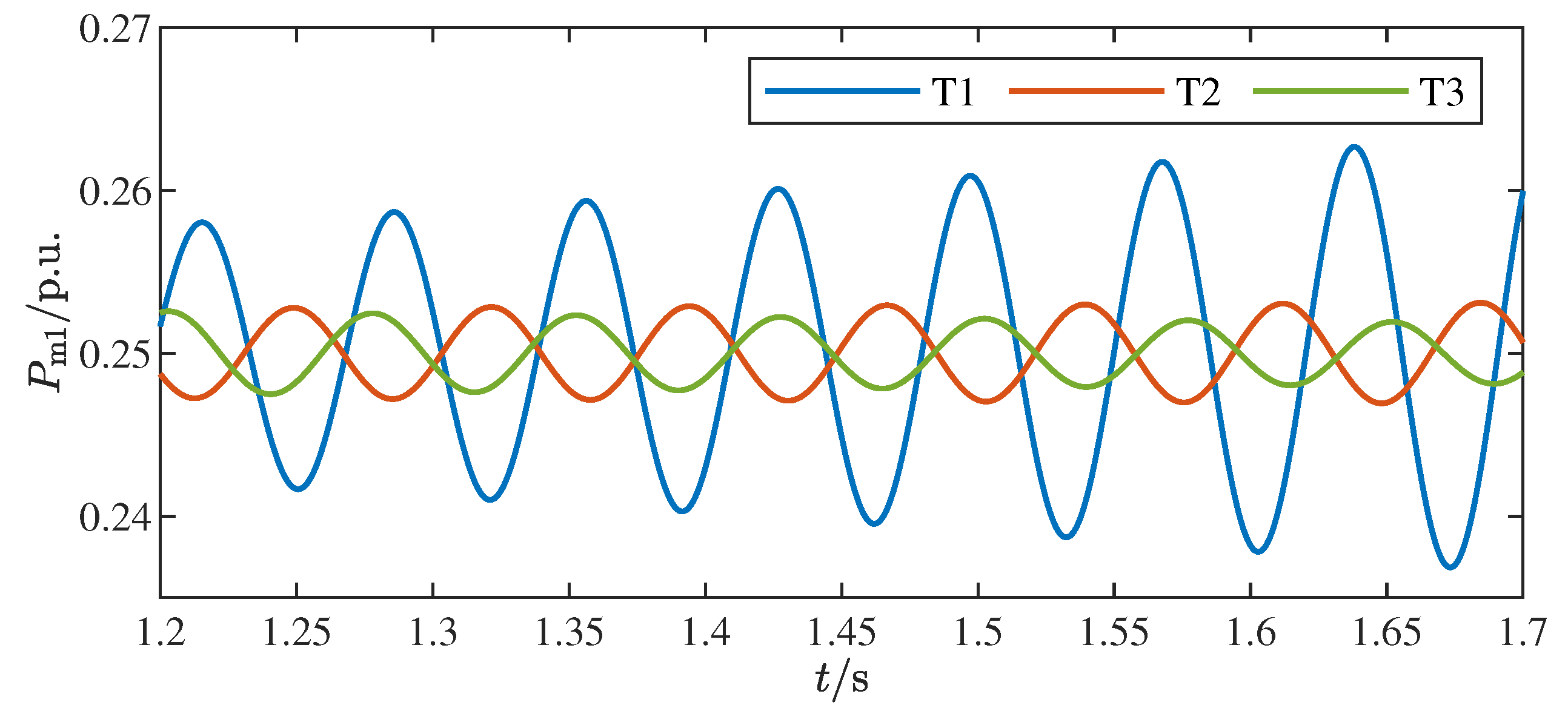
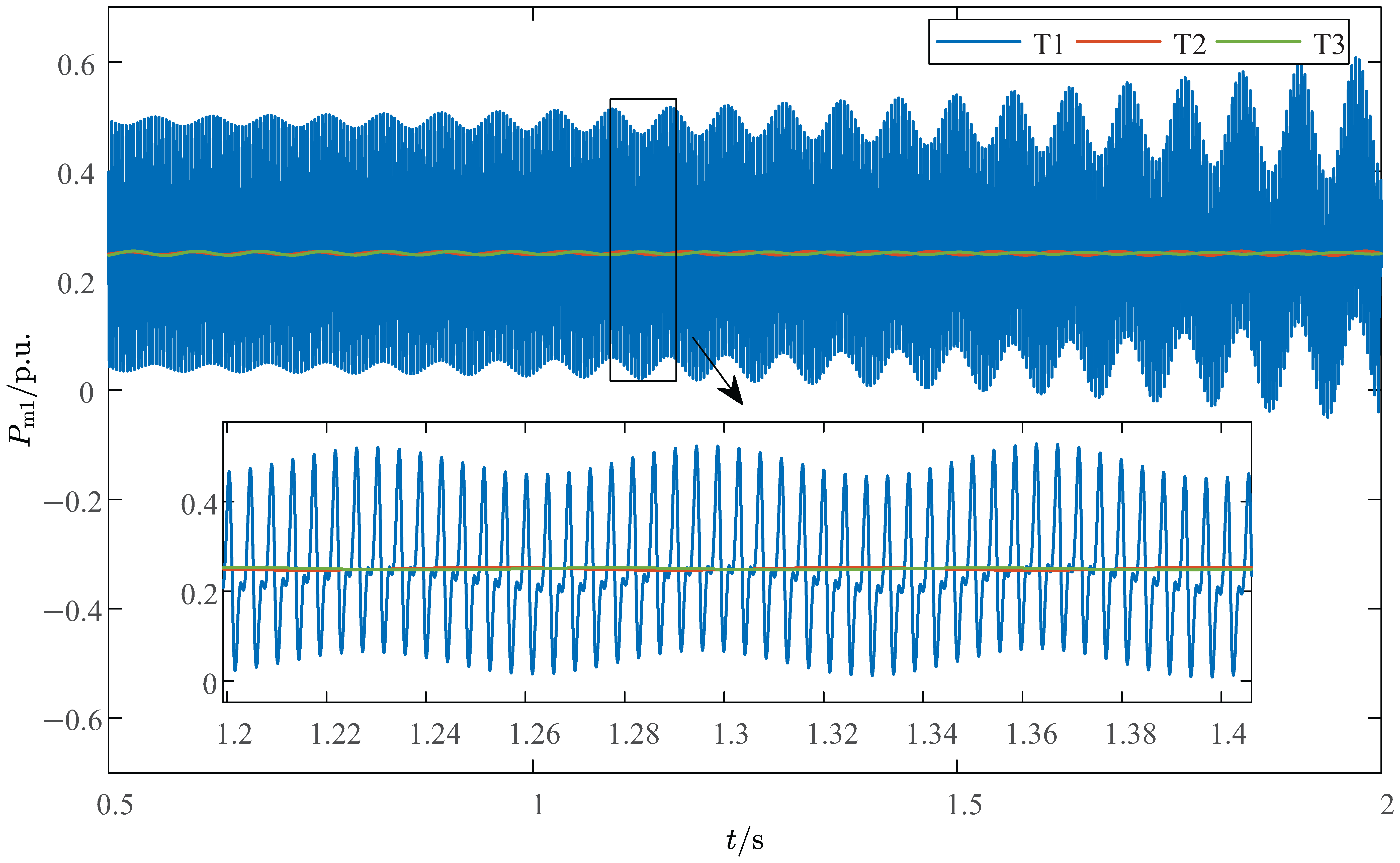
To further validate the stability of grid topology structures, Figure 8 presents the simulation results in the time domain of the normalized active power $P_{\mathrm{m}1}$ of the GFM1 inverter when $k_{p\mathrm{plll}1,2}=13.5$ and $k_{i\mathrm{plll}1,2}=3000$. In order to more intuitively show the differences among the three sets of curves, the waveform graph from 1.25 to 1.3 s is selected for analysis. It can be distinctly observed that as grid topology structure is transitioned from Type T1 to Type T3, the stability of the GFL inverter is progressively enhanced, with oscillatory behavior becoming increasingly suppressed. In particular, in the T3-type grid configuration, no oscillations are observed throughout the system. This confirms that the grid has a high degree of participation in the oscillation mode of the GFL inverter, which aligns with the theoretical analysis presented earlier.

Through fast Fourier transform (FFT) analysis of the simulation waveforms, it can be obtained that the oscillation frequencies of the blue and orange curves are 261 and 301 Hz, respectively, demonstrating a sequential frequency escalation. The results in the time domain are consistent with the analysis results of f in Table 2. In Figure 8, the blue and orange curves have oscillations that diverge over time, whereas the green curve does not. This behavior indicates that the damping ratios $\zeta$ of the T1 and T2-type grids are negative, while the T3-type grid achieves a positive damping ratio. The results in the time domain are consistent with the analysis results of $\zeta$ in Table 2.

In conclusion, the grid has a high degree of participation in the dominant oscillation mode of the GFL inverters. Under identical parameter sets, the damping ratios $\zeta$ of T1-, T2-, and T3-type grids increase successively. With identical parameter variations, the T3-type grid is less prone to instability than the T2-type grid, and the T2-type grid exhibits higher stability than the T1-type grid. As grid topology structure is transitioned from T1- to T3-type, the stability of the GFL inverters and the robustness of the system gradually improve. Consequently, GFL inverters are optimally recommended for integration into robust grids such as the T2- and T3-type grid.

4.3. Simulation Validation of Grid Topology Impact on GFM Inverters Dominant Oscillation Modes

Similar to the previous subsection, based on the initial parameters in Table 1, gradually decrease $D_{\mathrm{m}1,2}$, and observe that when $D_{\mathrm{m}1,2}=12.2$, the full-order eigenvalues are shown as in Figure 9a–c. The eigenvalues dominated by GFM inverters in the three type topology structures are ${\lambda }_{39,40}=-17.67\pm \mathrm{j}86.05$, ${\lambda }_{43,44}=-18.14\pm \mathrm{j}71.23$, and ${\lambda }_{52,53}=-17.97\pm \mathrm{j}68.28$, respectively. Then, with reduction $\Delta D_{\mathrm{m}1,2}=0.3$, the dominant increase in the eigenvalues can be calculated using Equation (24). The $\Delta {\lambda }_{39,40}=1.12\pm \mathrm{j}1.02$, $\Delta {\lambda }_{43,44}=0.79\pm \mathrm{j}1.22$, and $\Delta {\lambda }_{52,53}=0.71\pm \mathrm{j}1.25$, respectively. This demonstrates that decreasing $D_{\mathrm{m}1,2}$ shifts the eigenvalues of the system along the real axis toward the RHP, indicating reduced stability margins. Continuing to decrease $D_{\mathrm{m}1,2}=7$, the full-order eigenvalues are shown in Figure 9. Under these parameters, ${\lambda }_{39,40}=3.47\pm \mathrm{j}98.17$, ${\lambda }_{43,44}=0.25\pm \mathrm{j}86.52$, and ${\lambda }_{52,53}=-0.35\pm \mathrm{j}84.16$, respectively.

Similar to the previous analysis, the main eigenvalues of the GFM inverters extracted from Figure 9 are shown in Figure 10. The distance between points ‘o’ and ‘x’ in the Figure 10 represents the stability region of eigenvalues when GFM inverters undergo identical parameter variations under three grid topology structures. It can be observed that with the decreasing damping coefficient $\Delta D_{\mathrm{m}1,2}$, the eigenvalues of both grid topology structures are shifted RHP along the real axis, consistent with the eigenvalue variation analysis $\Delta \lambda$ presented earlier. Observing Figure 10, it can be seen that the variation pattern of the eigenvalues is similar to that of the GFL inverters. Notably, by observing the eigenvalue trajectories of three grid topology structures under the same parameter variations, it can be seen that the feasible parameter domain of T1-type grid is bigger than that of T2-type grid, and T3-type grid is minimum. This result is contrary to that of GFL inverters. This demonstrates that GFM inverters possess a smaller parameter feasible region under strong grid conditions.

Under the operating conditions of $D_{\mathrm{m}1,2}=7$, the small signal analysis of the eigenvalues is presented in

Table 3. The dominant eigenvalue of the GFM inverters when $D_{\mathrm{m}1,2}=7$.

Type	$\mathit{\lambda }$	f (Hz)	$\mathit{\zeta }$ (%)	Participation Factor (>0.1)
T1	${\lambda }_{39,40}=3.47$ $\pm \mathrm{j}98.17$	$15.6$	$-0.0353$	${\delta }_{\mathrm{m}2}=0.5597$ ${\omega }_{\mathrm{m}1}=0.2207$ ${\omega }_{\mathrm{m}2}=0.2304$
T2	${\lambda }_{43,44}=0.25$ $\pm \mathrm{j}86.52$	$13.7$	$-0.0029$	${\delta }_{\mathrm{m}2}=0.5732$ ${\omega }_{\mathrm{m}1}=0.2202$ ${\omega }_{\mathrm{m}2}=0.2279$
T3	${\lambda }_{52,53}=-0.35$ $\pm \mathrm{j}84.16$	$13.4$	$0.0041$	${\delta }_{\mathrm{m}2}=0.5771$ ${\omega }_{\mathrm{m}1}=0.4376$ ${\omega }_{\mathrm{m}2}=0.4467$

. The whole participation factors of the three pairs of eigenvalues are calculated and represented by colored dots as shown in Figure 11, respectively. Across three grid topology structures, significant participation factors are observed in ${\delta }_{\mathrm{m}2}$, ${\omega }_{\mathrm{m}1}$, and ${\omega }_{\mathrm{m}2}$. The participation levels of other state variables remain below 0.1, indicating a negligible influence on the eigenvalues. The state variable $i_{gq}$ related to the power grid is consistently found to be minimal, indicating that the power grid has a minor influence on the GFM inverters. ${\delta }_{\mathrm{m}2}$ characterizes the interaction among the GFM inverters. From T1- to T3-type, the degree of participation has increased slightly. This indicates that the interaction between the GFM inverters is strengthened under stronger grid conditions. ${\omega }_{\mathrm{m}1}$ and ${\omega }_{\mathrm{m}2}$ represent the frequency characteristics of the synchronous loops of the GFM1 and GFM2 inverters, respectively, which exhibit nearly identical participation levels on the T1 and T2-type grids. However, a substantial increase in their participation factors is observed in the T3-type grid, demonstrating that the stability of GFM inverters under a strong grid condition is more susceptible to the influence of their synchronization loop control capabilities.

Meanwhile, a small signal analysis is conducted on three eigenvalue pairs corresponding to $D_{\mathrm{m}1,2}=7$, and the results are presented in Table 3. A comparison of the oscillation frequencies f reveals a progressive decline from T1 to T3-type. Furthermore, the damping ratios $\zeta$ for T1 and T2-type grids are measured as $-0.0353\%$ and $-0.0029\%$ respectively, signifying time-divergent oscillations in both configurations. In particular, the T2-type grid exhibits a relatively higher damping ratio, resulting in slower oscillatory divergence. In contrast, the T3-type grid achieves a positive damping ratio $0.0041\%$, indicative of time-convergent oscillations.

Figure 12 presents the simulation results in the time domain of the normalized active power $P_{\mathrm{m}1}$ of the GFM1 inverter when $D_{\mathrm{m}1,2}=7$. It is evident that as grid topology structure is transitioned from T1 to T3, the GFM inverters become increasingly stabilized, with oscillations gradually attenuated. However, the synchronization control of the GFM inverter still causes oscillations despite the grid intensity being stronger. It indicates that increasing the intensity of the grid can only partially improve the stability of GFM inverters, while the synchronization control capability of the inverters plays a more dominant role. It is different from the research results of the GFL inverters.

Through FFT analysis of the simulation waveforms, it can be obtained that the oscillation frequencies of the blue and orange curves are 15 Hz and 14 Hz, respectively, and the green curve is 13.6 Hz. The oscillation frequencies decrease subsequently. The results in the time domain are consistent with the analysis results of f in Table 3. The blue and orange curves exhibit time-divergent oscillations, whereas the green curve shows time-convergent oscillation. This confirms that the damping ratios are negative for T1 and T2-type grids, but positive for T3-type. The results in the time domain are consistent with the analysis results of $\zeta$ in Table 3.

In conclusion, under identical parameter sets, the damping ratios $\zeta$ of the T1-, T2-, and T3-type grids increase successively. As grid topology structure is transitioned from T1- to T3-type, the stability of GFM inverters gradually improves, although the enhancement remains limited. With identical parameter variations, the robustness of the system gradually reduces. The stability of the GFM inverter is more critically governed by its intrinsic synchronization control capability. Consequently, optimizing the synchronization loop dynamics will lead to greater stability improvements in GFM inverters.

4.4. Stability Analysis and Simulation Verification of Different Grid Topology Structures Under Simultaneous Parameter Variations in GFM and GFL Inverters

In this subsection, we discuss the stability characteristic of the system under diverse grid topologies when the parameters of both GFL and GFM inverters change simultaneously. Initially, through a comparison between Equations (22) and (24), it becomes evident that the variation of the system’s eigenvalues depends on the participation factors associated with $k_{p\mathrm{plll}1,2}$, $k_{i\mathrm{plll}1,2}$, and $D_{\mathrm{m}1,2}$. A comparison of these two equations reveals that the participation factors related to $k_{p\mathrm{plll}1,2}$ and $k_{i\mathrm{plll}1,2}$ are entirely independent of those related to $D_{\mathrm{m}1,2}$. This indicates that when $k_{p\mathrm{plll}1,2}$, $k_{i\mathrm{plll}1,2}$, and $D_{\mathrm{m}1,2}$ undergo simultaneous changes, within the system’s full-order eigenvalues, there will be two pairs of completely independent eigenvalues that change correspondingly. Herein, we adopt the same parameter variations as previously described: $k_{p\mathrm{plll}1,2}$ and $k_{i\mathrm{plll}1,2}$ are adjusted from 0.14 and 3.08 to 13.5 and 3000, while $D_{\mathrm{m}1,2}$ is modified from 15 to 7. The eigenvalues that change in the system under three grid topology structures when $k_{p\mathrm{plll}1,2}=13.5$, $k_{i\mathrm{plll}1,2}=3000$ and $D_{\mathrm{m}1,2}=7$ are presented in

Table 4. The dominant eigenvalue of the GFL and GFM inverters when $k_{p\mathrm{plll}1,2}=13.5$, $k_{i\mathrm{plll}1,2}=3000$ and $D_{\mathrm{m}1,2}=7$.

Grid Type	$\mathit{\lambda }$	f (Hz)	$\mathit{\zeta }$ (%)	Participation Factor (>0.1)
T1	${\lambda }_{23,24}=1.85$ $\pm \mathrm{j}1.64\times {10}^3$	262.3	−0.0020	${\delta }_{\mathrm{l}1,\mathrm{l}2}=0.1790$ $i_{gq}=0.2071$
	${\lambda }_{43,44}=4.79$ $\pm \mathrm{j}98.59$	15.7	−0.0485	${\delta }_{\mathrm{m}2}=0.5523$ ${\omega }_{\mathrm{m}1}=0.2200$ ${\omega }_{\mathrm{m}2}=0.2297$
T2	${\lambda }_{25,26}=0.47$ $\pm \mathrm{j}1.87\times {10}^3$	298.9	−0.0018	${\delta }_{\mathrm{l}1,\mathrm{l}2}=0.1774$ $i_{gq1,2}=0.1455$
	${\lambda }_{47,48}=1.51$ $\pm \mathrm{j}87.07$	13.8	−0.0174	${\delta }_{\mathrm{m}2}=0.5651$ ${\omega }_{\mathrm{m}1}=0.2202$ ${\omega }_{\mathrm{m}2}=0.2280$
T3	${\lambda }_{29,30}=-71.36$ $\pm \mathrm{j}1.99\times {10}^3$	316.5	0.0359	${\delta }_{\mathrm{l}1,\mathrm{l}2}=0.2443$ $i_{gq1,2,3,4}=0.2076$
	${\lambda }_{48,49}=0.90$ $\pm \mathrm{j}84.75$	13.5	−0.0106	${\delta }_{\mathrm{m}2}=0.5771$ ${\omega }_{\mathrm{m}1}=0.4376$ ${\omega }_{\mathrm{m}2}=0.4467$

.

It can be seen from the Table 4 that the systems under three grid topologies all possess two pairs of eigenvalues with positive real parts. Initially, a comparison is made between the eigenvalues ${\lambda }_{23,24}$, ${\lambda }_{25,26}$, and ${\lambda }_{29,30}$ presented in Table 4 and those in Table 2. It is obvious that these eigenvalues are dominated by the GFL inverter. When the parameters of both the GFL and GFM inverters undergo simultaneous changes, the dominant eigenvalues of the GFL exhibit negligible differences in oscillation frequency f, damping coefficient $\zeta$, and participation factors when compared to those obtained in Table 2. Meanwhile, through a comparison of the eigenvalues of ${\lambda }_{43,44}$, ${\lambda }_{47,48}$, and ${\lambda }_{48,49}$ presented in Table 4 with those governed by the GFM inverter in Table 3, the identical conclusion can be reached. Thus, the example data effectively corroborates the analysis results of Equations (22) and (24) in the foregoing text. Specifically, the oscillations governed by the GFL and GFM inverters are entirely independent.

To better validate the above results, Figure 13 shows the time-domain simulation results of the active power $P_{\mathrm{m}1}$ under the conditions $k_{p\mathrm{plll}1,2}=13.5$, $k_{i\mathrm{plll}1,2}=3000$ and $D_{\mathrm{m}1,2}=7$. FFT analysis of the three waveforms in Figure 13 reveals that the T1-type grid waveform contains oscillation frequencies of 261 Hz and 15 Hz, indicating a superposition of these two frequencies. The T2-type grid waveform exhibits oscillation frequencies of 303 Hz and 14 Hz. However, since the real parts of ${\lambda }_{23,24}$ in the T2-type grid system are very small, the 303 Hz oscillation component is negligible, and the waveform is predominantly governed by the 14 Hz oscillation. In the T3-type grid, the real parts of ${\lambda }_{29,30}$ are negative, meaning the potential oscillation modes are not excited. Consequently, the T3-type grid waveform only contains a decaying 13 Hz oscillation frequency over time.

In summary, the oscillations dominated by GFL and GFM inverters are entirely independent. The separate analysis of dominant oscillation modes in GFL and GFM inverters is justified in the previous analysis.

4.5. Stability Analysis of GFL and GFM Inverters in Hybrid Grid Topology Structures

In this section, we analyze the stability of GFL and GFM inverters in hybrid grid topology structures. First, traditional power grids are predominantly radial in structure. To improve power supply flexibility and enable rapid post-fault recovery, single-ended radial grids can be modified to form ring-type grids. As grid scales continue to expand, ensuring interconnection and mutual support between multi-regional grids requires interconnecting multiple ring-type grids, ultimately forming meshed-type grids.

In Figure 4, all infinite power grid supplies are denoted by red segments, while all connection lines are indicated by blue segments. As shown in Figure 4a,b, the T2-type grid can be derived by directly interconnecting the endpoints of two T1-type grids from Figure 4a and simplifying the intermediate connections. Comparing Figure 4b with Figure 4c, each pair of adjacent infinite grids in the T3-type grid and their connecting lines form a simplified T2-type grid. Therefore, the T2-type grid represents a hybrid connection of T1-type grids. The T3-type grid can be regarded as a hybrid connection of T2-type and T1-type grids. Based on the above analysis, the following conclusions can be drawn: In the T3-type hybrid grid topology, GFL inverters exhibit superior stability compared to T2-type and T1-type grids. GFM inverters show moderate stability improvement but are more sensitive to their own synchronization control loops.

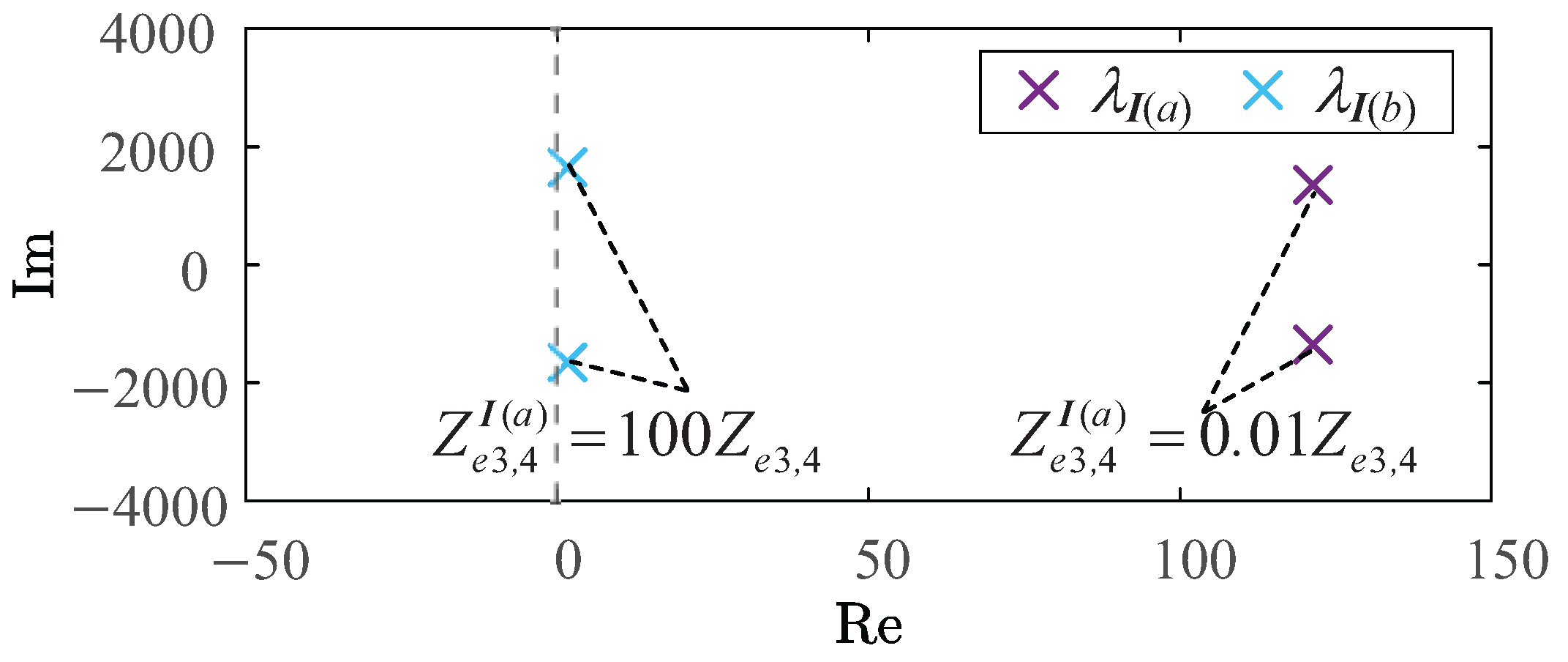
4.6. Simulation Validation of Grid Impedance Impact on Inverter Dominant Oscillatory Modes

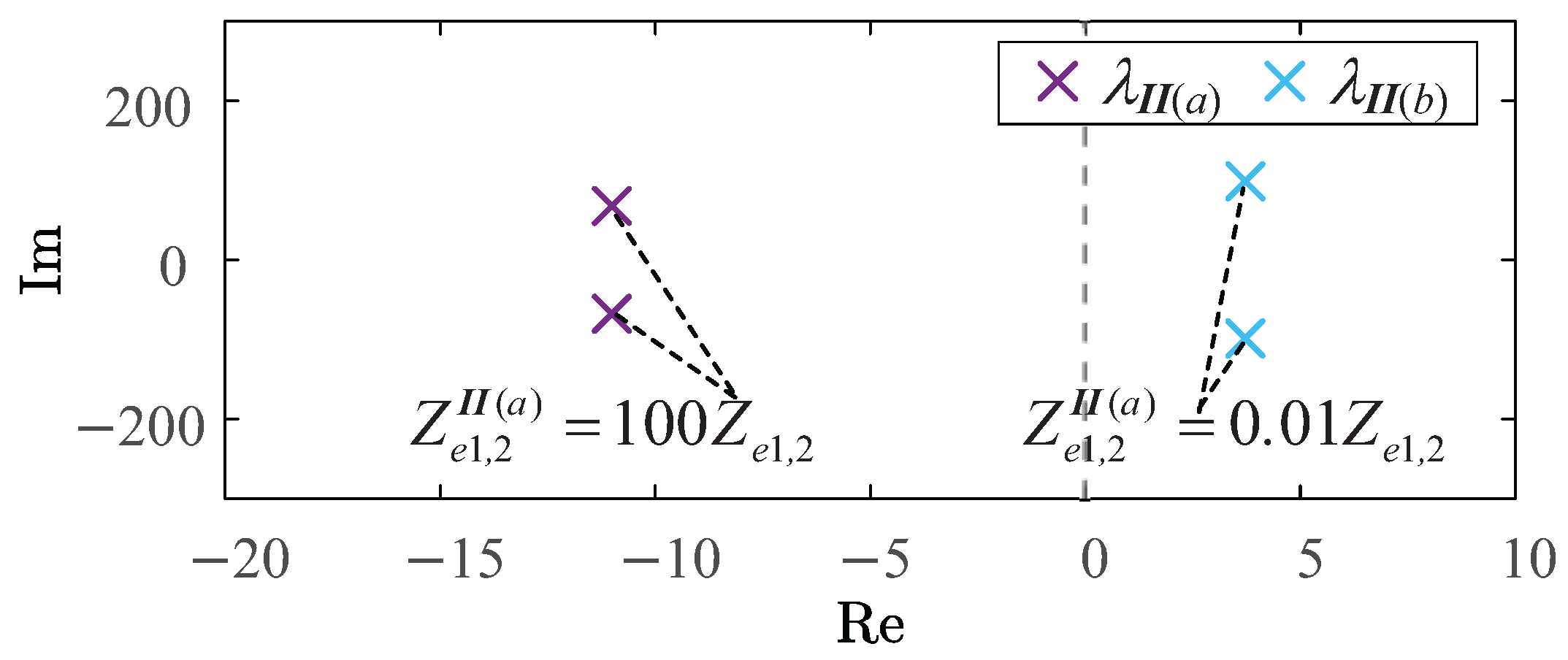
Using the initial parameters of Table 1 and taking $k_{p\mathrm{plll}1,2}=13.5$, $k_{i\mathrm{plll}1,2}=3000$ and $D_{\mathrm{m}1,2}=15$, the dominant eigenvalues of the GFL inverters are ${\lambda }_{23,24}=1.86\pm \mathrm{j}1.65\times {10}^3$. Under these parameters, doubling the connection impedance $Z_{e3,4}$ of the GFL inverters, the increase of the dominant eigenvalue $\Delta {\lambda }_{23,24}=0.12\pm \mathrm{j}0.3$ of the T1-type grid can be calculated by Equation (26). This indicates that as $Z_{e3,4}$ increases, the system eigenvalues move along the real axis to the RHP. The larger the connection impedance of the GFL inverters, the more likely the system is to lose stability. In contrast, using the initial parameters from Table 1 and taking $k_{p\mathrm{plll}1,2}=0.14$, $k_{i\mathrm{plll}1,2}=3.08$ and $D_{\mathrm{m}1,2}=7$, the dominant eigenvalues of the GFM inverters are ${\lambda }_{39,40}=3.47\pm \mathrm{j}98.17$. Under these parameters, doubling the coupling impedance $Z_{e1,2}$ of the GFM inverters produces a dominant increase in the eigenvalue $\Delta {\lambda }_{39,40}=-0.006\pm \mathrm{j}0.03$ for the T1-type grid via Equation (25). This demonstrates that increasing $Z_{e1,2}$ drives the eigenvalues to the left along the real axis, thus enhancing stability. The larger the connection impedance of the GFM inverters, the more stable the system is.

To verify the influence of the connection impedance on the stability of each inverter through simulation, T1-type grid topology structure is selected for research, as shown in Figure 4a. Four operating cases are defined as shown in

Table 5. Four connection impedance operating cases.

Case	${\mathit{Z}}_{\mathit{e}}$	${\mathit{k}}_{\mathit{p}\mathbf{plll}1,2}$ ${\mathit{k}}_{\mathit{i}\mathbf{plll}1,2}$	${\mathit{D}}_{\mathbf{m}1,2}$
$\mathit{I}\left(\mathit{a}\right)$	$Z_{e3,4}^{\mathit{I}\left(\mathit{a}\right)}=100Z_{e3,4}$ $Z_{e1,2}^{\mathit{I}\left(\mathit{a}\right)}=Z_{e1,2}$	13.5 3000	15
$\mathit{I}\left(\mathbf{b}\right)$	$Z_{e3,4}^{\mathit{I}\left(\mathbf{b}\right)}=0.01Z_{e3,4}$ $Z_{e1,2}^{\mathit{I}\left(\mathbf{b}\right)}=Z_{e1,2}$	13.5 3000	15
$\mathit{I}\mathit{I}\left(\mathit{a}\right)$	$Z_{e1,2}^{\mathit{I}\mathit{I}\left(\mathit{a}\right)}=100Z_{e1,2}$ $Z_{e3,4}^{\mathit{I}\mathit{I}\left(\mathit{a}\right)}=Z_{e3,4}$	0.14 3.08	7
$\mathit{I}\mathit{I}\left(\mathbf{b}\right)$	$Z_{e1,2}^{\mathit{I}\mathit{I}\left(\mathbf{b}\right)}=0.01Z_{e1,2}$ $Z_{e3,4}^{\mathit{I}\mathit{I}\left(\mathbf{b}\right)}=Z_{e3,4}$	0.14 3.08	7

.

In four operating cases, the electrical distance between the GFL inverters and the PCC changes under conditions $\mathit{I}\left(\mathit{a}\right)$ and $\mathit{I}\left(\mathbf{b}\right)$. Compared to conditions $\mathit{I}\left(\mathit{a}\right)$ and $\mathit{I}\left(\mathbf{b}\right)$, the electrical distance between the GFL inverters and the PCC remained the same under conditions $\mathit{I}\mathit{I}\left(\mathit{a}\right)$ and $\mathit{I}\mathit{I}\left(\mathbf{b}\right)$, while the electrical distance between the GFM inverters and the PCC changed. The small signal analysis of the four operating cases’ eigenvalues are presented in

Table 6. The dominant eigenvalue of under four operating cases.

Case	$\mathit{\lambda }$	f (Hz)	$\mathit{\zeta }$ (%)	Participation Factor (>0.1)
$\mathit{I}\left(\mathit{a}\right)$	${\lambda }_{23,24}=1.21\times {10}^2$ $\pm \mathrm{j}1.35\times {10}^3$	$215.1$	$-0.0894$	${\delta }_{\mathrm{l}1,\mathrm{l}2}=0.1320$ $i_{gq}=0.2339$
$\mathit{I}\left(\mathbf{b}\right)$	${\lambda }_{23,24}=1.67$ $\pm \mathrm{j}1.65\times {10}^3$	$262.8$	$-0.0010$	${\delta }_{\mathrm{l}1,\mathrm{l}2}=0.1783$ $i_{gq1,2}=0.2079$
$\mathit{I}\mathit{I}\left(\mathit{a}\right)$	${\lambda }_{39,40}=-11.01$ $\pm \mathrm{j}67.71$	$10.8$	$1.7670$	${\delta }_{\mathrm{m}2}=0.6209$ ${\omega }_{\mathrm{m}1}=0.2469$ ${\omega }_{\mathrm{m}2}=0.2324$
$\mathit{I}\mathit{I}\left(\mathbf{b}\right)$	${\lambda }_{39,40}=3.7195$ $\pm \mathrm{j}98.62$	$15.7$	$-0.1402$	${\delta }_{\mathrm{m}2}=0.5592$ ${\omega }_{\mathrm{m}1}=0.2206$ ${\omega }_{\mathrm{m}2}=0.2303$

.

The dominant eigenvalues of the GFL inverters under operating conditions $\mathit{I}\left(\mathit{a}\right)$ and $\mathit{I}\left(\mathbf{b}\right)$ are plotted in Figure 14. The eigenvalues of $\mathit{I}\left(\mathit{a}\right)$ are observed to be farther to the right compared to $\mathit{I}\left(\mathbf{b}\right)$, indicating that the larger the connection impedance of the GFL inverters, the more unstable the system is, which is consistent with the analysis results of $\Delta {\lambda }_{23,24}$ mentioned above.

The whole participation factors of the two pairs of eigenvalues are calculated and represented by colored dots as shown in Figure 15. The participation degree of $i_{gq}$ is highest in both cases, with $\mathit{I}\left(\mathbf{b}\right)>\mathit{I}\left(\mathit{a}\right)$. This implies that a shorter electrical distance between the GFL inverters and the PCC amplifies the grid-induced impacts on the GFL dynamics. The participation degree of ${\delta }_{\mathrm{l}1,\mathrm{l}2}$ under $\mathit{I}\left(\mathit{a}\right)$ exceeds that of $\mathit{I}\left(\mathbf{b}\right)$, suggesting that the longer electrical distance reduces interactions between GFL units.

The dominant eigenvalues of the GFM inverters under operating conditions $\mathit{I}\mathit{I}\left(\mathit{a}\right)$ and $\mathit{I}\mathit{I}\left(\mathbf{b}\right)$ are plotted in Figure 16. The eigenvalues of $\mathit{I}\mathit{I}\left(\mathit{a}\right)$ are observed to be farther to the left than $\mathit{I}\mathit{I}\left(\mathbf{b}\right)$, indicating that the larger the connection impedance of the GFM inverter, the more stable the system, which is consistent with the analysis results of $\Delta {\lambda }_{39,40}$ mentioned above.

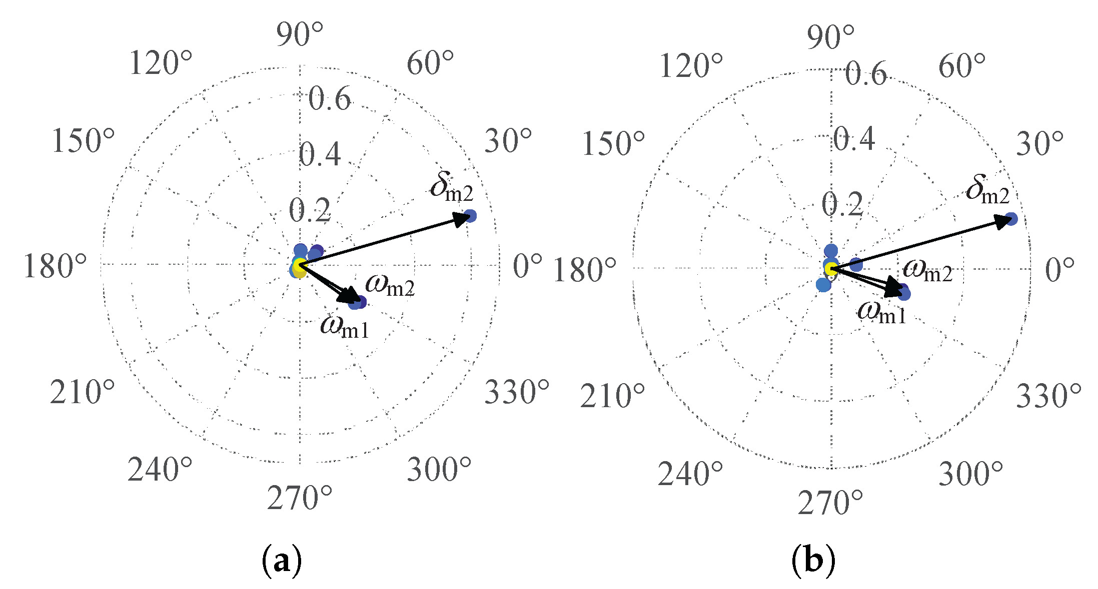
The whole participation factors of the two pairs of eigenvalues are calculated and represented by colored dots as shown in Figure 17. In $\mathit{I}\mathit{I}\left(\mathit{a}\right)$, the participation degrees of ${\delta }_{\mathrm{m}2}$ and ${\omega }_{\mathrm{m}1,2}$ are higher than those of $\mathit{I}\mathit{I}\left(\mathbf{b}\right)$. This indicates that increasing the electrical distance between GFM inverters and PCC amplifies inter-inverter interactions and elevates the influence of their intrinsic frequency stability on system dynamics.

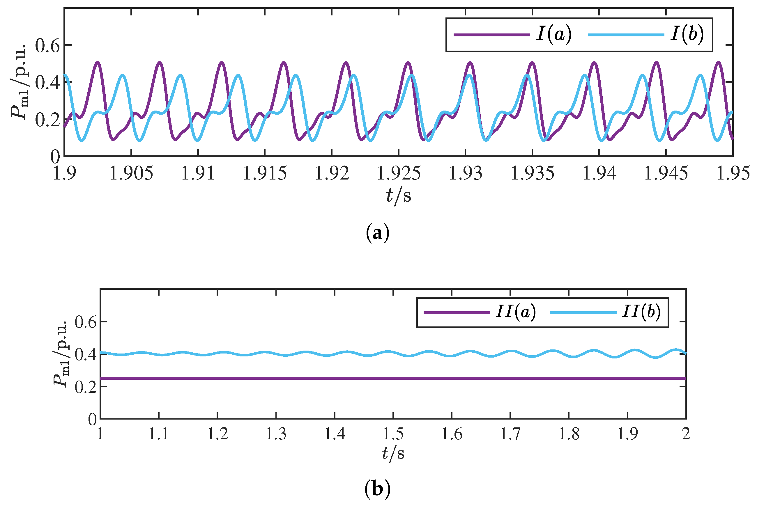
Figure 18 presents the time domain simulation results of the normalized active power $P_{\mathrm{m}1}$ of the GFM1 inverter under four connection impedance operating cases. In Figure 18a, it can be seen that both curves exhibit oscillations that diverge over time, but the blue curve diverges more slowly. This indicates that the system damping ratios under both operating scenarios are less than 0. In Figure 18b, it can be seen that the purple curve does not have oscillation, while the blue curve exhibits oscillation that diverges over time. This indicates that the damping ratio of the system is greater than 0 under condition $\mathit{I}\mathit{I}\left(\mathit{a}\right)$ and less than 0 under condition $\mathit{I}\mathit{I}\left(\mathbf{b}\right)$. The time domain results are consistent with the analysis results of $\zeta$ in Table 6.

The same analysis and verification are performed under grid topology structures of T2- and T3-type. The results show that as the connection impedance increases, the GFL inverters are more prone to oscillation, and the system stability declines. In contrast, the GFM inverters are less likely to oscillate, and the system stability increases.

5. Conclusions

This paper establishes full-order state-space models for three typical grid topologies: radial, ring, and meshed networks, and systematically analyzes the impacts of these grid topology structures on the dominant oscillatory modes of the GFL and GFM inverters. In addition, the influence of inverter connection impedance on these dominant oscillatory modes is investigated. Compared to previous studies, the state-space model developed in this paper is more universal and easier to extend. Earlier research only focused on building state-space models for a limited number of GFM and GFL inverters, while our model theoretically allows for an unlimited number of both types of inverters. Furthermore, early studies mainly focused on the impact of inverter internal parameters on system small-signal stability, while neglecting the influence of external grid topology structure on system stability. This study emphasizes the impact of different grid topology structures on the small signal stability of inverters, an aspect that received less attention in prior analyses of grid topology impacts. Based on the findings, the following conclusions are derived:

• The GFL inverters are significantly influenced by grid conditions and are more suitable for integration into strong grid topology structures such as ring- or meshed-type topologies.
• The GFM inverters are less affected by the power grid and are more critically dependent on their synchronization control capabilities. Enhancing the synchronization mechanisms of GFM inverters through design or retrofitting can improve the small signal stability of system.
• The lower connection impedance for GFL inverters and the higher connection impedance for GFM inverters improve overall system stability.

Future power systems will gradually upgrade and interconnect traditional radial and ring-type grids while developing more flexible and stable meshed grid architectures. When integrating renewable energy sources, GFM inverters that are less affected by the power grid can be given priority. When GFL inverters must be used, it is advisable to connect them to a ring- or meshed-type power grid with a strong grid capacity. Additionally, system stability can be improved by placing the GFL inverters closer to the PCC and positioning the GFM inverters farther from the PCC to leverage impedance decoupling effects. Finally, we plan to extend this research to larger real-world power grids in the future, including large-scale power systems with radial, ring, and mesh grid topology structures. Additionally, practical factors such as aging characteristics of power electronic devices, communication delays, and other influencing elements must be incorporated into the stability analysis of grid-connected inverter systems. Additionally, the oscillation mechanisms induced by inverters in hybrid systems and their propagation characteristics deserve in-depth investigation. This expansion aims to strengthen the foundational research supporting the secure and stable operation of power systems.