A Scheduling-Optimization Model with Multi-Objective Constraints for Low-Carbon Urban Rail Transit Considering the Built Environment and Travel Demand: A Case Study of Hangzhou

Abstract

Urban rail transit, a crucial component of urban public transportation, often experiences increased operational costs and carbon emissions due to low-load operations being conducted during off-peak passenger flow periods. This study aims to develop an optimization method for the daily scheduling of rail train operations with the goal of carbon emission reduction, while comprehensively considering the built environment and travel demand. Firstly, the influence of the urban built environment on residents’ travel demand is analyzed using an XGBoost model. Secondly, a time convolutional travel demand prediction model, Built Environment-Weighted Temporal Convolutional Network (BE-TCN), weighted by built environment factors, is constructed. Finally, an optimization method for rail train operation schedules based on the built environment and travel demand is proposed, with the objective of carbon emission reduction. A case study is conducted using the Hangzhou urban rail transit system as an example. The results indicate that the optimization method proposed in this study can achieve monthly carbon emission reductions of 1524.58 tons, 1181.94 tons, and 520.84 tons for Lines 1, 2, and 4 of the Hangzhou urban rail transit system, respectively. The research findings contribute to enhancing the economic efficiency and environmental sustainability of urban rail transit systems.

1. Introduction

As a crucial mode of low-carbon transportation, urban rail transit faces a prominent issue of supply–demand imbalance during off-peak hours [1,2]. Existing research indicates that the average load factor during off-peak periods in major cities in China is less than 30%, yet the trains continue to operate on fixed schedules, resulting in 20–30% of their mileage being wasted on ineffective runs and significant energy inefficiency. The carbon emission intensity per passenger-kilometer during off-peak periods is 40–60% higher than during peak hours [3,4], which leads to an annual carbon redundancy exceeding 6 million tons of CO₂. Traditional static scheduling models struggle to adapt to the characteristics of the built environment and dynamic travel demand fluctuations [5], such as tidal passenger flows and holiday travel patterns. Therefore, developing intelligent scheduling methods based on dynamic demand prediction is conducive to improving the energy efficiency of rail transit and assisting in the achievement of the “dual carbon” goals. Currently, the research on the low-carbon operation and planning of urban rail transit is increasingly focusing on the coupling relationship between the built environment and transportation systems. However, existing modeling methods still exhibit significant limitations in characterizing the heterogeneous impacts between rail stations. Most studies, by employing static POI-weighted or historical average prediction methods, fail to fully account for the dynamic differences among stations in terms of their passenger flow, land use, energy consumption, and carbon emission characteristics, which results in limited model accuracy and applicability. Jia et al. [6] and Chen et al. [7] quantified the environmental benefits of rail transit from the perspectives of carbon reduction and energy consumption prediction, respectively, but relied on static POI-weighted or historical average methods [8], which inadequately capture the dynamic influence of functional differences among stations on their passenger flow and energy consumption. Studies that utilized causal inference and spatial network analysis have uncovered the relationship between the built environment and passenger flow [9,10], but these models operate under the assumption of homogeneous effects across stations while overlooking the differentiated interaction effects that stem from varying locations. Some scholars have attempted to introduce dynamic analytical frameworks to improve heterogeneity modeling. Lei et al. [11] and Wen et al. [12] optimized traffic demand prediction from the perspectives of spatiotemporal context and dynamic demand, respectively, but did not systematically integrate the multidimensional dynamic characteristics of the built environment. Research on energy efficiency [13] has refined the analysis of energy consumption differences between different train tractions and station operations, yet the modulating effects of environmental heterogeneity at the station level [14,15] on energy consumption remain insufficiently modeled. Future research needs to further integrate dynamic data and heterogeneity modeling methods to more accurately reflect the impact of inter-station differences on the environmental performance of rail transit. Niu et al.’s [16] collaborative energy-saving optimization model could be extended to scenarios with heterogeneous built environments, while Yuan et al.’s [17] proposed life-cycle carbon emission measurement framework requires refinement by incorporating station-level characteristic differences.

In recent years, the research in the field of public transportation system planning and management has been continuously deepening. Traditional static transit assignment models, which assume fixed bus stops, struggle to adapt to the dynamic changes encountered in actual operations [18]. In contrast, dynamic bus stop simulations can integrate the real-time passenger demand and traffic conditions [19]. By employing methods such as dynamic spatiotemporal multiscale representation, these simulations can more accurately predict passenger flows, optimize stop locations and operations, and adapt to the complexity and uncertainty of urban transportation [20]. In the realm of multi-objective transit network design, this problem is often framed as a set covering problem, which necessitates the simultaneous optimization of multiple objectives, including route coverage, operational costs, and service quality. Ahern et al. [21] proposed an approximate multi-objective optimization approach that integrates route design with service frequency settings. This approach also incorporates intelligent algorithms such as genetic algorithms and particle swarm optimization to enhance the solution’s efficiency and optimization effectiveness, and thereby offers new insights into transit network design. In the context of transit user assignment problems, the interval network representation method has gained prominence due to its ability to better reflect network uncertainty and complexity. For instance, Du et al. [22] introduced a Weibit sequence transit assignment model based on hyperpath graphs and generalized extreme value network representations. This model accounts for passengers’ travel choice behaviors and network dynamic characteristics. The applicability of this representation method in scenarios such as congested and multimodal transportation networks has also been explored, which has provided new perspectives and solutions for transit user assignment. These studies have advanced the scientific and refined planning and management of public transportation systems, offering new theories and methods for optimizing transit systems and providing valuable references for practical applications. With ongoing technological advancement and data accumulation, more breakthroughs are anticipated in the future.

In the field of low-carbon transportation scheduling and decision-making, optimization problems under multi-constraint coupling have attracted increasing attention. Traditional optimization models often focus on a single objective (e.g., energy consumption minimization), but actual operations require the coordinated optimization of multiple constraints, such as passenger waiting time thresholds, the travel demand, and grid carbon emission factors, which leads to significant conflicts among objectives. To address this issue, existing research has explored multi-objective optimization methods, scheduling strategies, and low-carbon constraint modeling. Some scholars have adopted multi-objective linear programming approaches. Li et al. [23] and Yuan et al. [24] optimized operational strategies from the perspectives of energy efficiency and service quality, and real-time scheduling and passenger flow control, respectively. Nakano et al. [25] proposed a low-carbon charging strategy for electric buses, emphasizing dynamic adjustments based on real-time conditions. Multi-objective linear programming has been used to optimize transportation structures and land use [26,27], but static modeling methods struggle to adapt to dynamic passenger flow fluctuations and energy supply–demand variations during peak hours. Efforts have also been made to introduce multi-objective optimization methods to balance conflicts among different constraints. Multi-objective optimization frameworks have been employed to coordinate public transport mode selection and carbon reduction goals [28,29], yet these approaches still rely on offline optimization and lack real-time dynamic adjustment capabilities. Evolutionary algorithms such as NSGA-II [30,31] can handle high-dimensional objective spaces, but their computational efficiency and adaptability to complex dynamic environments remain insufficient. Ning et al. [32] proposed a multi-agent reinforcement learning (MARL)-based train scheduling method to dynamically optimize the energy consumption and operational efficiency of train scheduling, but the impact of grid low-carbon scheduling (e.g., time-of-use pricing and renewable energy integration) on operational decisions has not been thoroughly analyzed. Although Wang et al.’s [33] data mining model can predict residents’ low-carbon travel patterns, this model has not been integrated into a closed-loop feedback system with real-time scheduling.

There are some limitations in the existing research. Traditional optimization models and certain multi-objective linear programming methods exhibit static characteristics, making it difficult for them to effectively adapt to the dynamic changes in passenger flow and energy supply-demand during peak hours. Although multi-objective optimization frameworks have been explored, most of them still rely on offline optimization and lack real-time dynamic adjustment capabilities, particularly under complex dynamic conditions such as sudden passenger surges and grid-load fluctuations.

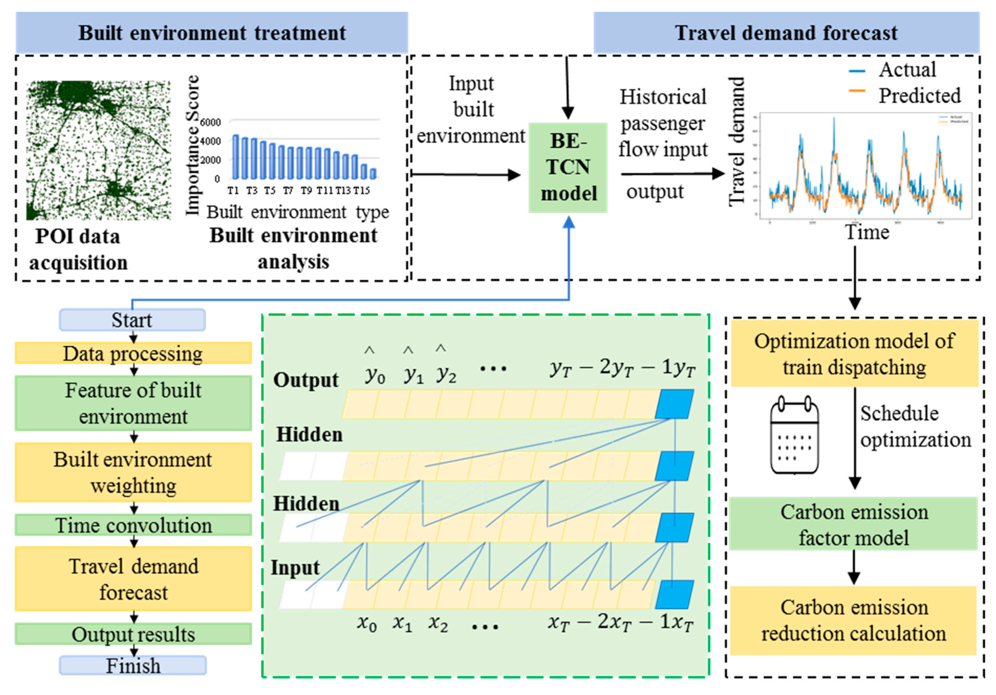
A scheduling framework with multi-objective constraints is proposed in this study. First, to address the interaction between urban residents’ travel demand and the built environment, a Built Environment-Time Convolutional Network (BE-TCN) is constructed, which dynamically incorporates built environment factors by assigning weights to them based on their differential influence on the travel demand, while also incorporating historical travel data, to achieve the precise prediction of future travel demand. Second, an optimization model for urban rail transit daily operation scheduling is developed based on the predicted travel demand; further, it fully considers constraints such as the passenger waiting time and train capacity, aiming to minimize the number of train dispatches and achieve an optimal carbon reduction solution. Finally, the proposed methods are validated using a dataset from Hangzhou urban rail transit. The research methodology is illustrated in Figure 1. This paper contributes meaningfully to the field of multi-objective scheduling by introducing an integrated framework. This framework aims to enhance the accuracy of passenger flow forecasting through the application of the BE-TCN model, which effectively captures spatiotemporal patterns. It also strives to achieve a more balanced optimization of operational efficiency, carbon footprint reduction, and passenger satisfaction within real-time scheduling. Additionally, this paper offers an in-depth analysis of the interrelationship between the built environment and passenger flow, proposing practical strategies that could potentially support sustainable transportation planning. The findings of this study provide scientific decision-making support for urban rail transit managers in the formulation of differentiated train operation plans that align with travel demand, and thereby contributes to the promotion of carbon emission reduction in urban rail transit systems.

2. Methods

2.1. Data Sources and Processing

In this study, built environment PIO data of Hangzhou’s rail transit stations were collected, as well as the passenger flow data from entrance/exit gate counters on the operational routes of 74 stations for the period from 1 January 2019 to 25 January 2019. These datasets underwent rigorous cleaning and classification, including temporal segmentation (by time periods) and entry/exit differentiation, followed by data preprocessing steps such as standardization and normalization. The station attraction areas were determined based on a combination of factors including commercial facilities, public service facilities, green spaces and squares, work offices, business residences, and residential land use. The built environment data of Hangzhou’s urban rail transit stations are shown in

Table 1. Built environment data for subway stations in Hangzhou.

Variable			Average Value	Standard Deviation	Minimum	Maximum
Land use characteristics	Commercial facilities	Catering services	425.08	289.59	2	887
		Shopping service	572.10	333.22	9	890
		Accommodation services	69.99	86.85	0	434
		Life service	2004.33	1242.82	28	3777
		Sports leisure service	64.60	55.67	1	209
	Public service facilities	Health care services	68.14	63.70	1	250
		Scientific, educational and cultural services	154.90	137.90	0	448
		Public fitness services	34.45	43.08	0	259
	Greenland square	Scenic spots	9.56	18.65	0	115
	Work Office	governmental agencies	104.01	116.49	3	394
		Financial and insurance services	69.03	68.99	0	266
		Corporate enterprise	1034.71	812.66	12	2359
		industrial park	3.10	3.35	0	15
	Business residence	Building related	21.56	23.47	0	79
	Residential land	Residential area	125.24	196.69	0	872
	Transportation hub	Transportation facilities service	220.53	181.93	10	658

. Due to the large number of stations (74 in total), for each of which the data include entry/exit IDs and the number of passengers entering during different time periods (5 min intervals), only the passenger entry numbers for stations 0–10 during the 7:00–8:00 time period are shown in

Table 2. The number of passengers entering stations 0–10 from 7:00 to 8:00.

Entry Gate ID Number	Site ID
time	0	1	2	3	4	5	6	7	8	9
7:00–7:05	13	7	13	8	13	7	15	52	18	63
7:05–7:10	17	7	12	7	25	20	10	41	19	60
7:10–7:15	5	6	25	15	35	19	16	94	18	60
7:15–7:20	8	7	13	7	26	21	19	40	20	106
7:20–7:25	13	14	13	13	39	21	17	75	25	129
7:25–7:30	18	4	20	11	13	28	17	134	22	90
7:30–7:35	7	7	12	15	54	39	11	140	52	86
7:35–7:40	1	8	32	20	25	23	31	89	26	166
7:40–7:45	30	18	6	8	50	44	25	115	29	146
7:45–7:50	11	7	22	16	57	44	19	156	42	142
7:50–7:55	15	6	31	12	58	40	41	187	61	122
7:55–8:00	20	11	25	13	45	38	43	96	44	208

.

2.2. Construction of XGBoost Model Based on the Impact of Built Environment on Residents’ Travel Demand

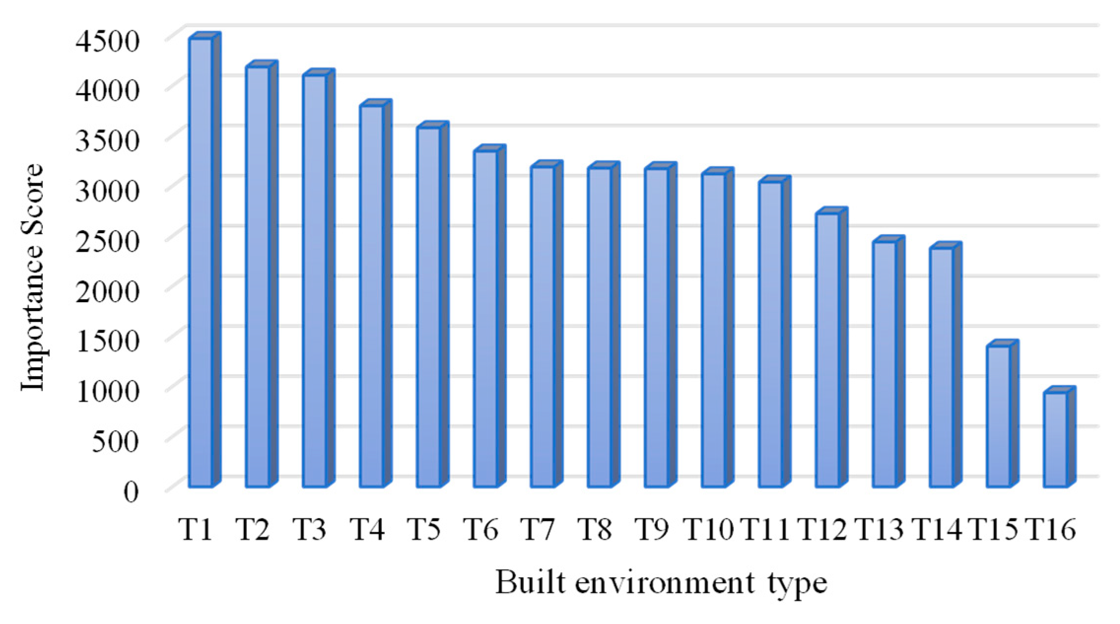
XGBoost is an efficient gradient-lifting decision tree model that is widely used in the field of large-scale data analysis. This model has enhanced prediction accuracy due to optimizing the loss function and capturing complex nonlinear relationships. This model incorporates a built-in feature importance scoring function that allows for the intuitive evaluation of variable impacts on specific objectives. By leveraging L1 and L2 regularization techniques, the model effectively manages the process’s complexity and curtails the risk of overfitting, which thereby enhances its robustness. Additionally, the model boasts strong visualization capabilities, which facilitate easy interpretation of the results. This model helps to capture the complex relationship between the built environment and travel demand and accurately identify the key influencing factors. Therefore, this paper discusses the impact of the built environment on residents’ travel demand based on the XGBoost model.

The model construction steps are as follows: First, the built environment data are divided into a training set and a testing set in a ratio of 70/30%. Secondly, the model is optimized by adjusting the regularization parameter, sampling strategy, and learning rate to enhance its performance and prevent overfitting. The training process is configured to run for 5000 iterations. Finally, the number of times that each built environment-related feature is used to split nodes across all decision trees is added up, and the weights of each feature in all decision trees are considered comprehensively to evaluate the importance of the built environment features. The parameters of the XGBoost model are presented in

Table 3. Parameters of the XGBoost model.

Weight of L2 Regularization Term	Sample Proportion of Random Sampling	Scale of Randomly Selected Features	Minimum Sample Weight Sum of Child Nodes	Learning Rate	Specify the Number of Threads Used	Loss Reduction During Control Node Splitting
10	0.75	0.75	2	0.03	8	0.15

.

The calculation method of the importance score of the XGBoost model is shown in Equation (1):

$$I_i=\sum _{j=1}^n{C}_{ij}$$

(1)

where $I_i$ is the importance score; $n$ represents the total number of trees; $C_{ij}$ is the number of times that feature i is used to split nodes in the jth tree.

2.3. BE-TCN Model Construction of Urban Residents’ Travel Demand Prediction Based on Built Environment Weighting

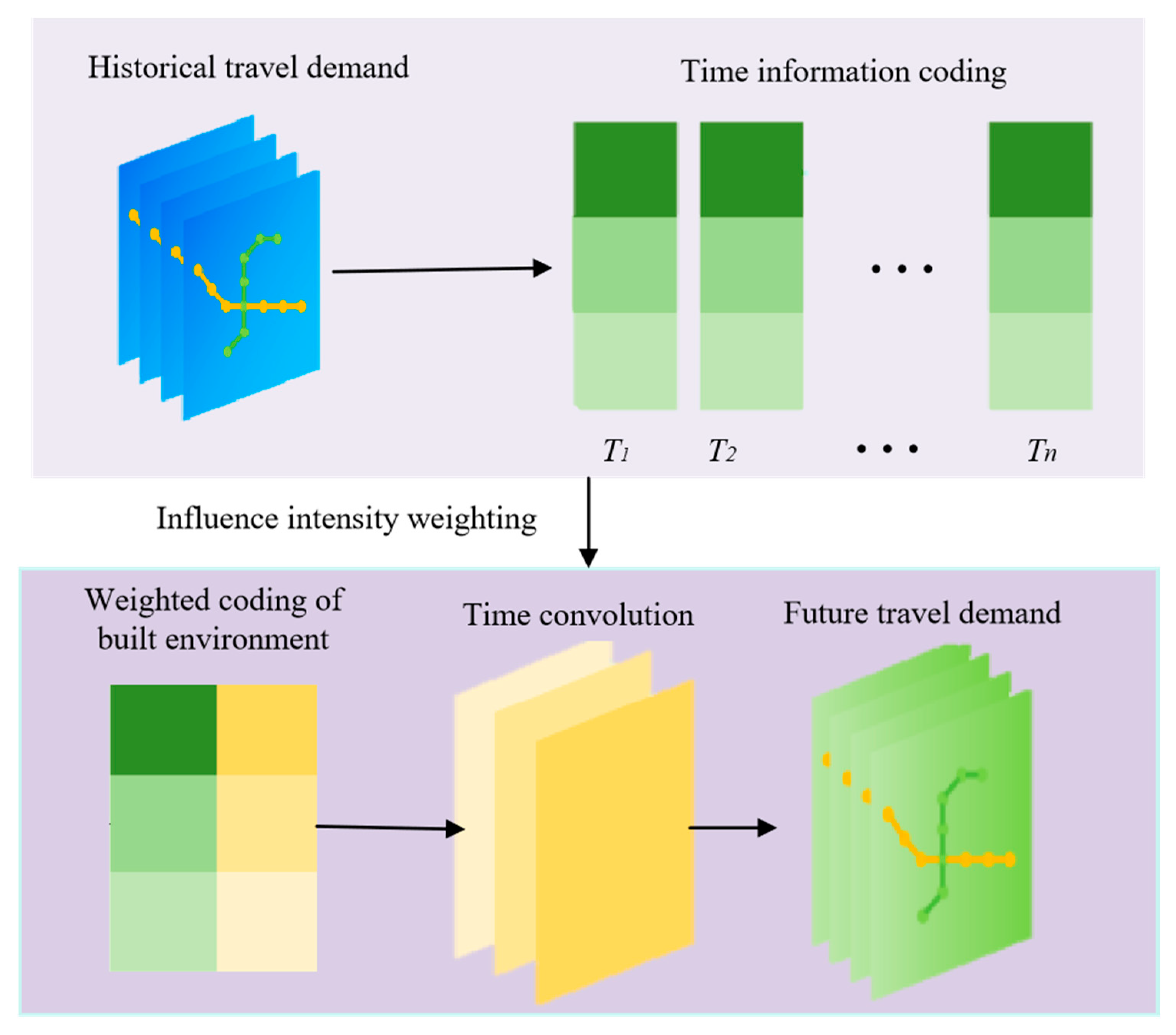
To investigate the differential impacts of the built environment on urban rail transit travel demand, the BE-TCN model, a weighted prediction framework that accounts for the varying intensity of the influence of the built environment, is proposed. The model incorporates a weighting mechanism that uses the intensity of built environment influences as weights to accurately depict the patterns of demand variation. By leveraging the advantages of temporal convolutional networks, the BE-TCN model effectively captures long-term dependencies in time-series data, achieving a significantly enhanced prediction accuracy and robustness. Additionally, this model supports the fusion of multi-dimensional features, including built environment indicators, historical travel data, and temporal information, to comprehensively represent complex travel scenarios and provide reliable technical support for urban rail transit demand prediction.

The BE-TCN model, a temporal convolutional network architecture, is designed for the forecasting of future travel demand. Initially, historical travel demand data are encoded into a sequential temporal information format. Subsequently, weighted encoding mechanisms are applied to incorporate the influence of the built environment. The encoded data are then processed through temporal convolutional layers to extract features at various time scales, facilitating the generation of future travel demand predictions. The diagrammatic representation below outlines the key stages of the process: historical travel demand data are transformed into temporal information; weighted encoding of the built environment enhances the model’s consideration of environmental factors; and temporal convolution operations on these encodings enable future travel demand prediction. The framework of the BE-TCN model is illustrated in Figure 2.

2.3.1. TCN Model

$O_t$ is the objective function at time t, and is calculated by Equation (2):

$$O_t=TCN(X_t,\theta )$$

(2)

where $X_t$ is the input data at time t; $\theta$ is the model parameter.

2.3.2. Built Environment Weighting

In the built environment weighting, ${\mathrm{F}}_{\mathrm{w}\mathrm{e}\mathrm{i}\mathrm{g}\mathrm{h}\mathrm{t}}$ is the sum of the weighted feature predictions, as show in Equation (3):

$$F_{weight}=\sum _{i=1}^n{w}_i*F_i$$

(3)

where $w_i$ is the weight related to the ith variable$; F_i$ is the predicted output of the ith variable.

2.3.3. Predictive Output

$Y_{pred}$ is the predictive output$; \mathsf{\sigma }$ is the activation function, as shown in Equation (4):

$$Y_{pred}=\mathsf{\sigma }\left(TCN\right(X_t,\theta )+F_{weight})$$

(4)

2.3.4. Error Indicators

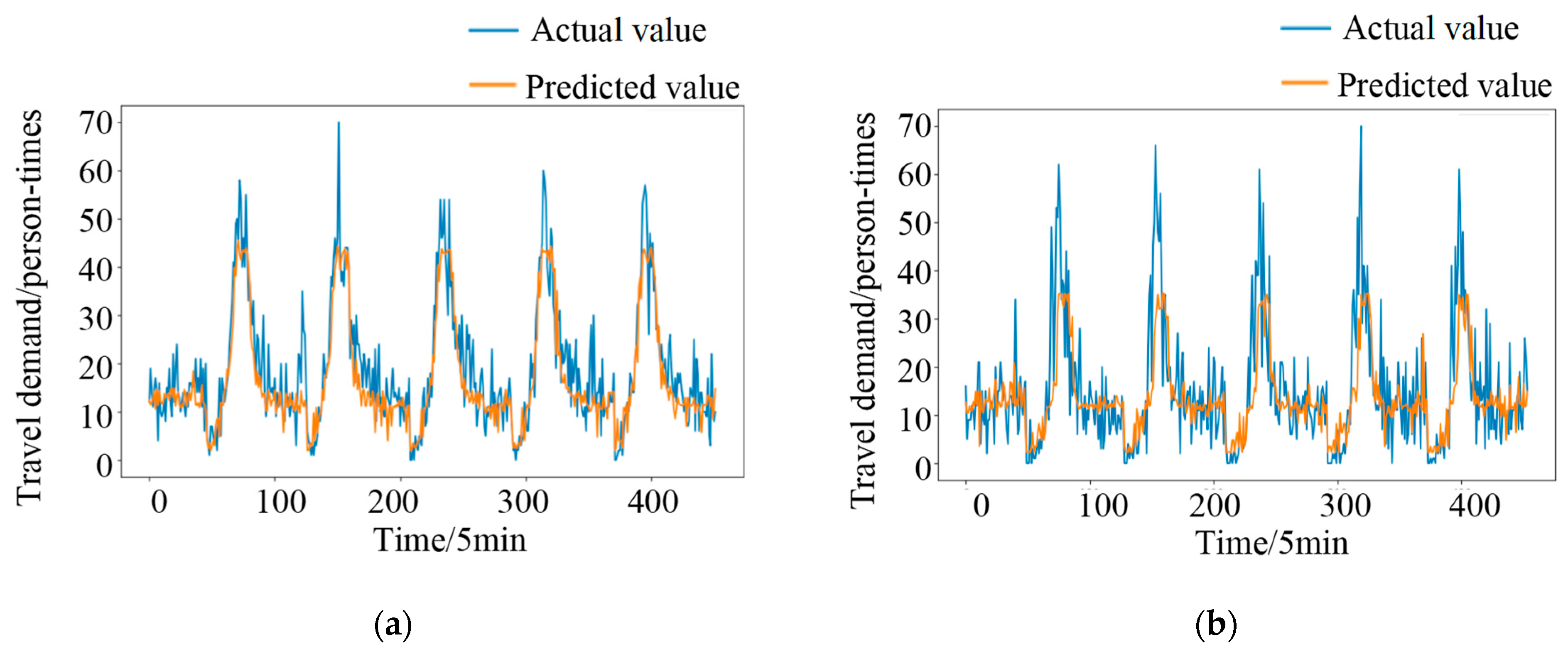
Mean absolute error (MAE) and root mean squared error (RMSE) were used to evaluate the prediction results of the model, as shown in Equations (5) and (6), where $y_i$ is the actual value; ${\mathrm{y}}_{\mathrm{i}}^{\prime }$ is the predicted value; n is the number of samples.

$$MAE={\displaystyle \frac{1}{n}}\sum _{i=1}^n\left|y_i-y_i^{\prime }\right|$$

(5)

$$RMSE=\sqrt{{\displaystyle \frac{1}{n}}\sum _{i=1}^n{(y_i-y_i^{\prime })}^2}$$

(6)

2.4. Construction of an Optimization Model for Urban Rail Transit Train Scheduling Considering Carbon Emission Reduction

To achieve the carbon emission reduction targets and enhance the operational efficiency of urban rail transit systems, this paper constructs an optimization model for urban rail transit train scheduling that considers carbon emission reduction objectives. Firstly, an objective function is devised with the overarching goals of minimizing train service frequency, passenger waiting times, and carbon emissions. Corresponding weights are allocated to these distinct objectives to reflect their relative importance. Secondly, optimization constraints are established, including the passenger waiting time, operational time intervals, and suitable train passenger capacities, to ensure the feasibility of the train scheduling plan. Finally, a linear programming model is employed to solve the optimization model. This approach aims to achieve more efficient and environmentally friendly urban rail transit operations.

2.4.1. Objective Function

In this study, the mixed-integer linear programming (MILP) methodology was adopted to address the optimization model, in which Pyomo, an open-source modeling framework implemented in Python 3.9.13, was also integrated. Regarding the solver selection, CBC, a widely recognized open-source solver for linear and mixed-integer linear programming problems, was employed.

With respect to the determination of weight settings, extensive reference was made to the pertinent literature within the field, and consultations were conducted with domain experts. Zhu, C. et al. [34] and Yu, D. et al. [35] presented valuable reference methodologies for choosing weight settings in analogous problems. Furthermore, given the practical application context, in-depth discussions were undertaken with experts to achieve a balanced consideration of the impacts of the number of departures, the volume of waiting passengers, and carbon emissions within the objective function, which allowed us to delineate a reasonable range for the weights.

To evaluate the computational efficiency of the solution approach, the computation time for each experimental run was meticulously recorded. Ultimately, the resultant scheduling timetable was preserved for subsequent analytical procedures and practical applications.

The preparation of the urban rail transit train operation plan included three optimization objectives: minimum departure times, passenger waiting time, and carbon emissions. The objective function $Z$ is calculated using Equation (7):

$$Maximize Z=\alpha \sum _{l\in L}\sum _{t\in T}{x}_{lt}+\beta \sum _{s\in S}\sum _{t\in T}{n}_{st}+\gamma \sum _{l\in L}\sum _{t\in T}{\left({CeO}_y\right)}_l$$

(7)

where the system decision variable ${\mathrm{x}}_{\mathrm{l}\mathrm{t}}$ indicates whether the line $l$ sends out the train at time $\mathrm{t}$; $n_{st}$ is the waiting time $t$ at station $S$; $L$ is the collection of Hangzhou urban rail transit train lines; $T$ is the time period for preparing the operation plan; $S$ is the set of stations $s$ on the line; ${\left({CeO}_y\right)}_l$ refers to the carbon emissions consumed by the train running once on line l.

2.4.2. Constraint Condition

• Judge whether the train is sent out at time $\mathrm{t}$: $x_{lt}\in \left\{\mathrm{0,1}\right\}$ is whether the train is sent out at time t on a given line.

$$x_{lt}\left\{\begin{array}{c}1 Departure\\ 0 No departure\end{array}\right.$$

(8)

2.

Passenger waiting time constraints: passenger flow entering station S at time $\mathrm{t}$ of $D_{s,t}$; $y_{ls,t-t^{\prime }}$ indicates whether the train $x_{l{t}^{\prime }}$ sent at time $t^{\prime }$ arrives at station $\mathrm{S}$ at time $t^{\prime }$; $t_0$ is the arrival time.

$$n_{st}=n_{s,t-1}+D_{s,t}-\sum _{l\in L}\sum _{t^{\prime }\le t}{x}_{l{t}^{\prime }}*y_{ls,t-t^{\prime }}$$

(9)

$$n_{st}\ge 0, \forall \mathrm{s}\in {\mathrm{S}}^{\prime }, t-t^0\in W_{max}$$

(10)

$$x_{lt}\left\{\begin{array}{c}1 The train arrives S at time t\\ 0 The train does not arrive S at time t\end{array}\right.$$

(11)

3.

Operation time interval constraints: $I_{min}$ is the minimum departure interval.

$$x_{lt}+x_{l{t}^{\prime }}\le 1 ,\forall \mathrm{l}\in \mathrm{L}$$

(12)

$$\left|t-t^{\prime }\right|\le I_{min}$$

(13)

4.

Suitable passenger capacity of train: $a_{lt}$ passenger flow boarding the line $\mathrm{l}$ at time $\mathrm{t}$; $\mathrm{C}$ is the maximum passenger capacity of the train, and in this study, $\mathrm{C}=1450$. To ensure passenger comfort, the appropriate passenger capacity of the train is 80% of the maximum passenger capacity.

$$\left|a_{lt}\right|\le 0.8C, \forall \mathrm{s}\in {\mathrm{S}}^{\prime }, \mathrm{t}\in \mathrm{T}$$

(14)

2.5. Construction of Carbon Emission Factor Model of Urban Rail Transit

Carbon emissions are generated by traction electricity consumption during the operation of urban rail transit systems [36]. A top-down approach is employed to calculate carbon emissions by analyzing the electricity consumption data and power emission factors of the urban rail transit system. The carbon emission factor model integrates the passenger flow demand forecast, operation characteristics, vehicle energy consumption, and carbon emission conversion coefficient of grid power generation to provide accurate carbon emission estimation. When calculating the indirect emissions from purchasing electricity, public institutions usually use the average emission factor of the national grid as a reference. This study selects the value (0.6101 tCO₂/mwh) provided by the national development and reform commission in their guidelines for accounting methods and reporting related to greenhouse gas emissions for enterprises from 2013 to 2015 to calculate the indirect emissions corresponding to the purchase of electricity [37].

Carbon emissions due to traction power consumption during urban rail transit operation: ${\left({CeO}_y\right)}_l$ represents the total carbon emissions during the operation phase of urban rail transit trains, as shown in Equation (15):

$${\left({CeO}_y\right)}_l=U_t{*E}_{k,e}$$

(15)

where $U_t$ represents the traction energy consumption of urban rail transit trains, in kW·h; $E_{k,e}$ represents the electricity emission factor (average level of the national power grid), in kg ${CO}_{2}e$/kW·h.

The input data for the model include the following: an inbound passenger flow matrix, recorded at 5 min intervals and expanded to 1 min intervals; an outbound passenger flow matrix, also recorded at 5 min intervals and expanded to 1 min intervals; and an inter-station time matrix, which contains the station numbers and their corresponding running times for each line. Additionally, the station number ranges for three lines—Line 1, Line 2, and Line 4—are defined, and the maximum passenger capacity of the trains is set at 1450 people. The weighting parameters α, β, and γ are set to 40%, 40%, and 20%, respectively, to balance the impacts of the number of departures, the number of waiting passengers, and carbon emissions in the objective function.

3. Results

3.1. Analysis of Impact Intensity of Built Environment on Residents’ Travel Demand Based on XGBoost Model

The impact intensity analysis of the influence of the built environment on urban rail transit travel based on the XGBoost model is shown in Figure 3. The abbreviations for the built environment type used in Figure 3 are shown in

Table 4. The abbreviations for the built environment types.

Acronym	Variable
T1	Catering services
T2	Shopping service
T3	Scenic spots
T4	Health care services
T5	Accommodation services
T6	Scientific, educational and cultural services
T7	governmental agencies
T8	Sports leisure service
T9	Public fitness services
T10	industrial park
T11	Building related
T12	Residential area
T13	Financial and insurance services
T14	Corporate enterprise
T15	Corporate enterprise
T16	Life service

. There are significant differences in the intensity of the impacts of different built environment types on urban rail transit travel. It can be seen from Figure 3 that the importance score of the built environment of Hangzhou urban rail transit stations covers multiple service and facility categories.

A SHAP plot is shown in Figure 4. According to the analysis of the SHAP value plots, there are significant differences in the impact of various features on the model’s output. In particular, features T1 and T2 exhibit a wide distribution of SHAP values, indicating that these features have a substantial influence on the model’s predictive outcomes. For feature T1, high feature values tend to increase the model’s output, exerting a positive impact, whereas low feature values tend to decrease the model’s output, resulting in a negative impact. In contrast, the effects of high and low feature values for feature T2 on the model’s output are more balanced, although high feature values still show a slight positive influence overall. Additionally, some features, such as T3 and T4, have a relatively concentrated distribution of SHAP values, suggesting that these features have a smaller or more consistent impact on the model’s output.

The main conclusions are as follows:

• The catering service score is nearly 4500, highlighting its importance in meeting the basic needs of passengers, especially for long-time commuters and diners;
• The scores of shopping services and scenic spots exceeded 4000, indicating that the traffic flow at the stations near such places is high, and highlighting the dependence of these environment types on the urban rail transit system, and emphasizing the key role of effective transportation connection in supporting the development of commerce and tourism;
• The scores of medical care, accommodation, science, education, culture, and government agency services are all above 3000, which shows that such services occupy a core position in daily life and have a strong interdependence with the public transport system;
• The score of sports leisure and public fitness services is slightly lower than 3000, indicating that the frequency of use of such facilities is relatively low compared with that of daily essential services;
• The score of industrial parks and buildings is about 2500, which reflects the connection between the workplace and transportation facilities as well as the demand for convenient transportation links;
• The score of financial insurance and corporate services is about 2000, which shows the reliance of financial insurance institutions and companies in the business district on the transportation network;
• The score of transportation facility services is about 1500, which emphasizes the role of urban rail transit stations as core transportation nodes;
• The lowest score, that for life services, is close to 1000, which may indicate that this field has been relatively saturated or that the services provided have been relatively perfect.

3.2. Analysis of Prediction Results for Urban Resident Travel Demand Based on Built Environment Weighting

The BE-TCN model is characterized by several notable advantages. A built environment weighting mechanism is integrated into the model, through which spatial information is dynamically incorporated into temporal modeling by means of an attention mechanism. This enables the accurate capture of correlations between the passenger flow and the surrounding environment. Moreover, through the use of this model, long-term dependency modeling is optimized through the use of adaptive dilated convolutions. The gradient vanishing problem is mitigated by the incorporation of residual connections, and the model’s discriminative ability regarding feature importance is enhanced through environmental factor weighting.

To evaluate the effectiveness of the BE-TCN model, a comparative analysis was conducted between the BE-TCN model and the traditional TCN and LSTM models, as shown in

Table 5. Travel demand prediction results of the BE-TCN, TCN, and LSTM models.

Model	Error	MAE	RMSE
BE-TCN	Enter the station	19.0971	32.7058
	Outbound	25.6459	47.797
TCN	Enter the station	92.3412	105.7651
	Outbound	97.8546	112.5640
LSTM	Enter the station	73.4593	88.1749
	Outbound	82.5674	94.3210

. The MAE and RMSE were employed as the evaluation metrics. In the ‘enter the station’ scenario, the BE-TCN model achieved an MAE of 19.0971 and an RMSE of 32.7058. In contrast, the TCN model yielded an MAE of 92.3412 and an RMSE of 105.7651, while the LSTM model recorded an MAE of 73.4593 and an RMSE of 88.1749. For the outbound scenario, the BE-TCN model attained an MAE of 25.6459 and an RMSE of 47.797. In comparison, the TCN model’s MAE was 97.8546 and its RMSE was 112.5640 in the outbound scenario, and the LSTM model’s MAE was 82.5674 with an RMSE of 94.3210. These results clearly demonstrate that the BE-TCN model exhibits significantly higher accuracy than the TCN and LSTM models in spatiotemporal passenger flow prediction.

To further delve into the effectiveness and precision of the BE-TCN model in the realm of travel demand forecasting, this study has chosen Station 67 as a case study for an in-depth analysis. Figure 5 presents a comprehensive overview of the travel demand forecasting results for this station, accompanied by a comparative assessment against real-world data. In Figure 5a, a striking resemblance is observed between the actual and forecasted values of inbound travel demand at Station 67 across the majority of time intervals. Notably, during peak hours, there is a significant alignment between the predicted and actual values, indicating that the model can effectively capture the peak–trough variations in travel demand. The outbound travel demand forecasting results shown in Figure 5b also exhibit a similar pattern of consistency, particularly during peak traffic periods, where the model successfully predicts the demand growth. The BE-TCN model provides vital data support for optimizing transportation planning, enhancing operational efficiency, and supporting sustainable urban development through the high-precision forecasting of urban rail transit passenger flow demand.

3.3. Analysis of Optimization Results for Train Operation Planning Considering Residents’ Travel Demands

A comparison of the train operation planning before and after optimization for Line 1, Line 2, and Line 4 is presented in

Table 6. Comparison of train operation scheduling before and after optimization for Line 1.

LineID:1 1	Before Optimization		After Optimization		LineID: 1 2	Before Optimization		After Optimization
Time Period	Departure Time Interval	Number of Departures	Departure Time Interval	Number of Departures	Time Period	Departure Time Interval	Number of Departures	Departure Time Interval	Number of Departures
6:00–7:00	5.3	12	5.5	10	6:00–7:00	5.5	11	5.3	10
7:00–8:00	3.5	15	4	14	7:00–8:00	3.5	17	3.5	16
8:00–9:00	3.5	18	3.3	19	8:00–9:00	3.5	17	3.5	18
9:00–10:00	4	14	4	14	9:00–10:00	4.3	14	4.3	14
10:00–11:00	5	11	5	11	10:00–11:00	4.5	12	5	11
11:00–12:00	5.5	11	5.5	11	11:00–12:00	5.3	10	5.3	10
12:00–13:00	5.3	12	5.3	11	12:00–13:00	5	12	5	11
13:00–14:00	5.3	10	5.3	10	13:00–14:00	5	10	5	10

¹ Xianghu—Xiasha riverside; ² Xiasha Riverside—Xianghu Lake.

,

Table 7. Comparison of train operation scheduling before and after optimization for Line 2.

LineID:2 1	Before Optimization		After Optimization		LineID: 2 2	Before Optimization		After Optimization
Time Period	Departure Time Interval	Number of Departures	Departure Time Interval	Number of Departures	Time Period	Departure Time Interval	Number of Departures	Departure Time Interval	Number of Departures
6:00–7:00	5.2	11	6	9	6:00–7:00	5	10	5.5	9
7:00–8:00	3.5	17	3.5	17	7:00–8:00	3.5	18	3.5	18
8:00–9:00	3.5	16	3.5	17	8:00–9:00	3.5	16	3.3	17
9:00–10:00	4	14	4	14	9:00–10:00	4	14	4	13
10:00–11:00	6	10	6	10	10:00–11:00	6.3	9	6.3	9
11:00–12:00	6.2	9	6.2	9	11:00–12:00	5.5	11	5.5	10
12:00–13:00	6.2	9	6.2	9	12:00–13:00	6.3	9	6.3	9
13:00–14:00	5.5	11	6	9	13:00–14:00	6.5	10	6.5	9

¹ Chaoyang—Liangzhu; ² Liangzhu—Chaoyang.

and

Table 8. Comparison of train operation scheduling before and after optimization for Line 4.

LineID:4 1	Before Optimization		After Optimization		LineID: 4 2	Before Optimization		After Optimization
Time Period	Departure Time Interval	Number of Departures	Departure Time Interval	Number of Departures	Time Period	Departure Time Interval	Number of Departures	Departure Time Interval	Number of Departures
6:00–7:00	5.5	10	6	9	6:00–7:00	6	9	6	9
7:00–8:00	3.3	17	3.3	17	7:00–8:00	6.75	9	6.75	9
8:00–9:00	3.3	18	3	18	8:00–9:00	6.75	9	6.75	9
9:00–10:00	4.5	13	4.5	11	9:00–10:00	7.5	8	7.5	8
10:00–11:00	6.5	9	6.5	9	10:00–11:00	6.75	9	6.75	9
11:00–12:00	6	10	6	10	11:00–12:00	6.25	10	6.25	10
12:00–13:00	6.3	10	6.3	9	12:00–13:00	6.5	9	6.5	9
13:00–14:00	6.5	9	6.5	9	13:00–14:00	6.25	10	6.25	10

¹ Puyan—Pengbu; ² Pengbu—Puyan.

respectively. Through the analysis of the aforementioned tables, the following conclusions can be drawn:

• Between 6:00 and 14:00, the total number of departures on each line generally shows a decreasing trend. Line 1 has three fewer departures, Line 2 has three fewer, and Line 4 has four fewer. Notably, the Pengbu-Puyan section of Line 4 did not see a reduction in departures because, as of 2019, the line was still under construction; therefore, Pengbu Station is not the starting point and, thus, this section maintained the same train operation frequency for this section;
• During the morning peak hours of 8:00–9:00, most lines exhibit a trend of shortened departure intervals or increased departure frequencies. On Line 1, the departure interval for the Xianghu-Xiasha Jiangbin direction decreased by 5.71%, with its departure frequencies increasing by 5.56%; for the Xiasha Jiangbin-Xianghu direction, the departure frequencies increased by 5.88%. On Line 2, the departure frequencies for the Chaoyang-Liangzhu direction increased by 6.23%, while, for the Liangzhu-Chaoyang direction, the departure interval decreased by 5.71% and the departure frequencies increased by 6.25%. On Line 4, the departure interval for the Puyan-Pengbu direction decreased by 9.09%;
• During off-peak hours, most lines show a trend of increased departure intervals or decreased departure frequencies. On Line 1, the departure frequencies decreased by 8.33% in both directions during the 12:00–13:00 period. On Line 2, during the 13:00–14:00 period, the departure interval for the Chaoyang-Liangzhu direction increased by 9.09%, while its departure frequencies decreased by 18.18%; for the Liangzhu-Chaoyang direction, the departure frequencies decreased by 10.00%. On Line 4, the departure frequencies for the Puyan-Pengbu direction decreased by 10.00%.

3.4. Calculation and Analysis of Carbon Emission Reduction Results of Optimized Urban Rail Transit

A bottom-up approach was adopted in this study to calculate the carbon emissions and carbon emission reductions before and after the optimization of train operation planning, utilizing the urban rail transit power emission factor method. The specific results are shown in

Table 9. The calculation of carbon emissions and carbon reduction before and after the optimization of train operation planning.

Name of Operation Line	Before Optimization (t)	After Optimization (t)	Carbon Emission Reduction Content (t)	Reduction Rate of Carbon Emissions
LineID:1 1	26,208.05	25,445.76	762.29	2.91%
LineID:1 2	26,208.05	25,445.76	762.29	2.91%
LineID:2 3	19,058.02	18,467.05	590.97	3.10%
LineID:2 4	19,058.02	18,467.05	590.97	3.10%
LineID:4 5	12,500.76	11,979.92	520.84	4.17%
LineID:4 6	9507.62	9507.62	0	0%

¹ Xianghu—Xiasha riverside; ² Xiasha Riverside—Xianghu Lake; ³ Chaoyang—Liangzhu; ⁴ Liangzhu—Chaoyang; ⁵ Puyan—Pengbu; ⁶ Pengbu—Puyan.

. The carbon emission data in this study were calculated based on a monthly temporal granularity, and the overall emission reduction effects were assessed through a comparative analysis of the carbon emissions before and after optimization to allow for a consolidated evaluation of Line 1, Line 2, and Line 4. From the perspective of total carbon emissions, the date on which significant reductions were achieved was ascertained. Specifically, the aggregate carbon emissions for the combined segments of Line 1 were found to have decreased by a total of 1524.58 tons after optimization, which reflects an overall reduction rate of 2.91%. Similarly, for Line 2, a total reduction in carbon emissions of 1181.94 tons was noted, with an overall reduction rate of 3.10%. Regarding Line 4, a reduction in total carbon emissions of 520.84 tons was recorded, and was primarily driven by the performance of LineID:45, which achieved a reduction rate of 4.17%. In summary, when taking the total carbon emissions of Line 1, Line 2, and Line 4 into comprehensive consideration, we found that the carbon emissions were reduced on all of these lines, although the degree of success in achieving emissions reduction varied across different line segments.

4. Discussion

4.1. Discussion on the Impact of Built Environment on Residents’ Travel Demand Based on XGBoost Model

In the transportation sector, the XGBoost model is widely applied in areas such as passenger flow forecasting and travel behavior analysis [38]. The XGBoost model revealed that catering services, shopping services, and scenic spots have a significant positive impact on urban rail transit travel, providing support for optimizing the functional layout around stations. Previous studies have indicated that the land use mix is an important factor that influences travel at rail transit stations [39]. Future research can be further deepened in multiple dimensions: combining spatiotemporal big data to analyze the influence mechanisms of service facilities during different time periods and in different regions, and exploring differentiated layout strategies in response to demand; introducing multidimensional indicators of the built environment (such as density, mixed-use degree, design, etc.) to quantify the relationship between the urban spatial form and rail transit passenger flow; thirdly, integrating passenger flow forecasting and facility layout optimization models to construct urban collaborative planning tools; fourthly, exploring new technologies such as service facility configuration standards under the TOD (transit-oriented development) concept and evaluating the environmental benefits of facility layouts in combination with low-carbon goals to provide more scientific decision-making bases for smart city transportation planning.

4.2. Discussion on Travel Demand Prediction of Urban Residents Based on Weighted Built Environment

The analysis results indicate that the BE-TCN model is capable of effectively capturing the variation characteristics of traffic flow at various stations within the studied urban rail transit network. Moreover, the model demonstrates a low average error in predicting both inbound and outbound passenger flow volumes, which thereby validates the accuracy and reliability of its predictions.

4.3. Discussion on Preparation of Rail Train Operation Plan Considering Residents’ Travel Demand

The optimization method of train operation planning proposed in the study can effectively balance passenger demand and operational costs by dynamically adjusting departure frequencies during peak and off-peak periods, and can thereby improve the overall efficiency of the urban rail transit system. In previous studies, operational efficiency was optimized by flexibly adjusting departure frequencies [40]. A comprehensive optimization of the total passenger waiting time and operational costs was achieved through a mixed-integer programming model [41]. Future research can focus on passenger flow forecasting models with higher accuracy that integrate multi-source information such as spatiotemporal big data, weather, and special events to enhance the real-time responsiveness and robustness of the demand response. Exploring scheduling and resource collaborative optimization, such as the linkage optimization of train operation plans, vehicle configurations, and crew scheduling, can improve the overall coordination of the system. Studying energy-saving scheduling strategies under low-carbon goals and reducing energy consumption by combining methods like renewable braking energy utilization and train speed curve optimization are also important. By employing passenger behavior analysis, the impact of different scheduling strategies on service quality can be evaluated to formulate a multi-objective collaborative optimization scheme. Additionally, exploring the collaborative design of flexible fare mechanisms and operation plans can further enhance the sustainability and economy of transit operations.

4.4. Carbon Emission Calculation and Carbon Emission Reduction Discussion of Optimized Urban Rail Transit

The results of this study show that the spatio-temporal heterogeneity in the subway system constructed in this paper has achieved significant carbon emission reduction effects on Hangzhou urban rail transit Lines 1, 2 and 4, and made a positive contribution to environmental protection, based on the full consideration of the built environment and passenger demand. This method effectively reduces the overall carbon emissions by shortening the waiting time of passengers and appropriately increasing the frequency of train departures during peak hours.

4.5. Communicating, Implementing, or Adjusting Proposed Schedules in Real-Time Traffic Systems

There are suggestions as to how the proposed schedule would be communicated, enforced, or adjusted in live transit systems. Firstly, the real-time communication mechanisms for schedules are to be investigated, leveraging existing traffic information systems and emerging technologies to ensure that passengers are provided with real-time access to the latest travel information. Secondly, the implementation and supervision of schedules are to be examined, and an effective supervision mechanism is to be established. This will encompass the provision of training for operational staff, the optimization of vehicle dispatching systems, and the development of emergency response plans for unforeseen circumstances, all with the aim of ensuring strict adherence to the proposed schedules by bus or rail transit systems. Lastly, dynamic adjustment strategies for schedules are to be researched, allowing for real-time adjustments based on traffic data to address various uncertainties. This may involve the establishment of a real-time data analysis platform, the development of intelligent dispatching algorithms, and collaboration with traffic management authorities.

5. Conclusions

Based on the analysis of the impact of the built environment on residents’ travel demand, this study constructed a scheduling framework with multi-objective constraints and applied it to the carbon emission reduction driven by spatio-temporal heterogeneity in the subway system to achieve the stated carbon emission reduction goal. The main conclusions of this study are as follows:

• The constructed XGBoost model quantitatively reveals the key factors of the built environment and their influence on the demand for urban rail transit travel. Catering, shopping, and tourist attractions significantly promote rail transit travel, while the impact of living services is relatively small. In urban planning, we should focus on the optimization of the layout of high-demand facilities, so as to enhance the attractiveness and utilization rate of urban rail transit systems and improve the overall efficiency of transportation systems. In future urban design, we should pay more attention to people-oriented facility configuration and promote the development of sustainable travel modes;
• The BE-TCN model constructed in this study can effectively capture the characteristics of traffic demand and predict the travel demand with high accuracy. This model has achieved good results in the prediction of the inbound and outbound passenger flow of Hangzhou Urban Rail Transit Lines 1, 2, and 4. The RMSE and MAE of the inbound passenger flow are 19.10 and 32.71, respectively, and the RMSE and MAE of the outbound passenger flow are 25.65 and 47.80, respectively. In the future, cities can make individual adjustments based on the model to adapt to their specific built environment and residents’ travel habits, so as to achieve more accurate passenger flow prediction and management and improve the operation ability of urban rail transit under different conditions;
• In this paper, the carbon emission reduction driven by the spatio-temporal heterogeneity in the studied subway system is analyzed. By increasing the frequency of train departures in peak hours to cope with passenger peaks, and by appropriately reducing the frequency in non-peak hours to improve cost-effectiveness, the overall operation efficiency of the urban rail system is effectively improved. In Hangzhou Urban Rail Transit Lines 1, 2 and 4, carbon emission reductions of 1524.58 tons, 1181.94 tons and 520.84 tons were achieved by removing three, three, and four departures, respectively. In future research, the operation of urban rail transit can be further monitored and adjusted in real time to face changing travel demands and the built environment.

The results of this research are of great significance for improving the operation efficiency of urban rail transit systems and reducing the carbon emissions of urban rail transit. By optimizing the preparation of train operation plans, we can achieve the goal of carbon emission reduction, improve energy efficiency, and effectively reduce resource waste. The optimization strategy of train operation planning combined with the passenger demand has played a role in allocating resources reasonably and reducing energy consumption in the morning peak, sub-peak and non-peak periods, and has made significant contributions to the green operation and environmental protection of urban rail transit. In our follow-up study, we will consider the diversity and complexity of the built environment, carefully consider the carbon emissions of urban rail transit in the whole transit life-cycle from planning and construction to operation, and build a more accurate and efficient scheduling framework with multi-objective constraints for carbon emission reduction.